Multi-Objective Optimization of Water and Land Resource Allocation for Ecological Function Enhancement in a Climate-Sensitive Alpine Basin: A Case Study of the Huangheyan Upstream, Yellow River Source Region

Abstract

The ongoing warming–wetting trend is profoundly reshaping water and land resources (WLR) in alpine regions, challenging their ecological functions. Focusing on the Yellow River source region above Huangheyan Station, we developed a synergistic WLR allocation framework explicitly oriented towards ecological function enhancement. We systematically assessed the spatiotemporal evolution of WLR and key ecological functions from 2000 to 2020, and projected future dynamics for 2030–2060 under four SSP scenarios. A multi-objective optimization model was established to minimize water shortage, maximize water conservation capacity (WCC), maximize vegetation water use efficiency (WUE), and minimize soil erosion amount (SEA), solved using the Non-dominated Sorting Genetic Algorithm II algorithm (NSGA-II). The results indicate significant ecological improvements over the past two decades (Net Primary Production (NPP) +14.3%, WCC +67.9%, SEA −34.1%). Critically, the optimized allocation schemes demonstrated substantial benefits across all future scenarios, enhancing WCC by 4.6–20.2%, improving WUE by 0.6–10.7%, and reducing SEA by 3.9–9.1%. This study offers a useful reference for coordinating ecological conservation and resource management in climate-sensitive and ecologically fragile alpine regions.

1. Introduction

The Source Region of the Yellow River (YRSR), renowned as the “Water Tower of China,” is a cornerstone of national ecological security [1]. The basin above Huangheyan Station, a core area within the YRSR, contributes approximately 5% of the total runoff for the entire Yellow River. However, this climate-sensitive alpine region is undergoing profound changes. Over the past two decades, while forest–grassland and water body areas have expanded by 17.4% and 9.6%, respectively, and Net Primary Productivity (NPP) has increased by 14.3%, these seemingly positive trends coincide with rapid permafrost degradation [2]. This loss of the “solid water reservoir” signals emerging threats to long-term water conservation and ecosystem stability. Consequently, the unique climatic conditions, fragile ecology, and distinctive soil structure render the region’s water and land resources (WLR) highly vulnerable to the compounded pressures of climate change [3].

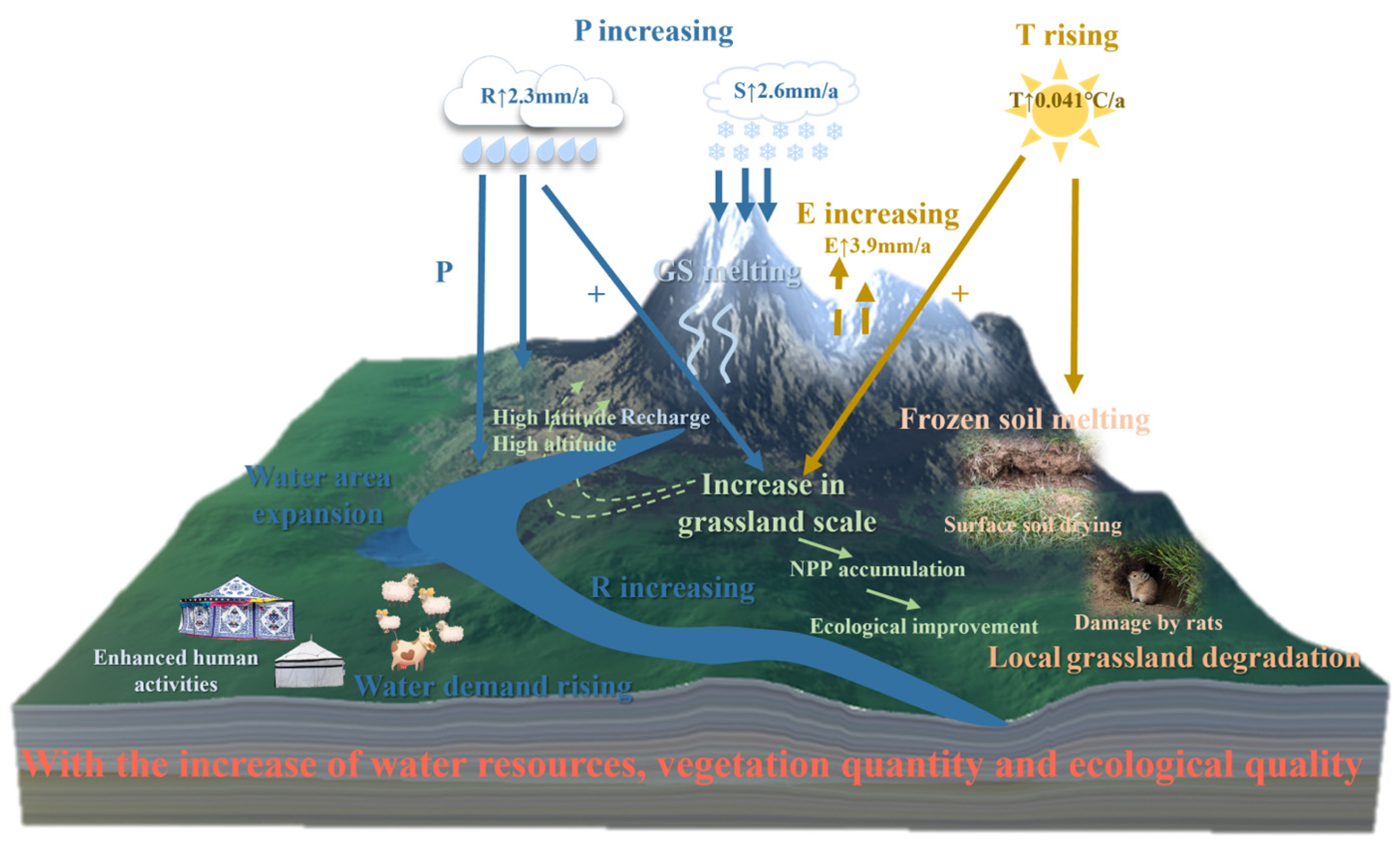
The warming–wetting trend is driving complex water–land–ecology interactions across the alpine plateau (Figure 1). Increased precipitation and rising temperatures accelerate glacier melt and permafrost degradation [4,5], leading to lake expansion and altered runoff regimes [6]. However, permafrost thaw can also trigger soil desiccation and enhance evapotranspiration, potentially inhibiting shallow-rooted vegetation growth [7]. Concurrently, the warming–wetting climate exerts positive drivers on alpine ecosystems, manifesting as expanded vegetation coverage and increased NPP [8,9]. These interconnected changes profoundly influence hydrological processes, alter water resource availability and distribution [10,11], and feedback on land use structure and ecosystem functions [12]. This intricate nexus creates severe, compound challenges, making the exploration of effective adaptive management strategies exceptionally urgent.

In response, the field of WLR allocation has developed a suite of methodological approaches. Methods ranging from early linear programming to contemporary intelligent optimization algorithms have been widely applied to address irrigation, agricultural, and economic optimization challenges [13,14,15]. The research paradigm has gradually shifted from unidirectional perspectives towards integrated WLR allocation, with recent studies incorporating multi-dimensional objectives encompassing water quantity, quality, and ecological aspects [16], as well as system risk [17] and dynamic land use–water cycle feedback [18,19,20]. However, it is evident that there are significant differences in how ecology is considered across different studies. Some studies treat ecological water demand as a constraint to ensure that water for ecological purposes is not displaced while others treat ecological benefits as a synergistic gain in the optimization objective, though they do not feature directly in the objective function; studies that treat core ecological functions directly as optimization objectives remain relatively few. Furthermore, most of these studies are based in areas of intense human activity, and their allocation objectives are often geared towards socio-economic output. By contrast, ecosystems in high-altitude cold plateaus are fragile, with complex water phases and a critical role played by solid-state water; the core objective of their management lies in maintaining and enhancing ecological functions. At present, there is a scarcity of research on the coordinated allocation of water and land resources that takes into account the specific characteristics of these regions and directly incorporates core ecological functions as optimization objectives.

In view of this, this study takes the upper reaches of the Yellow River as a case study and aims to establish a multi-objective optimization framework for the allocation of soil and water resources that is suitable for high-altitude cold plateau regions and geared towards enhancing ecological functions. Given that water conservation capacity directly reflects a catchment’s ability to regulate water supply against the backdrop of the degradation of ‘solid reservoirs’ (glaciers and permafrost) in high-altitude cold regions; vegetation water use efficiency comprehensively characterizes the adaptive growth of vegetation under climate change and serves as a key indicator for assessing ecosystem health; and soil erosion rates directly reflect the strength of a catchment’s soil and water conservation functions. These three factors, representing water regulation, vegetation health and soil conservation, respectively, collectively constitute the core characterization system of ecological functions in alpine regions. Consequently, water conservation capacity (WCC), water use efficiency (WUE) and soil erosion amount (SEA) have been selected as core ecological function indicators. The innovative aspects of this study are primarily reflected in three areas: First, we construct a WLR system network that explicitly characterizes the complex “water–land–ecology” feedbacks unique to alpine regions. Second, the model introduces an objective shift: it directly incorporates the minimization of regional water shortage, maximization of WCC, optimization of vegetation growth conditions, using WUE as a key indicator, and minimization of SEA as primary targets. This transformation elevates ecological enhancement from an implicit constraint to an explicit core objective. Finally, the study generates forward-looking allocation schemes for 2030, 2035, and 2060 under multiple climate scenarios (SSP1-2.6, SSP2-4.5, SSP3-7.0, and SSP5-8.5), providing scientific insights for decision-makers in alpine plateau regions confronting future climate change.

2. Materials and Methods

2.1. Study Area

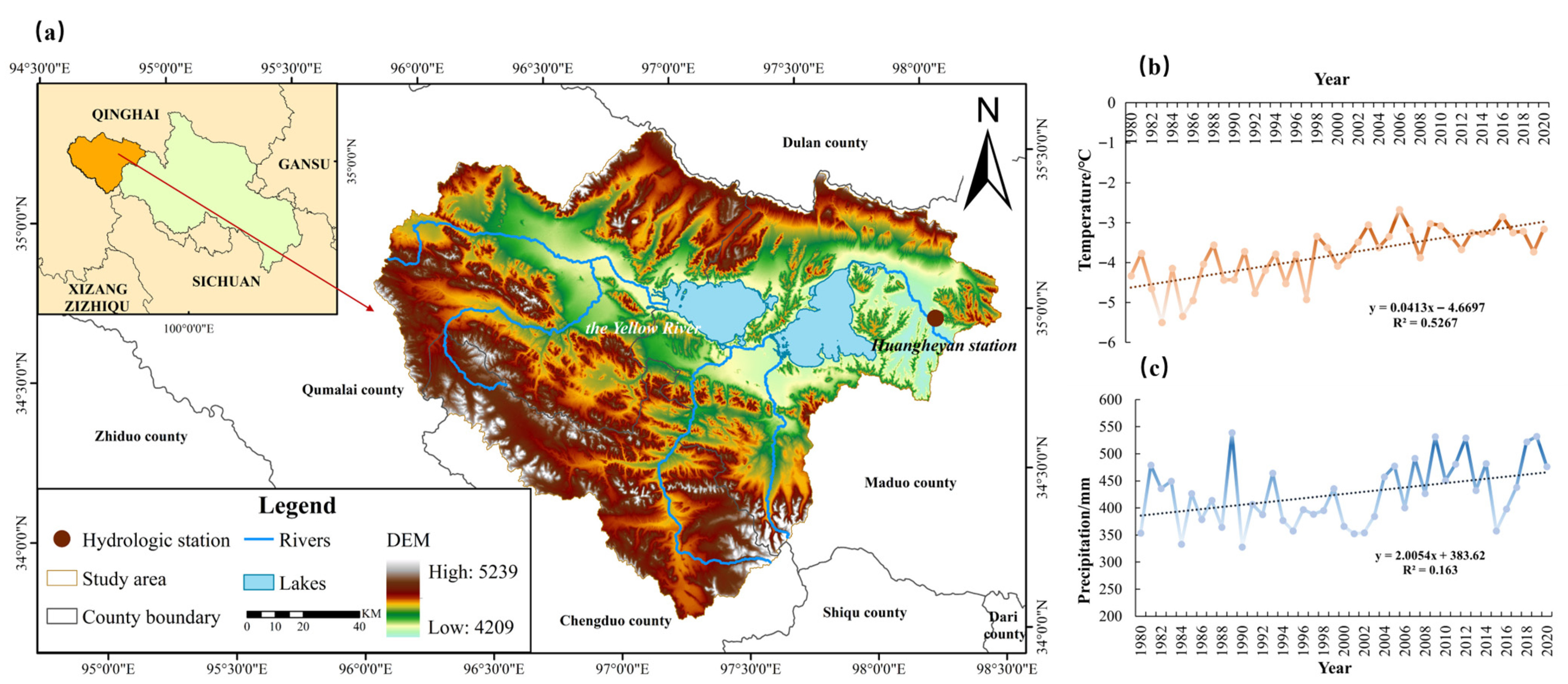
The source region of the Yellow River above the Huangheyan Station (YRSR-HHY) refers to the catchment area above the Huangheyan Hydrological Station (Figure 2a). It is located in the eastern Qinghai–Tibet Plateau and covers a total area of approximately 21,000 km². The basin is characterized by a well-developed river system, with Gyaring Lake and Ngoring Lake serving as the first and second largest freshwater lakes in the region, respectively. Land cover is dominated by alpine meadows and steppes, with grassland accounting for 83.2% of the total area in 2020. Climatically, the area experiences a typical continental plateau climate; over the long-term period of 1980–2020, the mean annual precipitation and temperature were 425.7 mm and −3.80 °C, respectively, both exhibiting increasing trends at rates of 2.01 mm/yr and 0.041 °C/yr. Specifically, the mean annual precipitation during 2000–2020 was 1.10 times that of 1980–1999, and the mean annual temperature increased by 22.06% compared to the same baseline. Overall, the region exhibits a clear “warming–wetting” trend when comparing these two periods (Figure 2b,c). The average annual runoff and total water resources from 2000 to 2020 were 819 million m³ and 3.526 billion m³, respectively. Administratively, the YRSR-HHY spans seven townships across three counties in two prefectures. Its economic structure is simple and dominated by livestock husbandry, with no significant industrial activity. In 2020, the total population was 31,045, and the gross output value of animal husbandry reached 128.59 million yuan.

2.2. Data Sources

To systematically analyze the evolution of key elements in the water–land resource system and accurately project their future trends under climate scenarios, this study employed multiple datasets from reliable sources.

Land use data were obtained from the Resource and Environment Science and Data Center (RESDC) of the Chinese Academy of Sciences (https://www.resdc.cn/ (accessed on 3 March 2024)), comprising five periods (2000, 2005, 2010, 2015, and 2020) at a spatial resolution of 30 m, making them suitable for analyzing long-term changes in land use types and patterns. Topographic data were derived from the NASADEM digital elevation model (https://www.earthdata.nasa.gov/esds/competitive-programs/measures/nasadem, (accessed on 3 March 2024)) with a spatial resolution of 30 m, used to extract watershed boundaries, river networks, and slope information. Permafrost data, consisting of vector data on seasonal and permanent permafrost distribution at two-year intervals from 2010 to 2020, were sourced from published research based on an improved TTOP model [21].

The meteorological data comprises annual precipitation and temperature observations from China Meteorological Administration stations between 2000 and 2020 (including 25 national-level meteorological stations in Qinghai Province), and 500 m resolution raster data was generated using the inverse distance weighting (IDW) method (http://data.cma.cn/ (accessed on 3 March 2024)). Water resources and water use data, covering municipal-level surface water and groundwater resources, water supply, and water consumption for domestic, ecological, and livestock uses from 2000 to 2020, were obtained from the Qinghai Water Resources Bulletin and Qinghai Statistical Yearbook (http://slt.qinghai.gov.cn/ (accessed on 3 March 2024); http://tjj.qinghai.gov.cn/ (accessed on 3 March 2024)). Vegetation data consisted of annual NPP at 500 m resolution for 2000–2020 from the MOD17A3HGF version (https://modis.gsfc.nasa.gov/ (accessed on 3 March 2024)). Socioeconomic data, including GDP and 1 km resolution population density raster data from 2000 to 2020, were also acquired from RESDC (https://www.resdc.cn/ (accessed on 3 March 2024)).

Future climate scenario data were obtained from the Coupled Model Intercomparison Project Phase 6 (CMIP6) (https://esgf-node.llnl.gov/projects/cmip6/, accessed on 5 March 2024), including monthly precipitation and temperature data for 2020–2060 under four Shared Socioeconomic Pathways (SSP1-2.6, SSP2-4.5, SSP3-7.0, and SSP5-8.5) at a spatial resolution of 0.5° × 0.5°, a bilinear interpolation method was used to downscale the data to a 500 m grid, and bias corrections were applied to precipitation and temperature data based on historical observations. This data serves as the input for future scenario analyses.

All datasets were processed using ArcGIS 10.2 software, incorporating inverse distance weighting interpolation, downscaling, and resampling techniques. The final unified datasets share a consistent Krasovsky_1940_Albers coordinate system and 500 m × 500 m spatial resolution, ensuring data quality and spatiotemporal consistency for subsequent analysis.

2.3. Technical Route

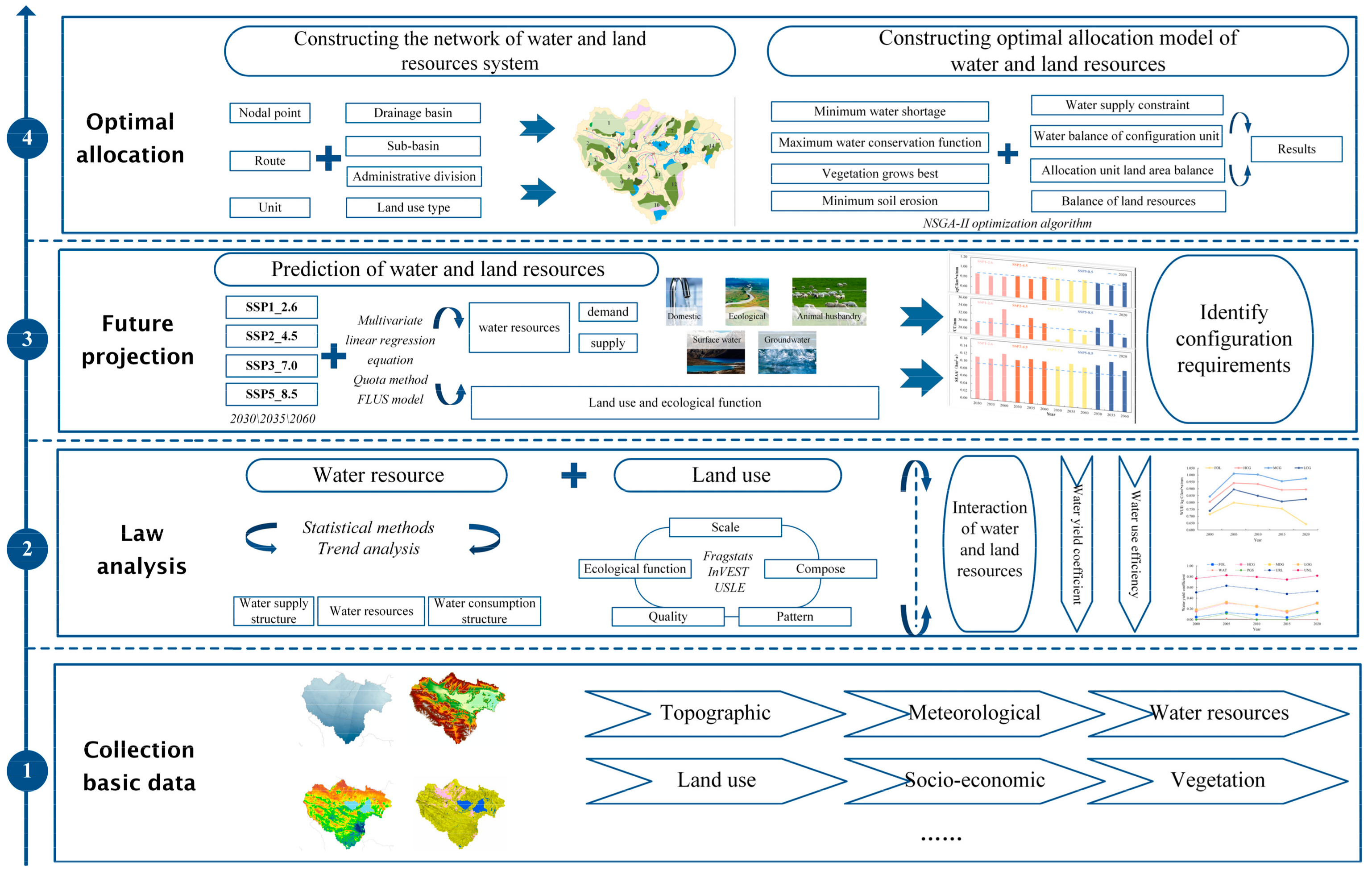
This study was conducted following a logical framework of data collection, pattern analysis, future projection, and optimal allocation, with the detailed technical roadmap presented in Figure 3.

In the data collection phase, raw datasets underwent rigorous reliability assessment and preprocessing. This included statistical analysis, gap-filling, format conversion, and spatiotemporal resolution unification to construct consistent and analyzable datasets.

For pattern analysis, multiple modeling approaches were integrated, including the Integrated Valuation of Ecosystem Services and Tradeoffs model (InVEST), the Universal Soil Loss Equation (USLE), and Fragstats 4.2, to evaluate historical changes in WLR and ecological quality. This analysis combined statistical methods and geographic information system techniques to systematically characterize spatiotemporal evolution trends.

The future projection phase incorporated climate scenario data from CMIP6. A five-dimensional perspective was adopted, encompassing scale, composition, pattern, quality, and key ecological functions. Using the Future Land-Use Simulation (FLUS) model supplemented by multiple linear regression, this study projected future WLR dynamics and identified corresponding ecological function requirements under different climate scenarios.

In the optimal allocation phase, a WLR system network was first constructed for the basin. Based on the projection results, a multi-objective optimization model was developed with the following key objectives: minimizing regional water shortage, maximizing WCC, optimizing vegetation growth conditions, and minimizing SEA. The model was solved using the NSGA-II algorithm to generate optimal WLR allocation schemes under various future scenarios. Finally, the effectiveness of these schemes was systematically evaluated.

2.4. Methods

2.4.1. Historical Assessment and Future Projections of WLR and Ecological Functions

(1)

Historical assessment

Based on prototype observations, remote sensing data, and water resource bulletins, this study comprehensively employed the InVEST model, Fragstats4.2 landscape pattern indices, Theil–Sen Median trend estimation, and Mann–Kendall significance tests to systematically analyze the spatiotemporal evolution characteristics and interactions of WLR in the study area.

Specifically, water resource evolution was primarily analyzed using statistical methods and trend analysis to assess the dynamic changes in total water resources and water supply-use structure over the past two decades. A land resource assessment was conducted from five dimensions: scale, composition, pattern, quality, and key ecological functions. The water yield and sediment retention modules of the InVEST model were utilized to assess WCC and SEA, respectively. This freely available, open-source, and widely applied model [22,23,24] operates on the principle of redistributing precipitation based on the water balance equation to calculate water conservation, while employing the USLE to quantitatively estimate soil erosion by factoring in rainfall, soil properties, topography, vegetation cover, and management practices. For details on the specific calculation process and key parameters, please refer to the Supplementary Materials.

Following established methodologies [25,26,27,28], the Fragstats 4.2 model was applied to calculate a suite of landscape pattern indices, including the Number of Patches (NP), Largest Patch Index (LPI), Edge Density (ED), Mean Patch Area (AREA_MN), Area-Weighted Mean Patch Fractal Dimension (FRAC_AM), Contagion (CONTAG), Shannon’s Diversity Index (SHDI), Shannon’s Evenness Index (SHEI), and Aggregation Index (AI), at the patch, class, and landscape levels to quantify the composition and spatial configuration of land use. Furthermore, a combination of Theil–Sen Median trend estimation and Mann–Kendall significance tests was employed to analyze the changing trends and statistical significance of key parameters, like vegetation NPP, a methodological pairing recognized for its effectiveness in identifying monotonic trends and assessing their reliability.

For analyzing water–land resource interactions, the WUE indicator was used to reveal the influence of water resource conditions on vegetation growth status, while the water yield coefficient was utilized to analyze the impact of different land cover types on the formation and transformation of water resources. WUE is defined as the ratio of NPP to potential evapotranspiration (ET), and was calculated using the following formula:

$$WU{E}_{xy}={\displaystyle \frac{NP{P}_{xy}}{P{E}_{xy}}}$$

(1)

Here, WUE_xy represents the vegetation water use efficiency for land use type x at pixel y, in kg C/km²·a/mm; NPP_xy represents the net primary productivity for land use type x at pixel y, in kg C/km²·a; and PE_xy represents the potential evapotranspiration for land use type x at pixel y, in mm.

(2)

Future projection

Guided by the near-, medium-, and long-term development objectives established in the Outline of Ecological Protection and High-Quality Development in the Yellow River Basin issued in 2021, this study set 2030, 2035, and 2060 as the near-term, medium-term, and long-term planning horizons, respectively, for the YRSR-HHY. Projections of water and land resources and ecological functions were conducted under four Shared Socioeconomic Pathway (SSP) scenarios: SSP1-2.6, SSP2-4.5, SSP3-7.0, and SSP5-8.5.

Water resources projection drew primarily on planning documents such as the Qinghai Province 14th Five-Year Plan, the National Population Development Plan (2016–2030) issued by the State Council, the Qinghai Province Water Use Quota, and the Qinghai Province Implementation Measures for the Strictest Water Resources Management Assessment. Water demand was projected for three sectors: domestic, ecological, and livestock. Domestic water demand was estimated using the quota method. First, a population projection equation was developed based on the demographic trends observed from 2000 to 2020; validation of this equation yielded a mean error of 0.05%. The projected population for each planning year was then combined with per capita domestic water quotas (derived from the Qinghai Province Water Use Quota) to obtain domestic water demand. Ecological and livestock water demands were estimated using trend extrapolation. Fitted equations were constructed based on ecological water use data from 2007 to 2020 and livestock water use data from 2000 to 2020, respectively, with mean errors of 16.51% and 0.24%, both considered acceptable. The fitting equations for domestic water demand, ecological water demand, and livestock water demand are given in Equations (2), (3), and (4), respectively.

$$W_L=N_{pop}\times Q_L\times 365\times 0.001\times {10}^{-4}$$

(2)

In the formula, W_L represents the planned annual domestic water demand for the YRSR-HHY, in 10,000 m³; N_POP represents the population of the YRSR-HHY; Q_L represents the per capita daily domestic water consumption in the Yellow River basin upstream of Yan, in L/day. The population in the YRSR-HHY is relatively small, and extreme fluctuations such as population surges or sharp declines are rare. Based on national, provincial, and municipal development plans, the population is projected to increase in the future, reaching a peak in 2030, after which it will decline. It is expected to continue declining until the middle of the 21st century, at which point the population is projected to begin a recovery trend. Therefore, the forecast for the population in the YRSR-HHY takes into account the patterns of population change within the basin from 2000 to 2020 and the natural population growth rate. By constructing mathematical equations, the population figures for the target years 2030, 2035, and 2060 are derived.

$$y=2.2656x+4.3153$$

(3)

In the equation: y represents the annual planned ecological water demand for the YRSR-HHY, in 10,000 m³; x represents the year index, where 2007 is 1, 2008 is 2, and so on. The R² value of the fitted equation is 0.57. To verify the accuracy of the fitted equation, ecological water demand for the period 2007–2020 was simulated using this equation and compared with actual values. The average error was 16.51%, with a minimum error of only 4.80%. The fitted equation can be used for subsequent predictions of ecological water demand.

$$y=162.21ln(x)+1131.2$$

(4)

In the equation, y represents the annual planned water demand for livestock farming in the YRSR-HHY, in 10,000 m³; x represents the year in the time series, where 2000 is 1, 2001 is 2, and so on. The R² value of the fitted equation is 0.78.

Available water supply was projected using multiple regression methods, drawing on historical supply–use structures and projected trends in water resources under the different climate scenarios. Water supply availability was estimated using multiple regression analysis based on historical water supply and demand patterns and trends in water resource availability under future climate scenarios. Mathematical equations (Equations (5) and (6)) were developed using the Curve Fitting Tool in MATLAB2016, based on the historical relationship between precipitation and surface water supply and groundwater supply from 2000 to 2020. All equations passed the significance test (p < 0.05), with coefficients of determination R² of 0.72 (surface water) and 0.67 (groundwater), respectively. Based on future precipitation under the four scenarios—SSP1-2.6, SSP2-4.5, SSP3-7.0, and SSP5-8.5—the available surface water and groundwater supplies for 2030, 2035, and 2060 were projected. The specific equations are as follows:

$$S{W}_S=\mathrm{25,740}\times \mathrm{SIN}(0.009587\times \mathrm{PRE}+5.069)+\mathrm{20,330}\times \mathrm{SIN}(0.01293\times \mathrm{PRE}+13.07)$$

(5)

$$S{W}_G=379.8\times \mathrm{SIN}(\mathrm{PRE}\times 0.01745-0.5202)+235\times \mathrm{SIN}(\mathrm{PRE}\times 0.03161+2.59)$$

(6)

In the equation: SW_S represents the future available surface water supply in the YRSR-HHY, SW_G represents the future available groundwater supply in the YRSR-HHY, and PRE represents precipitation under different future scenarios.

Land resources projection was carried out using an improved FLUS model based on the land use transition matrix for 2000–2020. In addition to conventional driving factors (DEM, slope, aspect, population density, GDP), the model incorporated snowfall, rainfall, temperature, and permafrost distribution data to better represent the influence of cryospheric components on land use change in this alpine region [29]. The model was configured with a random sampling mode (sampling rate = 50) and 13 hidden layers in the neural network. Validation was conducted by simulating 2020 land use using 2010 data; the resulting Kappa coefficient was 0.97, and the simulated spatial patterns closely matched the actual distributions, confirming the suitability of the improved FLUS model for future land use projection in the basin. Based on these projections, landscape pattern indices were calculated using Fragstats 4.2 to assess future landscape dynamics.

Ecological functions projection was conducted using pixel-scale multiple regression relationships between NDVI/NPP and precipitation/temperature established from historical data (2000–2020). These relationships were then applied to future climate data under the four SSP scenarios to project NDVI and NPP for 2030, 2035, and 2060. Based on these projected vegetation and climate inputs, water conservation capacity (WCC) and soil erosion amount (SEA) were calculated using the same methods as in the historical assessment to evaluate future trends in ecological functions and to identify corresponding optimization needs.

Based on the historical assessment and future projections described above, a multi-objective optimization model was developed to incorporate water conservation capacity (WCC), vegetation water use efficiency (WUE), and soil erosion amount (SEA) as core ecological function objectives. WCC optimization is achieved by adjusting the area of different land use types within each allocation unit, as different land use types exhibit significant differences in water yield and retention capacity. WUE optimization is achieved by enhancing vegetation cover and improving vegetation growth conditions, and is co-optimized with WCC and SEA in the model. SEA optimization reduces soil erosion risk by increasing vegetation cover and adjusting land use structure. These ecological function requirements are translated into concrete parameterized expressions through the objective functions (F₂, F₃, F₄) and their associated constraints in the optimization model.

2.4.2. Network Construction of WLR System

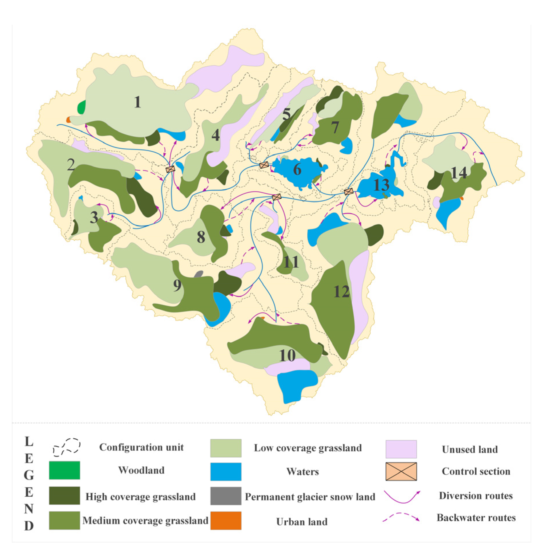
The allocation network of the WLR system in the YRSR-HHY was developed as a simplified schematic representation of key components within the basin, including WLR system, to depict upstream–downstream relationships and water supply–use connections. As shown in Figure 4, the network primarily comprises WLR users, water source and land resource nodes, basic allocation units, and allocation pathways. Taking into account the water consumption characteristics of domestic, ecological, and livestock uses, as well as the practical requirements for fine-scale management and the regulation of WLR, the study area was divided into 14 basic allocation units. This division followed a nested hierarchical framework of “watershed–sub-basin–administrative unit–land use type,” incorporating eight sub-basins, three county-level administrative regions, and eight land use types.

When disaggregating water resources and water use data to the 14 basic allocation units, the finest available data were at the county level, limited by data availability. Since not every allocation unit contains all land use types (e.g., urban land, forest land), a simple area-weighted averaging approach would be inappropriate. Therefore, we adopted a “land use–water use association method” for spatial downscaling. The procedure is as follows:

(1)

Domestic Water Use Allocation: Domestic water use was associated with urban land (URL). First, the average domestic water use per unit area of urban land was calculated by dividing the total county-level domestic water use by the total area of urban land within that county. Then, for each basic allocation unit, the domestic water use was calculated by multiplying the area of urban land in that unit by the per-unit-area domestic water use coefficient.

(2)

Ecological Water Use Allocation: Ecological water use was associated with forest land (FOL) and grassland (HCG, MCG, LCG). Because ecological water use is primarily for maintaining natural vegetation, it was allocated to each unit in proportion to the area of forest and grassland within the unit.

(3)

Livestock Water Use Allocation: Livestock water use was also associated with urban land (URL). Livestock husbandry is the dominant industry in the basin, and livestock activities are concentrated around urban land areas. Therefore, livestock water use was allocated using the same method as domestic water use, based on the area of urban land in each unit.

Using this method, county-level statistical data were reasonably disaggregated to the 14 basic allocation units, yielding a water resources supply–demand dataset consistent with the spatial distribution of land use. While not perfect, this approach provides a scientifically sound representation of spatial variations in water resources and water use under the available data constraints.

2.4.3. Construction of Optimal Allocation Model of WLR

Based on the aforementioned WLR system allocation network for the YRSR-HHY, an optimal allocation model for WLR was developed using Python v2021.2.4 programming. The overall objectives were defined according to future requirements for WLR and ecological function enhancement, including minimizing regional water shortage, maximizing water conservation capacity (WCC), optimizing vegetation growth conditions, and minimizing soil erosion amount (SEA). Constraints were established based on projected WLR under future climate scenarios, including water supply constraints, water balance constraints for each allocation unit, land area balance constraints per allocation unit, and overall land resource balance constraints.

The optimal allocation of WLR in the YRSR-HHY is a multi-objective joint regulation problem. The overall goal is:

$$F=\left\{\begin{array}{l}Min{F}_1\\ Max{F}_2\\ Max{F}_3\\ Min{F}_4\end{array}\right.$$

(7)

In the formulation, Min F₁ represents the objective of minimizing water shortage in the basin; Max F₂ denotes the objective of maximizing WCC; Max F₃ corresponds to the objective of optimizing vegetation growth conditions, which is quantitatively assessed using vegetation WUE as a key ecological indicator; and Min F₄ indicates the objective of minimizing SEA. The specific definitions and mathematical expressions of each objective function are provided in

Table 1. Expression and meaning of objective function and constraint conditions.

Objective Functions	Meaning
$F_1={\displaystyle \sum _{n=1}^N{\displaystyle \sum _{y=1}^Y\left[{\displaystyle \sum _{x=1}^X(W{R}_{nxy}\times L_{nx})-W{S}_{ny}}\right]}}$	Water Shortage Minimization Objective: This objective is characterized by the degree to which the allocated water supply meets the total water demand across the basin. A lower water shortage rate indicates better fulfillment of user demands, whereas a higher rate reflects unmet needs and potential water scarcity risks, which may adversely affect domestic and ecological development in the region.
$F_2={\displaystyle \sum _{n=1}^N\frac{{\displaystyle \sum _{x=1}^X{W}_{nx}\times L_{nx}}}{{\displaystyle \sum _{x=1}^X{L}_{nx}}}}$	WCC Maximization Objective: This objective is quantified by the total WCC across the basin. A higher value indicates stronger water retention functionality within the watershed, while a lower value reflects weaker capacity.
$F_3={\displaystyle \sum _{n=1}^N\frac{{\displaystyle \sum _{x=1}^{X}WU{E}_{nx}\times L_{nx}}}{{\displaystyle \sum _{x=1}^X{L}_{nx}}}}$	Vegetation Growth Condition Optimization Objective: This objective aims to improve the overall vitality and health of the ecosystem by optimizing WLR allocation. Vegetation WUE at the watershed scale is employed as a comprehensive indicator to evaluate the achievement of this objective. Higher WUE values signify more efficient water utilization by vegetation, indicating improved vegetation growth vigor, resilience, and overall ecological quality under the allocated scheme.
$F_4={\displaystyle \sum _{n=1}^N\frac{{\displaystyle \sum _{x=1}^{X}S{E}_{nx}\times L_{nx}}}{{\displaystyle \sum _{x=1}^X{L}_{nx}}}}$	SEA Minimization Objective: This objective is measured by the SEA per unit area across the basin. Lower values demonstrate more stable land quality and enhanced ecological environment sustainability within the watershed.
Constraint Conditions	Meaning
${\displaystyle \sum _{n=1}^N{\displaystyle \sum _{y=1}^{Y}W{S}_{ny}}}\le {\displaystyle \sum _{y=1}^Y{W}_y}$	Water supply constraint means that the available water supply of a certain water source in the basin is not higher than the water supply capacity of the water source in the basin.
${\displaystyle \sum _{y=1}^Y{\displaystyle \sum _{x=1}^X\left(W{R}_{nxy}\times L_{nx}\right)}}=WA{S}_n$	The water balance constraint of the configuration unit means that the actual water supply of each basic configuration unit after configuration is equal to the water demand of each type of land use in the basic configuration unit.
$\begin{array}{l}{\displaystyle \sum _{x=1}^X{L}_{nx}}=L_n\\ L_{nx\_d}\le L_{nx}\le L_{nx\_u}\end{array}$	The land area balance constraint of configuration unit is when the total area of each type of land use in a basic configuration unit after configuration is equal to the area of the basic configuration unit.
$\begin{array}{l}{\displaystyle \sum _{n=1}^N{\displaystyle \sum _{x=1}^X{L}_{nx}}}={\displaystyle \sum _{n=1}^N{L}_n}\\ L_{nx\_d}\le L_{nx}\le L_{nx\_u}\end{array}$	The land resource balance constraint means that the area of all kinds of land use after allocation is equal to the total area of the basin.

In the formula, F₁ is the water shortage in the HHY, m³; N, X and Y are the total number of basic allocation units, the total number of land use types and the total number of water supply sources in the basin, respectively. The values of N, X and Y in this paper are 14, 8 and 2, respectively. n, x, and y represent the nth configuration unit in the basin (n = 1, 2, 3…14). Land use type is represented by x. (In this paper, x = 1, 2, 3…8, in which 1 is forest land (FOL), 2, 3 and 4 are high-coverage grassland (HCG), medium-coverage grassland (MCG) and low-coverage grassland (LCG), 5 is water area (WAT), 6 is permanent glacier snow (PGS), 7 is urban land (URL), and 8 is unused land (UNL).) The yth water source is represented as y = 1, 2 in this paper, where 1 is surface water and 2 is groundwater. WRnxy represents the water demand of the x-type land use per unit area in the nth configuration unit in the basin for the y-type water source, m; Lnx represents the area of type x land use in the nth configuration unit in the basin, m²; WSny denotes the amount of water available from the y-type water source to the n-configuration unit of the basin, m³; F₂ is the WCC in the HHY, mm; Wnx represents the water conservation amount of land use type x in the nth configuration unit of the basin, mm; F₃ is the WUE of vegetation in the HHY, kgC/km²·a/mm; WUEnx represents the vegetation WUE of type x land use in the nth configuration unit of the basin, mm; F₄ is the SEA in the HHY, t/(hm²·a); SEnx represents the SEA of land use type x in the nth configuration unit of the basin, t/(hm²· a); Wy is the total amount of water resources of the y-type water source, m³; WASn is the actual water supply of the nth basic configuration unit, m³; Ln is the total area of the nth basic configuration unit, m²; L_{nx_d} and L_{nx_u} represent the lower boundary and upper boundary of the constraint of the area of the x land use type in the nth configuration unit, m².

.

The multi-objective optimization model was solved using the Non-dominated Sorting Genetic Algorithm II (NSGA-II). After multiple trial runs to balance computational efficiency and solution quality, the algorithm parameters were set as follows: population size of 200, maximum number of generations (iterations) of 500, crossover probability of 0.8, and mutation probability of 0.1. These settings ensured that the Pareto-optimal front achieved stable convergence across all scenarios.

To verify the convergence and robustness of the NSGA-II algorithm, we conducted the following tests: (1) Convergence Diagnosis: We recorded changes in the Pareto front at each iteration. By approximately the 300th iteration, the front stabilized, with subsequent iterations resulting in only minor adjustments to the density of the front; (2) Multiple Independent Runs: Five independent runs were performed under the same parameter settings. The resulting Pareto fronts were essentially consistent, and the optimal solutions selected were identical, indicating that the algorithm exhibits good robustness.

It is worth noting that certain land use types, such as FOL, PGS, and URL, occupy extremely small proportions of the total basin area (<0.1%). Nevertheless, these types are retained in the model because they play indispensable roles in maintaining regional biodiversity, water source regulation (especially for glaciers as solid reservoirs), and landscape integrity. Their area adjustments are strictly constrained by lower and upper bounds derived from historical trends and ecological protection redlines, ensuring that the optimized allocation remains practically feasible and aligned with regional conservation goals. Additionally, PGS is retained as a distinct land use category, with changes in its extent driven by future climate scenarios; permafrost distribution data is used as one of the driving factors in the FLUS model to simulate the impact of permafrost degradation on land use changes; and glacial meltwater, as a key component of surface water resources, is incorporated into water supply calculations.

3. Results

3.1. Temporal and Spatial Evolution Characteristics of Historical WLR and Ecological Functions

3.1.1. Water Resource

(1)

Water Resources’ Quantity

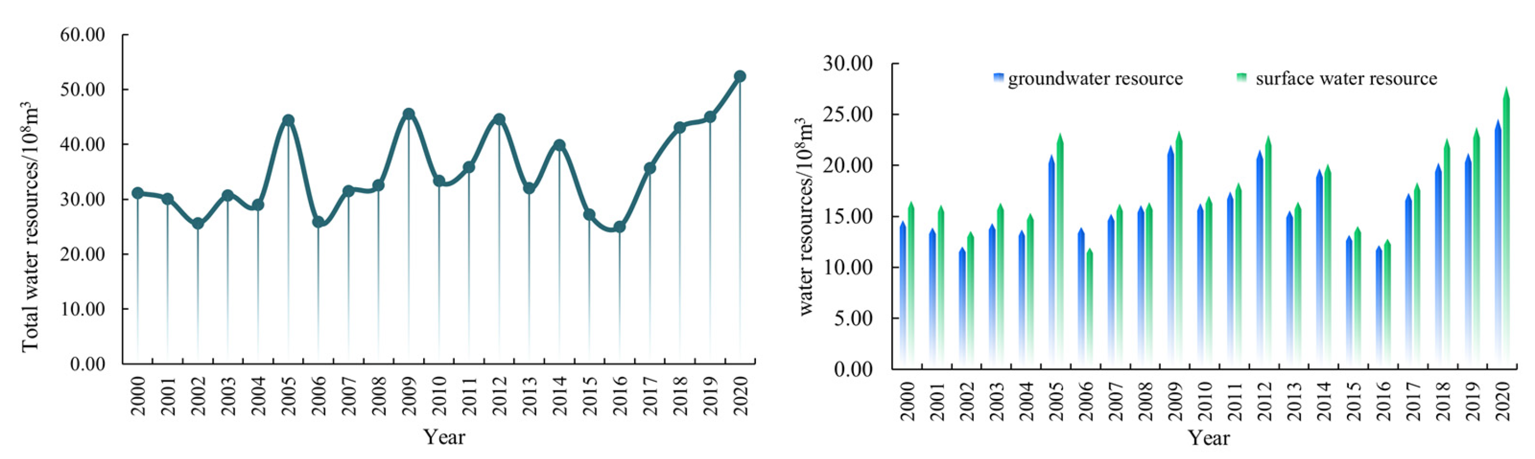
During the 2000–2020 period, the multi-year average water resources’ volume in the YRSR-HHY was 3.526 billion m³, showing an overall increasing trend at a rate of 0.063 billion m³ per year. In terms of water source composition, the resources primarily consisted of surface water and groundwater (with no double-counting). The multi-year average surface water resources amounted to 1.828 billion m³, while groundwater resources averaged 1.698 billion m³. Both components exhibited growth, with surface water increasing by 0.054 billion m³ per year and groundwater by 0.030 billion m³ per year. Notably, this upward trend persisted over the recent five-year period (Figure 5).

(2)

Water Supply and Use Structure

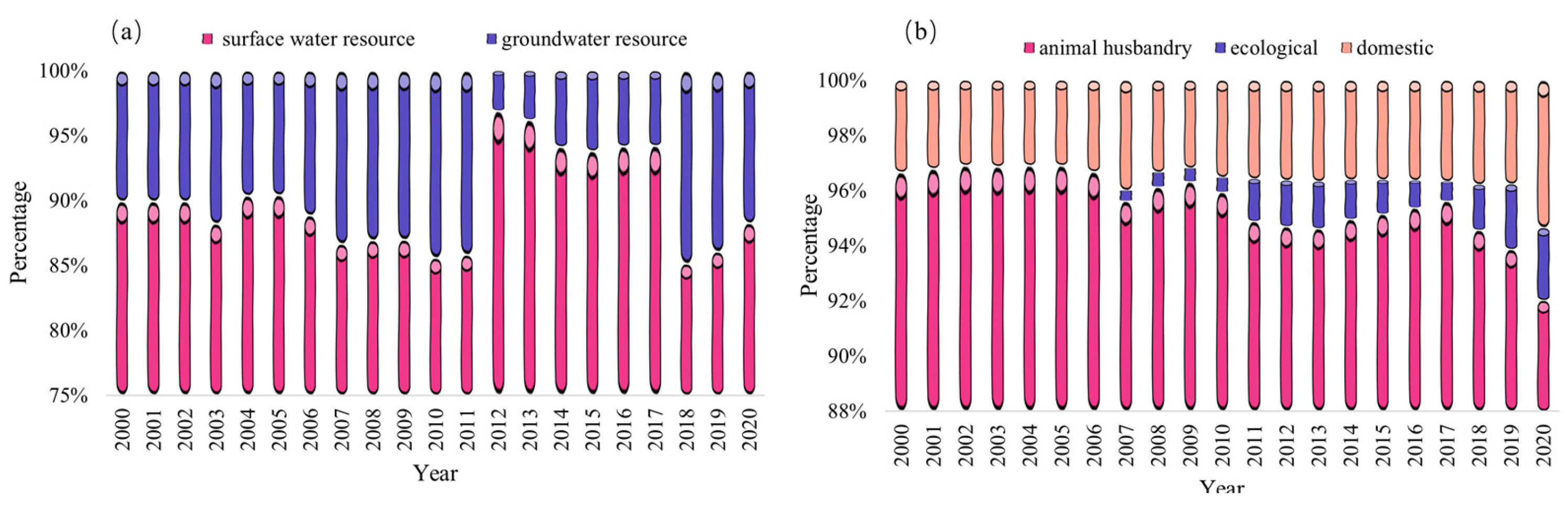
The water supply and use structure in the YRSR-HHY from 2000 to 2020 is illustrated in Figure 6. The multi-year average water supply was 15.5133 million m³, increasing at an average annual rate of 0.2428 million m³. Surface water served as the dominant supply source, accounting for 13.9593 million m³ (90.0%) of the total supply, while groundwater constituted the remainder.

Water use was primarily distributed across the domestic, livestock, and ecological sectors. Livestock husbandry represented the largest water-consuming sector, with an average annual consumption of 14.8177 million m³ (95.5% of total use). Domestic water use followed, accounting for 3.6% of the total, while ecological water use, though representing the smallest proportion, demonstrated a gradually increasing trend over the study period.

3.1.2. Land Use

(1)

Land Use Composition, Scale, and Pattern

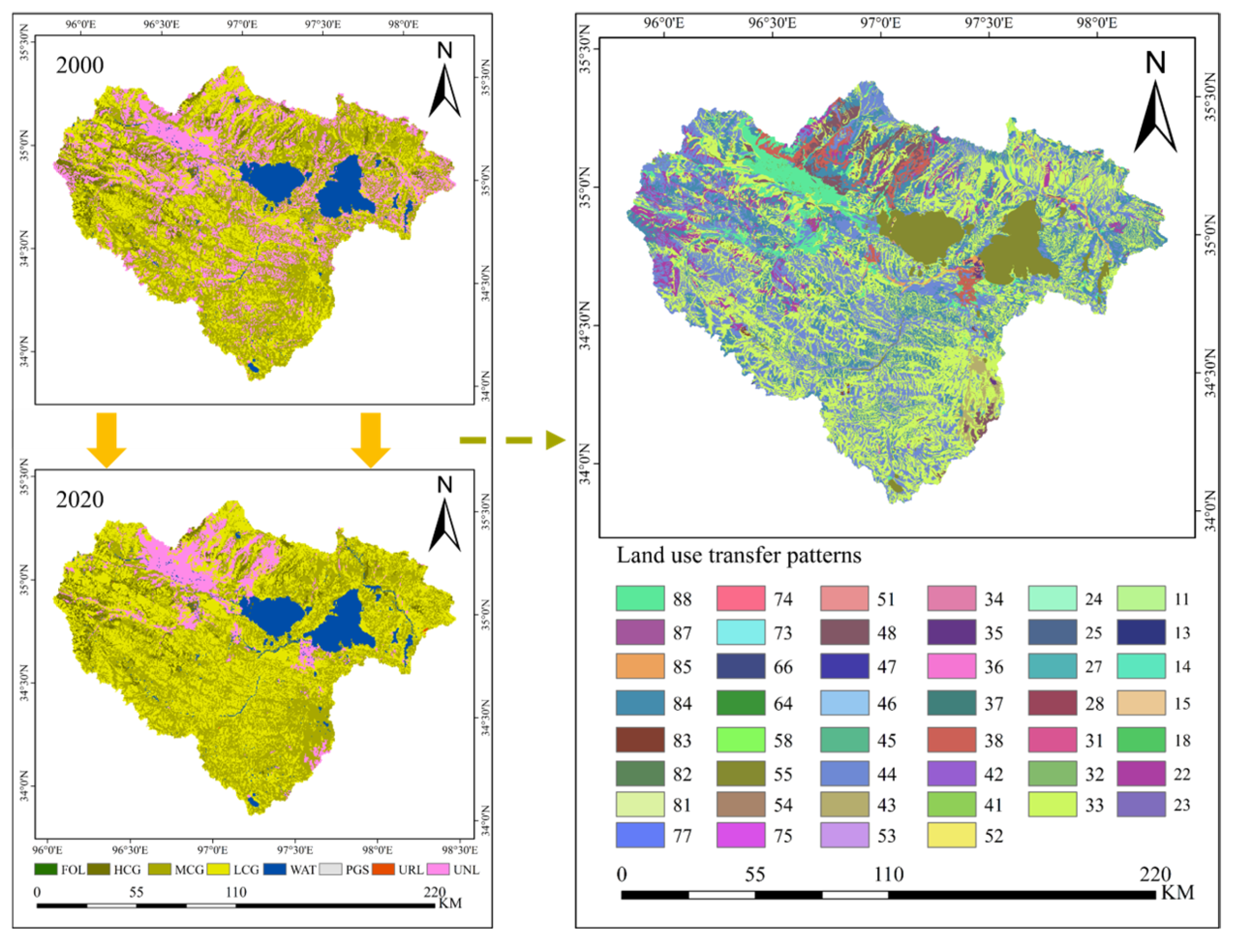
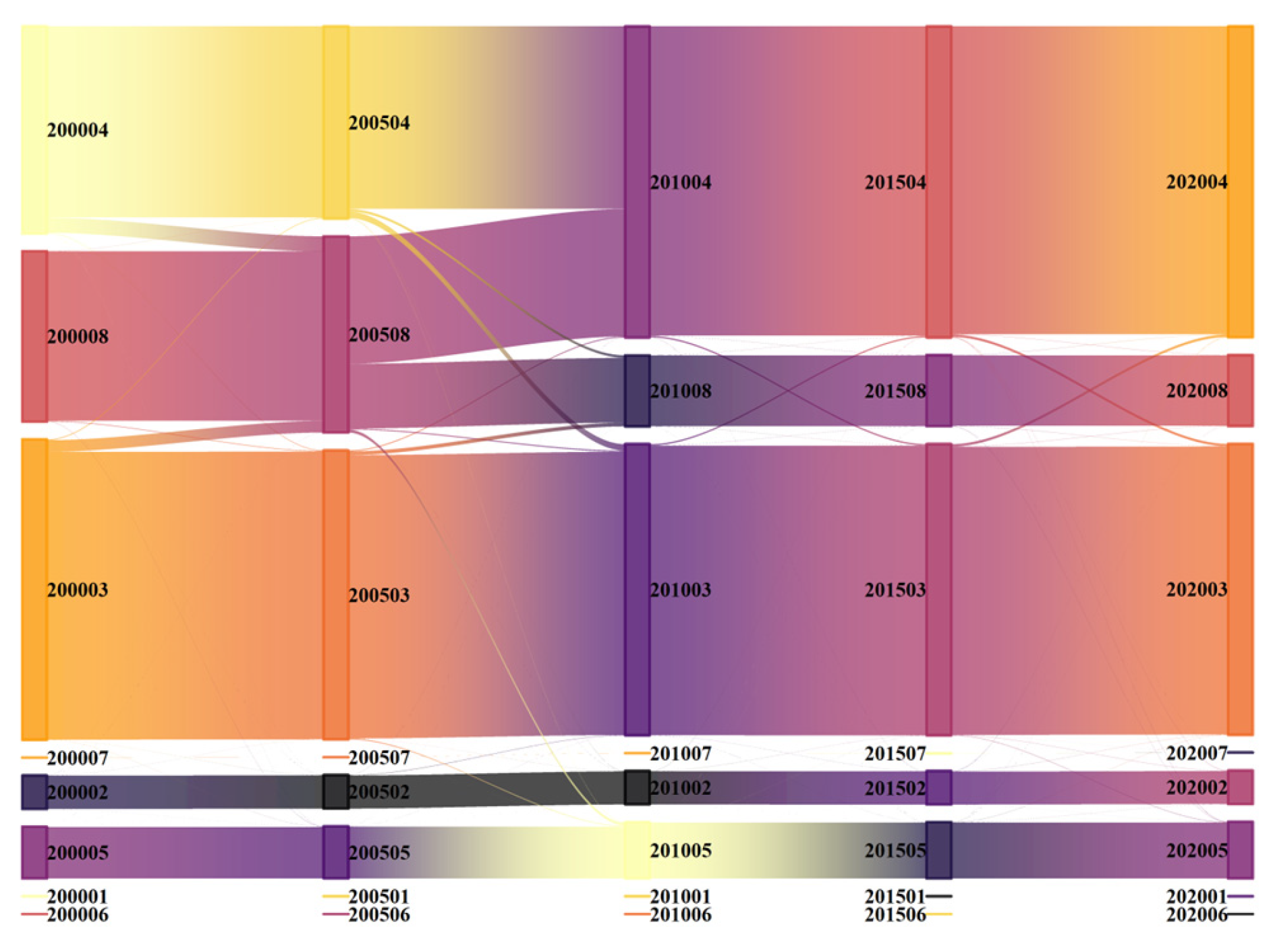
Land use in the basin comprises eight categories: FOL, HCG, MCG, LCG, WAT, PGS, URL, and UNL (Figure 7). Grassland represents the predominant land use type, primarily consisting of MCG (49.8%) and LCG (44.5%). UNL ranked second in area extent but has undergone a rapid reduction since 2005, currently accounting for less than 10.0% of the total basin area. WAT constitutes the third-largest category, with its multi-year average area representing 7.2% of the total. The remaining three categories (FOL, PGS, and URL) each occupy less than 0.1% of the total area. Over the past two decades, 4930.24 km² of land underwent a type conversion, dominated by transitions from UNL to LCG, which accounted for 3456.80 km² of the total changed area. Spatially, notable changes included the disappearance of UNL in the southern basin, the expansion of MCG in the southeastern region, and the southwestward expansion of Gyaring Lake (Figure 8). Landscape pattern analysis (

Table 2. Landscape pattern index of the study area from 2000 to 2020.

Year	NP	LPI	ED	AREA_MN	FRAC_AM	CONTAG	SHDI	SHEI	AI
2000	8286.00	18.88	26.19	252.54	1.23	62.01	1.38	0.66	96.07
2005	8183.00	18.85	25.65	255.72	1.23	61.86	1.39	0.67	96.15
2010	7114.00	19.06	24.06	294.15	1.24	64.74	1.29	0.62	96.39
2015	7100.00	19.12	23.95	294.73	1.24	64.75	1.29	0.62	96.41
2020	7096.00	19.10	24.11	294.90	1.24	64.70	1.29	0.62	96.38

) revealed decreased landscape fragmentation, as evidenced by reductions in NP (−14.4%) and ED (−7.95%). The SHDI decreased by 6.5%, while the SHEI also decreased by 6.5%, indicating an increased dominance of the dominant patch type (grassland) and greater unevenness in the distribution of patch types. The connectivity of dominant patches improved (CONTAG + 3.2%), accompanied by increased mean patch area (AREA_MN + 16.8%) and greater patch shape complexity (Area-Weighted Mean Patch Fractal Dimension [FRAC_AM] + 1.13%). The increase in Largest Patch Index (LPI + 1.15%) suggests enhanced connectivity of the dominant patch type (primarily grassland), which may be associated with vegetation recovery driven by ecological protection policies and climate change.

(2)

Vegetation Quality and Key Ecological Functions

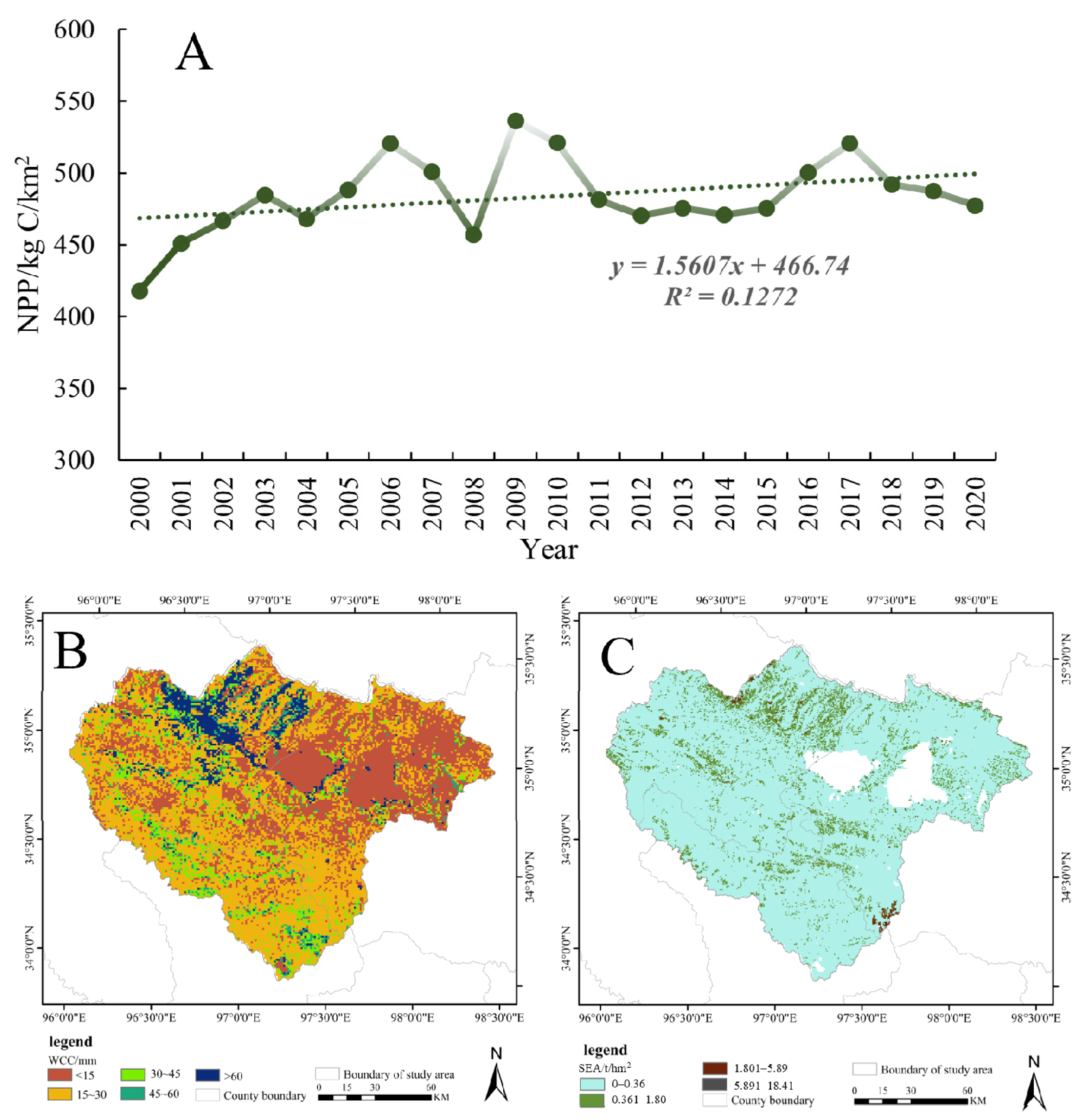
Vegetation quality demonstrated a significant improvement from 2000 to 2020. An analysis of NPP spatiotemporal patterns (Figure 9) showed a multi-year average NPP of 484.90 kg C/km², increasing at a rate of 1.56 kg C/km² per year. Spatially, NPP exhibited a “east–high–west–low, south–high–north–low” pattern. The entire basin displayed an increasing NPP trend, with 17.0% of the area showing slightly significant increase, 12.5% a significant increase, and 0.7% a highly significant increase, particularly concentrated near the basin outlet.

Key ecological functions showed a consistent improvement during 2000–2020. The multi-year average WCC was 24.5 mm, increasing at 0.1274 mm per five-year interval. Spatially, WCC displayed a “low-southeast–high-periphery” pattern. The multi-year average SEA was 0.14 t/hm², classified as slight erosion, which decreased at 0.036 t/hm² per five years, representing a 34.1% total reduction. Spatially, SEA was more severe in the southeastern and central–western regions compared to other areas.

3.1.3. Interaction of WLR

(1)

Impact of Water Resources on Land Resources

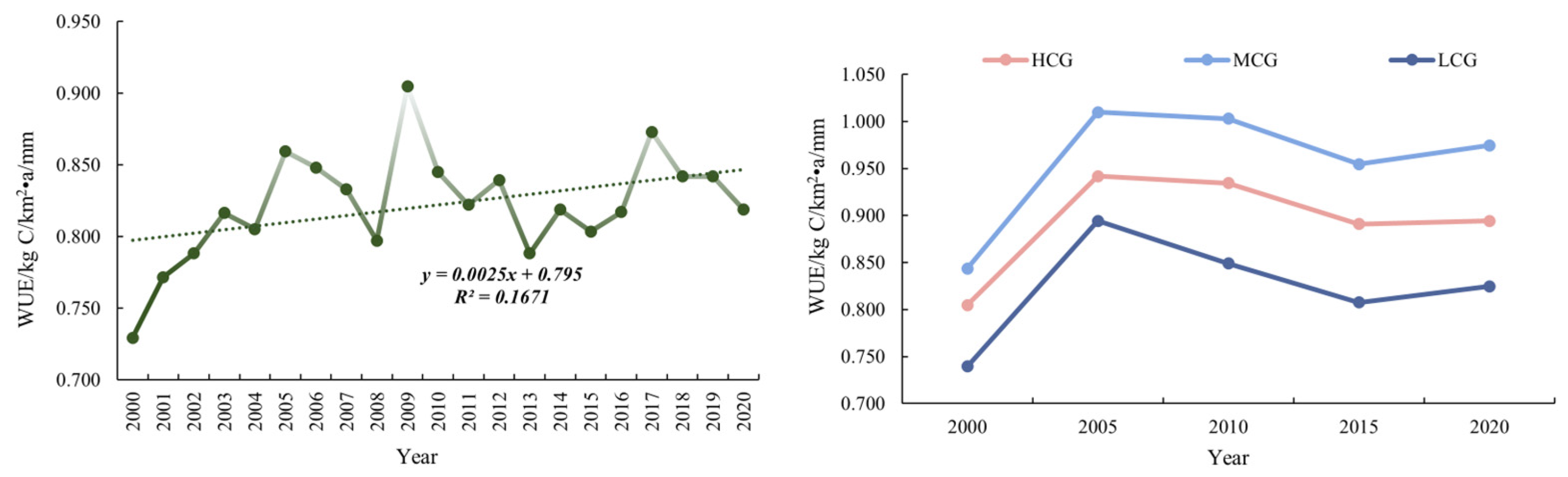
Changes in water resources within the basin alter soil moisture, structure, and nutrient conditions, thereby influencing vegetation growth status and subsequently driving changes in land use types. WUE serves as an effective indicator for characterizing WLR utilization efficiency and reflecting vegetation adaptability. During 2000–2020, the average WUE in the YRSR-HHY was 0.822 kg C·km⁻²·a⁻¹·mm⁻¹, showing an increasing trend at a rate of 0.0025 kg C·km⁻²·a⁻¹·mm⁻¹ per year. Analysis by land use type (excluding FOL due to its minimal coverage < 0.1%) revealed multi-year average WUE values of 0.893, 0.957, and 0.823 for HCG, MCG, and LCG respectively. These three grassland types exhibited WUE increases of 11.1%, 15.5%, and 11.5% over the study period. The enhancement in WUE is associated with improved vegetation growth conditions, which may contribute to vegetation expansion in the basin (Figure 10).

(2)

Impact of Land Resources on Water Resources

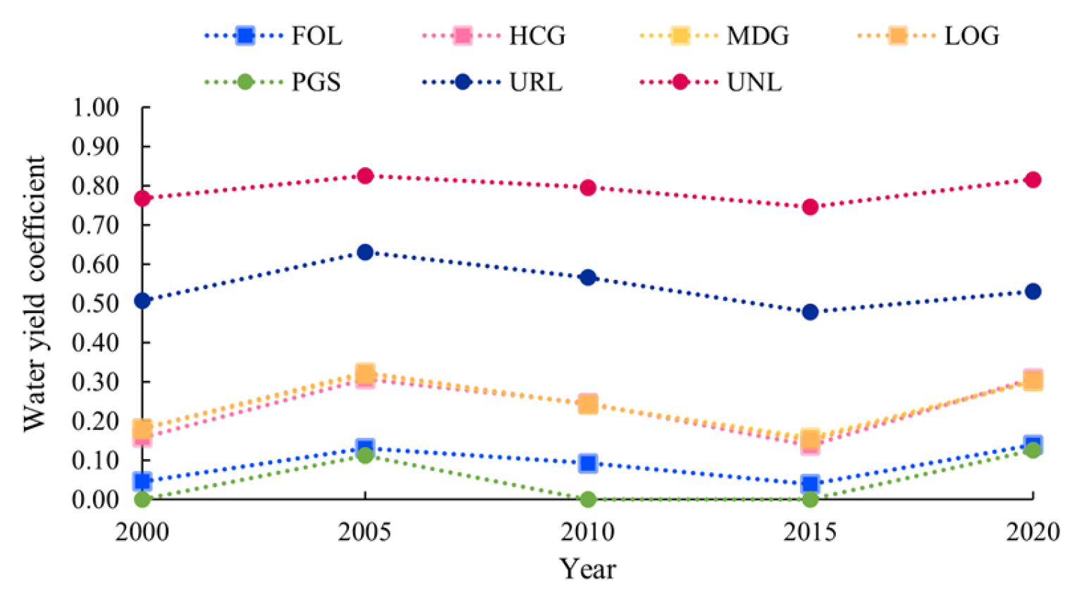
The water yield coefficient serves as an indicator of regional water production capacity. Over the past two decades, the multi-year average water yield coefficient in the basin was 0.306, showing a decreasing trend of 0.02 per five-year period. The water yield coefficients for all land use types followed an increase–decrease–increase fluctuation pattern. Among different land cover types, UNL demonstrated the highest multi-year average coefficient (0.790), at 2.58 times the basin average. URL followed with 0.542, 1.78 times the basin average. Grassland coefficients decreased with increasing coverage density, showing values of 0.2404, 0.2401, and 0.231 for LCG, MCG, and HCG, respectively. FOL and PGS exhibited the lowest coefficients at 0.089 and 0.048. These findings demonstrate significant disparities in water yield capacity across land cover types, identifying them as key drivers of variations in basin water yield and crucial factors influencing water resource abundance and allocation efficiency (Figure 11).

3.2. Future Estimation Results of WLR and Ecological Function Requirements

3.2.1. Water Resource

(1)

Available Water Supply

The projected surface water and groundwater availability under the four climate scenarios for the YRSR-HHY are summarized in

Table 3. Forecast results of available water supply in 2030, 2035 and 2060 (10⁴ m³).

Scenarios	Year	Surface Water	Underground Water Supply	Sum
SSP1-2.6	2030	1570.41	380.37	1950.79
	2035	1845.52	237.09	2082.61
	2060	2358.75	100.94	2459.70
SSP2-4.5	2030	1588.49	361.75	1950.24
	2035	1543.30	382.68	1925.98
	2060	2009.72	177.70	2187.42
SSP3-7.0	2030	1787.84	255.36	2043.20
	2035	1944.43	315.32	2259.75
	2060	1895.17	263.74	2158.92
SSP5-8.5	2030	2068.34	379.42	2447.76
	2035	1936.19	290.78	2226.97
	2060	2067.45	250.50	2317.95

. Under the enhanced warming–wetting trend, the total available water supply across the basin is expected to increase compared to the 2020 baseline. Specifically, by 2030, the available water supply under all scenarios is projected to increase by 10.2–38.3% relative to 2020. By 2035, the increase ranges between 8.8% and 27.7%, and by 2060, a 22.0–39.0% rise is anticipated. Notably, the SSP5-8.5 scenario exhibits particularly abundant water availability. In terms of supply structure, the future composition remains largely consistent with the current pattern, with surface water continuing to serve as the primary source, accounting for no less than 80% of the total supply.

(2)

Water Demand

The total water demand in the YRSR-HHY is projected to reach 18.5166 million m³, 18.9221 million m³, and 20.0723 million m³ in 2030, 2035, and 2060, respectively. Compared to the total water use in the baseline year 2020 (17.7020 million m³), these values represent increases of 4.60%, 6.89%, and 13.39% for the three target years (

Table 4. Forecast results of water demand in 2030, 2035 and 2060 (10⁴ m³).

Year	Domestic	Animal Husbandry	Ecological	SUM
2030	104.74	1688.23	58.69	1851.66
2035	109.71	1712.48	70.02	1892.21
2060	82.54	1798.02	126.66	2007.23

).

3.2.2. Land Use

(1)

Land Use Composition, Scale, and Pattern

A FLUS model was developed using the estimation method described in Section 2.4.1, achieving a Kappa coefficient of 0.97. Under the four climate scenarios for 2030, 2035, and 2060, the land use composition remains consistent with the baseline year. In terms of scale changes, the area of HCG is projected to increase by 0.77%, 1.15%, and 1.69% in 2030, 2035, and 2060, respectively, compared to the baseline. In contrast, the area of LCG is expected to decrease by 0.37%, 0.51%, and 0.73% over the same periods. WAT exhibit the most significant expansion, with a maximum increase of 3.16%, while PGS is projected to decrease by 21.68%. The utilization of UNL shows a reduction of 0.57%. Spatially, the distribution pattern shows no major differences compared to the current pattern, with primary changes concentrated in the expansion of HCG in the northwestern part of the basin and the evolution of WAT morphology in the northeast.

An analysis of landscape patterns indicates that five landscape indices, NP, LPI, ED, CONTAG, and AI, show decreasing trends in 2030, 2035, and 2060 under all scenarios compared to 2020. In contrast, four indices, AREA_MN, FRAC_AM, SHDI, and SHEI, demonstrate increasing trends. These results suggest a continued reduction in landscape fragmentation, an increasing proportion of the dominant patch type (grassland), more complex patch shapes, enhanced patch diversity, and a more balanced distribution of patch types across the landscape (

Table 5. Landscape pattern index of the study area in 2030, 2035 and 2060.

SSP1_2.6
Year	NP	LPI	ED	AREA_MN	FRAC_AM	CONTAG	SHDI	SHEI	AI
2030	2978.00	22.39	14.215	702.653	1.245	47.319	1.290	0.620	64.291
2035	2972.00	22.39	14.197	704.071	1.244	47.276	1.292	0.621	64.337
2060	2950.00	22.39	14.215	709.322	1.248	47.219	1.293	0.622	64.292
SSP2_4.5
Year	NP	LPI	ED	AREA_MN	FRAC_AM	CONTAG	SHDI	SHEI	AI
2030	2974.00	22.39	14.237	703.598	1.248	47.301	1.290	0.620	64.235
2035	2978.00	22.39	14.158	702.653	1.244	47.290	1.292	0.621	64.434
2060	2962.00	22.39	14.236	706.448	1.249	47.166	1.293	0.622	64.239
SSP3_7.0
Year	NP	LPI	ED	AREA_MN	FRAC_AM	CONTAG	SHDI	SHEI	AI
2030	2947.00	22.39	14.201	710.044	1.248	47.329	1.290	0.620	64.325
2035	2918.00	22.39	14.136	717.101	1.248	47.296	1.293	0.622	64.493
2060	2952.00	22.39	14.230	708.842	1.249	47.227	1.292	0.622	64.253
SSP5_8.5
Year	NP	LPI	ED	AREA_MN	FRAC_AM	CONTAG	SHDI	SHEI	AI
2030	2956.00	22.39	14.192	707.882	1.245	47.348	1.290	0.620	64.350
2035	2982.00	22.39	14.167	701.710	1.243	47.295	1.292	0.621	64.412
2060	2943.00	22.39	14.203	711.009	1.250	47.236	1.292	0.622	64.321

).

(2)

Vegetation Quality

NPP in the YRSR-HHY is projected to increase under all four scenarios for 2030, 2035, and 2060. The results indicate that future NPP will rise by 9.6% to 13.4% compared to 2020, with the smallest increase under the SSP1-2.6 scenario and the largest under SSP5-8.5. Across the planning years, the average NPP values for 2030, 2035, and 2060 under the four scenarios are 516.56 kg C/km², 518.59 kg C/km², and 565.70 kg C/km², respectively, representing increases of 8.2%, 8.7%, and 18.5% compared to the baseline value of 477.32 kg C/km².

From a scenario perspective, NPP in 2030 ranges from 515.41 to 517.79 kg C/km², reflecting an increase of 8.0% to 8.4% relative to 2020. In 2035, NPP ranges from 508.93 to 525.54 kg C/km², corresponding to an increase of 6.6% to 10.1%. By 2060, NPP is projected to reach 542.96 to 591.08 kg C/km², representing an increase of 13.8% to 23.8% compared to the baseline.

3.2.3. Future Ecological Function Development Requirements

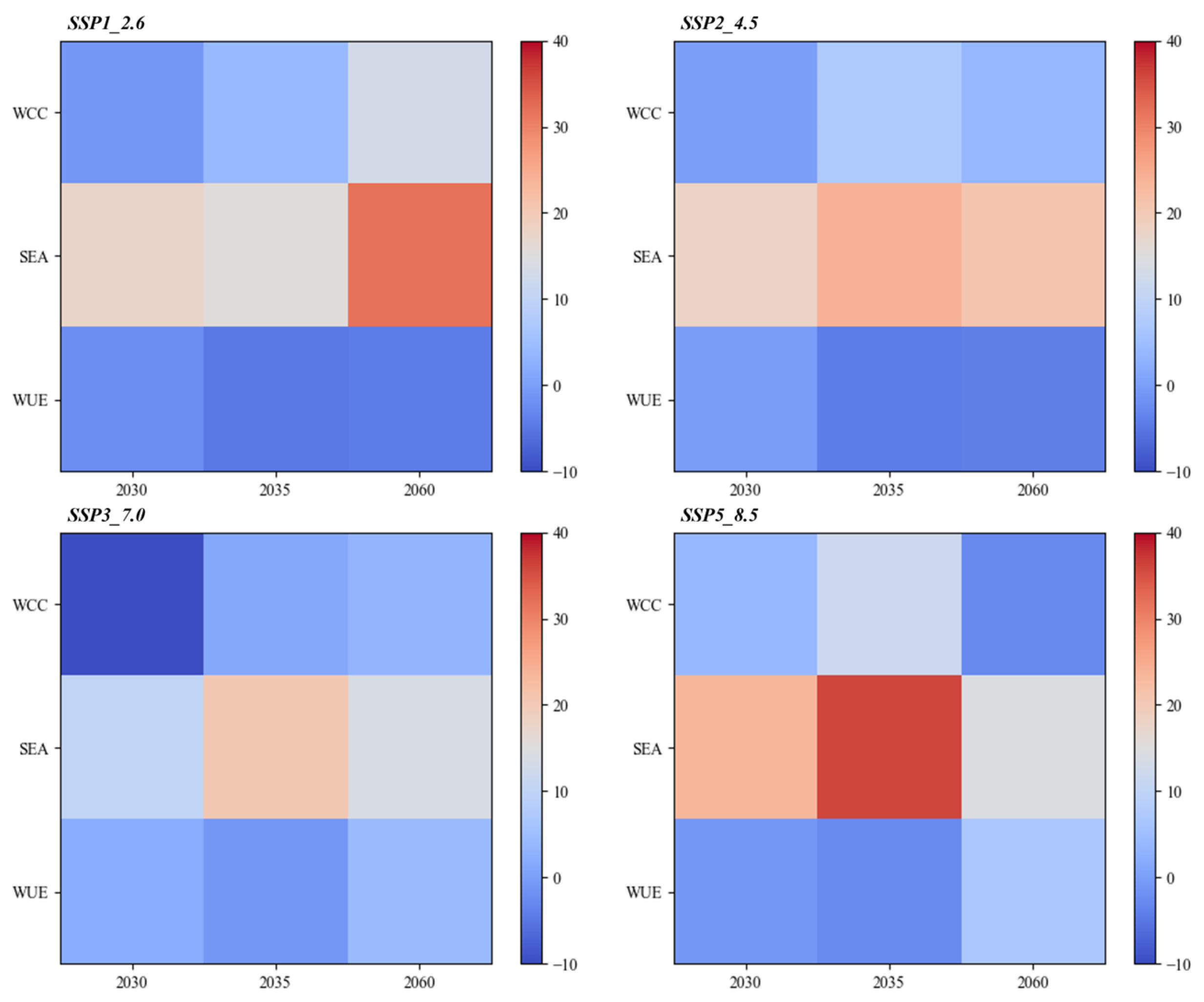
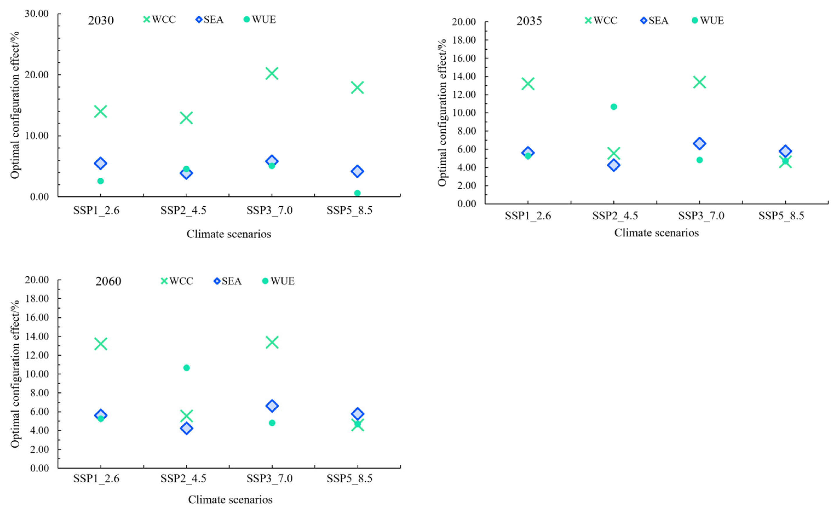
Based on the future projection data, the WCC, WUE, and SEA under the four scenarios for 2030, 2035, and 2060 were calculated and compared with the baseline year, as shown in Figure 12. The average WCC values for these years were 29.41 mm, 31.75 mm, and 30.68 mm, respectively, representing changes of −1.6%, +6.2%, and +2.7% relative to 2020. Notably, the most substantial decrease of 9.7% compared to 2020 occurred under the SSP3-7.0 scenario in 2030. For WUE, aside from a 2.2% increase under the SSP3-7.0 scenario in 2030, the other three scenarios showed decreases of 2.1%, 0.1%, and 0.7%. In 2035, WUE decreased across all four climate scenarios, with reductions ranging from 0.8% to 4.7%. By 2060, WUE decreased by 4.2% under SSP1-2.6 but increased under the other three scenarios, with improvements between 3.8% and 6.9%. The SEA demonstrated increasing trends under all four scenarios in 2030, 2035, and 2060 compared to 2020, with increases ranging from 10.3% to 36.0%.

These projection results indicate that under future climate scenarios, the current water–land resources pattern may not adequately support the maintenance and enhancement of key ecological functions, particularly for soil erosion control. Therefore, addressing future climate change requires strategies based on the basin’s ecological functional positioning and specifically targeting ecological function enhancement. This necessitates implementing a multi-objective optimization of WLR allocation to improve WCC, strengthen soil and water conservation capabilities, and enhance overall basin ecological quality.

3.3. Optimal Allocation Results of WLR

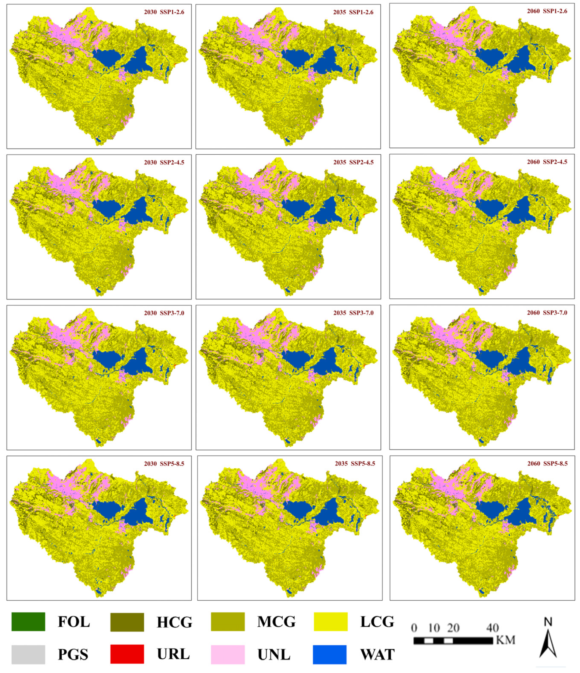
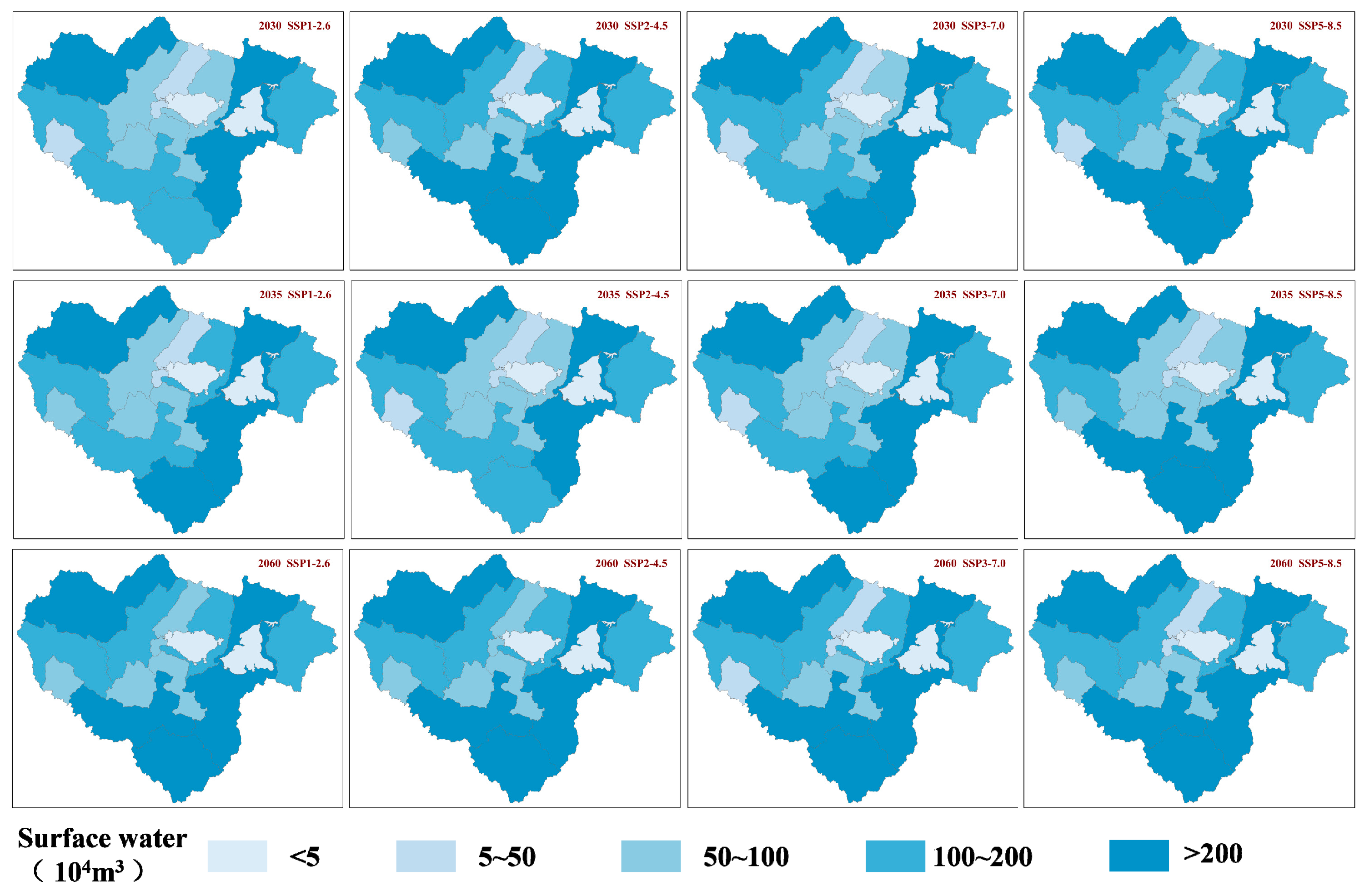
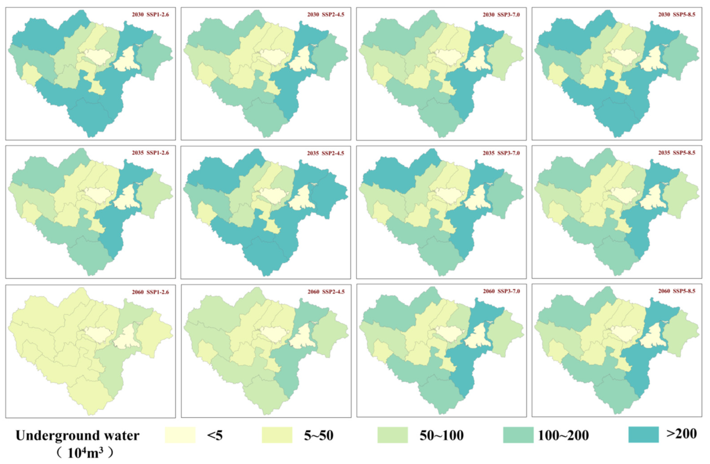
As described in Section 2.4.3, based on the constructed WLR optimization model, the NSGA-II algorithm was applied for multi-objective optimization. After approximately 300 generations, the algorithm converged, the Pareto front stabilized, and multiple independent runs yielded consistent results. Analysis of the converged Pareto front revealed that all solutions on the front exhibited very small variations across the objective functions, indicating that the Pareto set is highly concentrated and the trade-offs among solutions are negligible. Consequently, we directly selected one solution from the converged Pareto front as the final optimal allocation scheme. The resulting optimal water and land resource allocation schemes and their spatial distributions for the YRSR-HHY under four scenarios (SSP1-2.6, SSP2-4.5, SSP3-7.0, and SSP5-8.5) for 2030, 2035, and 2060 are presented in

Table 6. Results of optimal allocation of water resources (10⁴ m³).

Year	Scenarios	Surface Water	Underground Water	Sum
2030	SSP1-2.6	1494.67	366.33	1860.99
	SSP2-4.5	1652.30	233.86	1886.16
	SSP3-7.0	1652.00	233.08	1885.08
	SSP5-8.5	1668.56	296.52	1965.08
2035	SSP1-2.6	1691.27	215.98	1907.25
	SSP2-4.5	1509.05	378.02	1887.07
	SSP3-7.0	1632.83	267.88	1900.70
	SSP5-8.5	1674.78	251.03	1925.82
2060	SSP1-2.6	1910.02	84.06	1994.09
	SSP2-4.5	1855.78	167.61	2023.40
	SSP3-7.0	1737.44	242.53	1979.97
	SSP5-8.5	1793.37	213.03	2006.40

and

Table 7. Results of optimal allocation of land resources (km²).

Year	Scenarios	FOL	HCG	MCG	LCG	WAT	PGS	URL	UNL
2030	SSP1-2.6	1.00	932.75	8068.00	8509.50	1517.25	0.75	4.50	1891.25
	SSP2-4.5	1.00	927.25	8117.75	8519.25	1515.50	0.75	5.00	1838.50
	SSP3-7.0	1.00	979.25	7944.00	8544.50	1558.00	0.75	6.25	1891.25
	SSP5-8.5	1.00	984.50	7655.25	8698.75	1646.75	0.75	4.00	1934.00
2035	SSP1-2.6	1.00	923.25	8026.75	8477.50	1595.50	0.75	4.25	1896.00
	SSP2-4.5	1.00	971.75	8308.75	8187.00	1554.50	0.75	4.50	1896.75
	SSP3-7.0	1.00	941.00	8059.75	8487.50	1569.00	0.75	5.50	1860.50
	SSP5-8.5	1.00	922.25	8124.75	8416.25	1583.50	0.75	4.50	1872.00
2060	SSP1-2.6	1.00	979.75	8500.00	8112.75	1555.00	0.75	5.50	1770.25
	SSP2-4.5	1.00	951.25	8174.00	8523.75	1586.50	0.75	5.50	1682.25
	SSP3-7.0	1.00	996.50	8437.75	8071.50	1631.75	0.75	4.50	1781.25
	SSP5-8.5	1.00	981.75	8356.75	8161.00	1660.25	0.75	4.25	1759.25

, and Figure 13, Figure 14 and Figure 15.

Under different scenarios, the surface water supply for the YRSR-HHY in 2030, 2035, and 2060 ranges from 14.9467 to 16.6856 million m³, 15.0904–16.9127 million m³, and 17.3744–19.1002 million m³, respectively. The corresponding groundwater supply ranges from 2.3308 to 3.6632 million m³, 2.1598–3.7802 million m³, and 0.8406–2.4253 million m³. Both surface water and groundwater supplies show varying degrees of increase across future scenarios. Spatially, the distribution of surface and groundwater resources exhibits similar characteristics across planning years and climate scenarios, following a pattern of “higher in the south than in the north, and greater in the east than in the west.” Areas with higher water supply are primarily concentrated in the downstream regions of the basin. The dynamic changes in surface and groundwater resources ensure water availability for domestic, ecological, and production uses throughout the basin.

Regarding land resource allocation under different scenarios for 2030, 2035, and 2060, compared to the pre-allocation state, FOL and PGS areas show no significant changes. URL and UNL areas decrease by 4.8–14.1% and 2.9–9.7%, respectively. Grassland area increases by 0.4–1.1%, with HCG showing a notable increase of 1.1–4.6%. WAT area decreases by 0.7% and 1.8% in 2030 and 2035, respectively, but increases by 0.2% in 2060. Spatially (Figure 15), the distribution of land use types under future climate scenarios shows no significant differences from the baseline pattern, with the most notable changes being the expansion of WAT near the basin outlet and an increase in MCG area in the southeastern region. Notably, the increase in HCG area is most pronounced under the SSP3-7.0 scenario, with an average expansion of 3.2% across the three target years—substantially higher than under the other scenarios (1.5–2.4%). This aligns with the marked warming projected under SSP3-7.0, which alleviates thermal constraints on vegetation growth and facilitates the transition to higher-coverage grasslands in this alpine region (see Section 4.3 for further details).

After implementing the optimal WLR allocation, no water shortages occur in the YRSR-HHY under any of the four climate scenarios (SSP1-2.6, SSP2-4.5, SSP3-7.0, SSP5-8.5) in 2030, 2035, or 2060. Post-allocation WCC increases by 12.9–20.2% in 2030, 4.6–13.4% in 2035, and 4.6–13.4% in 2060 compared to pre-allocation levels. The WUE improves by 0.6–5.1% in 2030, 4.7–10.7% in 2035, and 4.8–5.2% in 2060. The SEA decreases by 3.9–5.8% in 2030, 4.3–5.8% in 2035, and 7.3–9.1% in 2060 relative to pre-allocation conditions (Figure 16). These results suggest that, under the considered scenarios, all objectives of the WLR optimization were effectively enhanced.

Beyond the individual improvements, the multi-objective allocation reveals important trade-off and synergy patterns among the four ecological targets. Across all scenarios and years, the results reveal a strong synergistic relationship between WCC enhancement and SEA reduction. This indicates that measures promoting water conservation concurrently strengthen soil retention, likely due to the shared benefits of increased vegetation cover. In contrast, the relationship between WUE improvement and WCC enhancement exhibits scenario-dependent characteristics. For instance, under the SSP5-8.5 scenario in 2060, a slight trade-off emerges: while WCC increases by 11.2%, WUE improves by only 4.8%—the smallest gain among all scenarios. This may be explained by the extreme warming–wetting conditions under SSP5-8.5, where accelerated vegetation growth and associated transpiration partially offset the gains in water conservation. Such context-specific trade-offs underscore the necessity of multi-scenario, multi-objective planning to achieve balanced ecological benefits under diverse future climates.

It is worth noting that although total water supply exceeded total demand at the basin level prior to optimization in most scenarios, the optimization still holds significant scientific and management value. First, water resources are unevenly distributed across space, with structural differences among the 14 allocation units; the optimization scheme addresses localized imbalances through cross-unit water reallocation, rather than simply increasing total supply. Second, the water shortage minimization objective serves as a “constraint mechanism” within the multi-objective optimization framework. Without this objective, the algorithm might pursue excessive ecological benefits (e.g., unlimited expansion of high-coverage grassland) at the expense of local water supply–demand balance. Thus, the water shortage minimization objective ensures that the optimized scheme enhances ecological functions while safeguarding basic water security across all units. In summary, the value of optimization lies in spatial allocation and multi-objective synergy, rather than merely addressing aggregate water scarcity.

4. Discussion

4.1. Analysis of the Unique Characteristics and Evolution of WLR in Alpine Plateau Regions

Alpine plateau regions are characterized by high altitude (and often high latitude) and climatic conditions marked by cold and aridity. These compounded environmental constraints result in challenging living conditions and relatively limited human activities. Compared to regions with intensive human disturbance, built-up land occupies a notably smaller proportion of the total area, while alpine grasslands (including meadows) dominate the landscape. This distinct land use structure leads to different developmental priorities, with alpine regions placing greater emphasis on the protection and enhancement of ecological functions. From a water resources perspective, these areas exhibit diverse water phases, most notably abundant solid water reserves in the form of glaciers and permafrost. The transformation between water phases and the associated energy transfer drive changes in soil conditions and vegetation growth states, which further alter the scale, pattern, and quality of vegetation. Concurrently, land use changes feedback into water resource dynamics, collectively driving the evolution of WLR, a process closely linked to regional climate change.

Research indicates that climate change is a key factor influencing runoff generation mechanisms in river basins [30]. The unique runoff composition in the YRSR-HHY—comprising rainfall, glacial meltwater, and baseflow—responds sensitively to climate change and associated glacier–snow–permafrost degradation processes [31,32]. Zhang et al. [33] found that rainfall and glacial-snow melt are the two most influential components of runoff variation in the Yellow River Source Region, contributing approximately 50% and 20%, respectively. Inspired by this, analysis of station observation data from 2000 to 2020 in the YRSR-HHY reveals increasing trends in rainfall and snowfall at rates of 2.3 mm/yr and 2.6 mm/yr, respectively, while temperature exhibited a modest increasing trend of 0.041 °C/yr over the 1980–2020 period, with the increase during 2000–2020 being relatively gradual compared to the baseline period 1980–1999. The contribution of temperature-induced evapotranspiration increase remained minimal during this period. Additionally, permafrost thaw significantly contributes to baseflow. Studies show that permafrost temperatures have generally risen in the Yellow River Source Region, with shallow, cold permafrost warming at faster rates [34]. Accelerated permafrost melting enhances soil permeability, allowing surface runoff to recharge groundwater and form baseflow [35], which may explain the increasing runoff trend observed in the YRSR-HHY over the past two decades.

Climate change, soil conditions, and anthropogenic activities jointly drive land use succession in the basin. Warming and increased moisture have improved local hydrothermal conditions. In alpine regions, medium- and high-coverage grasslands exhibit strong sensitivity to precipitation and temperature, with a particularly positive response to precipitation [36]. Increased precipitation elevates soil carbon, ammonium nitrogen, and total nitrogen content, thereby enhancing grassland coverage and productivity [37]. Ecological conservation initiatives in the Three-Rivers Source Region—including protection projects, grazing exclusion, and ecological restoration—have significantly improved land use efficiency and mitigated grassland degradation [38]. These factors likely explain the observed transition from unused land to low-coverage grassland and the overall expansion of grassland area in the basin.

Existing studies confirm that precipitation in this region is strongly influenced by atmospheric circulation and the East Asian and South Asian monsoons. Under the SSP1-2.6 and SSP2-4.5 scenarios, for example, annual precipitation in the Yellow River Source Region is projected to increase by 11.6% and 11.5%, respectively, over the next 40 years, with precipitation increasing at a rate of 6.0–12.0 mm per decade. Annual runoff is also expected to rise [39,40]. Abundant precipitation and sufficient runoff provide ample water resources for socioeconomic development and ecological construction in the basin. Increased water supply improves local moisture conditions, which is particularly crucial for grassland growth in the region. Simultaneously, higher precipitation increases soil moisture, while climate warming raises soil temperature. These combined improvements favor root development, promote grassland regeneration and expansion, and contribute to effective ecological restoration. As grassland productivity and vegetation coverage increase, the expansion of grassland area becomes a natural outcome.

4.2. Analysis of the Improvement Effect of Different Configuration Objectives

The YRSR-HHY is situated in the core area of the Yellow River ecological barrier and the complex erosion zone of the Qinghai–Tibet Plateau, representing a critical water conservation area, ecological functional zone, and a typical ecologically fragile region [41,42]. This study achieved differentiated ecological benefits in the YRSR-HHY through a multi-objective optimization model. The results indicate that under identical climate scenarios, the optimization scheme yielded varying degrees of improvement across different objectives. Overall, across the four scenarios (SSP1-2.6, SSP2-4.5, SSP3-7.0, and SSP5-8.5), the most substantial enhancement was observed for WCC, with improvement magnitudes of 9.6–17.0%, followed by the reduction in the SEA, with improvements of 5.7–6.6%. In contrast, the enhancement of WUE was relatively limited, ranging from 3.5% to 6.7%.

This differential response can likely be attributed to the varying sensitivities of WCC, SEA, and WUE to climate change and land cover modifications, and is closely related to the intrinsic mechanisms and external drivers of the plateau ecosystem. Comparisons with existing studies can further elucidate the scientific implications. The most substantial improvement in WCC is primarily attributable to the synergistic optimization of altered precipitation patterns and vegetation structure. Projected increases in precipitation directly elevate surface runoff by raising water levels and expanding the area of rivers and lakes, positively impacting short-term water conservation [43]. Notably, the targeted expansion of HCG in the optimized scheme played a crucial role. The increase in HCG area through allocation was particularly effective, as grassland ecosystems with developed root systems and litter layers significantly enhance soil infiltration and water retention capacity [44,45]. Concurrently, grassland expansion improves soil structure, enhances permeability, and promotes groundwater recharge and soil moisture content, contributing to the long-term sustainability of WCC [46]. These findings are largely consistent with the trends in overall grassland area change and WCC on the Qinghai–Tibet Plateau under the future climate scenarios reported by Zhang et al. (2023) [47].

The relatively moderate improvement in SEA reduction reflects the complexity and hysteresis of erosion processes, which can be explained by the inherent characteristics of soil erosion. Soil erosion is a cumulative process significantly influenced by climatic factors such as rainfall intensity, and its full response to configuration optimization may require a longer time to manifest. Although the optimized allocation significantly increased vegetation coverage, the sensitivity of soil erosion to climatic drivers partially offset the improvement effects. Compared to the 5.7–6.6% reduction observed in this study, vegetation restoration and terracing projects on the Loess Plateau achieved substantially higher erosion reductions of 19.4–51.2% [48]. This disparity highlights the unique challenges of ecological restoration in high-altitude cold regions. While increased vegetation coverage enhances soil anti-erodibility, its full protective effect requires time to establish, particularly in this region, characterized by complex erosion types including wind, water, and freeze–thaw erosion. Furthermore, the climate-induced intensification of freeze–thaw cycles and increased rainfall erosivity may counteract some benefits of vegetation restoration [49], resulting in the observed moderate improvement post-allocation.

Meanwhile, this disparity highlights a critical distinction between alpine and loess regions: in high-altitude cold environments, the establishment of vegetation cover is slower and more constrained by thermal conditions, and the persistence of the freeze–thaw cycles continues to mobilize soil even under improved vegetation cover. Consequently, soil erosion control in alpine regions requires longer-term strategies that integrate vegetation restoration with measures addressing freeze–thaw dynamics, rather than relying solely on cover improvement.

The weak response of WUE reveals the limited adaptability of physio-ecological processes to rapid climate change. Climate warming disrupts the land–atmosphere–energy balance, impacting regional ecosystems, with particularly significant effects in high-altitude, high-latitude regions like the Yellow River Source Region [50]. Studies indicate a negative correlation between WUE and both temperature and precipitation in most grassland ecosystems of this region [51], primarily because increased precipitation and temperature jointly exacerbate water loss through evapotranspiration, while productivity changes are relatively smaller, leading to decreased WUE [52]. This is consistent with the relatively limited improvement in WUE observed in our optimization results. Consequently, future vegetation might adapt to the new hydrothermal conditions by adjusting physiological processes such as stomatal regulation, transpiration, and photosynthesis to enhance dry matter accumulation, thereby altering WUE in response to climate change.

The differential responses observed among the three ecological objectives have important implications for water resources’ management. The strong synergy between WCC and SEA suggests that investments in vegetation restoration can yield co-benefits for both water retention and soil conservation, a particularly valuable insight for resource-constrained management agencies. Conversely, the limited and scenario-dependent response of WUE indicates that relying on WUE as a standalone indicator of ecosystem health may be misleading under rapid climate change. Managers should therefore prioritize WCC and SEA as primary targets for intervention, while using WUE as a diagnostic tool to monitor ecosystem stress rather than as a direct performance metric.

The enhancement of all objectives reflects not only climatic influences but also the regulatory role of human activities. Despite challenges like rodent and insect pests, the implementation of ecological conservation projects—including black soil beach restoration, grazing exclusion, and reseeding—has gradually mitigated ecological degradation in the basin [53,54]. These context-specific vegetation restoration measures collectively contribute to the improvement in the basin’s ecological environment quality.

It is crucial to emphasize that the differential responses of the objectives not only reflect inherent differences in natural processes but also highlight the necessity of multi-objective synergistic management. Compared to single-objective optimization, the synergistic allocation scheme in this study achieved soil erosion control while ensuring water conservation, demonstrating that “trade-offs and synergies” are a core characteristic of ecosystem management, even if the degree of improvement varies across objectives. Future research should focus on the response trajectories of various ecological processes across different temporal scales to further enhance the sustainability of optimization schemes.

It is worth reiterating that the value of optimization in this study lies not only in the enhancement of ecological functions, but also in the optimization of spatial water allocation and the constraint mechanism for multi-objective synergy. Although the basin as a whole maintains a supply surplus, cross-unit water reallocation addresses localized structural imbalances. Meanwhile, the water shortage minimization objective serves as a constraint, ensuring that the pursuit of ecological benefits does not compromise basic water security across all units. Thus, the optimization framework achieves a dual improvement: spatial allocation and objective synergy.

4.3. Analysis of Response to Future Climate Scenarios

The YRSR-HHY, located in the northeastern part of the Qinghai–Tibet Plateau, represents a classic climate change hotspot and a pivotal region that is sensitive to environmental shifts across Asia, the Northern Hemisphere, and even globally [55]. Differences in future climate scenarios will lead to varying climate change response capacities within the basin. The IPCC AR6 report utilizes the new Shared Socioeconomic Pathways (SSPs) as a foundation for projecting greenhouse gas emissions and concentrations, combined with Representative Concentration Pathways (RCPs), to describe potential warming trajectories and associated mitigation measures [56,57]. Among these, the SSP3-7.0 scenario integrates the SSP3 narrative (“High challenges to mitigation and adaptation”) with the RCP7.0 forcing level. This pathway is comparatively more pessimistic than the other three scenarios, assuming a lower prioritization of environmental issues and consequently more severe environmental degradation.

However, analysis of the average improvement levels for each objective across the three target years (2030, 2035, 2060) under the four climate scenarios reveals that the optimization schemes enhance all objectives in the YRSR-HHY across all future climates. Notably, the schemes demonstrate pronounced effectiveness even under the medium-to-high radiative forcing of SSP3-7.0. Specifically for WCC enhancement and SEA reduction, the improvements under this scenario are approximately 17.0% and 6.6%, respectively, representing the most significant gains among all scenarios. Although the SSP3 pathway typically entails substantial land use changes (particularly global forest loss) and high climate forcing, the optimized allocation schemes under this scenario still result in an increased combined coverage of forest and grassland compared to both the pre-allocation state and the baseline year. This outcome aligns with the findings from Fan et al. (2023) [58], who reported potential grassland expansion under various future climate scenarios.

The likely explanation for this lies in the distinct characteristics of the SSP3-7.0 scenario. Research indicates that under SSP3-7.0, precipitation increases are relatively modest, while temperature rises are more pronounced [59]. This pattern is markedly evident in the YRSR-HHY, where the mean annual temperature under this scenario is projected to rise to −1.65 °C, a 47.6% increase relative to the 2020 average. This warming, coupled with a reduction in extremely cold days, can alleviate temperature constraints that previously limited vegetation growth in high-altitude cold regions, thereby expanding the potential growing area [60]. Furthermore, higher temperatures accelerate the melting of glaciers, snow, and permafrost, increasing soil moisture availability. This also facilitates the decomposition of soil organic matter, elevating soil carbon content and creating more favorable conditions for root development [61]. Additionally, increased accumulated temperature and a prolonged growing season enable plants to complete their growth cycles more effectively. These combined factors promote vegetation growth and expansion, thereby enhancing ecosystem NPP and effectively mitigating soil erosion [62,63].

The consistent effectiveness under the more challenging SSP3-7.0 scenario suggests that the proposed allocation framework may offer adaptive benefits under a range of climate futures. From a management perspective, this suggests that investments in ecological restoration and water infrastructure could be considered even under more pessimistic climate futures, potentially reducing the risk of maladaptation.

Several management recommendations emerge from these findings. First, priority could be given to expanding high-coverage grassland in areas where thermal conditions are projected to improve, as this yields the greatest co-benefits for WCC and SEA. This recommendation is consistent with national policies, such as the Yellow River Basin Ecological and Environmental Protection Plan, which explicitly calls for “effectively restoring important ecosystems such as alpine meadows, grasslands, wetlands, and forests in water conservation areas, and strengthening water conservation functions.” Second, water allocation strategies should maintain flexibility to accommodate scenario-driven variations in surface water and groundwater availability; for instance, under SSP5-8.5, the substantial increase in surface water supply (Table 6) could support targeted ecological water replenishment during dry seasons. Third, given the limited WUE response under extreme warming, managers should avoid over-reliance on WUE-based performance targets and instead focus on direct measures of ecosystem structure (vegetation cover) and function (water conservation, soil retention). Finally, the observed trade-off between WCC and WUE under SSP5-8.5 underscores the need for adaptive management frameworks that can adjust priorities as climate conditions evolve, rather than adhering to fixed targets.

These findings also have relevance beyond the study region. Many high-mountain watersheds across the Hindu Kush Himalaya, Andes, and other alpine zones face similar challenges of climate-induced cryosphere change and ecological vulnerability. The multi-objective framework developed here, with its emphasis on ecological function enhancement and consistency across scenarios, offers a transferable conceptual framework for climate adaptation planning in these regions, although direct operational application would require calibration to local conditions.

This study has the following limitations. First, climate scenario projections involve uncertainty; although CMIP6 outputs were bias-corrected, differences in model structure remain. Future research could consider multi-model ensemble averaging to reduce uncertainty. Second, regarding the representativeness of WUE as an ecological target, while WUE is an important indicator of vegetation water use efficiency, a single indicator cannot fully capture ecosystem health; additional ecological indicators could be incorporated in future studies. Third, the optimization framework does not consider policy implementation costs; practical application would require integration with socioeconomic feasibility assessments. Fourth, although model parameters were validated against historical data, a full uncertainty analysis is lacking. Fifth, future research could further quantitatively separate the contributions of climate forcing and land use changes to NPP dynamics to more deeply elucidate the driving mechanisms of regional vegetation change. Nonetheless, the framework and methods presented in this study provide a scientific reference for water and land resource management in alpine regions.

5. Conclusions

This study focused on the YRSR-HHY. Through a systematic analysis of the historical evolution of water–land resources, a multi-objective optimization model for their allocation, oriented towards ecological function enhancement, was developed. Future allocation schemes were simulated and evaluated under multiple climate scenarios. The main conclusions are as follows:

(1)

Over the past two decades, the study area has exhibited a pronounced “warming–wetting” trend, accompanied by positive changes in the water–land resource system and ecological quality. Specifically, surface water and groundwater resources increased at rates of 54 million m³/year and 30 million m³/year, respectively. Land use type transitions occurred across 23.6% of the area, primarily involving the conversion of 3456.80 km² of unused land to low-coverage grassland. The basin’s NPP and WCC increased at annual rates of 1.56 kg C/km² and 0.025 mm, respectively, while the SEA decreased at a rate of 0.036 t/(hm²·5a).

(2)

There is an urgent need to enhance future ecological functions. Projections indicate that without optimal allocation, the basin’s WUE would change by −4.2% to 6.9%, WCC by −1.6% to 6.3%, while the SEA would increase by 10.3% to 36.0% under different climate scenarios. This reflects the inadequacy of the current water–land resources pattern in adapting to future climate change.

(3)

The multi-objective optimal allocation demonstrated significant effectiveness. The allocation schemes obtained by constructing a water–land resources system network and employing the NSGA-II algorithm achieved comprehensive improvement in ecological functions across all climate scenarios: the WCC increased by 4.6–20.2%, the WUE improved by 0.6–10.7%, and the SEA decreased by 3.9–9.1%. It is particularly noteworthy that the allocation schemes exhibited consistent effectiveness even under the more challenging SSP3-7.0 scenario, suggesting potential for adaptation under a range of climate futures.

It should be noted that this study has certain limitations. Factors such as implementation costs were not taken into account in the climate scenario projections, model parameter settings, and optimization framework, which may affect the generalizability of the results. Therefore, for practical applications, it is recommended that optimization schemes be calibrated based on specific local conditions, and that future studies incorporate a more comprehensive uncertainty analysis.

References

1. Hou, Y.; Zhao, W.; Liu, Y.; Yang, S.; Hu, X.; Cherubini, F. Relationships of multiple landscape services and their influencing factors on the Qinghai-Tibet Plateau. Landsc. Ecol. 2021, 36, 1987–2005. [Google Scholar] [CrossRef]
2. Zhu, L.; Yang, M.; Liu, J.; Zhang, Y.; Li, B.; Zhou, B.; Chen, X. The influence of permafrost degradation on the change of suprapermafrost water: A case study in the source areaof the Yellow River. Hydrogeol. Eng. Geol. 2023, 50, 3–13. [Google Scholar]
3. Zhang, T.; Cheng, C.; Shen, S. Quantifying ecosystem quality in the Tibetan Plateau through a comprehensive assessment index. Environ. Sustain. Indic. 2024, 22, 100382. [Google Scholar] [CrossRef]
4. Kraaijenbrink, P.D.A.; Bierkens, M.F.P.; Lutz, A.F.; Immerzeel, W.W. Impact of a global temperature rise of 1.5 degrees Celsius on Asia’s glaciers. Nature 2017, 549, 257–260. [Google Scholar] [CrossRef]
5. Ding, Y.; Zhang, S.; Zhao, L.; Li, Z.; Kang, S. Global warming weakening the inherent stability of glaciers and permafrost. Sci. Bull. 2019, 64, 245–253. [Google Scholar] [CrossRef]
6. Xu, F.; Zhang, G.; Woolway, R.I.; Yang, K.; Wada, Y.; Wang, J.; Cretaux, J.-F. Widespread societal and ecological impacts from projected Tibetan Plateau lake expansion. Nat. Geosci. 2024, 17, 516–523. [Google Scholar] [CrossRef]
7. Jin, X.; Jin, H.; Luo, D.; Sheng, Y.; Wu, Q.; Wu, J.; Wang, W.; Huang, S.; Li, X.; Liang, S.; et al. Impacts of Permafrost Degradation on Hydrology and Vegetation in the Source Area of the Yellow River on Northeastern Qinghai-Tibet Plateau, Southwest China. Front. Earth Sci. 2022, 10, 845824. [Google Scholar] [CrossRef]
8. Wang, A.; Lv, W.; Zhou, Y.; Li, B.; Sun, J.; Lv, J.; Chen, L.; Tsecheo, D.; Wang, S. Drought decreases the positive impact of warming on an alpine grassland community. Sci. China Earth Sci. 2024, 67, 3226–3238. [Google Scholar] [CrossRef]
9. Yang, A.; Zhang, H.; Yang, X.; Zhang, X. Quantitative analysis of the impact of climate change and human activities on vegetation NPP in the Qilian Mountain. Hum. Ecol. Risk Assess. 2023, 29, 202–221. [Google Scholar] [CrossRef]
10. Grantham, T.E.W.; Carlisle, D.M.; McCabe, G.J.; Howard, J.K. Sensitivity of streamflow to climate change in California. Clim. Change 2018, 149, 427–441. [Google Scholar] [CrossRef]
11. Yang, J.; Chang, J.; Yao, J.; Wang, Y.; Huang, Q.; Xu, G. Impact of natural climate variability on runoff based on Monte Carlo method. J. Water Clim. Change 2019, 10, 344–359. [Google Scholar] [CrossRef]
12. Yu, D.; Liu, Y.; Xie, D.; Mu, C.; Sun, Z.; Zhou, M.; Rao, J.; Suolang, D.; Xiong, Y.; Chen, J.-S. Effects of driving factors on water supply function under different basins and spatial scale in Zoige alpine wetland, China. Ecol. Indic. 2024, 158, 111403. [Google Scholar] [CrossRef]
13. Gautam, V.K.; Awasthi, M.K.; Trivedi, A. Optimum allocation of water and land resource for maximizing farm income of Jabalpur District, Madhya Pradesh. Int. J. Environ. Clim. Change 2020, 10, 224–232. [Google Scholar] [CrossRef]
14. Wang, Y.; Guo, S.; Yue, Q.; Mao, X.; Guo, P. Distributed AquaCrop simulation-nonlinear multi-objective dependent-chance programming for irrigation water resources management under uncertainty. Agric. Water Manag. 2021, 247, 106752. [Google Scholar] [CrossRef]
15. Cheng, H.; Jiang, X.; Wang, M.; Zhu, T.; Wang, L.; Miao, L.; Chen, X.; Qiu, J.; Shu, J.; Cheng, J. Optimal allocation of agricultural water and land resources integrated with virtual water trade: A perspective on spatial virtual water coordination. J. Environ. Manag. 2023, 347, 119189. [Google Scholar] [CrossRef]
16. Wang, J.; Qin, T.; Lv, X.; Ni, Y.; Zhang, Q.; Ma, L. Study of Optimal and Joint Allocations of Water and land Resources for Multiple Objectives. Water Resour. Manag. 2023, 37, 1241–1256. [Google Scholar] [CrossRef]
17. Qin, T.; Feng, J.; Li, C.; Zhang, X.; Yan, D.; Liu, S.; Wang, J.; Lv, X.; Abebe, S.A. Risk assessment and configuration of water and land resources system network in the Huang-Huai-Hai watershed. Ecol. Indic. 2023, 154, 110712. [Google Scholar] [CrossRef]
18. Lu, N.; Zhang, J.; Su, C.; Hu, Z.; Wu, Z.; Yan, D. Joint optimal allocation of regional water and land resources considering mutual feedback relationship. Adv. Water Sci. 2024, 35, 208–219. [Google Scholar] [CrossRef]
19. Jin, S.; Su, C.; Huang, J.; Wang, H.; Yan, D.; Wang, Z. Joint optimal allocation of regional water and land resources in response to ecological-economic-social demands. Water Resour. Hydropower Eng. 2025, 56, 61. [Google Scholar]
20. Su, C.; Hu, Z.; Yuan, W.; Zhang, J.; Yan, D.; Wang, H. Joint optimal allocation of regional water and land resources considering their mutual feed relationship. J. Hydrol. 2024, 638, 131492. [Google Scholar] [CrossRef]
21. Li, W.; Weng, B.; Yan, D.; Lai, Y.; Li, M.; Wang, H. Underestimated permafrost degradation: Improving the TTOP model based on soil thermal conductivity. Sci. Total Environ. 2022, 854, 158564. [Google Scholar] [CrossRef]
22. Guo, Q.; Yu, C.; Xu, Z.; Yang, Y.; Wang, X. Impacts of climate and land-use changes on water yields: Similarities and differences among typical watersheds distributed throughout China. J. Hydrol. Reg. Stud. 2023, 45, 101294. [Google Scholar] [CrossRef]
23. Zheng, G.; Li, C.; Li, R.; Luo, J.; Fan, C.; Zhu, H. Spatio-temporal evolution analysis of landscape pattern and habitat quality in the Qinghai Province section of the Yellow River Basin from 2000 to 2022 based on InVEST model. J. Arid. Land 2024, 16, 1183–1196. [Google Scholar] [CrossRef]
24. Pathak, S.; Ojha, C.S.P.; Garg, R.D. Applicability of the InVEST Model for Estimating Water Yield in Upper Ganga Basin. In The Ganga River Basin: A Hydrometeorological Approach; Springer International Publishing: Cham, Switzerland, 2021; pp. 219–231. [Google Scholar]
25. Xiang, S.; Xiong, K.; Zhang, B.; Li, Y.; Zhang, W.; Li, R. Spatiotemporal dynamics and driving mechanisms of grassland landscape fragmentation in China’s karst regions. Ecol. Indic. 2025, 179, 114185. [Google Scholar] [CrossRef]
26. Alhamad, M.N.; Alrababah, M.A.; Feagin, R.A.; Gharaibeh, A. Mediterranean drylands: The effect of grain size and domain of scale on landscape metrics. Ecol. Indic. 2011, 11, 611–621. [Google Scholar] [CrossRef]
27. Teng, M.J.; Zeng, L.X.; Zhou, Z.X.; Wang, P.C.; Xiao, W.F.; Dian, Y.Y. Responses of landscape metrics to altering grain size in the Three Gorges Reservoir landscape in China. Environ. Earth Sci. 2016, 75, 1055. [Google Scholar] [CrossRef]
28. Yan, Y.Z.; Jarvie, S.; Zhang, Q.; Zhang, S.S.; Han, P.; Liu, Q.F.; Liu, P.T. Small patches are hotspots for biodiversity conservation in fragmented landscapes. Ecol. Indic. 2021, 130, 108086. [Google Scholar] [CrossRef]
29. Gao, H.; Qin, T.; Luan, Q.; Feng, J.; Zhang, X.; Yang, Y.; Xu, S.; Lu, J. Characteristics Analysis and Prediction of Land Use Evolution in the Source Region of the Yangtze River and Yellow River Based on Improved FLUS Model. Land 2024, 13, 393. [Google Scholar] [CrossRef]
30. Pan, Z.; Liu, P.; Gao, S.; Xia, J.; Chen, J.; Cheng, L. Improving hydrological projection performance under contrasting climatic conditions using spatial coherence through a hierarchical Bayesian regression framework. Hydrol. Earth Syst. Sci. 2019, 23, 3405–3421. [Google Scholar] [CrossRef]
31. Immerzeel, W.W.; Lutz, A.F.; Andrade, M.; Bahl, A.; Biemans, H.; Bolch, T.; Hyde, S.; Brumby, S.; Davies, B.J.; Elmore, A.C.; et al. Importance and vulnerability of the world’s water towers. Nature 2020, 577, 364–369. [Google Scholar] [CrossRef]
32. Wang, T.; Zhao, Y.; Xu, C.; Ciais, P.; Liu, D.; Yang, H.; Piao, S.; Yao, T. Atmospheric dynamic constraints on Tibetan Plateau freshwater under Paris climate targets. Nat. Clim. Change 2021, 11, 219–225. [Google Scholar] [CrossRef]
33. Zhang, T.; Li, D.; Lu, X. Response of runoff components to climate change in the source-region of the Yellow River on the Tibetan plateau. Hydrol. Process. 2022, 36, e14633. [Google Scholar] [CrossRef]
34. Luo, D.; Jin, H.; Jin, X.; He, R.; Li, X.; Muskett, R.R.; Marchenko, S.S.; Romanovsky, V.E. Elevation-dependent thermal regime and dynamics of frozen ground in the Bayan Har Mountains, northeastern Qinghai-Tibet Plateau, southwest China. Permafr. Periglac. Process. 2018, 29, 257–270. [Google Scholar] [CrossRef]
35. Qin, Y.; Yang, D.; Gao, B.; Wang, T.; Chen, J.; Chen, Y.; Wang, Y.; Zheng, G. Impacts of climate warming on the frozen ground and eco-hydrology in the Yellow River source region, China. Sci. Total Environ. 2017, 605, 830–841. [Google Scholar] [CrossRef]
36. Hou, Q.; Yang, H.; Wu, J.; Yu, X. Carbon budget response to climate change varies with grassland type in Qilian Mountains, China. Glob. Ecol. Conserv. 2023, 47, e02670. [Google Scholar] [CrossRef]
37. Wang, Y.; Lv, W.; Xue, K.; Wang, S.; Zhang, L.; Hu, R.; Zeng, H.; Xu, X.; Li, Y.; Jiang, L.; et al. Grassland changes and adaptive management on the Qinghai-Tibetan Plateau. Nat. Rev. Earth Environ. 2022, 3, 668–683. [Google Scholar] [CrossRef]
38. Shao, Q.; Liu, J.; Huang, L.; Fan, J.; Xu, X.; Wang, J. Integrated assessment on the effectiveness of ecological conservation in Sanjiangyuan National Nature Reserve. Geogr. Res. 2013, 32, 1645–1656. [Google Scholar] [CrossRef]
39. Liu, Y.; Gao, G.; Zhai, J.; Liu, L.; Wen, T.; Sun, Y. The discharge change in the source region of the Yellow River in the next 40 years based on the CMIP6 and two hydrological models. J. Glaciol. Geocryol. 2024, 46, 675–687. [Google Scholar] [CrossRef]
40. Jia, H.; Li, X.; Wen, J.; Chen, Y. Runoff change simulation and future trend projection in the source area of the Yellow River. Resour. Sci. 2022, 44, 1292–1304. [Google Scholar] [CrossRef]
41. Li, C.; Hao, Y.; Zheng, Z.; Xu, X.; Cui, L.; Guan, M.; Guan, S.; Li, T.; Pang, Z.; Li, L.; et al. Determination of priority conservation areas in the Yellow River source region based on ecosystem integrity evaluations. Glob. Ecol. Conserv. 2024, 49, e02800. [Google Scholar] [CrossRef]
42. Zhang, H.; Song, Q.; Zhao, J.; Liu, P.; Lu, Z.; Wang, S. Application of the New Assessment Framework in the Identification of Key Areas for Ecological Protection: A Case Study of the Yellow River Source Area on the Tibetan Plateau. Geocarto Int. 2023, 38, 2292748. [Google Scholar] [CrossRef]
43. Zhang, Y.; Zhou, D.; Guo, X. Regional climate response to global warming in the source region of the Yellow River and its impact on runoff. Sci. China Earth Sci. 2024, 67, 843–855. [Google Scholar] [CrossRef]
44. Furtado, M.F.; Valentin, L.Z. Soil water infiltration under different land use conditions: In situ tests and modeling. RBRH-Rev. Bras. Recur. Hídricos 2021, 26, e26. [Google Scholar] [CrossRef]
45. Bialkowski, R.; Buttle, M.J. Soil water recharge for grassed and forested land covers on the Oak Ridges Moraine, southern Ontario, Canada. Hydrol. Res. 2016, 47, 390–408. [Google Scholar] [CrossRef]
46. Zhang, W.; Zhu, R.; Yang, Q.; Shan, J.; Feng, Y.; Yin, Z. Spatio-Temporal Evolution and Prediction of Carbon Storage in the Water Conservation Area of the Yellow River Basin based on the PLUS-InVEST Model. Plateau Meteorol. 2025, 44, 362–377. [Google Scholar] [CrossRef]
47. Zhang, C.; Long, D.; Liu, T.; Slater, L.J.; Wang, G.; Zuo, D.; Duan, L.; Cui, Y.; Cui, Y. Grassland greening and water resource availability may coexist in a warming climate in Northern China and the Tibetan Plateau. Earth’s Future 2023, 11, e2023EF004037. [Google Scholar] [CrossRef]
48. Tian, P.; Tian, X.; Geng, R.; Zhao, G.; Yang, L.; Mu, X.; Gao, P.; Sun, W.; Liu, Y. Response of soil erosion to vegetation restoration and terracing on the Loess Plateau. Catena 2023, 227, 107103. [Google Scholar] [CrossRef]
49. Yao, M.; Yin, J.; Liu, S.; Jiang, Q.; Yuan, Z. Changes of water cycle elements and their ecological effects in source region of Changjiang River and Yellow River under climate change. Yangtze River 2024, 55, 74–82. [Google Scholar] [CrossRef]
50. Hou, B. Analysis of Inter-Relationships Between Climate Change and Runoff discharge in the Headwater Region of Yellow River. Ph.D. Thesis, Beijing Forestry University, Beijing, China, 2020. [Google Scholar] [CrossRef]
51. Lin, Z.; Wen, Z.; Liu, Y.; Yao, H.; Zhou, R.; Ren, H.; Yuan, L. Spatiotemporal variation and attribution of carbon and water use efficiency in the Yellow River Basin based on remote sensing data. Acta Ecol. Sin. 2024, 44, 377–391. [Google Scholar] [CrossRef]
52. Du, X.; Zhao, X.; Wang, H.; He, B. Responses of terrestrial ecosystem water use efficiency to climate change: A review. Acta Ecol. Sin. 2018, 38, 8296–8305. [Google Scholar]
53. Lu, Z.; Song, Q.; Zhao, J. Evolution of Landscape Ecological Risk and Identification of Critical Areas in the Yellow River Source Area Based on LUCC. Sustainability 2023, 15, 9749. [Google Scholar] [CrossRef]
54. Zhu, G.; Gao, H.J.; Zeng, G. Landscape pattern change of sandy desertification land in the source region of the Yellow River during the past 45 years. J. Arid. Land Resour. Environ. 2021, 35, 79–85. [Google Scholar]
55. Luo, H.; Wang, Z.; He, C.; Chen, D.; Yang, S. Future changes in South Asian summer monsoon circulation under global warming: Role of the Tibetan Plateau latent heating. npj Clim. Atmos. Sci. 2024, 7, 103. [Google Scholar] [CrossRef]
56. Wayne, G.P. The beginner’s guide to representative concentration pathways. Skept. Sci. 2013, 25, 1–6. [Google Scholar]
57. Riahi, K.; Van Vuuren, D.P.; Kriegler, E.; Edmonds, J.; O’Neill, B.C.; Fujimori, S.; Bauer, N.; Calvin, K.; Dellink, R.; Fricko, O.; et al. The Shared Socioeconomic Pathways and their energy, land use, and greenhouse gas emissions implications: An overview. Glob. Environ. Change-Hum. Policy Dimens. 2017, 42, 153–168. [Google Scholar] [CrossRef]
58. Fan, M.; Wang, P.; Chen, Y.; Liu, H.; Liu, Y.; Chen, Y.; Gang, C.; Ma, F. Spatial and Temporal Dynamics of Global Grassland and Net Primary Productivity under Different Future Climate Scenarios. Acta Agrestia Sin. 2023, 31, 3597–3607. [Google Scholar] [CrossRef]
59. Shiogama, H.; Fujimori, S.; Hasegawa, T.; Hayashi, M.; Hirabayashi, Y.; Ogura, T.; Iizumi, T.; Takahashi, K.; Takemura, T. Important distinctiveness of SSP3–7.0 for use in impact assessments. Nat. Clim. Change 2023, 13, 1276–1278. [Google Scholar] [CrossRef]
60. Zhang, Q.; Kong, D.; Shi, P.; Singh, V.P.; Sun, P. Vegetation phenology on the Qinghai-Tibetan Plateau and its response to climate change (1982–2013). Agric. For. Meteorol. 2018, 248, 408–417. [Google Scholar] [CrossRef]
61. Liu, Y.; Cui, Z.; Huang, Z.; López-Vicente, M.; Wu, G.L. Influence of soil moisture and plant roots on the soil infiltration capacity at different stages in arid grasslands of China. Catena 2019, 182, 104147. [Google Scholar] [CrossRef]
62. Quan, Q.; Tian, D.; Luo, Y.; Crowther, T.; Zhu, K.; Chen, H.; Zhou, Q.; Niu, S. Water scaling of ecosystem carbon cycle feedback to climate warming. Sci. Adv. 2019, 5, eaav1131. [Google Scholar] [CrossRef]
63. Wei, Y.; Lu, H.; Wang, J.; Wang, X.; Sun, J. Dual Influence of Climate Change and Anthropogenic Activities on the Spatiotemporal Vegetation Dynamics Over the Qinghai-Tibetan Plateau From 1981 to 2015. Earth’s Future 2022, 10, e2021EF002566. [Google Scholar] [CrossRef]
64. Zhang, L.; Hickel, K.; Dawes, W.R.; Chiew, F.H.S.; Western, A.W.; Briggs, P.R. A rational function approach for estimating mean annual evapotranspiration. Water Resour. Res. 2004, 40, W02502. [Google Scholar] [CrossRef]
65. Yang, Y.H.; Zhang, X.Y.; Chen, J.; Qin, T.L.; Xu, S.; Lu, J.; Liu, H.X.; Gao, H.Y. Evolution and influencing factors of water yield and water conservation services in the Yellow River Source Area from 2000 to 2020. Appl. Ecol. Environ. Res. 2023, 21, 4195–4212. [Google Scholar] [CrossRef]
66. Wang, Y.; Zhao, J.; Fu, J.; Wei, W. Effects of the Grain for Green Program on the water ecosystem services in an arid area of China-Using the Shiyang River Basin as an example. Ecol. Indic. 2019, 104, 659–668. [Google Scholar] [CrossRef]
Figure 1. Scientific hypothesis map (in the figure, P is precipitation, T is temperature, R is runoff, E is Evaporation, GS is glacier and snow, R is rainfall, and S is snowfall).
Land 15 00631 g001
Figure 2. Geographical location of the study area. (a) Location of study area; (b) Trend of temperature change in recent forty years; (c) Trend of precipitation change in recent forty years.
Land 15 00631 g002
Figure 3. The technical route of research.
Land 15 00631 g003
Figure 4. Configuration unit division (Numbers 1–14 represent the sequence of configuration units).
Land 15 00631 g004
Figure 5. Total water resources (left) and interannual variation trend of surface water resources and groundwater resources (right).
Land 15 00631 g005
Figure 6. Water supply structure (a) and water use structure (b).
Land 15 00631 g006
Figure 7. Changes in land use composition. The code in the figure consists of year and land use code. The first four digits represent the years of land use, namely, 2000, 2005, 2010, 2015 and 2020, and the last two digits represent land use types, in which 01 is FOL, 02 is HCG, 03 is MCG, 04 is LCG, 05 is WAT, 06 is PGS, 07 is URL and 08 is UNL. Take 200004 as an example to show the area of LCG in the basin in 2000.
Land 15 00631 g007
Figure 8. Spatial distribution pattern of land use and land use transfer patterns. (The land use transfer pattern consists of two numbers: the first number is the land use type in 2000, and the second number is the land use type in 2020).
Land 15 00631 g008
Figure 9. Annual variation trend of NPP: (A) the spatial distribution of main ecological functions (The dashed line in the figure is a linear fitting.); (B) the spatial distribution of WCC; (C) the spatial distribution of SEA.
Land 15 00631 g009
Figure 10. WUE time variation (The dashed line in the figure is a linear fitting) and changes in WUE in different land use types.
Land 15 00631 g010
Figure 11. Changes in water yield coefficient of different land use types.
Land 15 00631 g011
Figure 12. The increase in WCC, SEA and WUE in different years in the future under four climate scenarios is estimated compared with 2020.
Land 15 00631 g012
Figure 13. Surface water supply in different scenarios in 2030, 2035 and 2060 after allocation.
Land 15 00631 g013
Figure 14. Groundwater supply in different scenarios in 2030, 2035 and 2060 after allocation.
Land 15 00631 g014
Figure 15. Spatial distribution of land use in different scenarios in 2030, 2035 and 2060 after allocation.
Land 15 00631 g015
Figure 16. Analysis of optimal allocation effect.
Land 15 00631 g016