Article

Regulating Effects of Blue–Green Spaces on Land Surface Temperature Based on Local Climate Zones: A Case Study of Suzhou (2000–2022)

1
School of Artificial Intelligence, China University of Geosciences (Beijing), Beijing 100083, China
2
Hebei Key Laboratory of Geospatial Digital Twin and Collaborative Optimization, China University of Geosciences (Beijing), Beijing 100083, China
*
Author to whom correspondence should be addressed.
These authors contributed equally to this work.
Land 2026, 15(4), 618; https://doi.org/10.3390/land15040618
Submission received: 16 February 2026 / Revised: 6 April 2026 / Accepted: 7 April 2026 / Published: 9 April 2026
(This article belongs to the Special Issue GeoAI Application in Urban Land Use and Urban Climate)

Abstract

Rapid urbanization has intensified urban surface thermal stress, yet how blue–green spaces (BGs) are associated with land surface temperature (LST) under different urban morphological contexts remains insufficiently understood. Using Suzhou, China, as a case study, this study integrates Landsat imagery from five representative years (2000, 2005, 2010, 2016, and 2022) with a 100 m local climate zone (LCZ) dataset to examine BGs–LST relationships over time. Two BGs indicators are considered: BGs proportion and the within-grid local dispersion of BGs, represented by BGs_std. The results show that LST in Suzhou’s built-up area exhibits a “rise–decline–rise” pattern during the study period, whereas BGs proportions evolve differently across LCZ types. Regression slope analysis shows that higher BGs proportion is generally associated with lower LST across most LCZ types and study years. Relatively stable negative associations are observed in LCZ 2, LCZ 3, LCZ 6, LCZ 9, and LCZ 10. Pearson correlation analysis further shows that BGs_std is generally positively associated with LST and that this relationship tends to strengthen over time. Relatively stronger associations are observed in LCZ 1, LCZ 3, LCZ 5, and LCZ 6 in some years. These findings suggest that BGs–LST relationships should be interpreted not only in terms of BGs proportion, but also in relation to urban form and within-unit BGs organization. This study provides an LCZ-based empirical perspective on BGs–LST associations in the context of a rapidly urbanizing city.

1. Introduction

Since the turn of the 21st century, rapid global urbanization has profoundly altered the physical properties and spatial structure of urban surfaces. The resulting urban heat island effect has emerged as a prominent environmental issue, posing significant threats to both public health and ecological sustainability [1,2]. The urban heat island effect leads to markedly higher temperatures in urban areas than in surrounding suburbs, a phenomenon that not only exacerbates peak summer energy consumption [3] but also increases the risk of heat-related illnesses [4]. Against this backdrop, mitigating thermal stress through scientific urban planning has become a critical challenge and an important focus of contemporary research [5].
Land surface temperature (LST) is a widely used indicator for monitoring urban thermal environments [6,7]. As essential components of urban natural cooling systems, blue–green spaces (BGs)—including water bodies, parks, and green areas—have been shown to effectively reduce local surface temperatures and improve thermal environments through ecological processes such as transpiration, evaporation, and shading [8,9]. However, the cooling effect of BGs does not show a simple linear relationship with their total area. Instead, it is influenced by multiple factors, including local dispersion, landscape patterns, and interactions with the surrounding built environment [10]. For instance, BGs of identical area may yield vastly different cooling outcomes due to variations in morphology, local dispersion, and their relationship with building layouts. Consequently, relying solely on overall BGs coverage is insufficient for more context-sensitive urban planning, and further attention should be given to internal structural characteristics and the spatial organization of BGs.
Current research emphasizes two primary dimensions of BGs influence on urban thermal environments: area and landscape structure. Extensive studies have shown that increased BGs coverage typically correlates with reduced LST [11,12]. Simultaneously, research utilizing landscape indices (e.g., patch size, fragmentation, clustering, and connectivity) indicates that spatial pattern differences significantly affect overall cooling efficiency [13,14,15]. Current research on how the size and structural characteristics of BGs affect the urban thermal environment is relatively well developed. Current research has shown that increasingly converging BGs can reduce LST, enhance cooling performance, and expand the spatial extent of cooling. Both water bodies and vegetation patches can generate significant urban cooling island effects. Further research has shown that the cooling effect of BGs does not increase linearly with area. No universal threshold scale has been identified across different cities and surface types, and beyond a certain size, the cooling effect or cooling extent tends to remain relatively stable. In terms of area, many studies have further shown that the spatial structure of BGs influences cooling efficiency, as reflected by landscape indices. Patch size, shape complexity, degree of fragmentation, and connectivity can all influence cooling intensity and the spatial extent of cooling. In general, larger, more regularly shaped, less fragmented, and better-connected BGs tend to exhibit stronger cooling effects. By contrast, highly fragmented or morphologically complex patches tend to weaken the overall cooling effect.
Crucially, the cooling effect of BGs is closely related to the heterogeneity of the surrounding urban structure [16,17]. To conduct more comparable analyses while controlling for background differences in the built environment [18], the local climate zone (LCZ) classification system proposed by Stewart and Oke (2012) [19] provides a useful research framework [20]. The LCZ system partitions urban areas into distinct types characterized by consistent surface structures, cover materials, and human activities (e.g., Compact high-rise, Open low-rise, Heavy industry), thereby establishing a standardized basis for comparing the thermal regulation of BGs across different urban morphological units. Although recent studies have begun integrating LCZ types to examine urban thermal environments [21], most remain constrained by data availability, making it difficult to elucidate the underlying mechanisms linking BGs patterns to surface temperature dynamics over long time series [22,23,24]. Furthermore, existing research has predominantly focused on BGs area proportion, with insufficient exploration of how the within-grid local dispersion of BGs is associated with LST [25].
To examine BGs–LST relationships under different urban morphological contexts, this study takes Suzhou, China, as a case study. Using a 100 m LCZ dataset spanning 2000–2022, together with multi-period BGs and LST data derived from Google Earth Engine (GEE), it investigates how BGs patterns in different LCZ types were associated with surface thermal conditions over time. The specific objectives of this study are as follows: (1) To characterize the spatiotemporal evolution of LST in Suzhou across five representative years (2000, 2005, 2010, 2016, 2022); (2) to quantify the spatiotemporal variation characteristics of the proportion of BGs within different LCZ types during the five periods; (3) to reveal the direction and strength of the association between BGs proportion and LST under different LCZ types through regression slope analysis; (4) to examine the temporal patterns of the relationship between the within-grid local dispersion of BGs and LST across different LCZ types using Pearson correlation analysis.
This study integrates established approaches on BGs, LCZ types, and LST to examine how BGs proportion and within-grid local dispersion are associated with LST under different urban morphological contexts. Using Suzhou as a case study, it provides stage-based empirical evidence from 2000 to 2022 and extends existing LCZ-based urban climate research to a long-term comparative setting.

2. Materials and Methods

2.1. Study Area

Suzhou is located in the core region of the Yangtze River Delta (approximately 119°55′ E–121°20′ E, 30°47′ N–32°02′ N). As a typical plain-water-network city, Suzhou is characterized by a dense system of lakes and waterways, with abundant blue space resources. From 2000 to 2022, Suzhou experienced sustained rapid urban expansion, with its built-up area continuously extending outward. Consequently, urban land cover shifted significantly from natural and semi-natural surfaces to high-intensity impervious surfaces, leading to increasingly severe surface thermal environment problems [26]. Concurrently, driven by urban renewal and ecological development initiatives, the BGs within the built-up area underwent significant phased adjustments regarding their proportion, morphology, and local dispersion. This evolution involved two concurrent processes: the localized compression and fragmentation of natural areas, alongside the embedding and reorganization of ecological elements such as parks, green spaces, and waterfront areas. Given the diverse built environment types and distinct urban morphologies within the study area, the long-term LCZ framework is highly suitable for conducting comparative analyses of BGs evolution and its relationship with LST from 2000 to 2022 [22]. This framework provides a standardized basis for examining BGs–LST relationships across built-up areas (Figure 1).

2.2. Data

The study period spans from 2000 to 2022 and covers the built-up area of Suzhou. Within this period, five representative years (2000, 2005, 2010, 2016, and 2022) were selected based on urban development stage, temporal representativeness, and data comparability. In the context of Suzhou, 2000 serves as an early baseline year; 2005 and 2010 capture a period of rapid industrialization and urban expansion; 2016 represents a more mature stage marked by increasing spatial restructuring and ecological management; and 2022 reflects the city’s most recent development condition. These five temporal nodes therefore support stage-based long-term comparison while ensuring the consistent integration of BGs, LCZ, and LST data within a unified processing framework. The analysis relies primarily on three datasets: BGs, LST, and LCZ classification data. BGs and LST data were extracted using the GEE platform. LCZ classification data were obtained from the publicly available dataset, “Annual Local Climate Zones at 100-Meter Resolution for China’s Major Cities, 2000–2022”(https://zenodo.org/records/14614256 (accessed on 20 October 2025)) [27].

2.2.1. BGs Data

To construct a consistent long-term BGs dataset, a standardized image processing workflow was established on the GEE platform. Five representative years were selected, and Landsat imagery acquired during the vegetation growing season (1 June to 31 October) was used to maximize the spectral separability of vegetation and water features. For years before 2013, Landsat 5 TM and Landsat 7 ETM+ Collection 2 Level 2 surface reflectance products were used, whereas Landsat 8 OLI Collection 2 Level 2 surface reflectance data were used for later years. Only images with cloud cover ≤ 20% were retained.
All images were preprocessed in a consistent manner. Cloud and cloud-shadow pixels were masked using the QA_PIXEL band [28], and June–October composite images were generated by applying a median compositing procedure to all valid observations within the seasonal window. Surface reflectance values were rescaled according to the official scale factor for Landsat Collection 2 Level 2 products before spectral indices were calculated. Based on the June–October composite images, the Normalized Difference Vegetation Index (NDVI) and the Modified Normalized Difference Water Index (MNDWI) were derived to identify vegetated and water-covered surfaces, respectively [29,30,31]. Vegetation pixels were extracted using a threshold of NDVI > 0.3, whereas water pixels were extracted using a threshold of MNDWI > 0 [30,32]. These same threshold settings were applied consistently across all five years to ensure interannual comparability. For 2010, to reduce the data gaps caused by the Landsat 7 SLC-off malfunction [33], median composite results from adjacent-year Landsat 5 imagery (2009 and 2011) were incorporated as auxiliary information, together with local median filtering, to improve spatial completeness [34,35]. Pixels classified as vegetation or water were merged and treated as BGs, whereas all remaining pixels were classified as non-BGs. The final BGs maps were exported in GeoTIFF format at a spatial resolution of 30 m in the WGS84 coordinate system. This processing framework provided the basis for subsequent calculation of BGs proportion and the within-grid local dispersion indicator (BGs_std).
To evaluate the reliability of the BGs extraction results, an independent validation was conducted for each study year based on manual visual interpretation. Reference samples were manually identified as BGs or non-BGs by visually examining the corresponding imagery, and the interpreted labels were then compared with the extracted BGs maps. The validation results showed that the overall classification accuracy exceeded 85% in all five years, indicating that the extracted BGs dataset was sufficiently reliable for the subsequent LCZ-based statistical analysis.

2.2.2. LST Data

This study used Landsat 4/5/7/8/9 imagery hosted on the GEE platform to derive data for Suzhou City across five representative years. The inversion process employed the statistical mono-window algorithm [36,37], implemented through an adaptation of the open-source code provided by Ermida et al. [38]. (URL: https://code.earthengine.google.com/?accept_repo=users/sofiaermida/landsat_smw_lst (accessed on 20 October 2025)).
Landsat imagery acquired between June and October in five representative years was selected as the primary data source for LST retrieval in Suzhou. Contingent on the operational satellites available in each year, thermal infrared bands from Landsat 4, 5, 8, and 9 satellites were utilized for temperature extraction. To ensure data quality, all images were preprocessed, including the detection and masking of clouds, shadows, and cirrus clouds [28]. Temperature outliers falling outside the physically plausible range of 270–330 K were excluded [39,40]. The resulting data were uniformly resampled to a 100 m spatial resolution and transformed into the WGS84 geographic coordinate system. This established a standardized temperature dataset for subsequent analysis of urban surface thermal patterns and BGs-related dynamics.

2.2.3. LCZ Data

The LCZ data used in this study were derived from a published dynamic LCZ dataset for major Chinese cities, which provides annual LCZ maps at a spatial resolution of 100 m. To match the temporal framework of this study, LCZ maps for five representative years were extracted for Suzhou and used as the urban morphological basis for subsequent analysis.
The dataset follows the standard LCZ classification scheme, and this study focused on the built LCZ classes (LCZ 1–10), which represent different urban morphological types. These LCZ maps were spatially aligned with the 100 m analysis grid and used as time-specific stratification units for each study year, allowing the relationships between BGs characteristics and LST to be examined under different urban morphological contexts, rather than assuming fixed urban forms throughout the study period. This way, the LCZ data served not only as a classification framework for urban morphology but also as the fundamental spatial unit for comparing BGs proportion, BGs local dispersion, and LST across years and built environment types.

2.2.4. Scaling of 30 m BGs to 100 m LCZ Units

The extracted BGs maps were initially generated at a spatial resolution of 30 m, whereas LCZ and LST were analyzed at the 100 m grid scale. To ensure consistent spatial integration, all datasets were aligned to the same 100 m LCZ grid system before analysis. For aggregation, vegetation and water pixels in the 30 m BGs maps were first recoded as 1 (BGs), while all remaining pixels were recoded as 0 (non-BGs).
For each 100 m LCZ grid cell, BGs proportion was calculated as the mean value of all 30 m binary BGs pixels assigned to that cell, which is equivalent to the proportion of BGs-covered pixels within the cell. BGs_std was calculated from the same binary 30 m BGs pixels within each 100 m cell as the standard deviation of the 0/1 BGs distribution. In this study, 30 m pixels were assigned to 100 m LCZ units according to pixel-center location.

2.3. Methods

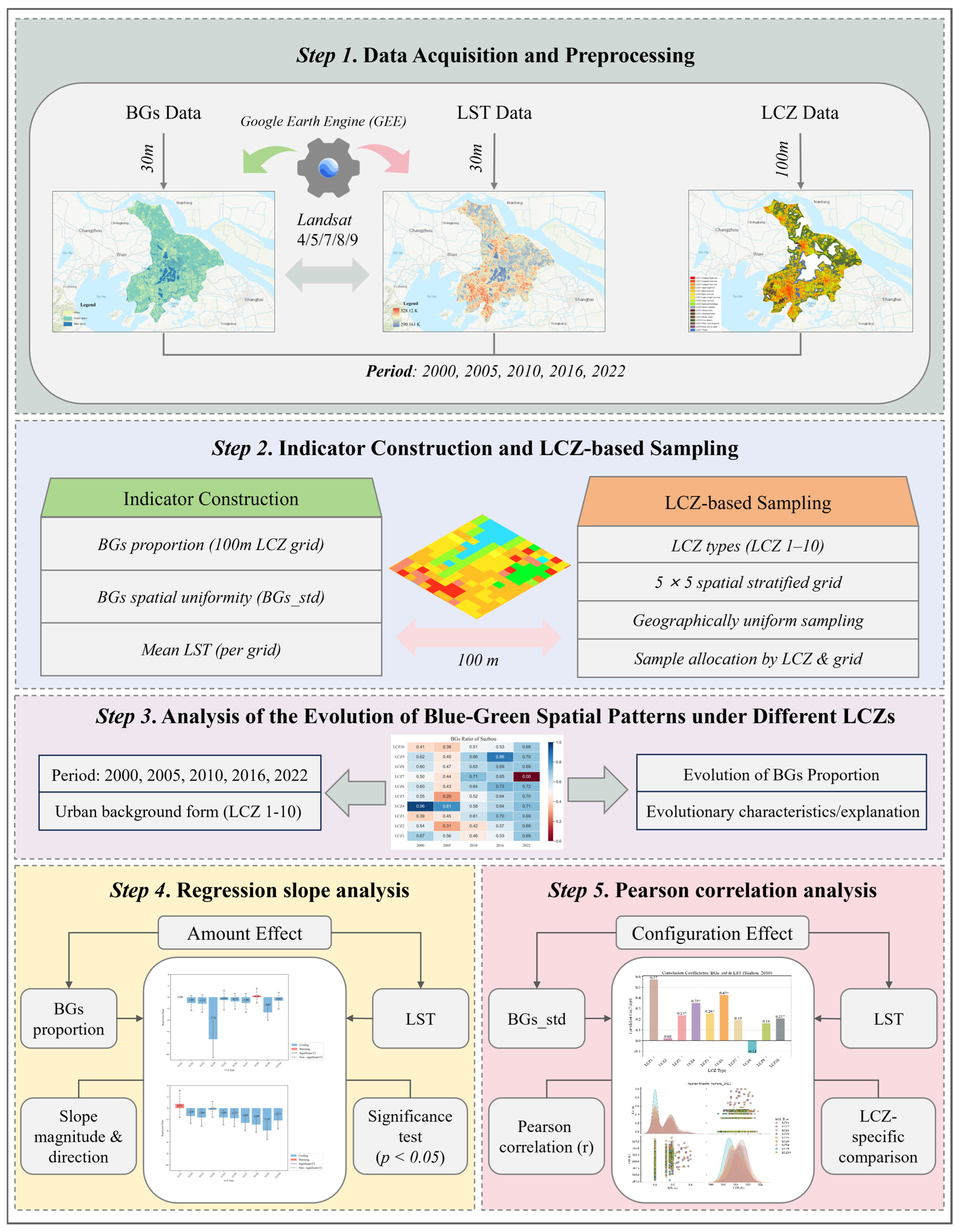
As shown in Figure 2, the overall research framework consists of five integrated components. Part I uses the GEE platform to acquire Landsat 4/5/7/8 series remote-sensing imagery for 2000, 2005, 2010, 2016, and 2022. This stage involves the extraction of BGs data and the retrieval of LST. Concurrently, 100 m resolution LCZ data were incorporated to provide the necessary urban morphological context for subsequent analysis. Part II focuses on indicator construction and LCZ-based sampling. At the 100 m LCZ (1–10) grid scale, key metrics were calculated, including BGs proportion, the standard deviation of BGs (BGs_std), and mean LST per grid. A 5 × 5 spatial stratification combined with a geographically uniform sampling method was employed to allocate samples representatively across different LCZ types and grid units. Part III analyzes the evolution of BGs patterns under different LCZ types. This involves a focused examination of the trends and characteristics of BGs proportion changes across five periods within each LCZ category. Part IV employs regression slope analysis to quantify the magnitude and direction of regression slopes for each LCZ type in each study year. Based on significance testing (p < 0.05), it examines the strength and direction of the association between BGs proportion on LST, thereby identifying amount-related cooling effects across distinct LCZ types. Part V employs Pearson correlation analysis to examine the relationship between the within-grid local dispersion of BGs (represented by BGs_std) and LST, as well as to compare how this BGs_std–LST relationship varies across different LCZ types.

2.3.1. LST Retrieval

This study employed the statistical mono-window (SMW) algorithm [37] on the GEE platform to systematically invert surface temperatures from Landsat series satellite imagery (including bands 4/5/7/8/9) for five representative years: 2000, 2005, 2010, 2016, and 2022.
L S T = A i T b ε + B i 1 ε + C i
where T b denotes the top-of-atmosphere brightness temperature of the thermal infrared band, and ε represents the surface emissivity of the corresponding band. The algorithm coefficients A i , B i and C i are empirical parameters derived from linear regression based on radiative transfer simulations conducted under ten different atmospheric water vapor conditions. By combining surface emissivity with these atmospheric parameters, the algorithm enables surface temperature to be estimated from a single thermal infrared band.

2.3.2. Regression Slope

To quantify the response of LST to changes in BGs proportion across different LCZ types, this study utilized a regression slope analysis framework. First, samples were collected according to the principle of geographic uniformity [41]. For each LCZ category, the study area was divided into a regular 5 × 5 spatial grid. This grid configuration was selected as a practical compromise between capturing intra-LCZ spatial heterogeneity and maintaining sufficient valid samples within each stratum for stable analysis. A coarser stratification would be less effective in representing spatial variability, whereas a finer stratification could lead to excessive fragmentation and insufficient samples in some subregions. The proportion of valid data points within each grid cell was calculated, and sample quantities were proportionally allocated to ensure a spatially uniform distribution, thereby mitigating biases arising from spatial clustering or sparsity. In most LCZ–year combinations, the final retained sample size reached 100, indicating that the geographically uniform sampling scheme achieved relatively balanced coverage across LCZ types and years (Table A1). Univariate linear regression models were established for each LCZ type, with BGs proportion within grid cells as the independent variable and the corresponding LST as the dependent variable. The analysis focused on the regression slope. First, the statistical significance of the relationship between BGs proportion and LST was assessed by examining whether the p-value of the slope coefficient was less than 0.05. If the relationship was statistically significant, further interpretation was based on the sign and absolute value of the slope: a negative slope indicated that higher BGs proportion was associated with a cooling effect, with a larger absolute value indicating a stronger cooling association; a positive slope indicated that higher BGs proportion was associated with warming. Finally, by comparing the absolute values of the slopes across all LCZ types, the LCZ types in which BGs proportion showed the strongest association with surface thermal conditions could be identified.

2.3.3. Within-Grid Local Dispersion Indicator of BGs (BGs_std)

To characterize the within-grid local dispersion of BGs, this study constructed an indicator denoted as BGs_std. At the 100 m LCZ grid scale, BGs_std was calculated as the standard deviation of 30 m BGs pixel values within each grid cell. A larger BGs_std indicates a higher degree of local dispersion of BGs within the grid, whereas a smaller value indicates a lower degree of local dispersion.
The BGs_std was calculated as follows:
B G s _ s t d = 1 N i = 1 N x i x ¯ 2
Here, x i represents the BGs value of a specific 30 m pixel within the grid (1 indicates presence of BGs, 0 indicates absence). Each x i corresponds to a single pixel value at 30 m resolution. x ¯ denotes the mean value of all 30 m pixel BGs within the 100 m grid, effectively representing the proportional coverage of BGs in that grid. BGs_std reflects the degree of local dispersion of BGs within a grid cell. A larger standard deviation indicates that BGs are distributed more unevenly among the 30 m pixels within the grid, whereas a smaller standard deviation suggests a less dispersed and more locally consistent BGs pattern.
Because BGs were coded as a binary variable in this study (BGs = 1, non-BGs = 0), BGs_std is mathematically related to BGs proportion within the same grid cell. If BGs proportion within a grid cell is denoted as p , then the standard deviation of the binary BGs distribution can be expressed as
B G s _ s t d = p 1 p
where p denotes the proportional coverage of BGs within the grid cell. Under this binary coding framework, BGs_std therefore reflects the degree of within-grid local dispersion between BGs and non-BGs at the 100 m LCZ-unit scale.
In this study, BGs_std was used as an indicator of the within-grid local dispersion of BGs. Compared with conventional landscape pattern metrics such as patch size, fragmentation, clustering, or connectivity, BGs_std does not aim to fully represent all aspects of landscape configuration. Instead, it captures one specific dimension of spatial organization, namely the degree of local dispersion of BGs within a relatively homogeneous LCZ unit. This indicator is particularly suitable for comparative analysis across years and LCZ types under a consistent grid-based framework.

2.3.4. Pearson Correlation Coefficient

To investigate the relationship between the within-grid local dispersion of BGs and LST, this study employed Pearson correlation analysis. Consistent with the sampling method described above, geographically uniform sampling was used to ensure sufficient and representative samples across different LCZ types for the subsequent analysis.
Subsequently, the Pearson correlation coefficient r was employed to assess the linear relationship between BGs_std and the corresponding LST values across different LCZ types. The calculation formula is as follows:
r = i = 1 n X i X ¯ Y i Y ¯ i = 1 n ( X i X ¯ ) 2 i = 1 n ( Y i Y ¯ ) 2
where X i and Y i represent the BGs_std and LST values for the i-th sample, respectively, and X ¯ and Y ¯ denote their respective means. n is the number of samples. The correlation coefficient r ranges from −1 to 1. A positive value indicates positive correlation, a negative value indicates negative correlation, and a larger absolute value indicates stronger correlation.

3. Results and Analysis

3.1. LST Retrieval Using GEE

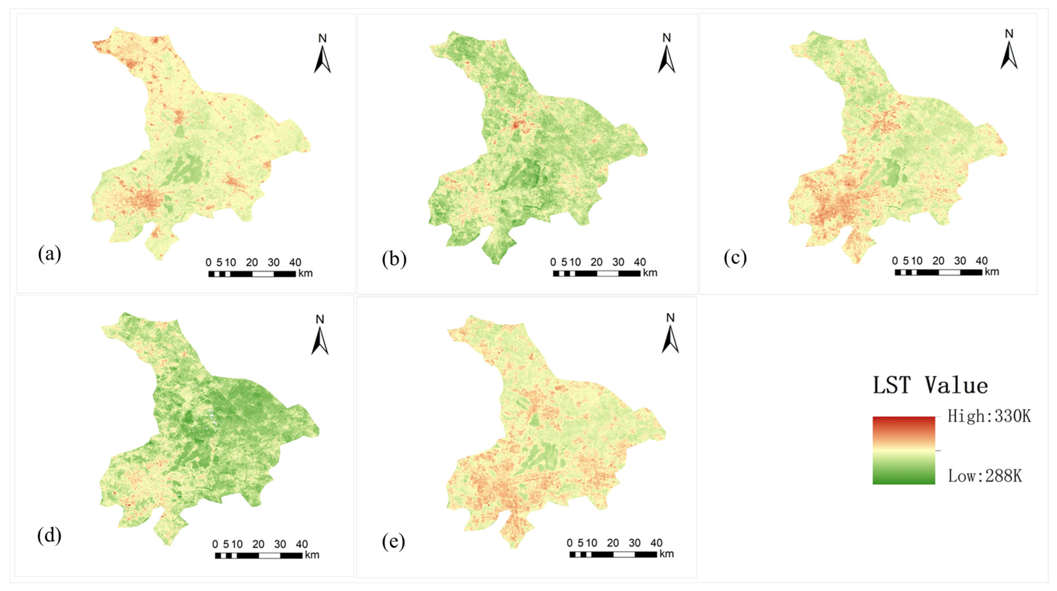
Figure 3 shows the spatial distribution of LST in Suzhou for five representative years: 2000, 2005, 2010, 2016, and 2022. Overall, the study area exhibited a clear stage-based pattern of LST from 2000 to 2022. In 2000, LST was predominantly low to moderate, with limited spatial variation and only scattered high-temperature patches. By 2005, high-temperature zones expanded noticeably. Areas previously characterized by moderate-to-high temperatures developed into zones with different degrees of heat intensity. This shift may have been related to Suzhou’s rapid urban development during this period, which was accompanied by increasing impervious surfaces and intensified localized warming. In 2010, overall LST was lower than in 2005, as reflected by the expansion of low-to-moderate temperature zones and a partial reduction in high-temperature areas. LST further declined in 2016, with low-temperature areas becoming more widespread and the overall thermal pattern becoming more moderated. By 2022, LST had rebounded, with medium-to-high temperature zones re-expanding as concentrated patches in certain areas. Overall, the study area exhibited a fluctuating thermal pattern over the study period, characterized by a rise, a decline, and then a subsequent rise in LST. These temporal changes were broadly consistent with the different stages of urban development in Suzhou.

3.2. Analysis of the Evolution of BGs Patterns Under Different LCZ Types

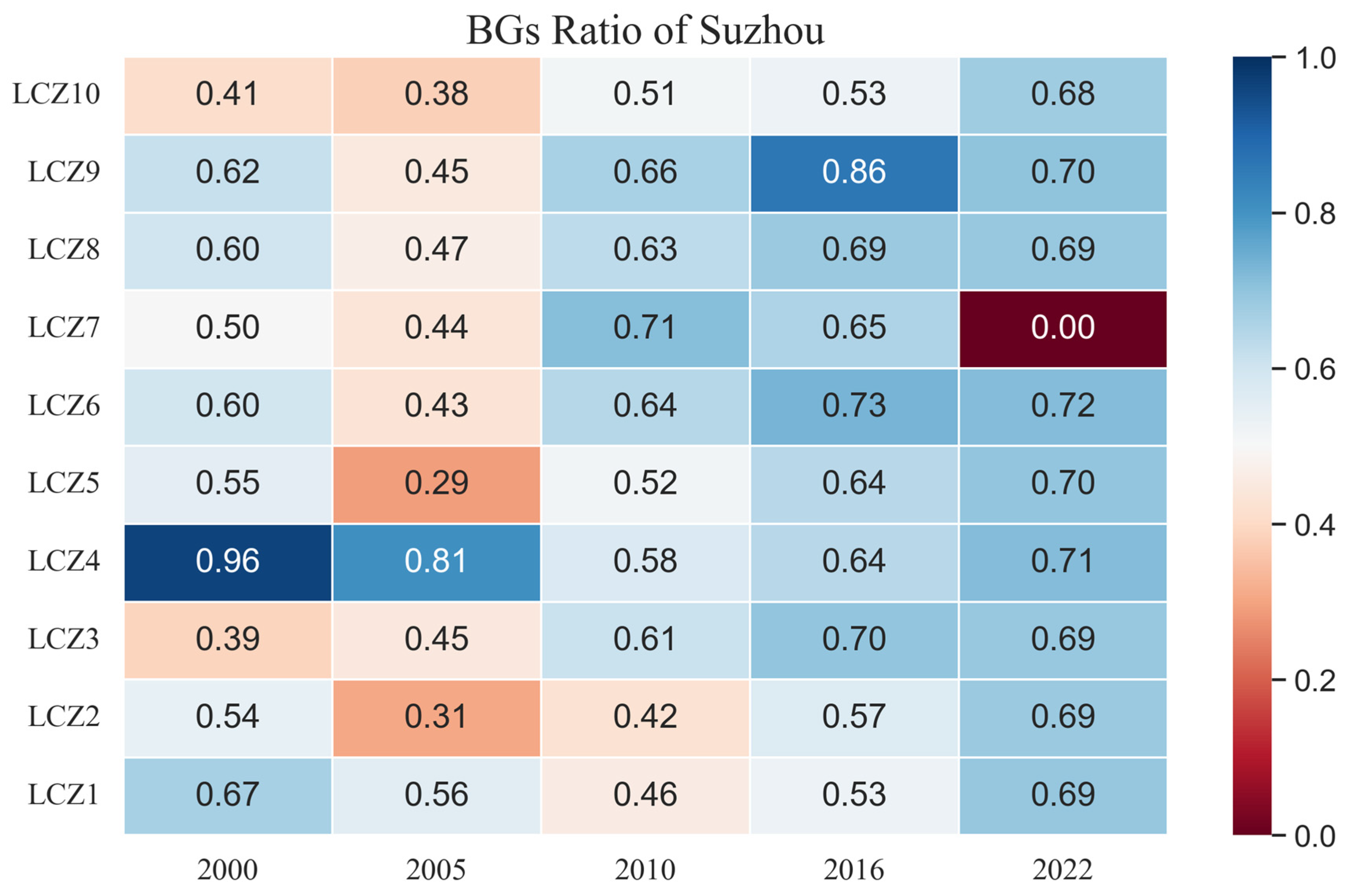
As shown in Figure 4, BGs proportion across most LCZ types exhibited a general upward trend from 2000 to 2022. Among them, LCZ 3 (Compact low-rise) and LCZ 10 (Heavy industry) showed the largest increases in BGs proportion. Their peak values were 0.30 and 0.27, occurring in 2016 and 2022, respectively. However, LCZ 4 (Open high-rise) and LCZ 7 (Lightweight low-rise) exhibited clear declining trends. This indicated that BGs evolved differently among LCZ types. This pattern suggested that BGs in some high-intensity development areas or functionally designated lands were maintained or adjusted in different ways over time. Over the 22-year period, BGs proportion in LCZ 4 and LCZ 7 decreased by 0.25 and 0.50, respectively. LCZ 4 reached a low value of 0.58 in 2010, and LCZ 7 fell to nearly zero by 2022. This suggested that BGs in these urban forms may have been substantially reduced during rapid urban development or land-use restructuring.
Stage-based analysis suggested that 2005 may have represented an important turning point, as BGs proportion decreased in all categories except LCZ 1 (Compact high-rise). This pattern indicated that the early stage of Suzhou’s urban expansion was accompanied by a reduction in internal BGs and the conversion of natural or semi-natural surfaces.
A comparative analysis of LCZ types showed that in 2000, the highest BGs proportion was 0.96 in LCZ 4, whereas the lowest values were 0.39 in LCZ 3 and 0.41 in LCZ 10. The other LCZ types generally ranged from 0.5 to 0.6. This indicated substantial differences in BGs distribution among LCZ types at the beginning of the study period. By 2022, excluding LCZ 7, all other LCZ types had converged toward a BGs proportion of around 0.7. This suggested a tendency toward convergence in BGs proportion across most LCZ types during urban development. Although LCZ 4 showed a decreasing trend, it still maintained a relatively high BGs proportion. This suggested that open high-rise zones tended to retain comparatively high BGs levels over time.

3.3. Analysis of LST Effects from BGs Proportion Changes Across LCZ Types via Regression Slope

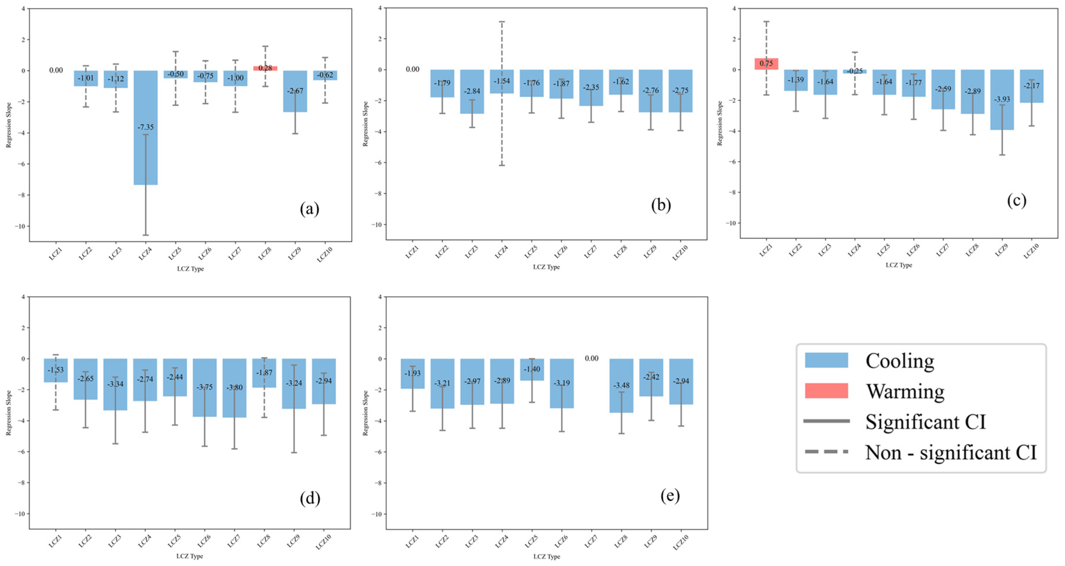
Figure 5 shows the regression slopes and significance levels for the relationship between BGs proportion and LST across different LCZ types in 2000, 2005, 2010, 2016, and 2022. Predominantly negative regression slopes were observed across most years and LCZ types, indicating that higher BGs proportion was generally associated with a cooling effect.
The magnitude and statistical significance of this cooling association varied over time (Table A2). In 2005, 2016, and 2022, regression slopes for most LCZ types were statistically significant, indicating relatively strong cooling associations between BGs proportion and LST. In contrast, fewer statistically significant relationships were observed in 2000 and 2010. One possible explanation was that the cooling association of BGs varied across different stages of urban development. In earlier or more rapidly developing stages, BGs may have been smaller, more fragmented, or less ecologically mature, which may have reduced the strength of their observed cooling associations. By contrast, during relatively stable development or ecological restoration stages, more connected or ecologically mature BGs may have been more strongly associated with lower LST.
Comparative analysis showed that LCZ 2 (Compact mid-rise), LCZ 3 (Compact low-rise), LCZ 6 (Open low-rise), LCZ 9 (Scattered buildings), and LCZ 10 (Heavy industry) exhibited markedly negative regression slopes over multiple years. This suggested that cooling effects were observed in all of these LCZ types. The strength of this cooling effect differed among LCZ types, implying that the BGs–LST relationship may vary under different urban morphological contexts.
It should also be noted that the regression slopes for LCZ 1 (Compact high-rise) and LCZ 8 (Large low-rise) were positive in 2000 and 2010. This indicated that, in these specific cases, higher BGs proportion was associated with higher LST. However, this pattern occurred only in some years and LCZ types.

3.4. Correlation Analysis of Within-Grid Local Dispersion of BGs and LST Across Different LCZ Types

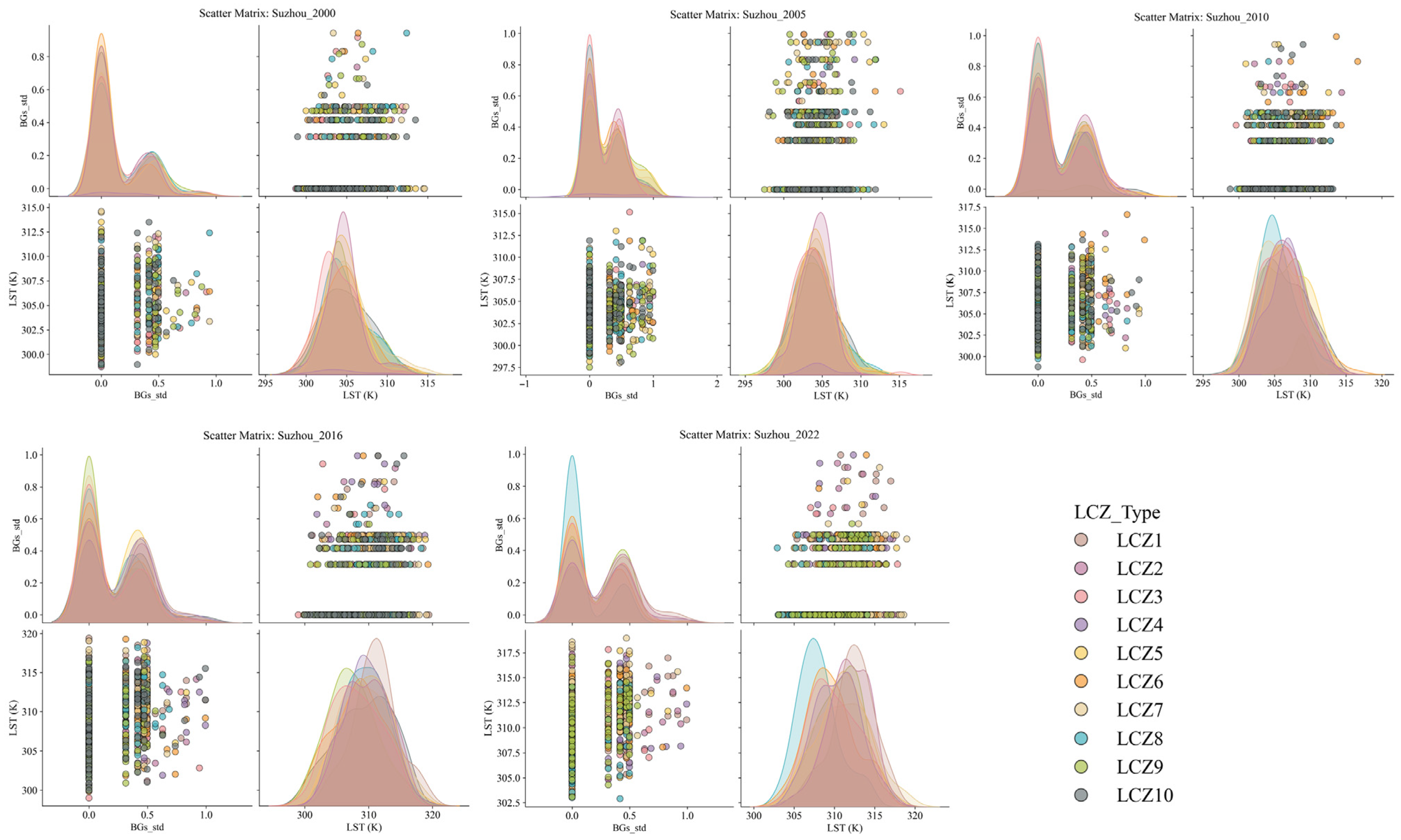
Figure 6 shows the scatter matrix of BGs_std and LST in Suzhou for five representative years, classified by LCZ types. The probability density distribution of BGs_std showed that values in different years were mainly concentrated within a relatively low range and exhibited distinct unimodal or weakly bimodal characteristics. This suggested that the within-grid local dispersion of BGs was relatively low in most parts of the study area. Although BGs_std distributions differed somewhat among LCZ types, their overall ranges overlapped substantially. This indicated that no clear separation in within-grid local dispersion was observed among LCZ types at the aggregate level. The probability density distribution of LST over the study period showed greater interannual variability. Over time, the range of the LST distribution gradually expanded. The frequency of both high- and low-temperature extremes also increased. This indicated that the overall LST distribution became more dispersed across the study area. Meanwhile, differences in LST among LCZ types became increasingly evident in recent years. This suggested that thermal contrasts among different urban morphological units intensified with urbanization.
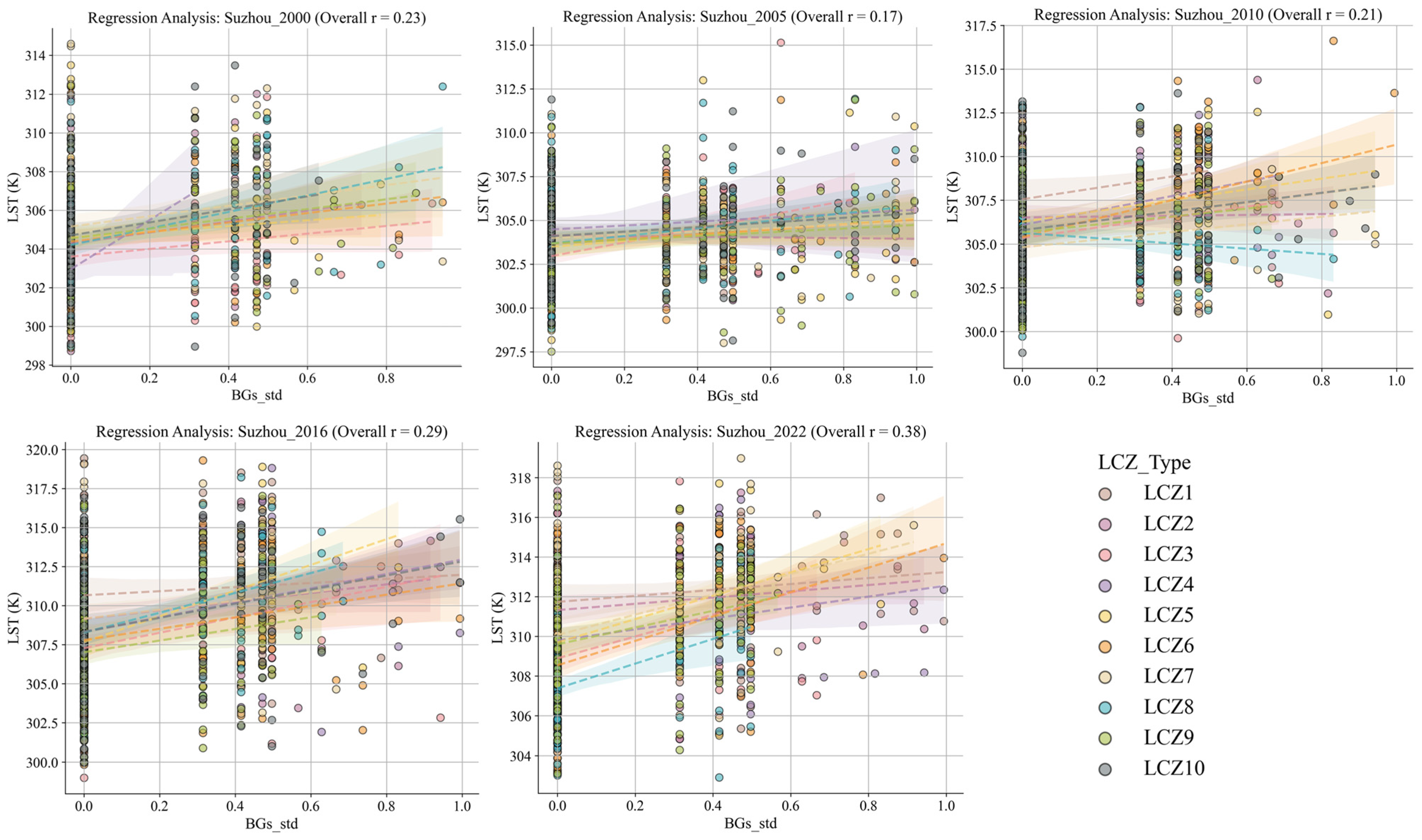
Based on the above results, the statistical relationship between BGs_std and LST was further examined using scatter plots and regression analysis. As shown in Figure 7, a positive correlation between BGs_std and LST was observed in all five representative years. In other words, higher BGs_std values were generally associated with higher LST. This suggested that greater within-grid local dispersion of BGs tended to coincide with warmer surface conditions. Conversely, lower within-grid local dispersion of BGs was associated with lower LST at the grid scale. The corresponding overall correlation coefficients (r) were 0.23 in 2000, 0.17 in 2005, 0.21 in 2010, 0.29 in 2016, and 0.38 in 2022. This suggested that the positive correlation between the within-grid local dispersion of BGs and LST persisted throughout the study period, although the strength of the relationship varied over time.
Over time, the correlation between BGs_std and LST generally strengthened. The overall correlation coefficients in 2016 and 2022 were notably higher than those in the preceding years. This suggested that, in the later part of the observation period, the relationship between the within-grid local dispersion of BGs and LST became more evident. In contrast, correlations in 2000 and 2005 were relatively weak, with greater data dispersion and less differentiation among the regression trend lines across different LCZ types.
Analysis of the regression results across different LCZ types revealed predominantly positive fitted slopes, although their magnitude and dispersion varied considerably. This implied that the relationship between BGs_std and LST was not uniform across different urban morphological units. Some LCZ types maintained relatively stable positive regression trends throughout the study period, whereas others shifted from weak or negligible correlations in earlier stages to clearer regression relationships in later years. This further suggested that the statistical relationship between the within-grid local dispersion of BGs and LST exhibited substantial heterogeneity across both temporal and spatial dimensions.
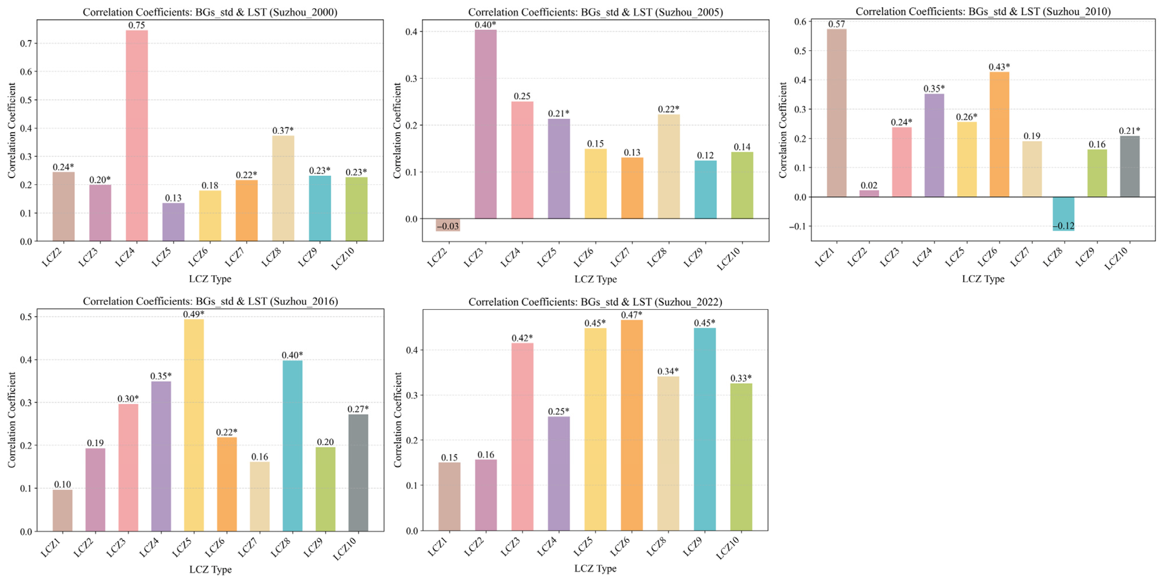
Based on the scatter distribution characteristics and overall regression trends described above, the statistical relationship between BGs_std and LST at the grid-unit scale was further quantified using Pearson correlation coefficients (Table A3). As shown in Figure 8, a relatively strong positive linear correlation was observed between BGs_std and LST in LCZ 4 in 2000, although it was not statistically significant, likely because of the limited sample size of LCZ 4 units in that year. In the remaining four years (2005, 2010, 2016, and 2022), the LCZ types exhibiting the strongest positive linear correlations were LCZ 3, LCZ 1, LCZ 5 (Open mid-rise), and LCZ 6, respectively. This highlighted differences in the strength of the BGs_std–LST relationship across LCZ types. These results suggested that the association between the within-grid local dispersion of BGs and LST differed among urban morphological contexts. In some LCZ types, this relationship appeared relatively stronger, whereas in others it was weaker or less stable. This pattern indicated that BGs_std–LST relationships were not uniform across LCZ types.
Notably, weak negative linear correlations were observed in LCZ 2 (2010) and LCZ 8 (2016). These exceptions suggested that the BGs_std–LST relationship was not fully consistent across all LCZ types and years. Such fluctuations may have been related to differences in developmental context, scale effects, or sample conditions, although these factors were not directly examined in the present analysis. However, such weak negative correlations were limited to a small number of LCZ types and years. They did not alter the broader pattern observed in this study, namely that lower within-grid local dispersion of BGs was generally associated with lower LST over the study period.

4. Discussion

4.1. Comparison with Existing Research

Most previous studies conducted at regional or city scales have reported that higher BGs coverage is generally associated with lower LST, and this broad pattern has been observed across many urban and climatic contexts [25,42]. The results of the present study are broadly consistent with this finding. Across most LCZ types and study years, higher BGs proportion was associated with lower LST. This suggested that BGs remained closely related to surface thermal patterns in Suzhou.
At the same time, the present study suggests that BGs proportion alone does not fully account for variation in LST across different LCZ types. Even where BGs proportions were relatively similar, LST levels still differed among LCZ-defined urban morphological units. This pattern suggests that BGs–LST relationships should be interpreted together with differences in urban form. In this sense, the contribution of this study lies not in proposing a new methodological framework but in applying an LCZ-based comparative perspective to show that BGs–LST relationships vary across urban morphological contexts.
The present findings are also broadly consistent with previous studies that have emphasized the relevance of BGs spatial pattern to urban thermal conditions [43,44]. In this study, BGs_std was used to characterize the within-grid local dispersion of BGs within 100 m LCZ units. The results showed that higher BGs_std values were generally associated with higher LST. This suggested that the spatial organization of BGs within LCZ units may be relevant to LST patterns. Compared with previous studies based on patch metrics or city-wide summary indicators, the LCZ-based framework adopted here further suggested that the strength of this relationship differed across urban morphological units.
Another point worth noting is that relationships observed at smaller spatial scales were not always reproduced at the LCZ-unit scale. In some LCZ types and years, lower BGs_std values were associated with lower LST. However, this pattern was not universal when LST was evaluated as an average condition over the entire LCZ unit. This suggested that the BGs–LST relationship may vary with analytical scale and urban morphological context. From this perspective, the present study provided empirical evidence that scale and unit definition were important. This helps explain why conclusions from previous BGs-related studies were not always directly comparable.
Overall, the present study provided an integrative and exploratory empirical perspective on BGs–LST relationships under different urban morphological contexts. Its main value lay in showing, within a unified LCZ-based framework, that BGs proportion and within-grid local dispersion were associated with LST in different ways. These differences were observed across urban morphological units and representative stages of Suzhou’s development from 2000 to 2022. These findings may provide context-sensitive reference information for urban ecological planning. However, they should be interpreted cautiously because the present analysis was based on LST and statistical associations rather than on direct evidence of thermal comfort or causal mechanisms.

4.2. Planning Implications Based on BGs–LST Relationships

The results of this study suggested that BGs–LST relationships should be interpreted with attention to urban morphological context. Under the LCZ framework, the statistical associations between BGs characteristics and LST were not uniform across urban form types. This indicated that the thermal relevance of BGs may vary among different built environments.
In particular, the findings implied that variation in BGs proportion and within-unit BGs arrangement may have been more strongly reflected in LST in some LCZ types than in others. By contrast, in LCZ types where these associations were weaker or less consistent, the observed LST patterns may also have reflected the influence of additional local factors beyond BGs characteristics alone. This indicated that the relationship between BGs and surface thermal conditions should not be interpreted as spatially uniform across all urban settings.
The results also suggest that BGs–LST relationships were not adequately explained by BGs area alone. Within the LCZ-unit framework adopted in this study, the within-unit spatial organization of BGs was also statistically associated with LST in several cases. This means that, when interpreting BGs-related thermal patterns, attention should be given not only to the amounts of BGs present, but also to how BGs are distributed across different urban morphological contexts.
From this perspective, the LCZ framework provides a useful basis for comparing where BGs–LST associations are relatively stronger or weaker across different urban form types. However, because the present analysis was based on LST and statistical associations, these findings should be understood as context-specific interpretive evidence. They should not be taken as direct prescriptive guidance for planning practice.

4.3. Limitations of This Study

This study should be regarded as an exploratory analysis. The empirical framework was limited to univariate linear regression and Pearson correlation. These methods were useful for identifying general linear association patterns, but they could not fully capture more complex relationships. Future research could employ nonlinear or multivariable approaches to provide a more comprehensive understanding of BGs–LST relationships.
Another limitation is that the study used only five representative years between 2000 and 2022. Although these temporal nodes were selected to reflect major stages of Suzhou’s development, they cannot fully represent continuous year-to-year dynamics. Therefore, the long-term conclusions of this study should be interpreted as stage-based comparisons. Future studies could include denser annual observations to further examine temporal stability.
In addition, BGs_std was used as a measure of the within-grid local dispersion of BGs. Because BGs_std was calculated from binary 0/1 BGs values within each 100 m grid cell, it was mathematically related to BGs proportion under the present analytical framework. Therefore, its interpretation in this study is limited to within-grid local dispersion at the LCZ-unit scale. This metric is useful under the unified 100 m LCZ framework, but it cannot fully represent more detailed landscape pattern characteristics. Moreover, the 100 m spatial scale used in this study is not ideal for applying finer landscape metrics in a robust and comparable way. Future research could integrate higher-resolution data with more specific landscape pattern indicators.
Furthermore, the BGs extraction procedure applied consistent NDVI and MNDWI thresholds across different years and Landsat sensors to ensure interannual comparability. Although this strategy improved the consistency of the long-term analysis, it may also introduce uncertainty. Spectral responses can vary across sensors, years, and surface conditions, which could affect the results. Therefore, some uncertainty may remain in the extracted BGs maps. This is particularly true when comparing results across a long time span.
Finally, the thermal indicator used in this study was remotely sensed LST. Although LST is widely used to describe surface thermal conditions, it is not the same as near-surface air temperature. It cannot directly represent human thermal comfort, especially in densely built environments. Therefore, the findings of this study should be interpreted specifically in relation to surface thermal patterns. Future studies could incorporate air temperature, humidity, wind speed, and thermal comfort indices such as the Universal Thermal Climate Index (UTCI) for a more comprehensive evaluation.

5. Conclusions

This study used remote-sensing data from five representative years (2000, 2005, 2010, 2016, and 2022), together with the LCZ classification system, to examine BGs–LST associations in the built-up area of Suzhou. Based on this, four aspects were selected for synthesis: the evolution of LST, changes in BGs, BGs proportion across different LCZ types, and the within-grid local dispersion of BGs.
First, based on multi-period remote-sensing images from 2000, 2005, 2010, 2016, and 2022, this study examined the spatiotemporal evolution of surface thermal patterns in Suzhou’s built-up area using LST retrieval. The results showed that LST in Suzhou exhibited a “rise–decline–rise” pattern during the study period. The extent and intensity of high-temperature zones changed in distinct stages, which were broadly consistent with different phases of urban development. In addition, this study quantitatively analyzed the spatiotemporal changes in BGs proportions across different LCZ types. The findings show that both the direction and magnitude of changes in BGs proportions differed across LCZ types from 2000 to 2022. Most LCZ types exhibited an overall upward trend, with LCZ 3 and LCZ 10 showing the largest increases, peaking in 2016 and 2022, respectively. LCZ 4 and LCZ 7 exhibited significant decreases, reaching their lowest levels in 2010 and 2022, respectively. This suggests that BGs in these zones may have been substantially reduced due to urban expansion or land-use restructuring. In 2005, all LCZ types except LCZ 1 showed varying degrees of decline in BGs proportion, suggesting that BGs changes differed across built-up morphologies.
Regression slope analysis was used to examine the direction and magnitude of the relationship between BGs proportion and LST. Across the five study years, most LCZ types exhibited negative regression slopes, suggesting that higher BGs proportion was generally associated with a cooling effect. LCZ 2, LCZ 3, LCZ 6, LCZ 9, and LCZ 10 showed significant negative regression slopes in multiple years, indicating a relatively stable cooling effect. However, positive relationships were also observed in 2000 and 2010 for some LCZ types, such as LCZ 1 and LCZ 8, where higher BGs proportions were associated with higher LST. This may indicate that, in some earlier or rapidly developing stages, the association between BGs proportions and LST was weaker or more variable under certain built-form conditions. Pearson correlation analysis further showed that BGs_std, representing the within-grid local dispersion of BGs, was associated with LST. Across the study years, BGs_std was positively associated with LST, and this relationship strengthened over time. This suggests that, at the LCZ-unit scale, greater within-grid local dispersion of BGs was generally associated with higher LST. In other words, the strength of this relationship differed among LCZ types. The relationship appeared relatively stronger in LCZ types such as LCZ 1, LCZ 3, LCZ 5, and LCZ 6. This further suggests that BGs–LST associations varied with urban form.

Author Contributions

Conceptualization, C.Z. and Y.Q.; methodology, Y.L., H.Y. and Y.Q.; software, Y.L., H.Y. and Y.Q.; validation, Y.L., C.Z. and Y.Q.; formal analysis, Y.L. and Y.Q.; investigation, Y.L. and Y.Q.; resources, C.Z.; data curation, Y.L., H.Y. and Y.Q.; writing—original draft preparation, Y.L. and Y.Q.; writing—review and editing, Y.L. and Y.Q. and C.Z.; visualization, Y.L. and Y.Q.; supervision, C.Z.; project administration, C.Z.; funding acquisition, C.Z. All authors have read and agreed to the published version of the manuscript.

Funding

This work was supported by the National Natural Science Foundation of China (grant number 42371425).

Data Availability Statement

LCZ classification data were sourced from the publicly available dataset, “Annual Local Climate Zones at 100-Meter Resolution for China’s Major Cities, 2000–2022” (Access URL: https://doi.org/10.5281/zenodo.14614256). BGs data were derived following the processing workflow described by Qi, Y.; Zhang, C.; Pei, S.; Yu, H.; Hu, Y. Spatiotemporal evolution of the cooling effect of blue-green space in different LCZs: A comparative study of Wuhan and Shanghai (2000–2022). Urban Climate 2025, 64, 102723 (https://doi.org/10.1016/j.uclim.2025.102723) [15]. The source code used for LST retrieval is publicly available from Google Earth Engine at: https://code.earthengine.google.com/?accept_repo=users/sofiaermida/landsat_smw_lst (accessed on 26 October 2025). The BGs and LCZ datasets used in this study are publicly available at GitHub: https://github.com/Dan54613/suzhou-bgs-lcz-data (accessed on 26 October 2025).

Conflicts of Interest

The authors declare no conflicts of interest.

Abbreviations

The following abbreviations are used in this manuscript:
BGsBlue–green spaces
LSTLand Surface Temperature
LCZLocal Climate Zone
stdstandard deviation
GEEGoogle Earth Engine
UTCIUniversal Thermal Climate Index

Appendix A

This appendix provides supplementary statistical information supporting the main analyses. Table A1 summarizes the number of retained samples for each year and LCZ type after geographically uniform sampling. Table A2 reports the regression slope analysis results between BGs proportion and LST across years and LCZ types, including slope estimates, p-values, and 95% confidence intervals. Table A3 presents the Pearson correlation results between BGs_std and LST for different years and LCZ types. Together, these tables provide detailed statistical evidence for the BGs–LST relationships discussed in the main text.
Table A1. Number of retained samples for each year and LCZ type after geographically uniform sampling.
LCZ Type20002005201020162022
LCZ 11122100100
LCZ 2100100100100100
LCZ 3100100100100100
LCZ 4253788100100
LCZ 5100100100100100
LCZ 6100100100100100
LCZ 71001001001000
LCZ 8100100100100100
LCZ 9100100100100100
LCZ 10100100100100100
Table A2. Summary of regression slope analysis results between BGs proportion and LST across years and LCZ types.
YearLCZ TypeSlopep-Value95% CI
2000LCZ 10.000NA *NA
LCZ 2−1.0100.133[−2.332, 0.313]
LCZ 3−1.1170.152[−2.653, 0.419]
LCZ 4−7.3500.005[−10.582, −4.118]
LCZ 5−0.4970.569[−2.225, 1.230]
LCZ 6−0.7480.284[−2.127, 0.631]
LCZ 7−0.9990.239[−2.671, 0.674]
LCZ 80.2800.668[−1.011, 1.571]
LCZ 9−2.6700.000[−4.056, −1.284]
LCZ 10−0.6170.406[−2.083, 0.849]
2005LCZ 10.000NANA
LCZ 2−1.7910.001[−2.822, −0.759]
LCZ 3−2.8440.001[−3.735, −1.953]
LCZ 4−1.5400.433[−6.185, 3.104]
LCZ 5−1.7600.001[−2.798, −0.723]
LCZ 6−1.8750.004[−3.134, −0.615]
LCZ 7−2.3460.000[−3.400, −1.292]
LCZ 8−1.6180.004[−2.709, −0.526]
LCZ 9−2.7560.000[−3.880, −1.631]
LCZ 10−2.7530.001[−3.931, −1.575]
2010LCZ 10.7460.503[−1.645, 3.136]
LCZ 2−1.3870.041[−2.175, −0.060]
LCZ 3−1.6350.038[−3.175, −0.095]
LCZ 4−0.2470.724[−1.632, 1.138]
LCZ 5−1.6410.014[−2.942, −0.341]
LCZ 6−1.7670.019[−3.241, −0.294]
LCZ 7−2.5870.001[−3.963, −1.212]
LCZ 8−2.8890.000[−4.240, −1.538]
LCZ 9−3.9330.004[−5.565, −2.300]
LCZ 10−2.1670.005[−3.672, −0.662]
2016LCZ 1−1.5270.092[−3.306, 0.253]
LCZ 2−2.6490.004[−4.452, −0.845]
LCZ 3−3.3430.003[−5.496, −1.190]
LCZ 4−2.7390.008[−4.744, −0.734]
LCZ 5−2.4360.010[−4.283, −0.589]
LCZ 6−3.7510.001[−5.657, −1.845]
LCZ 7−3.8010.000[−5.827, −1.776]
LCZ 8−1.8720.056[−3.792, 0.047]
LCZ 9−3.2380.025[−6.062, −0.414]
LCZ 10−2.9410.004[−4.946, −0.937]
2022LCZ 1−1.9320.010[−3.384, −0.481]
LCZ 2−3.2101.666[−4.616, −1.804]
LCZ 3−2.9720.000[−4.480, −1.465]
LCZ 4−2.8920.000[−4.478, −1.306]
LCZ 5−1.4050.050[−2.807, −0.003]
LCZ 6−3.1940.000[−4.685, −1.702]
LCZ 70.000NANA
LCZ 8−3.4810.000[−4.823, −2.140]
LCZ 9−2.4250.002[−3.973, −0.876]
LCZ 10−2.9440.001[−4.336, −1.552]
* NA indicates that the data is unavailable due to an insufficient sample size.
Table A3. Summary of Pearson correlation analysis results between BGs_std and LST across years and LCZ types.
YearLCZ TypeCorrelationp-Value
2000LCZ 20.2440.015
LCZ 30.1990.047
LCZ 40.7450.148
LCZ 50.1350.182
LCZ 60.1790.075
LCZ 70.2150.031
LCZ 80.3730.001
LCZ 90.2310.021
LCZ 100.2260.025
2005LCZ 2−0.0270.787
LCZ 30.4030.002
LCZ 40.2500.588
LCZ 50.2130.034
LCZ 60.1490.139
LCZ 70.1300.196
LCZ 80.2230.026
LCZ 90.1240.221
LCZ 100.1420.158
2010LCZ 10.5730.051
LCZ 20.0220.829
LCZ 30.2370.018
LCZ 40.3520.000
LCZ 50.2560.011
LCZ 60.4270.001
LCZ 70.1900.059
LCZ 8−0.1170.250
LCZ 90.1620.107
LCZ 100.2080.038
2016LCZ 10.0970.341
LCZ 20.1930.057
LCZ 30.2960.003
LCZ 40.3490.001
LCZ 50.4930.000
LCZ 60.2180.030
LCZ 70.1610.110
LCZ 80.3980.000
LCZ 90.1950.051
LCZ 100.2720.006
2022LCZ 10.1500.137
LCZ 20.1560.121
LCZ 30.4150.002
LCZ 40.2520.011
LCZ 50.4480.000
LCZ 60.4660.001
LCZ 70.3410.001
LCZ 80.4490.000
LCZ 90.3260.001
LCZ 100.1500.137

References

  1. Grimmond, S. Urbanization and global environmental change: Local effects of urban warming. Geogr. J. 2007, 173, 83–88. [Google Scholar] [CrossRef] [Scilit]
  2. Santamouris, M. Analyzing the heat island magnitude and characteristics in one hundred Asian and Australian cities and regions. Sci. Total Environ. 2015, 512, 582–598. [Google Scholar] [CrossRef] [Scilit] [PubMed]
  3. Santamouris, M.; Cartalis, C.; Synnefa, A.; Kolokotsa, D. On the impact of urban heat island and global warming on the power demand and electricity consumption of buildings—A review. Energy Build. 2015, 98, 119–124. [Google Scholar] [CrossRef] [Scilit]
  4. Harlan, S.L.; Ruddell, D.M. Climate change and health in cities: Impacts of heat and air pollution and potential co-benefits from mitigation and adaptation. Curr. Opin. Environ. Sustain. 2011, 3, 126–134. [Google Scholar] [CrossRef] [Scilit]
  5. Zhou, D.; Xiao, J.; Bonafoni, S.; Berger, C.; Deilami, K.; Zhou, Y.; Frolking, S.; Yao, R.; Qiao, Z.; Sobrino, J.A. Satellite remote sensing of surface urban heat islands: Progress, challenges, and perspectives. Remote Sens. 2018, 11, 48. [Google Scholar] [CrossRef] [Scilit]
  6. Voogt, J.A.; Oke, T.R. Thermal remote sensing of urban climates. Remote Sens. Environ. 2003, 86, 370–384. [Google Scholar] [CrossRef] [Scilit]
  7. Fernandes, R.; Nascimento, V.; Freitas, M.; Ometto, J. Local climate zones to Identify Surface Urban Heat Islands: A systematic review. Remote Sens. 2023, 15, 884. [Google Scholar] [CrossRef] [Scilit]
  8. Feyisa, G.L.; Dons, K.; Meilby, H. Efficiency of parks in mitigating urban heat island effect: An example from Addis Ababa. Landsc. Urban Plan. 2014, 123, 87–95. [Google Scholar] [CrossRef] [Scilit]
  9. Bowler, D.E.; Buyung-Ali, L.; Knight, T.M.; Pullin, A.S. Urban greening to cool towns and cities: A systematic review of the empirical evidence. Landsc. Urban Plan. 2010, 97, 147–155. [Google Scholar] [CrossRef] [Scilit]
  10. Lin, P.; Lau, S.S.Y.; Qin, H.; Gou, Z. Effects of urban planning indicators on urban heat island: A case study of pocket parks in high-rise high-density environment. Landsc. Urban Plan. 2017, 168, 48–60. [Google Scholar] [CrossRef] [Scilit]
  11. Sun, R.; Chen, L. How can urban water bodies be designed for climate adaptation? Landsc. Urban Plan. 2012, 105, 27–33. [Google Scholar] [CrossRef] [Scilit]
  12. Qiu, X.; Kil, S.-H.; Jo, H.-K.; Park, C.; Song, W.; Choi, Y.E. Cooling effect of urban blue and green spaces: A case study of Changsha, China. Int. J. Environ. Res. Public Health 2023, 20, 2613. [Google Scholar] [CrossRef] [Scilit] [PubMed]
  13. Chen, A.; Yao, X.A.; Sun, R.; Chen, L. Effect of urban green patterns on surface urban cool islands and its seasonal variations. Urban For. Urban Green. 2014, 13, 646–654. [Google Scholar] [CrossRef] [Scilit]
  14. Guo, L.; Liu, R.; Men, C.; Wang, Q.; Miao, Y.; Zhang, Y. Quantifying and simulating landscape composition and pattern impacts on land surface temperature: A decadal study of the rapidly urbanizing city of Beijing, China. Sci. Total Environ. 2019, 654, 430–440. [Google Scholar] [CrossRef] [Scilit]
  15. Qi, Y.; Zhang, C.; Pei, S.; Yu, H.; Hu, Y. Spatiotemporal evolution of the cooling effect of blue-green space in different LCZs: A comparative study of Wuhan and Shanghai (2000−2022). Urban Clim. 2025, 64, 102723. [Google Scholar] [CrossRef] [Scilit]
  16. Yu, Z.; Yang, G.; Zuo, S.; Jørgensen, G.; Koga, M.; Vejre, H. Critical review on the cooling effect of urban blue-green space: A threshold-size perspective. Urban For. Urban Green. 2020, 49, 126630. [Google Scholar] [CrossRef] [Scilit]
  17. Marquez-Torres, A.; Kumar, S.; Aznarez, C.; Jenerette, G.D. Assessing the cooling potential of green and blue infrastructure from twelve US cities with contrasting climate conditions. Urban For. Urban Green. 2025, 104, 128660. [Google Scholar] [CrossRef] [Scilit]
  18. Yu, H.; Yu, L.; Zhang, C.; Qi, Y. How does urbanization process affect urban heat island effect? Interpretation of 31 cities in China based on local climate zones. Environ. Res. Lett. 2025, 20, 114013. [Google Scholar] [CrossRef] [Scilit]
  19. Stewart, I.D.; Oke, T.R. Local climate zones for urban temperature studies. Bull. Am. Meteorol. Soc. 2012, 93, 1879–1900. [Google Scholar] [CrossRef] [Scilit]
  20. Bechtel, B.; Alexander, P.J.; Böhner, J.; Ching, J.; Conrad, O.; Feddema, J.; Mills, G.; See, L.; Stewart, I. Mapping local climate zones for a worldwide database of the form and function of cities. ISPRS Int. J. Geo-Inf. 2015, 4, 199–219. [Google Scholar] [CrossRef] [Scilit]
  21. Zhao, C.; Jensen, J.L.; Weng, Q.; Currit, N.; Weaver, R. Use of Local Climate Zones to investigate surface urban heat islands in Texas. GIScience Remote Sens. 2020, 57, 1083–1101. [Google Scholar] [CrossRef] [Scilit]
  22. Bechtel, B.; Demuzere, M.; Mills, G.; Zhan, W.; Sismanidis, P.; Small, C.; Voogt, J. SUHI analysis using Local Climate Zones—A comparison of 50 cities. Urban Clim. 2019, 28, 100451. [Google Scholar] [CrossRef] [Scilit]
  23. Cilek, M.U.; Cilek, A. Analyses of land surface temperature (LST) variability among local climate zones (LCZs) comparing Landsat-8 and ENVI-met model data. Sustain. Cities Soc. 2021, 69, 102877. [Google Scholar] [CrossRef] [Scilit]
  24. Zhao, Z.; Sharifi, A.; Dong, X.; Shen, L.; He, B.-J. Spatial variability and temporal heterogeneity of surface urban heat island patterns and the suitability of local climate zones for land surface temperature characterization. Remote Sens. 2021, 13, 4338. [Google Scholar] [CrossRef] [Scilit]
  25. An, H.; Cai, H.; Xu, X.; Qiao, Z.; Han, D. Impacts of urban green space on land surface temperature from urban block perspectives. Remote Sens. 2022, 14, 4580. [Google Scholar] [CrossRef] [Scilit]
  26. Zhou, D.; Zhao, S.; Liu, S.; Zhang, L.; Zhu, C. Surface urban heat island in China’s 32 major cities: Spatial patterns and drivers. Remote Sens. Environ. 2014, 152, 51–61. [Google Scholar] [CrossRef] [Scilit]
  27. Yu, H.; Yang, Y.; Zhao, J.; Cai, M.; Wang, R.; Chen, G.; Zhang, C.; Yu, L. Dynamic urban morphology mapping in Chinese cities based on local climate zone approach. Sci. Data 2025, 12, 181. [Google Scholar] [CrossRef] [Scilit]
  28. Foga, S.; Scaramuzza, P.L.; Guo, S.; Zhu, Z.; Dilley, R.D., Jr.; Beckmann, T.; Schmidt, G.L.; Dwyer, J.L.; Hughes, M.J.; Laue, B. Cloud detection algorithm comparison and validation for operational Landsat data products. Remote Sens. Environ. 2017, 194, 379–390. [Google Scholar] [CrossRef] [Scilit]
  29. Tucker, C.J. Red and photographic infrared linear combinations for monitoring vegetation. Remote Sens. Environ. 1979, 8, 127–150. [Google Scholar] [CrossRef] [Scilit]
  30. Xu, H. Modification of normalised difference water index (NDWI) to enhance open water features in remotely sensed imagery. Int. J. Remote Sens. 2006, 27, 3025–3033. [Google Scholar] [CrossRef] [Scilit]
  31. Weng, Q.; Lu, D.; Schubring, J. Estimation of land surface temperature–vegetation abundance relationship for urban heat island studies. Remote Sens. Environ. 2004, 89, 467–483. [Google Scholar] [CrossRef] [Scilit]
  32. Carlson, T.N.; Ripley, D.A. On the relation between NDVI, fractional vegetation cover, and leaf area index. Remote Sens. Environ. 1997, 62, 241–252. [Google Scholar] [CrossRef] [Scilit]
  33. Scaramuzza, P.; Barsi, J. Landsat 7 scan line corrector-off gap-filled product development. In Proceedings of the Pecora 16 “Global Priorities in Land Remote Sensing”, Sioux Falls, South Dakota, 23–27 October 2005; pp. 23–27. [Google Scholar]
  34. Chen, J.; Zhu, X.; Vogelmann, J.E.; Gao, F.; Jin, S. A simple and effective method for filling gaps in Landsat ETM+ SLC-off images. Remote Sens. Environ. 2011, 115, 1053–1064. [Google Scholar] [CrossRef] [Scilit]
  35. Zhu, Z.; Woodcock, C.E. Continuous change detection and classification of land cover using all available Landsat data. Remote Sens. Environ. 2014, 144, 152–171. [Google Scholar] [CrossRef] [Scilit]
  36. Qin, Z.; Karnieli, A.; Berliner, P. A mono-window algorithm for retrieving land surface temperature from Landsat TM data and its application to the Israel-Egypt border region. Int. J. Remote Sens. 2001, 22, 3719–3746. [Google Scholar] [CrossRef] [Scilit]
  37. Jiménez-Muñoz, J.C.; Sobrino, J.A. A generalized single-channel method for retrieving land surface temperature from remote sensing data. J. Geophys. Res. Atmos. 2003, 108, 4688. [Google Scholar] [CrossRef] [Scilit]
  38. Ermida, S.L.; Soares, P.; Mantas, V.; Göttsche, F.M.; Trigo, I.F. Google earth engine open-source code for land surface temperature estimation from the landsat series. Remote Sens. 2020, 12, 1471. [Google Scholar] [CrossRef] [Scilit]
  39. Weng, Q. Thermal infrared remote sensing for urban climate and environmental studies: Methods, applications, and trends. ISPRS J. Photogramm. Remote Sens. 2009, 64, 335–344. [Google Scholar] [CrossRef] [Scilit]
  40. Sobrino, J.A.; Jiménez-Muñoz, J.C.; Paolini, L. Land surface temperature retrieval from LANDSAT TM 5. Remote Sens. Environ. 2004, 90, 434–440. [Google Scholar] [CrossRef] [Scilit]
  41. Stevens, D.L., Jr.; Olsen, A.R. Spatially balanced sampling of natural resources. J. Am. Stat. Assoc. 2004, 99, 262–278. [Google Scholar] [CrossRef] [Scilit]
  42. Na, N.; Lou, D.; Xu, D.; Ni, X.; Liu, Y.; Wang, H. Measuring the cooling effects of green cover on urban heat island effects using Landsat satellite imagery. Int. J. Digit. Earth 2024, 17, 2358867. [Google Scholar] [CrossRef] [Scilit]
  43. Kong, F.; Yin, H.; James, P.; Hutyra, L.R.; He, H.S. Effects of spatial pattern of greenspace on urban cooling in a large metropolitan area of eastern China. Landsc. Urban Plan. 2014, 128, 35–47. [Google Scholar] [CrossRef] [Scilit]
  44. Song, Y.; Song, X.; Shao, G. Effects of green space patterns on urban thermal environment at multiple spatial–temporal scales. Sustainability 2020, 12, 6850. [Google Scholar] [CrossRef] [Scilit]
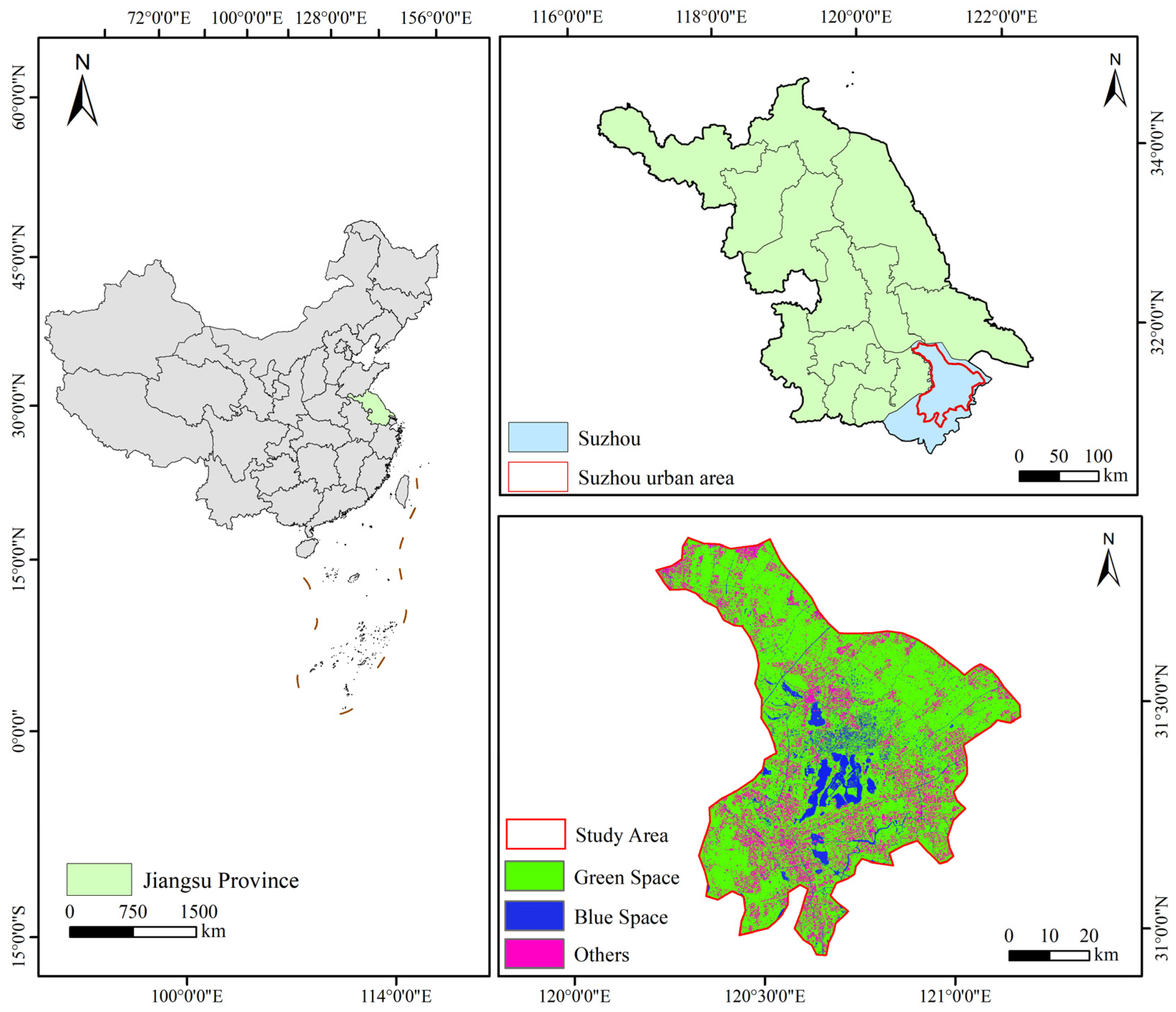
Figure 1. Overview of the built-up area in Suzhou, the study region.
Land 15 00618 g001
Figure 2. Research flowchart.
Land 15 00618 g002
Figure 3. Five-phase spatial distribution of LST in Suzhou’s built-up areas. LST is expressed in Kelvin (K) and represents the average LST over the June–October period for each study year. (a) 2000, (b) 2005, (c) 2010, (d) 2016, (e) 2022.
Land 15 00618 g003
Figure 4. Heatmap of BGs proportion under different LCZ types in Suzhou’s built-up areas during the five phases.
Land 15 00618 g004
Figure 5. Statistical diagram of BGs proportion versus LST regression slope across different LCZ types in Suzhou’s built-up areas during the five phases. (a) 2000, (b) 2005, (c) 2010, (d) 2016, (e) 2022.
Land 15 00618 g005
Figure 6. Scatter plot matrix of BGs_std versus LST across five phases of Suzhou’s built-up areas under different LCZs.
Land 15 00618 g006
Figure 7. Scatter plot matrix regression analysis of BGs_std versus LST across five phases of Suzhou’s built-up areas under different LCZ types.
Land 15 00618 g007
Figure 8. Statistical diagram of Pearson correlation coefficients between BGs_std and LST under different LCZ types across five phases in Suzhou’s built-up areas. * denotes significance.
Land 15 00618 g008
Disclaimer/Publisher’s Note: The statements, opinions and data contained in all publications are solely those of the individual author(s) and contributor(s) and not of MDPI and/or the editor(s). MDPI and/or the editor(s) disclaim responsibility for any injury to people or property resulting from any ideas, methods, instructions or products referred to in the content.