NGRDI-DCNLab: Integrating Spectral Prior and Deformable Convolution for Urban Green Space Extraction from High-Resolution RGB Remote Sensing Imagery

Abstract

Accurate urban green space (UGS) mapping is essential for assessing urban ecosystem health and supporting sustainable development planning. However, deep learning-based UGS segmentation from Red–Green–Blue (RGB) remote sensing imagery faces two major challenges. First, the absence of near-infrared (NIR) information in RGB imagery hinders the ability to discriminate spectrally similar classes, such as vegetation and non-vegetation. Second, conventional convolutions with fixed receptive fields struggle to model the complex and irregular boundaries characteristic of UGS. To address these challenges, this study combined the Normalized Green–Red Difference Index with the Deformable Convolutional Network Lab (NGRDI-DCNLab) model, a semantic segmentation model tailored specifically for RGB-only imagery. Based on the DeepLabV3+ framework, the model introduced three core improvements: (1) The Normalized Green–Red Difference Index (NGRDI) was incorporated to compensate for the absence of NIR information, enhancing the spectral separability of vegetation pixels. (2) Standard convolutions in the decoder were replaced with deformable convolutions, enabling the network to more effectively adapt to irregular boundaries of UGS. (3) An NGRDI-weighted loss function was designed to assign higher weights to challenging samples and uncertain boundary regions, guiding the model toward more accurate edge delineation. Comprehensive evaluations on two public high-resolution datasets—the Wuhan Dense Labeling Dataset (WHDLD) and the Beijing subset of the Urban Green Space-1m dataset (UGS-1m_Beijing)—demonstrated that the NGRDI-DCNLab model outperformed existing popular deep learning models (like Unet++, etc.). Specifically, the deformable convolution effectively enhances the feature modeling capability for irregular boundaries; incorporating the NGRDI vegetation index as a fourth channel strengthens spectral feature representation and improves the distinction between vegetation and non-vegetation; and adding the dynamic NGRDI-weighted loss enables targeted learning for challenging samples. Through the synergistic effect of these three modules, the model achieves mean Intersection over Union (MIoU) scores of 84.77% and 77.66%, as well as F1-scores of 91.75% and 87.27%, on the WHDLD and UGS-1m_Beijing datasets, respectively. Furthermore, the model exhibited certain generalization capability on the unmanned aerial vehicle (UAV) dataset, the Urban Drone Dataset 6 (UDD6), attaining an MIoU of 87.43%. Our results confirm that high-precision UGS extraction is achievable using only RGB remote sensing imagery, providing a cost-effective and practical technical solution for refined urban governance and ecological monitoring.

1. Introduction

Urban green spaces (UGSs) are a crucial component of urban systems, playing a significant role in mitigating the heat island effect, improving the urban environment, and enhancing residents’ quality of life [1,2]. Against the backdrop of rapid global urbanization, achieving efficient and accurate mapping of the spatial distribution of UGS has become an urgent need for supporting rational urban planning, promoting sustainable urban development, assisting government strategies, and deepening urban geographical research [3]. Remote sensing technology, particularly satellite remote sensing, provides the capability for large-scale, periodic observations. Traditionally, medium- to high-resolution remote sensing imagery such as the Landsat series has been widely used for large-scale land use and land cover change monitoring due to its broad coverage and continuous time series [4]. However, the spatial resolution of such imagery is limited (typically 30 m), making it difficult to effectively capture the fine-scale distribution characteristics of fragmented and scattered green spaces within cities [5].

In recent years, the proliferation of meter- to sub-meter-level high-resolution remote sensing imagery (e.g., domestic GaoFen series, WorldView, etc.) has provided a data foundation for fine-grained analysis of UGS [6]. Faced with massive and informationally complex high-resolution imagery, traditional machine learning-based methods have encountered bottlenecks in feature engineering complexity and model generalization capability [7]. Deep learning, especially semantic segmentation networks (e.g., U-Net, PSPNet, DeepLabV3+ and SegNet [8,9,10,11]), has become the mainstream technology in this field due to its powerful end-to-end feature learning capability. However, these general-purpose architectures are not specifically designed for UGS extraction. When confronted with inherent spectral heterogeneity (“same spectrum, different objects,” e.g., green roofs vs. vegetation, water bodies vs. shadows) and morphological complexity (irregular boundaries, fragmented distribution, multi-scale features), they often suffer from issues like blurred boundaries, loss of detail, and mis-segmentation.

To address these challenges, existing research has evolved primarily along two pathways. The first focuses on designing more powerful network architectures. For example, by employing multi-scale feature extraction modules to enhance segmentation accuracy [12,13,14], or by adopting dual encoders that parallelize convolutional neural networks (CNN) and Transformer to efficiently integrate global and local features [1,15,16]. The second pathway involves the fusion of multi-source data or features. The most typical strategy introduces imagery containing the near-infrared (NIR) band, calculates spectral indices such as the Normalized Difference Vegetation Index (NDVI), and fuses them with the original image as an additional channel to augment vegetation information [1,13,14]. Although this second pathway is effective, it heavily relies on the NIR band, which limits its applicability to data sources with only visible light bands. Currently, there is a large number of widely available data sources, including consumer-grade drone images, historical archived high-resolution satellite data, and numerous open-source satellite products. Most of these sources only contain RGB and do not have an NIR band. These data sources hold significant potential for applications in urban ecological monitoring, planning, and management. However, the absence of NIR information precludes the use of the NDVI for vegetation information extraction. This situation gives rise to unique challenges in urban green space extraction when relying solely on RGB data. The limited information content of RGB spectra for vegetation discrimination exacerbates the “same spectrum, different objects” phenomenon in urban scenes. Moreover, although existing semantic segmentation models designed for RGB imagery can model complex spatial configurations, they struggle to compensate for the inherent spectral deficiencies, leading to degraded segmentation performance for green spaces on RGB images. Consequently, achieving high-precision urban green space extraction from widely available, low-cost RGB imagery without reliance on NIR band remains a pressing challenge to be addressed. This not only lowers the barrier to data acquisition but also serves as an important pathway toward advancing fine-grained urban green space management.

To address the above issues, we systematically evaluate and integrate spectral prior and deformable convolution, establishing a methodologically rigorous and high-performance benchmark method for the practical challenge of high-precision green space extraction using only RGB data. Specifically, this paper proposes a semantic segmentation model for fine-grained UGS extraction from RGB remote sensing imagery, named NGRDI-DCNLab. The core objective of this research is to construct a systematic framework featuring collaborative spectral-spatial-optimization enhancement, tackling the challenge of RGB-based vegetation extraction in a closed-loop manner. Our main contributions are as follows:

• Spectral Prior-Enhanced Input. The Normalized Green–Red Difference Index (NGRDI) [17], calculated from RGB bands, is introduced as a fourth input channel. This explicitly injects physically interpretable spectral prior knowledge about vegetation into the network, enhancing the model’s fundamental discriminative power between vegetation and non-vegetation features at the source.
• Spatial Geometry-Adaptive Modeling. The decoder of DeepLabV3+ is improved by replacing standard convolutions with Deformable Convolutional Networks (DConv) [18]. This design endows the network with the ability to dynamically adjust the geometric shape of receptive fields, thereby enabling more precise fitting of the irregular and fragmented boundaries and internal structures of UGS.
• Objective-Oriented Dynamic Optimization. A novel dynamic weighted loss function based on NGRDI is innovatively designed. Utilizing the same spectral prior, this function adaptively increases the loss weight for challenging samples, such as those in vegetation–non-vegetation transition zones, during the training process. This guides the model to continuously focus on boundary refinement and the learning of difficult cases, forming a closed-loop feedback from feature input to optimization objective.

Crucially, these three modules do not operate in isolation; rather, they constitute a synergistically enhanced closed-loop system. The spectral prior guides both the spatially adaptive modeling and the optimization target, while the dynamic optimization, in turn, drives the model to better utilize spectral and geometric information. This closed-loop design enables the framework to systematically address the dual challenges of spectral confusion and geometric complexity in RGB imagery.

2. Datasets

The experimental evaluation in this study was performed on two publicly available benchmark datasets: the Wuhan Dense Labeling Dataset (WHDLD) and the Beijing subset of the Urban Green Space-1m dataset (UGS-1m_Beijing). All samples were uniformly and randomly partitioned into training, validation, and test datasets following the standard ratio of 70%:15%:15%. This strategy provided sufficient data for model learning, enables precise hyperparameter tuning using the validation dataset, and supported a statistically sound assessment of model performance on an independent test set, thereby ensuring the robustness and objectivity of the experimental results.

2.1. WHDLD

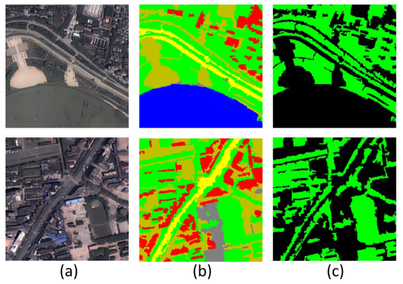
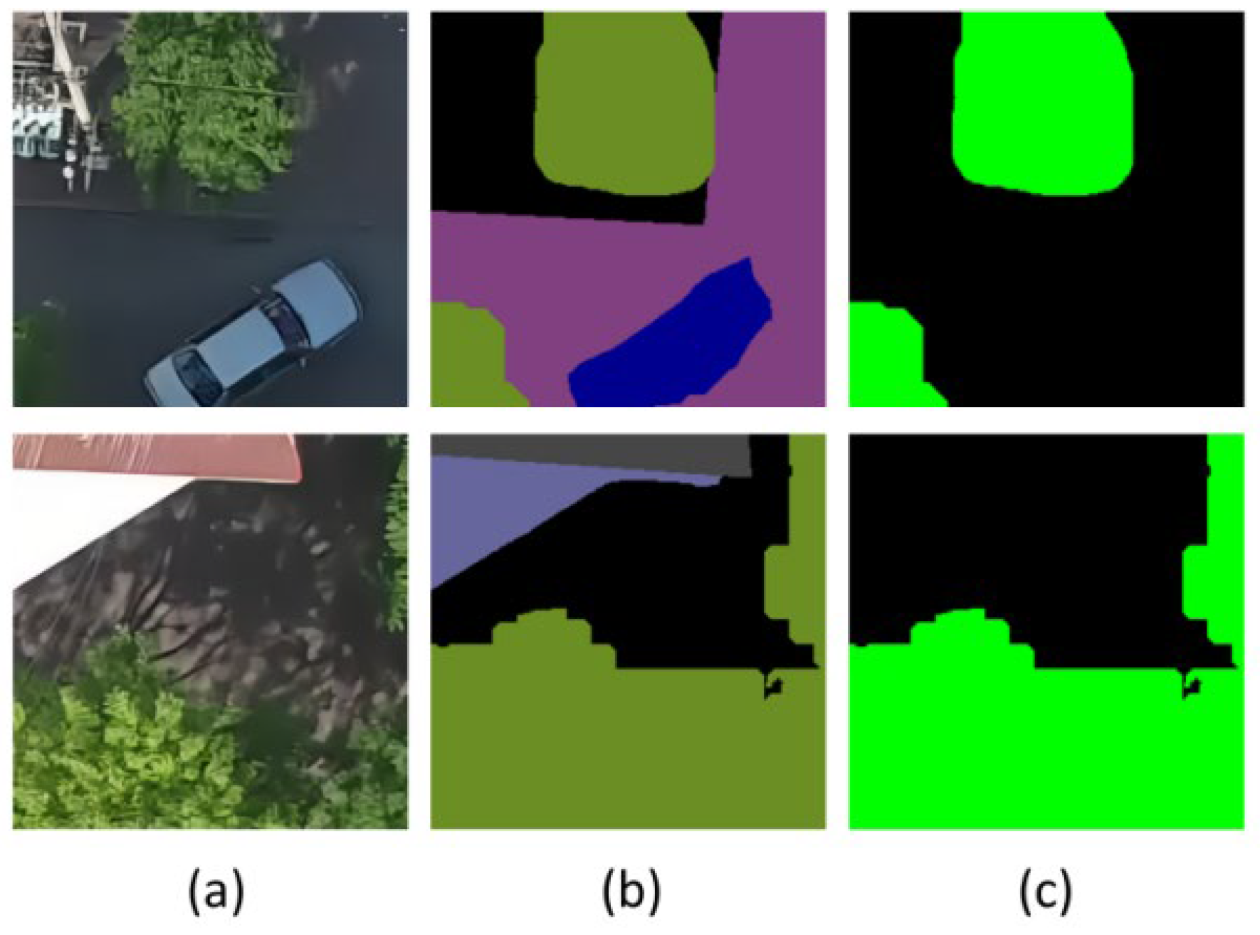
The WHDLD is a densely annotated high-resolution remote sensing dataset [19], consisting of 4940 images with a spatial resolution of 2 m and dimensions of 256 $\times$ 256 pixels. The dataset originally contains six land-cover categories: building, road, vegetation, sidewalk, barren land and water. For the purposes of this study, all non-vegetation categories were merged into a single background class, transforming the WHDLD into a binary classification dataset tailored for UGS extraction, as illustrated by the sample shown in Figure 1. Following the predefined data split, the numbers of image pairs for the training, validation and test sets are 3485, 741 and 741, respectively.

2.2. UGS-1m_Beijing Dataset

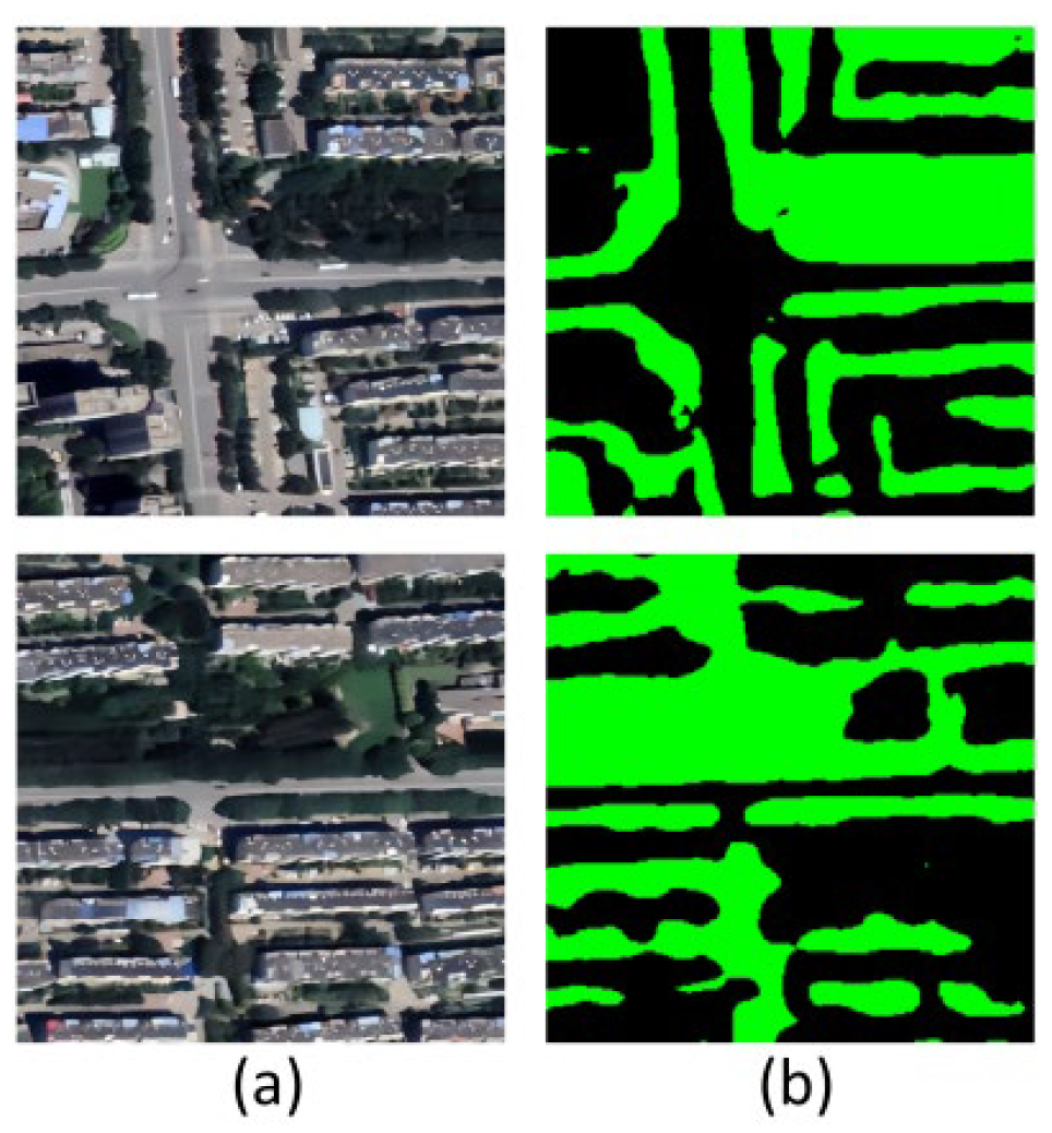
The UGS-1m_Beijing dataset is derived from the UGS-1m dataset released in 2023 [20]. The original dataset was constructed from Google Earth imagery with an approximate spatial resolution of 1 m and provides fine-grained annotations of UGS distribution across 31 major cities in China. To match the regional focus and experimental requirements of this study, image data from Beijing’s Dongcheng, Xicheng and Chaoyang districts were extracted to form the UGS-1m_Beijing subset. All selected images and their corresponding labels were uniformly cropped into standardized 256 $\times$ 256 pixels samples. To ensure sufficient variability and prevent overly simple or extreme cases, samples with UGS coverage below 30% (too low) or above 90% (too high) were removed. After filtering, a total of 9566 valid samples remained (an example is shown in Figure 2). The dataset was partitioned into training (6696), validation (1435) and test (1435) sets following the 70%:15%:15% ratio.

3. Methodology

The NGRDI-DCNLab model proposes a comprehensive and collaboratively optimized solution to the two core challenges of RGB-based UGS extraction (spectral confusion and geometrically blurred boundaries). The proposed approach enhances the entire processing pipeline. At the input stage, it explicitly incorporates prior vegetation spectral knowledge to improve feature separability. At the architectural level, it strengthens geometric modeling capability for irregular boundaries. In the optimization stage, it applies a dynamic weighting strategy to emphasize learning from challenging samples. Together, these components form a holistic, co-designed framework covering feature acquisition, semantic representation and optimization objectives.

3.1. Overall Framework

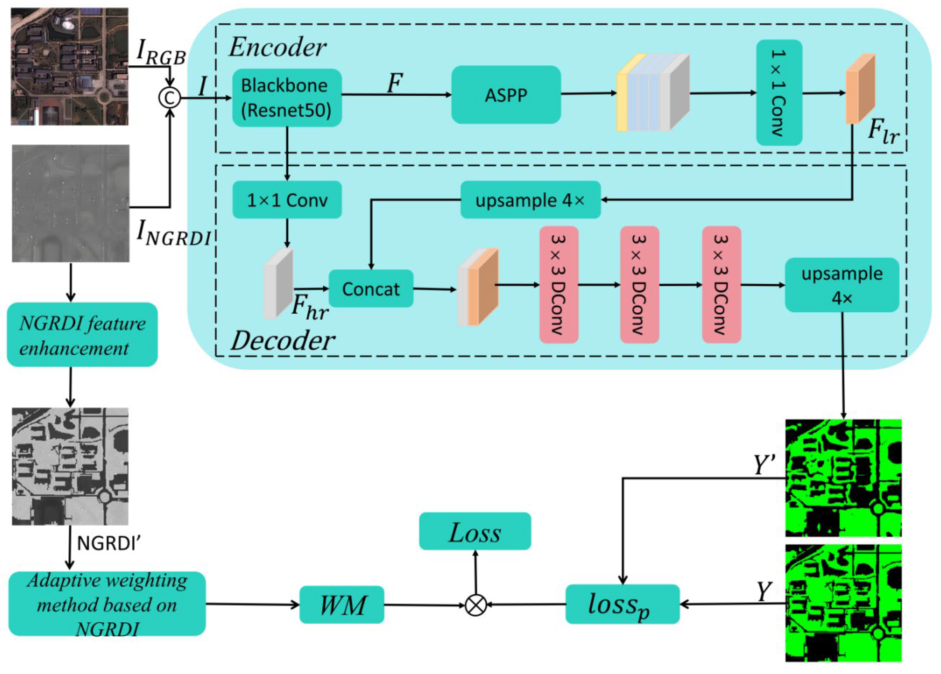
As illustrated in Figure 3, NGRDI-DCNLab adopts a classic encoder–decoder architecture [21] and consists of three major components: (1) an NGRDI-augmented four-channel input module that injects prior vegetation spectral information; (2) a decoder enhanced with deformable convolutions to improve fine-grained modeling of irregular green-space boundaries; (3) a dynamic weighted loss module that leverages both spectral priors and prediction confidence to enable progressive and adaptive optimization.

3.2. Detailed Network Architecture

3.2.1. NGRDI-Driven Four-Channel Input

To compensate for the absence of a NIR band in visible spectral remote sensing imagery [22], this study incorporates the NGRDI as prior vegetation spectral knowledge. Specifically, a single-channel NGRDI map $I_{NGRDI}$ is first calculated from the original RGB image using Equation (1):

$$\mathit{NGRDI} = {\displaystyle \frac{ G-R }{G+\mathit{R}}}$$

(1)

where $G$ and $R$ represent the pixel values in the green and red bands, respectively [23]. This map is then concatenated with the RGB channels along the channel dimension to construct a four-channel input tensor, as shown in Equation (2):

$$\mathit{I} = \mathit{Concat}\left({\mathit{I}}_{\mathit{RGB}} , {\mathit{I}}_{\mathit{NGRDI}}\right)$$

(2)

Although deep convolutional neural networks (DCNNs) theoretically have the capacity to approximate any function, this study explicitly incorporates NGRDI as a fourth input channel based on two key theoretical considerations:

• Inductive Bias from Arithmetic Operations. The core operators of standard CNN are convolution (multiply-accumulate operations) and activation functions [24], which are inherently inefficient at capturing the division operation that defines the NGRDI. Approximating such a non-linear ratio solely through stacked convolutional layers is parameter-inefficient and prone to converging to suboptimal local minima. By explicitly computing NGRDI, the model is endowed with a targeted inductive bias, directly supplying a higher-order non-linear representation of vegetation spectral properties and thus reducing the network’s learning burden;
• Enhancing Feature Discriminability. In urban landscapes, vegetation in the original RGB spectral space is susceptible to confusion with artificial materials such as specific roofs or pavements [25]. The NGRDI, calculated as a normalized difference between the green and red bands, serves to enhance the unique reflectance signature of vegetation. By explicitly providing this index as an input, the model’s ability to distinguish spectrally similar objects (“different objects with similar spectra”) is improved at the data source.

3.2.2. Encoder–Decoder Structure

The primary function of the encoder is to extract hierarchical spectral-spatial features from the four-channel input. Specifically, a ResNet50 backbone [26], pre-trained on ImageNet, is adopted to efficiently capture deep semantic representations and global contextual information. The input tensor $\mathrm{I}$ is first processed by the backbone to produce low-resolution feature maps $F$ enriched with high-level context. These features are then passed into an Atrous Spatial Pyramid Pooling (ASPP) module, which employs parallel atrous convolutions with varying dilation rates to capture multi-scale contextual information [27]. This design effectively mitigates the challenge posed by the diverse spatial scales of UGS. The outputs of the ASPP module are subsequently fused and compressed through a 1 $\times$ 1 convolution to generate the final low-resolution semantic feature map $F_{lr}$.

3.2.3. Deformable Decoder for Boundary Refinement

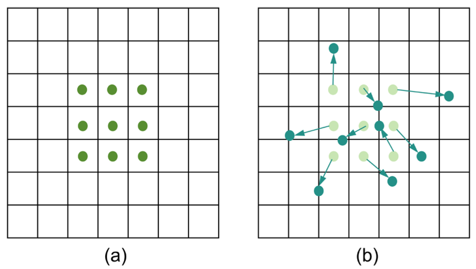
The decoder is responsible for upsampling the low-resolution semantic feature map ${ F}_{lr}$ back to the original input resolution while precisely refining UGS boundaries. UGS boundaries are typically irregular and often intertwined with man-made structures such as roads and buildings. Standard convolutions, constrained by their fixed geometric sampling grids (as shown in Figure 4a), exhibit rigid sampling point distributions that cannot be dynamically adjusted based on the input content. This limitation hinders their ability to accurately represent such complex morphologies, frequently resulting in blurred segmentation edges and shape distortion [28]. To overcome this limitation, this study introduces a key improvement to the DeepLabV3+ decoder by replacing its standard 3 $\times$ 3 convolutions with DConv (as shown in Figure 4b). Unlike standard convolutions, DConv is not confined to a fixed grid topology. Instead, it adaptively learns a 2D offset for each convolutional sampling point (the dark green arrows indicate the direction and magnitude of the offset), enabling the sampling grid to dynamically deform according to the geometric properties of the target objects [29]. Given the intricate spatial arrangement of urban features like buildings and green spaces, this flexible receptive field provided by DConv allows the model to better “fit” the actual contours of green spaces. Consequently, it substantially enhances the delineation of building edges, fragmented vegetation patches, and highly irregular boundaries during the decoding stage. Ultimately, the decoder integrates high-level, low-resolution semantic features $F_{lr}$ from the encoder with shallow, high-resolution features $F_{hr}$ from early backbone layers to generate the final segmentation prediction map $Y^{\prime }$.

3.3. Dynamic Weighted Loss

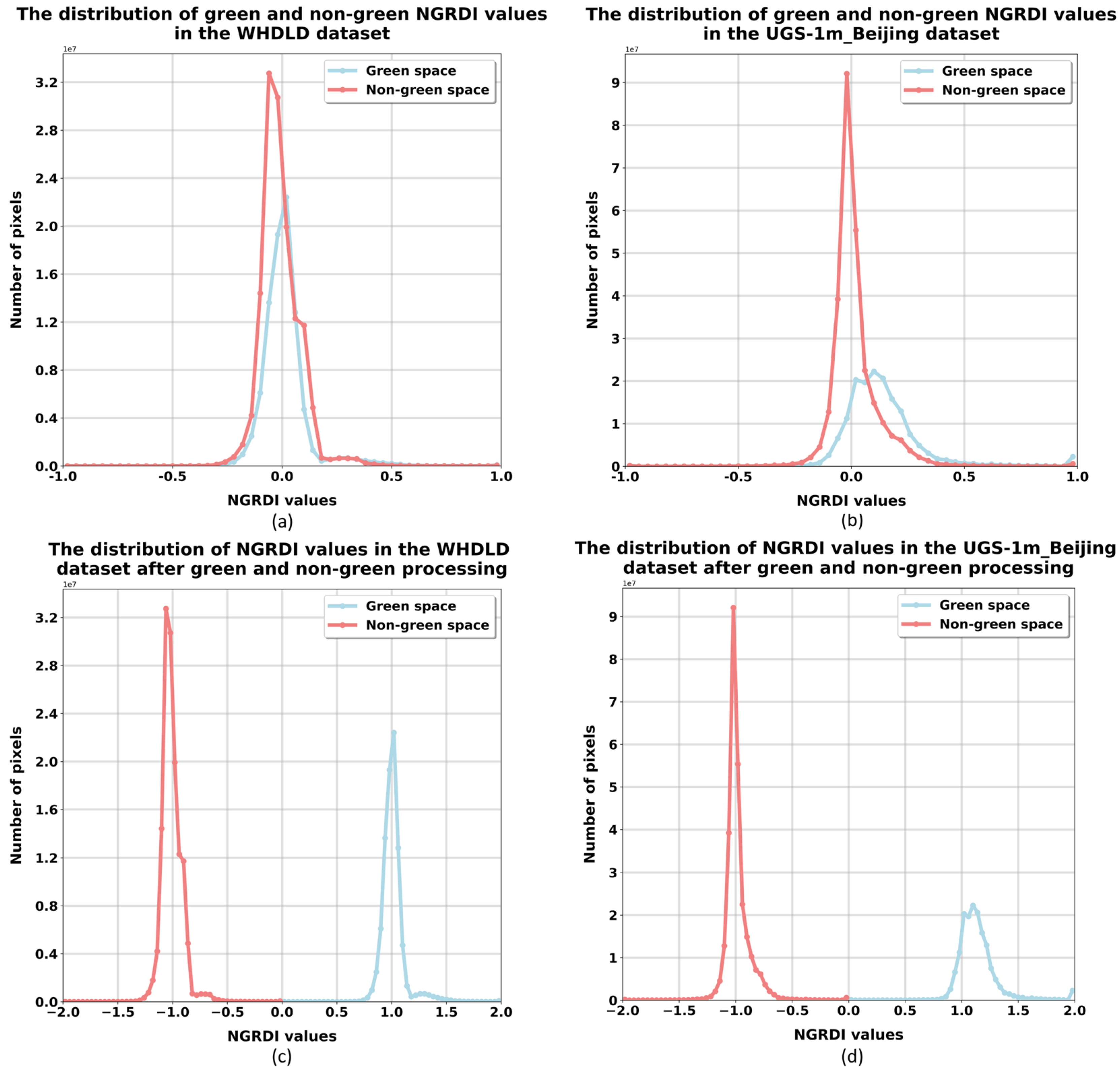
Figure 5 illustrates the distributions of NGRDI values for green and non-green in the WHDLD and UGS-1m_Beijing training datasets. As illustrated in Figure 5a,b, substantial spectral overlap exists between green and non-green regions in 8-bit RGB imagery, and boundary pixels exhibit particularly high prediction uncertainty. Under such conditions, a fixed-weight cross-entropy loss is unable to effectively balance the learning of easy and hard samples. To overcome this limitation, we introduce a dynamic weighting strategy that incorporates both spectral priors and prediction confidence, enabling progressive enhancement of learning for typical and challenging samples across training phases. The proposed loss function integrates a fundamental pixel-wise binary cross-entropy term with a phased dynamic weighting component.

3.3.1. Base Loss Function

The pixel-wise binary cross-entropy serves as the foundational component of the entire loss function, measuring the discrepancy between the model’s predicted probabilities and the ground truth labels [30]. Let $y_{(i,j)}\in \{\mathrm{0,1}\}$ be the ground truth label for the pixel $(i,j)$ and $p_{(i,j)}$ be the model’s predicted probability of it belonging to green space. This base loss function is defined by Equation (3):

$${loss}_p\left(i,j\right)= -\left[ y_{(i,j)}·\mathit{log}\left(p_{(i,j)}\right)+ \left(1-y_{(i,j)}\right)·\mathit{log}\left(1-p_{(i,j)}\right)\right]$$

(3)

3.3.2. Adaptive Loss Function

The conventional cross-entropy loss assigns equal importance to all pixels, making it difficult to cope with the uneven segmentation difficulty inherent in complex urban remote sensing scenes. To encourage the model to concentrate on more challenging pixels, this study introduces an NGRDI-based adaptive weighting strategy. This approach constructs a spectral Weight Map that dynamically adjusts each pixel’s contribution to the loss according to its segmentation difficulty.

However, direct use of the original NGRDI can lead to weighting failure due to the overlapping value ranges between vegetation and certain dark non-vegetated surfaces. To mitigate this issue, we generate an enhanced NGRDI feature ${NGRDI}_{(i,j)}^{\prime }$ using the ground-truth labels, as defined in Equation (4):

$${NGRDI}_{(i,j)}^{\prime }=\{\begin{array}{c}NGRDI(i,j)+∆,{ y}_{i,j}=1,\\ NGRDI(i,j)-∆, y_{i,j}=0.\end{array}$$

(4)

where $∆$ is determined by the NGRDI range [$a$,$b$] of the training set, and its formula is defined as

$$∆={\displaystyle \frac{(b-a)}{2}}$$

(5)

This operation effectively enlarges the spectral-domain separation between green and non-green regions, as illustrated in Figure 5c,d.

Building on this enhanced feature, the spectral weight for each pixel is then defined. A Gaussian function is applied to assign adaptive weights to vegetation pixels, while non-vegetation pixels are assigned a baseline weight. The complete formulation is provided in Equation (6):

$$W_{spec}(i,j)=\{\begin{array}{c}1+A·exp(-{\displaystyle \frac{{({NGRDI}_{(i,j)}^{\prime }-{\mu }_g)}^2}{2{{\sigma }_g}^2}}), y_{i,j}=1,\\ 1, y_{i,j}=0.\end{array}$$

(6)

where ${\mu }_g$ and ${\sigma }_g$ are the mean and standard deviation, respectively, of the NGRDI values for all green space pixels in the training dataset.

3.3.3. Three-Phase Dynamic Training Strategy

To ensure training stability and promote targeted learning, this study divides the training process into three distinct phases, enabling progressive optimization from “typical sample learning” to “hard sample enhancement” and finally to “uncertain sample refinement”. We couple the weighting factor $A$ with the training epoch to construct a three-phase dynamic training strategy. Let $\mathrm{T}$ denote the total number of epochs and $t$ represent the current epoch. A mask function $M(i,j,t)\mathsf{ϵ}\left\{\mathrm{0,1}\right\}$ is introduced to indicate whether pixel $(i,j)$ participates in the weight calculation. The final weight is defined as

$$W(i,j,t)=1+M(i,j,t)·\left(W_{spec}\right(i,j)-1)$$

(7)

where $W_{spec}(i,j)$ represents the spectral weight of the pixel at $(i,j)$. The weighting coefficients $A\left(t\right)$ are dynamically adjusted following the procedure is described in Algorithm 1. The hyperparameters used in Algorithm 1 (e.g., 0.25T, 0.65) are determined based on the general principles of Curriculum Learning and empirical observations of prediction confidence throughout the training process [31].

Finally, the total loss ($Loss$) is computed from the weighted pixel-wise loss, as defined in Equation (8):

$$Loss={\displaystyle \frac{1}{N}}{\sum }_{i,j}W(i,j,t)·{loss}_p\left(i,j\right)$$

(8)

where N represents the total number of pixels.

Algorithm 1 Three-Stage Dynamic Training Strategy

Input: Training samples composed of images and their corresponding segmented ground truth labels{$(I,Y)$}, total epochs $T$, $A_{\mathrm{m}\mathrm{a}\mathrm{x}}=1.5$, spectral weight matrix $W_{\mathrm{s}\mathrm{p}\mathrm{e}\mathrm{c}}$.

Output: Dynamic weights $W(i,j,t)$ for each pixel across training stages.

1: Initialize current epoch $t=0$.

2: While $t<T$ do

3:          Sample a minibatch from {$(I,Y)$}; compute prediction probabilities $p(i,j,t)$ via                model forward pass.

4:           Determine stage and compute $A\left(t\right)$, $M(i,j,t)$

5:           If $t<0.25 T$ then

6:                   $A\left(t\right)=1.5·t/\left(0.25T\right)$; $M(i,j,t)=1(y_{i,j}=1)$

7:           else if 0.25$T$ < $t$ < 0.85$T$ then

8:                   $A\left(t\right)=1.5$; $M(i,j,t)=1(y_{i,j}=1\cap (p(i,j,t)<0.65)\cup p(i,j,t)\ne y_{i,j})$

9:           else

10:                   $A\left(t\right)=1.5·(T-t)/\left(0.15T\right)$; $M(i,j,t)=1(0.3<p(i,j,t)<0.7)$

11:           end if

12:           Compute dynamic weight: $W(i,j,t)$ = 1 + $M(i,j,t)·{(W}_{\mathrm{s}\mathrm{p}\mathrm{e}\mathrm{c}}(i,j)-1)$.

13:           Train model with weighted loss (using $W(i,j,t)$ and $A\left(t\right)$ on the minibatch.)

14:           $t=t+1$

15: End While

16: Return $W(i,j,t)$

4. Experiments

4.1. Experimental Setup and Evaluation Metrics

The experiments were conducted on a Linux platform equipped with an NVIDIA GeForce RTX 4090 GPU (NVIDIA Corporation, Santa Clara, CA, USA) featuring 24 GB VRAM. The network was trained with a batch size of 16 for 80 epochs on both the WHDLD and UGS-1m_Beijing datasets. The base learning rate was set to 0.01, and a “poly” learning rate policy with a power of 0.9 was employed. Model optimization was performed using Stochastic Gradient Descent with a cross-entropy loss function. For data augmentation, the training dataset underwent random scaling, cropping and horizontal flipping, followed by normalization. The validation dataset was processed with only standardization and resizing to ensure consistent and stable evaluation. A fixed random seed of 1 was used to guarantee the reproducibility of all stochastic components, including data shuffling, augmentation operations and model initialization.

Five core metrics were employed for quantitative evaluation: Overall Accuracy (OA), Mean Pixel Accuracy (MPA), Mean Intersection over Union (MIoU), F1-Score and Frequency Weighted Intersection over Union (FWIoU). OA measures the overall correctness of classification results [32]. MPA mitigates class imbalance by averaging the accuracy across classes [33]. MIoU quantifies the overlap between the predicted and ground-truth green space pixels [34]. The F1-Score provides a balanced assessment of precision and recall in green space extraction [35]. FWIoU further accounts for class imbalance by weighting the IoU of each class according to its pixel frequency [36]. The mathematical formulations of these metrics are given as follows:

$$\mathrm{O}\mathrm{A}={\displaystyle \frac{{\sum }_{\mathrm{i}=0}^{\mathrm{k}}{\mathrm{p}}_{\mathrm{i}\mathrm{i}}}{{\sum }_{\mathrm{i}=0}^{\mathrm{k}}{\sum }_{\mathrm{j}=0}^{\mathrm{k}}{\mathrm{p}}_{\mathrm{i}\mathrm{j}}}}$$

(9)

$$\mathrm{M}\mathrm{P}\mathrm{A}={\displaystyle \frac{1}{\mathrm{k}+1}}{\sum }_{\mathrm{i}=0}^{\mathrm{k}}{\displaystyle \frac{{\mathrm{p}}_{\mathrm{i}\mathrm{i}}}{{\sum }_{\mathrm{j}=0}^{\mathrm{k}}{\mathrm{p}}_{\mathrm{i}\mathrm{j}}}}$$

(10)

$$\mathrm{M}\mathrm{I}\mathrm{o}\mathrm{U}={\displaystyle \frac{1}{\mathrm{k}+1}}{\sum }_{\mathrm{i}=0}^{\mathrm{k}}{\displaystyle \frac{{\mathrm{p}}_{\mathrm{i}\mathrm{i}}}{{\sum }_{\mathrm{j}=0}^{\mathrm{k}}{\mathrm{p}}_{\mathrm{i}\mathrm{j}}+{\sum }_{\mathrm{j}=0}^{\mathrm{k}}{\mathrm{p}}_{\mathrm{j}\mathrm{i}}-{\mathrm{p}}_{\mathrm{i}\mathrm{i}}}}$$

(11)

$$\mathrm{P}={\displaystyle \frac{{\mathrm{p}}_{\mathrm{i}\mathrm{i}}}{{\mathrm{p}}_{\mathrm{i}\mathrm{i}}+{\mathrm{p}}_{\mathrm{i}\mathrm{j}}}}$$

(12)

$$\mathrm{R}={\displaystyle \frac{{\mathrm{p}}_{\mathrm{i}\mathrm{i}}}{{\mathrm{p}}_{\mathrm{i}\mathrm{i}}+{\mathrm{p}}_{\mathrm{j}\mathrm{i}}}}$$

(13)

$$\mathrm{F}1=2·{\displaystyle \frac{\mathrm{P}·\mathrm{R}}{\mathrm{P}+\mathrm{R}}}$$

(14)

$$\mathrm{F}\mathrm{W}\mathrm{I}\mathrm{o}\mathrm{U}={\displaystyle \frac{1}{{\sum }_{\mathrm{i}=0}^{\mathrm{k}}{\sum }_{\mathrm{j}=0}^{\mathrm{k}}{\mathrm{p}}_{\mathrm{i}\mathrm{j}}}}{\sum }_{\mathrm{i}=0}^{\mathrm{k}}{\displaystyle \frac{{\sum }_{\mathrm{j}=0}^{\mathrm{k}}{\mathrm{p}}_{\mathrm{i}\mathrm{j}}·{\mathrm{p}}_{\mathrm{i}\mathrm{i}}}{{\sum }_{\mathrm{j}=0}^{\mathrm{k}}{\mathrm{p}}_{\mathrm{i}\mathrm{j}}+{\sum }_{\mathrm{j}=0}^{\mathrm{k}}{\mathrm{p}}_{\mathrm{j}\mathrm{i}}-{\mathrm{p}}_{\mathrm{i}\mathrm{i}}}}$$

(15)

where ${\mathrm{p}}_{\mathrm{i}\mathrm{i}}$, ${\mathrm{p}}_{\mathrm{j}\mathrm{i}}$, ${\mathrm{p}}_{\mathrm{i}\mathrm{j}}$ and ${\mathrm{p}}_{\mathrm{j}\mathrm{j}}$ denote true and false positives, false and true negatives, respectively; k represents the number of object categories that are excluded from the background; Precision (P) indicates the proportion of samples that are actually classified into a specific category by the model; Recall (R) rate indicates the proportion of samples that truly belong to a specific category and are correctly identified by the model.

Additionally, to enable a more refined evaluation of the model’s accuracy in segmenting green space boundaries, this paper introduces the Boundary IoU (BIoU) metric. BIoU calculates the Intersection over Union of pixel sets within a specified distance d from the predicted and ground truth boundaries. This allows it to effectively reflect the prediction quality in boundary regions and exhibit greater sensitivity to minor boundary deviations [37]. The calculation formula is presented as follows.

$$\mathrm{B}\mathit{I}\mathrm{o}\mathrm{U}={\displaystyle \frac{\left|\right(\mathrm{G}\mathrm{d}\cap \mathrm{G})\cap (\mathrm{P}\mathrm{d}\cap \mathrm{P}\left)\right|}{\left|\right(\mathrm{G}\mathrm{d}\cap \mathrm{G})\cup (\mathrm{P}\mathrm{d}\cap \mathrm{P}\left)\right|}}$$

(16)

where G and P represent the ground truth mask and the predicted mask, respectively, and Gd and Pd denote the sets of pixels within d pixels from the ground truth contour and the predicted contour. To mitigate the impact of missed detections on the BIoU calculation, d is set to 3 pixels.

4.2. Comparative Analysis of Different Models

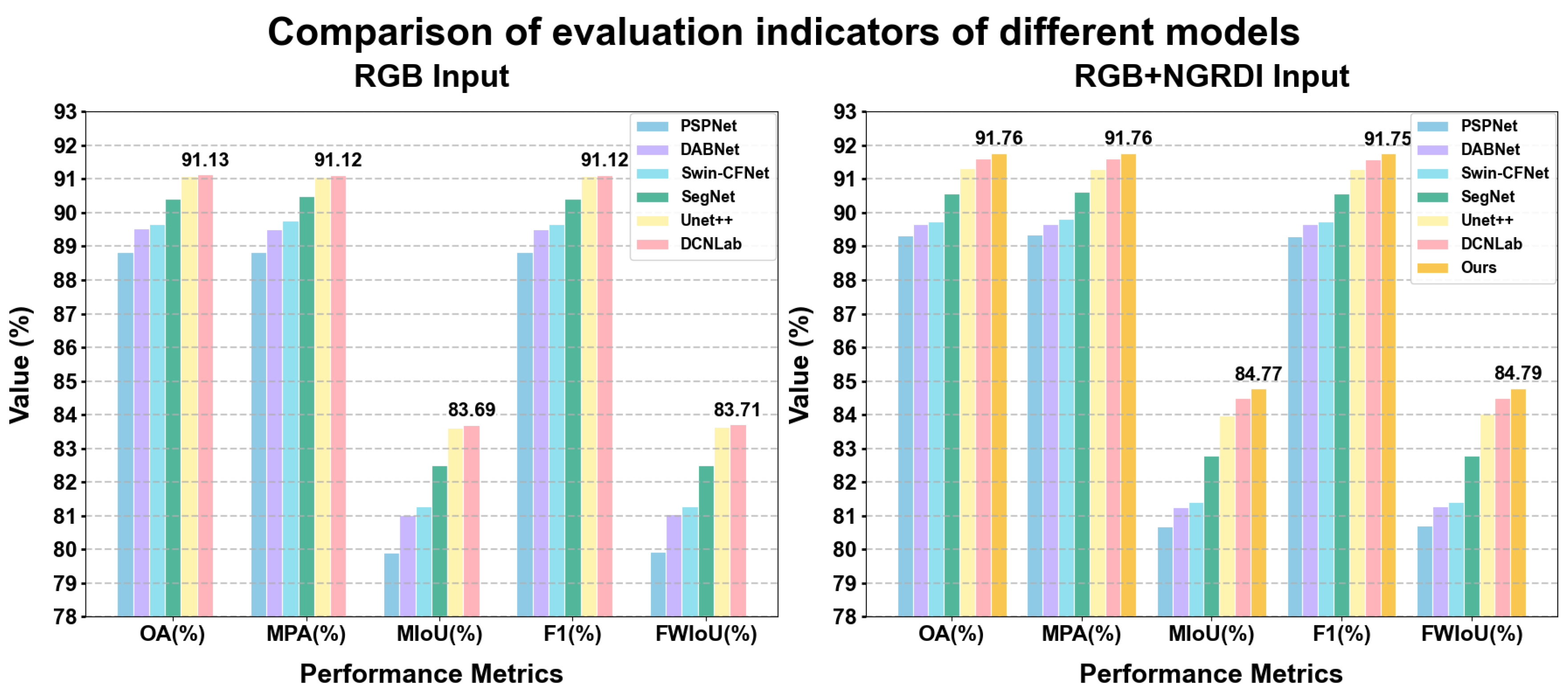
This study employed PSPNet, DABNet, SegNet, Swin-CFNet and UNet++ as benchmark models for comparative experiments. The evaluation metrics of these models on the WHDLD are summarized in Figure 6 (detailed numerical results are provided in Appendix A 

Table A1. Comparison of Different Models.

Method	RGB					RGB + NGRDI
	OA (%)	MPA (%)	MIoU (%)	F1 (%)	FWIoU (%)	OA (%)	MPA (%)	MIoU (%)	F1 (%)	FWIoU (%)
PSPNet	88.83	88.84	79.90	88.82	79.92	89.32	89.35	80.69	89.31	80.71
DABNet	89.52	89.50	81.02	89.51	81.04	89.67	89.66	81.26	89.66	81.29
Swin-CFNet	89.67	89.77	81.27	89.67	81.28	89.74	89.82	81.40	89.74	81.40
SegNet	90.40	90.50	82.49	90.40	82.49	90.58	90.63	82.78	90.58	82.79
Unet++	91.09	91.07	83.62	91.08	83.65	91.31	91.29	83.99	91.30	84.02
DconvLab	91.13	91.12	83.69	91.12	83.71	91.60	91.60	84.49	91.59	84.50
NGRDI-DCNLab	——	——	——	——	——	91.76	91.76	84.77	91.75	84.79

). Using only the standard three-channel RGB input, the proposed DCNLab model outperformed all competing networks across all metrics, achieving an OA of 91.13%, MPA of 91.12%, MIoU of 83.69%, F1-Score of 91.12% and FWIoU of 83.71%. Furthermore, incorporating the NGRDI vegetation index as a fourth input channel consistently improved the performance of all baseline models, highlighting the positive contribution of explicit vegetation spectral information.

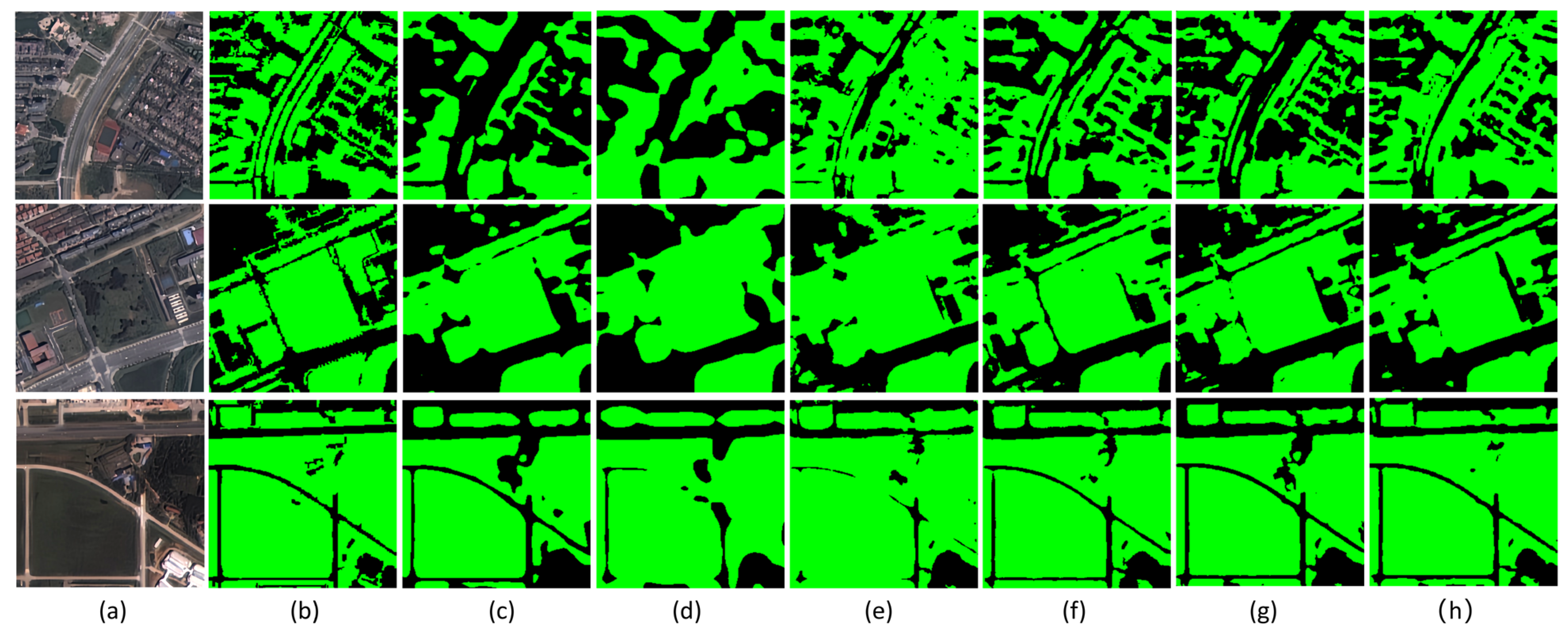
Figure 7 presents the semantic segmentation results of the comparison models. PSPNet exhibits noticeable regional fragmentation and blurred boundaries, indicating insufficient capability in delineating complex object edges. DABNet performs poorly in areas with dense buildings or intricate textures. SegNet is able to capture the general contours of features objects but struggles with fine structural details such as small buildings and road intersections. Swin-CFNet, based on a dual-encoder architecture, effectively captures multi-scale contextual information, showing notable improvement in detail preservation over the aforementioned models, but still has room for enhancement in handling complex boundaries and extremely small objects. UNet++, benefiting from nested skip connections, shows improved detail preservation over the aforementioned models, effectively identifying medium-sized green spaces and producing clearer boundaries, though it still encounters minor misclassifications in complex textured regions and has difficulty detecting very small green patches. However, it still encounters minor misclassifications in complex texture regions and has difficulty detecting very small green patches. In contrast, the proposed DCNLab model accurately identifies most UGS, delineates building and road boundaries more faithfully to the ground truth, and effectively overcomes the shortcomings observed in the other models, including detail loss and boundary distortions.

4.3. Ablation Experiment

This paper conducted systematic ablation experiments (results are presented in

Table 1. Statistics of ablation experiment performance for the WHDLD and UGS-1m_Beijing datasets.

Method	WHDLD					UGS-1m_Beijing
	OA (%)	MPA (%)	MIoU (%)	F1 (%)	FWIoU (%)	OA (%)	MPA (%)	MIoU (%)	F1 (%)	FWIoU (%)
Baseline	90.86	90.85	83.24	90.85	83.26	87.71	85.51	75.63	85.90	78.31
Baseline + DConv	91.13	91.12	83.69	91.12	83.71	88.10	86.00	76.32	86.36	78.92
Baseline + NGRDI	91.48	91.46	84.28	91.47	84.30	88.35	86.43	76.80	86.68	79.33
Baseline + DConv + NGRDI	91.60	91.60	84.49	91.59	84.50	88.64	86.59	77.25	86.97	79.78
Baseline + DConv + NGRDI + W	91.76	91.76	84.77	91.75	84.79	88.68	87.63	77.66	87.27	79.97

) to individually validate and analyze the proposed DConv, NGRDI, and dynamic Weighted loss modules on the WHDLD and UGS-1m_Beijing datasets. Using DeepLabV3+ (with ResNet50 as the backbone) as the baseline model, the experimental results demonstrate that each module effectively improves model performance, with their synergistic effect being significant. Compared to the baseline, the separate introduction of DConv yielded MIoU improvements of 0.45% and 0.69% on the two datasets, respectively, indicating DConv’s adaptive fitting capability for complex geometric boundaries. It effectively reduces the boundary roughness and distortion caused by standard convolutions when processing features like the jagged contours at the interface between buildings and green spaces or the edges of narrow green belts. The separate introduction of the NGRDI vegetation index as a fourth input channel led to more substantial performance gains (MIoU improvements of 1.04% and 1.17%, respectively), enhancing the model’s robustness against the inherent spectral confusion in RGB imagery. Combining DConv with NGRDI achieved further synergistic improvement (MIoU gains of 1.25% and 1.62%, respectively), suggesting that the adaptation of spatial geometry and the enhancement of spectral discriminative power are complementary. The clear spectral prior provides explicit semantic guidance for the deformation learning in DConv. Finally, introducing the NGRDI-based dynamic Weighted loss module enabled the model to achieve optimal performance (total MIoU improvements of 1.53% and 2.03%), as this loss function forces the model to focus on challenging samples, such as the ambiguous vegetation–non-vegetation transition zones and small patches with uncertain NGRDI values, thereby enabling targeted optimization of segmentation “shortcomings.” The specific improvements contributed by each module concerning boundary geometry, spectral discrimination, and hard case learning will be visually presented and analyzed in detail through comparative experiments in Section 4.4, Section 4.5 and Section 4.6.

4.4. Comparative Experiments on Deformable Convolutions

This section presents a comparative analysis conducted on the WHDLD and UGS-1m_Beijing datasets using the DeepLabV3+ architecture with a ResNet50 backbone. Specifically, the 3 $\times$ 3 convolution in the decoder was replaced with DConv, and its performance was compared against standard 3 $\times$ 3 convolution, with the results summarized in

Table 2. Comparison of segmentation performance using different convolutions types on the WHDLD and UGS-1m_Beijing datasets.

Method	WHDLD						UGS-1m_Beijing
	OA (%)	MPA (%)	MIoU (%)	F1 (%)	FWIoU (%)	BIoU (%)	OA (%)	MPA (%)	MIoU (%)	F1 (%)	FWIoU (%)	BIoU (%)
DeepLabV3+ (ResNet50)	90.86	90.85	83.24	90.85	83.26	37.13	87.71	85.51	75.63	85.90	78.31	28.40
DCNLab	91.13	91.12	83.69	91.12	83.71	37.96	88.10	86.00	76.32	86.36	78.92	30.26

. As illustrated in Table 2, integrating 3 $\times$ 3 DConv into the decoder outperforms standard 3 $\times$ 3 convolution, improving the MIoU by 0.45% on the WHDLD and 0.69% on the UGS-1m_Beijing dataset, and the BIoU by 0.83% and 1.86%, respectively. This indicates that DConv can more accurately fit urban green space boundaries, effectively reducing misclassifications in boundary regions.

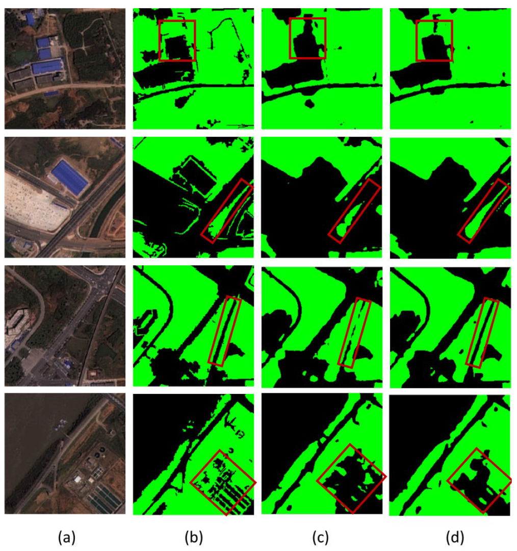
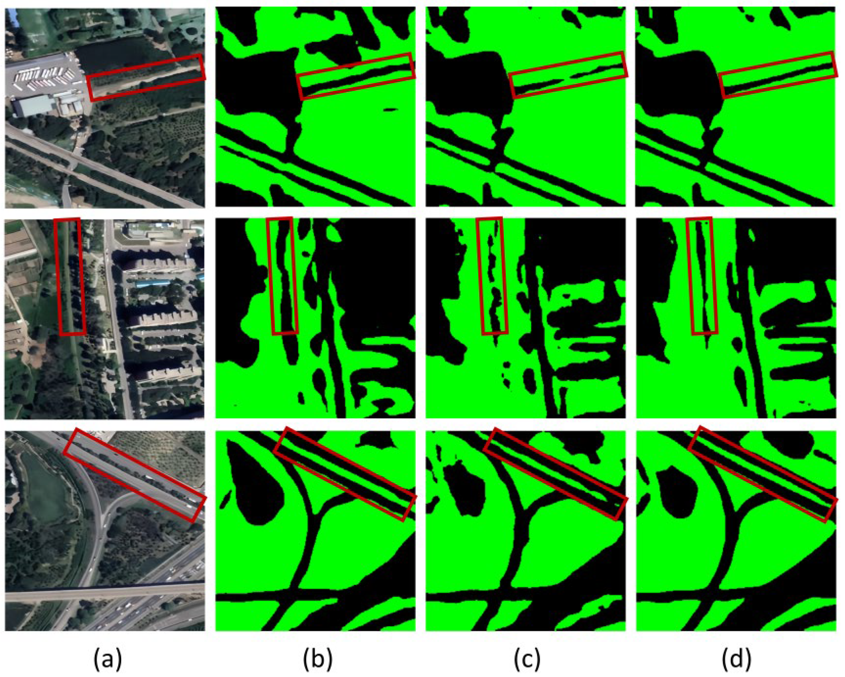
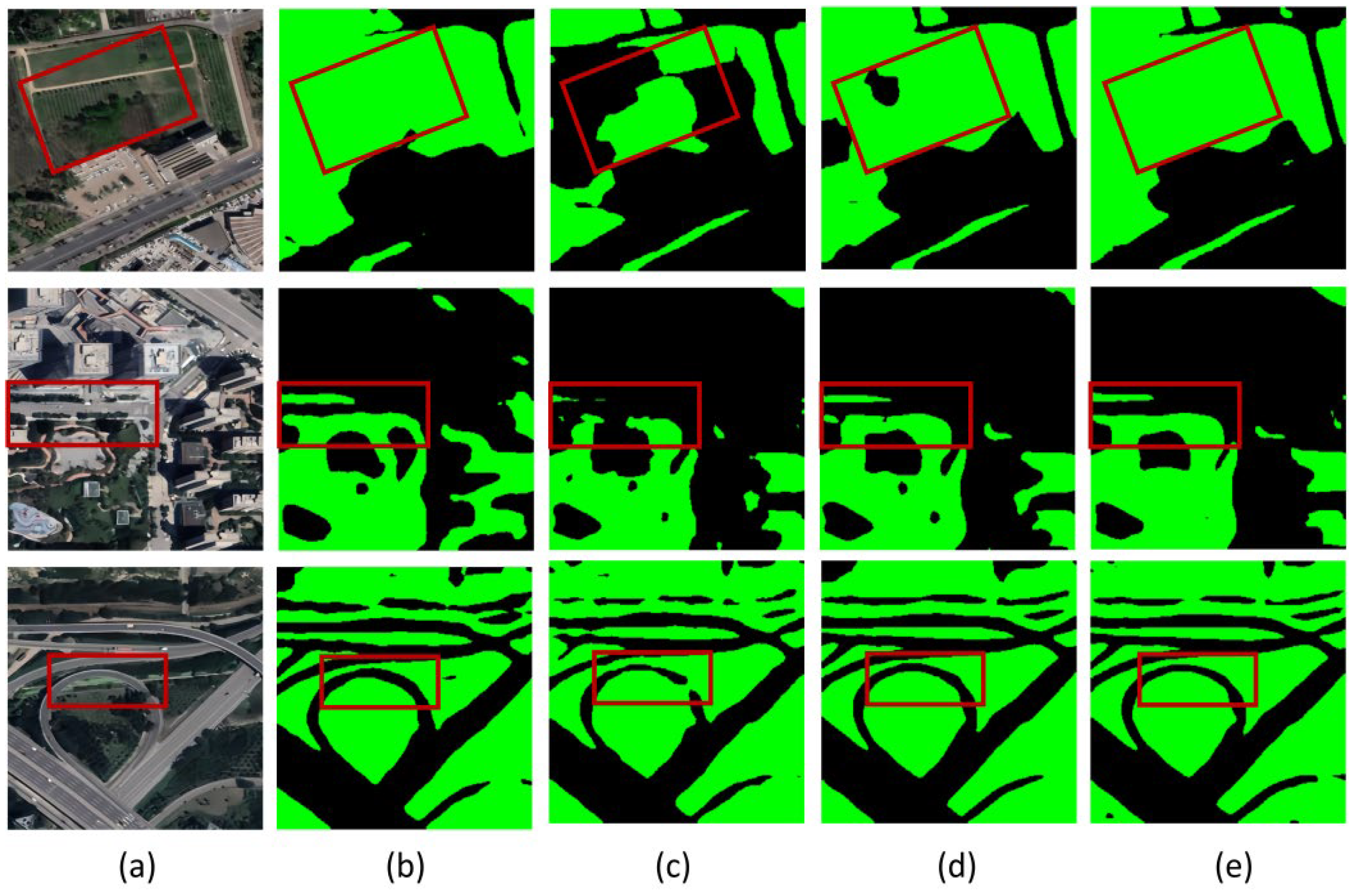
Experimental results for the WHDLD and UGS-1m_Beijing datasets are visualized in Figure 8 and Figure 9, respectively. Segmentation results generated using standard convolutions (Figure 8c and Figure 9c) exhibit noticeable discrepancies compared to the ground truth (Figure 8b and Figure 9b), particularly in boundary localization and the segmentation of irregular shaped regions. As illustrated in the first and fourth rows of Figure 8, standard convolution produces substantial misclassifications at the boundaries between green space and non-green space, frequently misclassifying actual green space as non-green space. In the elongated target regions shown in the second and third rows of Figure 8 and in Figure 9, standard convolution similarly exhibits evident deficiencies. Elongated strip-shaped green spaces are prone to misclassification as non-green space, while elongated roads tend to be misclassified as green space, resulting in jagged distortions and discontinuities along segmentation boundaries. These outputs struggle to match the smooth and regular object contours present in the ground truth images.

In contrast, deformable convolution (Figure 8d and Figure 9d) demonstrates significant advantages. In the first and fourth rows of Figure 8, DConv effectively mitigates the extensive misclassifications between green space and non-green space interfaces. As shown in the second and third rows of Figure 8 and in Figure 9, the segmentation contours produced by DConv closely align with the ground truth, enabling more accurate handling of elongated structures and better preservation of green space details. This improvement stems from DConv’s ability to adaptively adjust its receptive field, thereby modeling irregular green space contours with greater precision.

4.5. Comparison of Different Visible Vegetation Indices as Fourth Input Channel

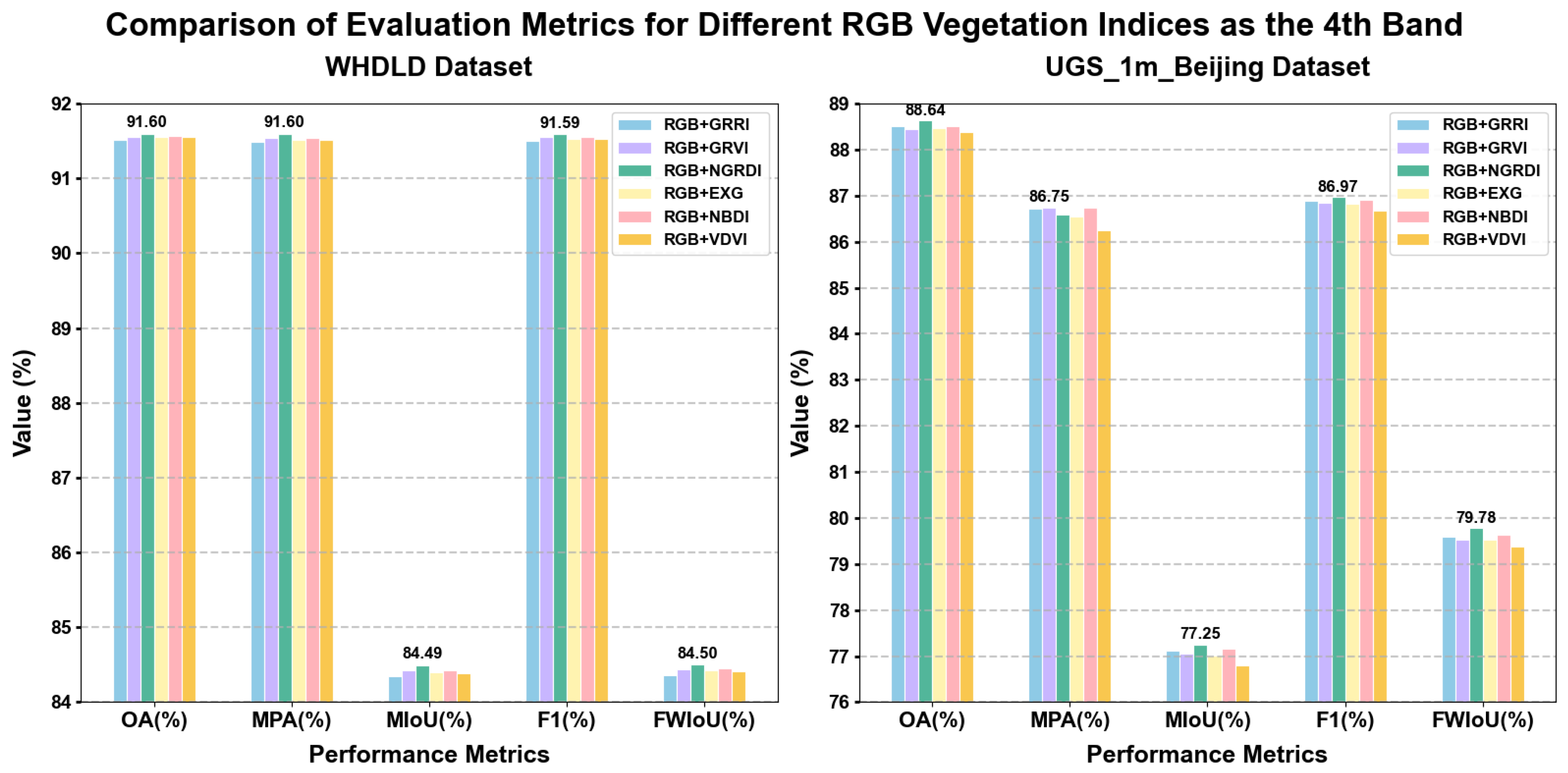
This experiment selected six prominent visible vegetation index (VVI), including EXG, NGRDI, NGBDI, RGRI, GRVI and VDVI, for comparative evaluation. Using the DCNLab model, each VVI was incorporated as a fourth channel alongside the original RGB bands. We assessed the performance on the WHDLD and UGS-1m_Beijing datasets. Descriptions of these VVIs are provided in

Table 3. Definitions and description of the six RGB vegetation indices.

VVI	Formula	Description
Excess Green Index (EXG) [38]	$\mathit{EXG}=2\mathit{G} - \mathit{R} - \mathit{B}$	Enhances the contrast between green vegetation and other features (e.g., soil, water) for vegetation detection.
Normalized Green–Red Difference Index (NGRDI) [39]	$\mathit{NGRDI}={\displaystyle \frac{\mathit{G} - \mathit{R}}{\mathit{G}+\mathit{R}}}$	Highlights vegetation information by utilizing the difference between the green and red bands.
Normalized Green–Blue Difference Index (NGBDI) [40]	$\mathit{NGBDI}={\displaystyle \frac{\mathit{G} - \mathit{B}}{\mathit{G}+\mathit{B}}}$	Reflects vegetation characteristics by calculating the difference between the green and blue bands.
Red–Green Ratio Index (RGRI) [41]	$\mathit{RGRI}={\displaystyle \frac{\mathit{R}}{\mathit{G}}}$	Assesses vegetation health status using the ratio of the red band to the green band.
Green–Red Vegetation Index (GRVI) [42]	$\mathit{GRVI}={\displaystyle \frac{\mathit{R} - \mathit{G}}{\mathit{R}+\mathit{G}}}$	Computes the normalized difference between the green and red bands.
Visible-band Difference Vegetation Index (VDVI) [43]	$\mathit{VDVI}={\displaystyle \frac{2 \times \mathit{G} - \mathit{R} - \mathit{B}}{2 \times \mathit{G}+\mathit{R}+\mathit{B}}}$	Extracts vegetation information using differences in visible bands (e.g., red, green).

, and the corresponding results are illustrated in Figure 10, with detailed numerical values reported in Appendix A 

Table A2. Comparison of Evaluation Metrics Using Different VVIs as the Fourth Band.

Input	WHDLD					UGS-1m_Beijing
	OA (%)	MPA (%)	MIoU (%)	F1 (%)	FWIoU (%)	OA (%)	MPA (%)	MIoU (%)	F1 (%)	FWIoU (%)
RGB + RGRI	91.52	91.49	84.34	91.50	84.36	88.51	86.72	77.12	86.89	79.60
RGB + GRVI	91.56	91.54	84.42	91.55	84.44	88.44	86.75	77.05	86.85	79.52
RGB + NGRDI	91.60	91.60	84.49	91.59	84.50	88.64	86.59	77.25	86.97	79.78
RGB + EXG	91.55	91.51	84.40	91.53	84.42	88.46	86.56	77.01	86.82	79.52
RGB + NGBDI	91.57	91.54	84.43	91.55	84.45	88.52	86.74	77.15	86.91	79.63
RGB + VDVI	91.55	91.51	84.39	91.53	84.41	88.39	86.25	76.79	86.67	79.37

.

According to Figure 10, the performance of models using RGB images combined with different VVIs as a four-channel input was generally comparable across both datasets, with slight differences across various metrics. Among the VVIs, using NGRDI as the fourth channel delivered the best performance across most evaluated metrics. On the WHDLD, the RGB+NGRDI combination outperformed others across all evaluation metrics, achieving an OA of 91.60%, MPA of 91.60%, MIoU of 84.49%, F1-Score of 91.59% and FWIoU of 84.50%. On the UGS-1m_Beijing dataset, although the MPA of RGB + GRVI (86.75%) was slightly higher than that of RGB + NGRDI (86.59%), the RGB + NGRDI combination still maintained its lead in the other evaluation metrics, achieving an OA of 88.64%, MIoU of 77.25%, F1-Score of 86.97% and FWIoU of 79.78%. These results indicate that the normalized green–red difference feature captured by NGRDI provides a stable and effective enhancement when fused with RGB imagery, yielding the strongest synergistic benefits for UGS extraction among the tested indices.

The superior performance of NGRDI can be explained by its underlying physical mechanism. Its calculation formula exploits the unique spectral signature of healthy green vegetation, characterized by strong reflectance in the green band (G) and strong absorption in the red band (R). The numerator (G$-$R) directly amplifies the “greenness” signal of vegetation, while the normalization by the denominator (G + R) effectively mitigates interference from variations in illumination and soil background. In urban environments, many artificial features (e.g., asphalt, concrete, certain construction materials) exhibit relatively similar reflectance in the red and green bands, resulting in NGRDI values close to zero. In contrast, healthy vegetation, characterized by high G and low R values, yields significantly higher positive NGRDI responses. This inherent discriminative power allows NGRDI to more clearly distinguish vegetation from numerous spectrally confounding objects (“different objects with similar spectra”) in complex urban scenes, thereby providing deep learning models with a less noisy and more discriminative spectral prior. Compared to other indices, such as the non-normalized EXG or RGRI which is more sensitive to soil, NGRDI demonstrates superior robustness against complex urban backgrounds. Consequently, NGRDI emerges as the optimal RGB vegetation proxy feature. When its normalized green–red difference information is fused with the original RGB features, it produces the most stable and effective synergistic enhancement.

4.6. Analysis of NGRDI as Fourth Channel and NGRDI Dynamic Weighted Loss

To further explore the depth of utilizing the NGRDI vegetation index, this section, within the DCNLab model framework and on the WHDLD and UGS-1m_Beijing datasets, compares the performance of three strategies: using only the three RGB channels as input, using a four-channel input fusing RGB with NGRDI, and further introducing the NGRDI-based dynamic weighted loss on top of the four-channel input. The experimental results (

Table 4. Comparison of segmentation performance using NGRDI as an additional fourth channel and NGRDI-based Dynamic Weighted Loss.

Method	WHDLD					UGS-1m_Beijing
	OA (%)	MPA (%)	MIoU (%)	F1 (%)	FWIoU (%)	OA (%)	MPA (%)	MIoU (%)	F1 (%)	FWIoU (%)
DCNLab (RGB)	91.13	91.12	83.69	91.12	83.71	88.10	86.00	76.32	86.36	78.92
DCNLab (RGB + NGRDI)	91.60	91.60	84.49	91.59	84.50	88.64	86.59	77.25	86.97	79.78
NGRDI-DCNLab	91.76	91.76	84.77	91.75	84.79	88.68	87.63	77.66	87.27	79.97

) clearly demonstrate that from the RGB input to the introduction of the NGRDI channel, the model’s MIoU significantly improved by approximately 0.8% and 0.93% on the two datasets, respectively. This directly validates the effectiveness of incorporating NGRDI as a spectral prior input for enhancing feature discriminative power.

However, a core innovation of this study lies in applying the same NGRDI prior knowledge simultaneously to the network’s forward propagation (as an input feature) and backward propagation (as a basis for loss weighting), achieving cross-process collaborative optimization. As shown in Table 4, after introducing the NGRDI dynamic weighted loss, the model achieved optimal performance (e.g., MIoU on the WHDLD further increased to 84.77%). In this synergistic mechanism, during forward propagation, NGRDI serves as an input feature providing pixel-level clues about vegetation likelihood to the network. During backward propagation, the weight map calculated based on NGRDI acts as a “supervisor,” automatically identifying difficult areas with ambiguous spectral features and low model prediction confidence (e.g., UGS edges) and assigning them higher weights in the loss calculation. This means the model is not only provided with hints while “seeing” but is also compelled to repeatedly examine and correct those most error-prone parts during its “learning” process.

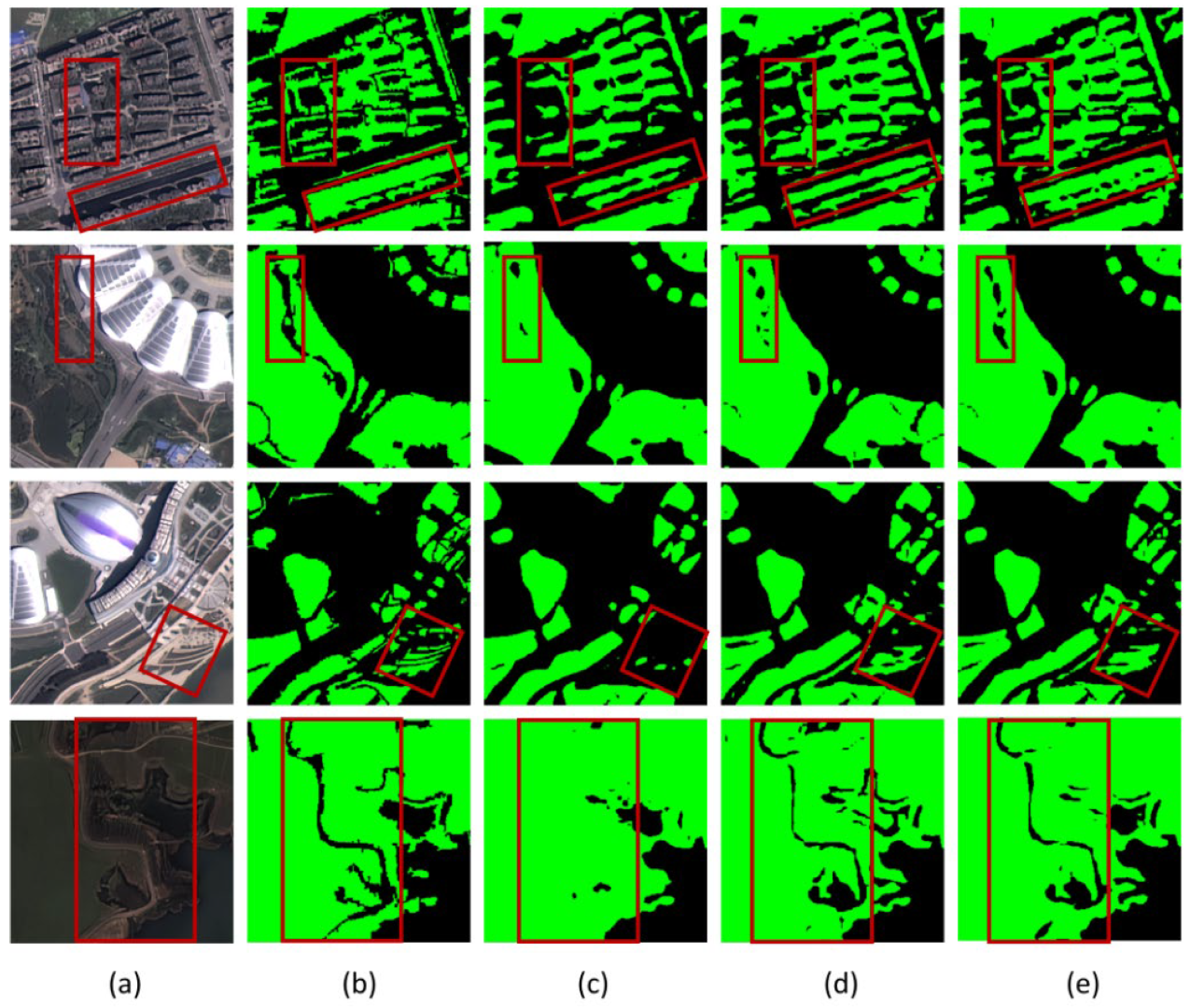
Several example images selected from the WHDLD and UGS-1m_Beijing datasets provide intuitive evidence for this synergistic mechanism, as shown in Figure 11 and Figure 12. As is evident, using only the three RGB channels as input is prone to misjudgment. For instance, as shown in the third row (c) of Figure 11 and the first row (c) of Figure 12, large areas of green space were misclassified as non-green. Furthermore, the fourth row (c) of Figure 11 shows that large non-green areas were misclassified as green space. The introduction of NGRDI as a fourth channel essentially eliminated these misclassifications, enabling correct detection of most UGS. Notably, applying the NGRDI dynamic weighted loss on top of the four-channel RGB + NGRDI input effectively enhanced the extraction of UGS. As illustrated in the first row (e) and second row (e) of Figure 11, and the (e) column of Figure 12, the dynamic weighting process allowed for more precise extraction of UGS. In summary, by employing NGRDI for both feature enhancement and loss weighting, this study constructs a complete utilization loop from feed-forward features to feedback optimization. This deeply exploits the potential of limited spectral priors, significantly enhancing the model’s segmentation accuracy and robustness in complex scenes.

4.7. Application on the UDD6 Dataset

The Urban Drone Dataset 6 (UDD6) dataset is a very high-resolution benchmark for semantic segmentation of remote sensing imagery [44]. It consists of aerial images captured by a DJI Phantom 4 UAV over four different cities in China, at flight altitudes ranging from 60 to 100 m. The original dataset contains six land-cover classes, including vegetation, building facade, road, vehicle, roof and background. For this study, all UAV images and their corresponding label maps were cropped to a standard size of 256 $\times$ 256 pixels. To ensure balanced and representative samples, images with UGS coverage below 30% or above 90% were removed. All non-green categories were merged into a single background class, resulting in a final binary dataset consisting of 5613 images containing only UGS and background, as shown in Figure 13. The dataset was partitioned into training, validation and test sets containing 3929, 842 and 842 image pairs, respectively.

To further verify the generalization ability of our method on ultra-high resolution datasets, we conducted a comparative experiment on the UDD6 UAV dataset, and the results are summarized in

Table 5. Comparison of segmentation performance on the UDD6 Dataset.

Method	OA (%)	MPA (%)	MioU (%)	F1 (%)	FWIoU (%)
Swin-CFNet	92.42	91.55	85.43	92.12	85.83
SegNet	92.54	91.94	85.72	92.29	86.08
PSPNet	92.94	92.35	86.44	92.71	86.78
DABNet	93.32	92.71	87.12	93.10	87.45
Unet++	93.32	92.80	87.14	93.11	87.45
NGRDI-DCNLab	93.50	92.82	87.43	93.27	87.75

. Due to the higher resolution of the drone images and the richer spatial details they contain, the performance improvement of this method compared to the mainstream model Unet++ is limited. The MIoU has only increased by approximately 0.3. However, our method achieved the highest performance across all evaluation metrics on this UAV dataset. In terms of MIoU, it outperformed Swin-CFNet, SegNet, PSPNet, DABNet and UNet++ by 2%, 1.71%, 0.99%, 0.31% and 0.29%, respectively.

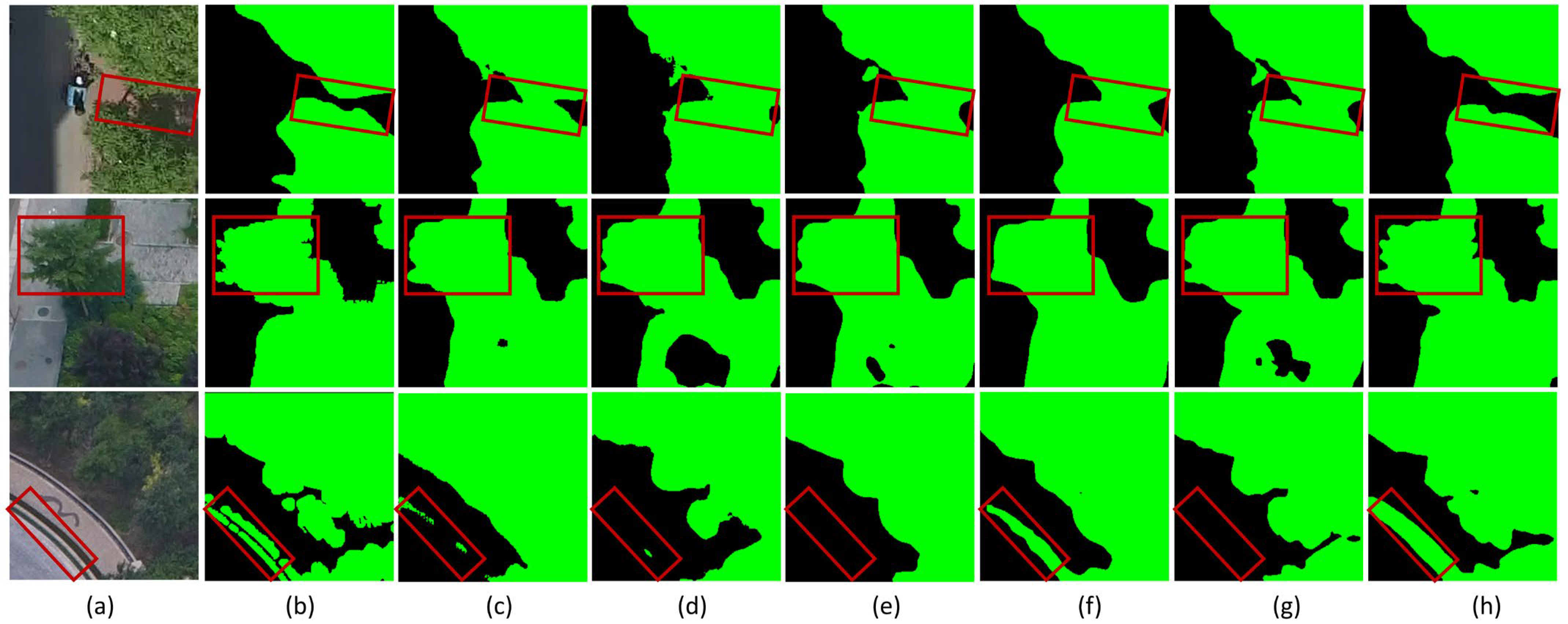
Visual comparisons in Figure 14 further highlight these improvements. In the first row, columns of Figure 14c–h show that models such as SegNet tend to misclassify shadowed regions as green space. By incorporating NGRDI as a fourth channel, the proposed approach effectively mitigates the influence of illumination coefficients, demonstrating superior performance in identifying green space even under shadows and avoiding such misclassification, as evidenced in column (h) of the first row. For irregularly shaped green areas, the feature extraction based on the DConv component enables better contour representation, producing segmentation results that are highly consistent with the ground truth in morphology, as shown in column (h) of the second row. Furthermore, the proposed method demonstrates strong capability in detecting small, fragmented green patches, reducing missed detections and enhancing segmentation completeness, as illustrated in column (h) of the third row. Therefore, these results demonstrate that the proposed method is effective and possesses certain generalization capability for UGS extraction on the UDD6 UAV dataset.

5. Discussion

This study addresses the dual challenges of spectral confusion and blurred geometric boundaries in UGS extraction using only RGB imagery. Existing methods typically rely on NIR bands [1,13,14] or more complex network architectures [1,12,13,14,15,16], which exhibit significant limitations in terms of data source universality. Moreover, they often fail to specifically optimize for the inherent difficulty in RGB imagery: the relatively weak spectral signature of vegetation and its susceptibility to confusion with artificial features. Confronted by these challenges, our work introduces the NGRDI-DCNLab model. Its innovation lies not merely in incremental adjustments but in a fundamental shift towards a coherent optimization system that orchestrates the entire workflow, from input through feature representation to objective optimization, thereby ensuring a systematic response to the complex problems identified. The core of this system lies in the coordinated design of feature enhancement, structure adaptation and optimization guidance. Firstly, the NGRDI is introduced as an input channel, injecting a physically interpretable spectral prior for vegetation into the model to mitigate spectral confusion at the source [45]. Secondly, deformable convolution is employed in the decoder [46], enabling the network to adaptively conform to the irregular contours of green spaces, thereby achieving refined boundary modeling. Most critically, the proposed NGRDI-weighted loss function deeply integrates the same spectral prior into the optimization process, actively focusing the model on hard-to-separate samples to drive targeted learning. These three modules form a closed-loop, ensuring the deep exploitation and effective utilization of the limited spectral information.

To validate the advantages of our synergistic framework under the “RGB-only” condition, we conducted systematic experimental comparisons. On both the WHDLD and UDD6 datasets, the performance of NGRDI-DCNLab stably surpassed a series of mainstream segmentation models, including PSPNet, DABNet, SegNet, and U-Net++. For instance, on the WHDLD, our model achieved an mIoU of 84.77%, which is significantly superior to the best-performing baseline model, U-Net++ (83.99%). These results demonstrate that a synergistic design targeting specific bottlenecks can more effectively unleash performance potential under limited data conditions than directly applying or fine-tuning generic architectures. Compared to recent advanced models also developed for UGS extraction (e.g., STRD-Net [1], MFFTNet [13]), our study completely abandons reliance on the NIR band. It explores a new pathway to achieve high accuracy under pure RGB conditions through spectral, spatial and optimization synergy, thereby establishing a more universal and high-performance benchmark for such tasks.

The proposed method eliminates the reliance on NIR data, offering significant practical value. It enables large-scale, high-frequency, and fine-grained monitoring of UGS using low-cost, readily available RGB data sources such as consumer-grade drones and open-source satellite imagery. This significantly lowers the technical application threshold and cost, providing an efficient and reliable tool for urban ecological assessment, planning management, and research [47]. However, this study also has certain limitations. The performance of the proposed model varies across different spatial scales. On the WHDLD satellite image dataset (with a spatial resolution of 2 m), the proposed method significantly outperforms mainstream segmentation models, demonstrating its superiority on moderately high-resolution imagery. However, on the ultra-high-resolution UAV dataset UDD6, although the model exhibits some generalization benefit, its capacity is constrained due to the richer spatial details contained in UAV imagery. Therefore, the proposed method is more suitable for urban green space extraction from moderately high-resolution RGB satellite images. For higher-resolution UAV imagery, future work could consider fine-tuning the approach based on the specific characteristics of UAV data. Meanwhile, the model’s performance has currently been validated primarily in urban scenes during the growing season. The spectral and morphological characteristics of vegetation undergo significant changes with phenological seasons (e.g., autumn coloration) and across geographical environments (e.g., farmland, forests), posing a potential challenge to its generalizability [48]. Future work necessitates the construction of annotated datasets encompassing multi-temporal and multi-regional scenes, and the exploration of strategies such as domain adaptation to further enhance the model’s robustness and applicability across complex and variable real-world scenarios.

6. Conclusions

The NGRDI-DCNLab model proposed in this paper systematically addresses three major bottlenecks in UGS extraction relying solely on RGB imagery. First, to tackle the weak discriminative power of vegetation spectral features caused by the absence of a NIR band in RGB data, the model introduces the NGRDI to construct a four-channel input. This injects an explicit spectral prior for vegetation into the model, effectively compensating for the missing key information and thereby enhancing the spectral separability between vegetation and non-vegetation features. Second, confronting the challenge of blurred segmentation boundaries due to the irregular morphology of UGS, the model employs deformable convolutions to refine the decoder, significantly improving its ability to dynamically fit and delineate complex contours. Finally, to ameliorate the model’s insufficient learning on hard samples such as spectrally confused areas, a novel NGRDI-based dynamic weighted loss function is designed. This mechanism adaptively focuses on difficult-to-classify pixels and ambiguous boundaries, driving the model to optimize its segmentation strategy. Experimental results demonstrate that through these coordinated improvements, the model achieves superior extraction accuracy and clearer boundary details on three RGB-only datasets—WHDLD, UGS-1m_Beijing, and UDD6—fully validating the effectiveness and practical utility of this method as a high-precision, low-cost technical solution.

References

1. Yu, M.; He, L.; Shen, Z.; Lv, M. STRD-Net: A Dual-Encoder Semantic Segmentation Network for Urban Green Space Extraction. IEEE Trans. Geosci. Remote Sens. 2024, 62, 1–13. [Google Scholar] [CrossRef]
2. Wang, T.; Hu, H. Mapping Urban Heat Island Networks Using a Landscape Connectivity Approach: A Case Study of Nanjing. Sustain. Cities Soc. 2025, 132, 106800. [Google Scholar] [CrossRef]
3. Zhi, J.; Ge, L.; Geng, T.; Zhang, Z.; Li, L.; Zhu, H.; Zhou, Z.; Jiang, W.; Qu, L.; Su, Y.; et al. Accurately Mapping Social Functional Zones of Urban Green Spaces by Integrating Remote Sensing Images and Crowd-Sourced Geospatial Data. Int. J. Digit. Earth 2024, 17, 1–26. [Google Scholar] [CrossRef]
4. Lobert, F.; Schwieder, M.; Alsleben, J.; Broeg, T.; Kowalski, K.; Okujeni, A.; Hostert, P.; Erasmi, S. Unveiling Year-Round Cropland Cover by Soil-Specific Spectral Unmixing of Landsat and Sentinel-2 Time Series. Remote Sens. Environ. 2025, 318, 114594. [Google Scholar] [CrossRef]
5. Hu, Z.; Chu, Y.; Zhang, Y.; Zheng, X.; Wang, J.; Xu, W.; Wang, J.; Wu, G. Scale Matters: How Spatial Resolution Impacts Remote Sensing Based Urban Green Space Mapping? Int. J. Appl. Earth Obs. Geoinf. 2024, 134, 104178. [Google Scholar] [CrossRef]
6. Vizzari, M.; Antonielli, F.; Bonciarelli, L.; Grohmann, D.; Menconi, M.E. Urban Greenery Mapping Using Object-Based Classification and Multi-Sensor Data Fusion in Google Earth Engine. Urban For. Urban Green. 2025, 105, 128697. [Google Scholar] [CrossRef]
7. Chen, B.; Zhang, Q.; Yang, N.; Wang, X.; Zhang, X.; Chen, Y.; Wang, S. Deep Learning Extraction of Tidal Creeks in the Yellow River Delta Using GF-2 Imagery. Remote Sens. 2025, 17, 676. [Google Scholar] [CrossRef]
8. Ronneberger, O.; Fischer, P.; Brox, T. U-Net: Convolutional Networks for Biomedical Image Segmentation. In International Conference on Medical Image Computing and Computer-Assisted Intervention; Springer: Cham, Switzerland, 2015; pp. 234–241. [Google Scholar]
9. Zhao, H.; Shi, J.; Qi, X.; Wang, X.; Jia, J. Pyramid Scene Parsing Network. In Proceedings of the IEEE Conference on Computer Vision and Pattern Recognition (CVPR), Honolulu, HI, USA, 21–26 July 2017. [Google Scholar]
10. Chen, L.-C.; Zhu, Y.; Papandreou, G.; Schroff, F.; Adam, H. Encoder-Decoder with Atrous Separable Convolution for Semantic Image Segmentation. In Computer Vision—ECCV 2018; Ferrari, V., Hebert, M., Sminchisescu, C., Weiss, Y., Eds.; Lecture Notes in Computer Science; Springer International Publishing: Cham, Switzerland, 2018; Volume 11211, pp. 833–851. ISBN 978-3-030-01233-5. [Google Scholar]
11. Badrinarayanan, V.; Kendall, A.; Cipolla, R. SegNet: A Deep Convolutional Encoder-Decoder Architecture for Image Segmentation. IEEE Trans. Pattern Anal. Mach. Intell. 2017, 39, 2481–2495. [Google Scholar] [CrossRef]
12. Yu, K.; Biao, W.; Yanglan, W.U.; Botao, C.; Xingdi, C.; Weibao, X.U.E. Urban Vegetation Classification Based on Multi-Scale Feature Perception Network for UAV Images. J. Geo-Inf. Sci. 2022, 24, 962–980. [Google Scholar] [CrossRef]
13. Cheng, Y.; Wang, W.; Ren, Z.; Zhao, Y.; Liao, Y.; Ge, Y.; Wang, J.; He, J.; Gu, Y.; Wang, Y.; et al. Multi-Scale Feature Fusion and Transformer Network for Urban Green Space Segmentation from High-Resolution Remote Sensing Images. Int. J. Appl. Earth Obs. Geoinf. 2023, 124, 103514. [Google Scholar] [CrossRef]
14. Wang, W.; Cheng, Y.; Ren, Z.; He, J.; Zhao, Y.; Wang, J.; Zhang, W. A Novel Hybrid Method for Urban Green Space Segmentation from High-Resolution Remote Sensing Images. Remote Sens. 2023, 15, 5472. [Google Scholar] [CrossRef]
15. Wu, Y.; Zhang, M. Swin-CFNet: An Attempt at Fine-Grained Urban Green Space Classification Using Swin Transformer and Convolutional Neural Network. IEEE Geosci. Remote Sens. Lett. 2024, 21, 1–5. [Google Scholar] [CrossRef]
16. Chen, K.; Wang, Y.; Huang, C.; Wang, J.; Li, S.L.; Guan, H.; Ma, L. GreenNet: A Dual-Encoder Network for Urban Green Space Classification Using High-Resolution Remotely Sensed Images. Int. J. Appl. Earth Obs. Geoinf. 2025, 142, 104709. [Google Scholar] [CrossRef]
17. Zhang, Z.; Hu, Q.; Fang, H.; Liu, W.; Feng, R.; Chen, S.; Wu, Q.; Wang, P.; Lu, W. TriGEFNet: A Tri-Stream Multimodal Enhanced Fusion Network for Landslide Segmentation from Remote Sensing Imagery. Remote Sens. 2026, 18, 186. [Google Scholar] [CrossRef]
18. Lee, J.; Shin, J.; Lee, S.; Chun, C.-J. LSR-Net: A Lightweight and Strong Robustness Network for Bearing Fault Diagnosis in Noise Environment. arXiv 2026, arXiv:2601.10761. [Google Scholar] [CrossRef]
19. Li, R.; Zheng, S.; Duan, C.; Wang, L.; Zhang, C. Land Cover Classification from Remote Sensing Images Based on Multi-Scale Fully Convolutional Network. Geo-Spat. Inf. Sci. 2022, 25, 278–294. [Google Scholar] [CrossRef]
20. Shi, Q.; Liu, M.; Marinoni, A.; Liu, X. UGS-1m: Fine-Grained Urban Green Space Mapping of 31 Major Cities in China Based on the Deep Learning Framework. Earth Syst. Sci. Data 2023, 15, 555–577. [Google Scholar] [CrossRef]
21. Lei, T.; Xu, Y.; Ning, H.; Lv, Z.; Min, C.; Jin, Y.; Nandi, A.K. Lightweight Structure-Aware Transformer Network for Remote Sensing Image Change Detection. IEEE Geosci. Remote Sens. Lett. 2024, 21, 1–5. [Google Scholar] [CrossRef]
22. Saponaro, M.; Agapiou, A.; Hadjimitsis, D.G.; Tarantino, E. Influence of Spatial Resolution for Vegetation Indices’ Extraction Using Visible Bands from Unmanned Aerial Vehicles’ Orthomosaics Datasets. Remote Sens. 2021, 13, 3238. [Google Scholar] [CrossRef]
23. Khuimphukhieo, I.; Chavez, J.C.; Yang, C.; Pasupuleti, L.A.; Olaniyi, I.; Ancona, V.; Mandadi, K.K.; Jung, J.; Enciso, J. Assessing Huanglongbing Severity and Canopy Parameters of the Huanglongbing-Affected Citrus in Texas Using Unmanned Aerial System-Based Remote Sensing and Machine Learning. Sensors 2024, 24, 7646. [Google Scholar] [CrossRef]
24. Li, Z.; Liu, F.; Yang, W.; Peng, S.; Zhou, J. A Survey of Convolutional Neural Networks: Analysis, Applications, and Prospects. IEEE Trans. Neural Netw. Learn. Syst. 2022, 33, 6999–7019. [Google Scholar] [CrossRef]
25. Sajadi, P.; Gholamnia, M.; Bonafoni, S.; Mills, G.; Sang, Y.-F.; Li, Z.; Khan, S.; Han, J.; Pilla, F. Automated Pixel Purification for Delineating Pervious and Impervious Surfaces in a City Using Advanced Hyperspectral Imagery Techniques. IEEE Access 2024, 12, 82560–82583. [Google Scholar] [CrossRef]
26. Wei, X.-S.; Song, Y.-Z.; Aodha, O.M.; Wu, J.; Peng, Y.; Tang, J.; Yang, J.; Belongie, S. Fine-Grained Image Analysis with Deep Learning: A Survey. IEEE Trans. Pattern Anal. Mach. Intell. 2022, 44, 8927–8948. [Google Scholar] [CrossRef]
27. Lian, X.; Pang, Y.; Han, J.; Pan, J. Cascaded Hierarchical Atrous Spatial Pyramid Pooling Module for Semantic Segmentation. Pattern Recognit. 2021, 110, 107622. [Google Scholar] [CrossRef]
28. Li, Y.; Liu, S.; Wu, J.; Sun, W.; Wen, Q.; Wu, Y.; Qin, X.; Qiao, Y. Multi-Scale Kolmogorov-Arnold Network (KAN)-Based Linear Attention Network: Multi-Scale Feature Fusion with KAN and Deformable Convolution for Urban Scene Image Semantic Segmentation. Remote Sens. 2025, 17, 802. [Google Scholar] [CrossRef]
29. Dong, W.; Zhou, C.; Wu, F.; Wu, J.; Shi, G.; Li, X. Model-Guided Deep Hyperspectral Image Super-Resolution. IEEE Trans. Image Process. 2021, 30, 5754–5768. [Google Scholar] [CrossRef]
30. Zhou, T.; Wang, W. Cross-Image Pixel Contrasting for Semantic Segmentation. IEEE Trans. Pattern Anal. Mach. Intell. 2024, 46, 5398–5412. [Google Scholar] [CrossRef]
31. Wang, X.; Chen, Y.; Zhu, W. A Survey on Curriculum Learning. IEEE Trans. Pattern Anal. Mach. Intell. 2022, 44, 4555–4576. [Google Scholar] [CrossRef]
32. Abdullah, S.S.; Rajasekaran, M.P. Automatic Detection and Classification of Knee Osteoarthritis Using Deep Learning Approach. Radiol. Med. 2022, 127, 398–406. [Google Scholar] [CrossRef]
33. Albattah, W.; Khan, R.U. Impact of Imbalanced Features on Large Datasets. Front. Big Data 2025, 8, 1455442. [Google Scholar] [CrossRef]
34. Kim, J.; Lee, Y.-K.; Choi, C.-S.; Fereshtenejad, S.; Song, J.-J. Scanline Intersection Similarity: A Similarity Metric for Joint Trace Maps. Comput. Geosci. 2023, 175, 105358. [Google Scholar] [CrossRef]
35. Maxwell, A.E.; Warner, T.A.; Guillén, L.A. Accuracy Assessment in Convolutional Neural Network-Based Deep Learning Remote Sensing Studies—Part 1: Literature Review. Remote Sens. 2021, 13, 2450. [Google Scholar] [CrossRef]
36. Zhao, H.; Luo, P.; Cui, W.; Xia, C.; Xu, X.; Feng, Z.; Chen, J.; Wang, J.; Xun, W.; Chen, C. Geographical Scenario Knowledge-Informed Graph Structure Attention for Image Segmentation. IEEE Trans. Geosci. Remote Sens. 2025, 63, 1–16. [Google Scholar] [CrossRef]
37. Cheng, B.; Girshick, R.; Dollar, P.; Berg, A.C.; Kirillov, A. Boundary IoU: Improving Object-Centric Image Segmentation Evaluation. In Proceedings of the 2021 IEEE/CVF Conference on Computer Vision and Pattern Recognition (CVPR), Nashville, TN, USA, 20–25 June 2021; IEEE: Nashville, TN, USA, 2021; pp. 15329–15337. [Google Scholar]
38. Ye, X.; Zhu, W.; Liu, R.; He, B.; Yang, X.; Zhao, C. An Automated Method for Estimating Fractional Vegetation Cover from Camera-Based Field Measurements: Saturation-Adaptive Threshold for ExG (SATE). ISPRS J. Photogramm. Remote Sens. 2025, 229, 170–187. [Google Scholar] [CrossRef]
39. Macedo, F.L.; Nóbrega, H.; De Freitas, J.G.R.; Pinheiro De Carvalho, M.A.A. Assessment of Vegetation Indices Derived from UAV Imagery for Weed Detection in Vineyards. Remote Sens. 2025, 17, 1899. [Google Scholar] [CrossRef]
40. Lyu, H.; Grafton, M.; Ramilan, T.; Irwin, M.; Wei, H.-E.; Sandoval, E. Using Remote and Proximal Sensing Data and Vine Vigor Parameters for Non-Destructive and Rapid Prediction of Grape Quality. Remote Sens. 2023, 15, 5412. [Google Scholar] [CrossRef]
41. Huang, J.; Lu, X.; Chen, L.; Sun, H.; Wang, S.; Fang, G. Accurate Identification of Pine Wood Nematode Disease with a Deep Convolution Neural Network. Remote Sens. 2022, 14, 913. [Google Scholar] [CrossRef]
42. Zhu, L.; Liu, X.; Wang, Z.; Tian, L. High-Precision Sugarcane Yield Prediction by Integrating 10-m Sentinel-1 VOD and Sentinel-2 GRVI Indexes. Eur. J. Agron. 2023, 149, 126889. [Google Scholar] [CrossRef]
43. Yang, A.; Wang, C.; Yang, Q.; Pang, G.; Long, Y.; Wang, L.; Yang, L.; Cruse, R.M. Choosing the Right Horizontal Resolution for Gully Erosion Susceptibility Mapping Using Machine Learning Algorithms: A Case in Highly Complex Terrain. Remote Sens. 2022, 14, 2580. [Google Scholar] [CrossRef]
44. Sun, Y.; Shao, Z.; Cheng, G.; Huang, X.; Wang, Z. Road and Car Extraction Using UAV Images via Efficient Dual Contextual Parsing Network. IEEE Trans. Geosci. Remote Sens. 2022, 60, 1–13. [Google Scholar] [CrossRef]
45. Jansone, Z.; Bleidere, M.; Putniece, G. Estimating spring wheat nitrogen use efficiency via proximal and UAV sensing in Northwest Latvia. Agron. Res. 2026, 24, xxx–ccc. [Google Scholar]
46. Gautam, A.; Pawar, A.; Joshi, A.; Tazi, S.N.; Chaudhary, S.; Hambadre, P.; Dudhane, A.; Vipparthi, S.K.; Murala, S. Pureformer: Transformer-Based Image Denoising. In Proceedings of the 2025 IEEE/CVF Conference on Computer Vision and Pattern Recognition Workshops (CVPRW), Nashville, TN, USA, 11–12 June 2025; pp. 1–9. [Google Scholar]
47. Woodruff, C.D.; Clark, P.E.; Olsoy, P.J.; Enterkine, J. Estimation of Leaf Area Index in Sagebrush Steppe with Low Cost Unoccupied Aerial Systems. Landsc. Ecol. 2025, 40, 27. [Google Scholar] [CrossRef]
48. Small, C.; Sousa, D. Spectroscopic Phenological Characterization of Mangrove Communities. Remote Sens. 2024, 16, 2796. [Google Scholar] [CrossRef]
Figure 1. Example samples from the WHDLD. (a) High-resolution remote sensing images; (b) original multi-class annotations; (c) urban green space labels used in this study.
Land 15 00486 g001
Figure 2. Representative samples from the UGS-1m_Beijing dataset. (a) High-resolution remote sensing images; (b) corresponding urban green space labels used in this study.
Land 15 00486 g002
Figure 3. Architecture of the NGRDI-DCNLab model. W M represents the spectral weight map; L o s s denotes the overall loss; l o s s p refers to the pixel-wise binary cross-entropy loss.
Land 15 00486 g003
Figure 4. Schematic diagram of sampling locations. (a) Standard convolution; (b) deformable convolution.
Land 15 00486 g004
Figure 5. The distribution of green and non-green NGRDI values for the WHDLD and UGS-1m_Beijing datasets. (a) the distribution of green and non-green NGRDI values in the WHDLD dataset; (b) the distribution of green and non-green NGRDI values in the UGS-1m_Beijing dataset; (c) the distribution of NGRDI values in the WHDLD dataset after green and non-green processing; (d) the distrubution of NGRDI values in the UGS-1m_Beijing dataset after green and non-green processing.
Land 15 00486 g005
Figure 6. Comparison of evaluation indicators for the different models.
Land 15 00486 g006
Figure 7. Comparison of urban green space segmentation results obtained by different models. (a) Original image; (b) Ground truth; (c) PSPNet; (d) DABNet; (e) SegNet; (f) Swin-CFNet; (g) Unet++; (h) DCNLab.
Land 15 00486 g007
Figure 8. Comparison of segmentation results on the WHDLD. (a) Original image; (b) ground truth; (c) standard 3 × 3 convolution; (d) deformable convolution (DConv).
Land 15 00486 g008
Figure 9. Comparison of segmentation results on the UGS-1m_Beijing Dataset. (a) original image; (b) ground truth; (c) standard 3 × 3 convolution; (d) deformable convolution (DConv).
Land 15 00486 g009
Figure 10. Comparison of evaluation metrics using different VVIs as the fourth input channel.
Land 15 00486 g010
Figure 11. Comparison of segmentation results on the WHDLD. (a) Original image; (b) ground truth; (c) RGB three-channel input; (d) RGB+NGRDI four-channel input; (e) NGRDI-DCNLab.
Land 15 00486 g011
Figure 12. Comparison of segmentation results on the UGS-1m_Beijing dataset. (a) Original image; (b) ground truth; (c) RGB three-channel input; (d) RGB + NGRDI four-channel input; (e) NGRDI-DCNLab.
Land 15 00486 g012
Figure 13. Sample from the UDD6 dataset. (a) UAV image; (b) multi-class labels; (c) urban green space label.
Land 15 00486 g013
Figure 14. Comparison of segmentation results by different models on the UDD6 dataset. (a) Original image; (b) ground truth; (c) Swin-CFNet; (d) SegNet; (e) PSPNet; (f) DABNet; (g) UNet++; (h) NGRDI-DCNLab.
Land 15 00486 g014