The Data-Driven System Dynamics Study on Sustainable Development of Urban Ecosystems: Causal Discovery and Simulation Analysis in Yangtze River Delta

Abstract

The urban ecosystem constitutes a complex adaptive system comprising interdependent subsystems—environment, population, infrastructure, public services, environmental governance, and socio-economic factors. Conventional system dynamics (SD) modeling relies on expert-derived causal assumptions, which have limitations in objectivity, transferability, and adaptability. To solve these, this study develops a data-driven SD modeling framework that infers causal structures from time-series data of 38 sustainability indicators. The framework integrates multiple causal inference techniques to identify causal relationships among variables, then systematically identifies stock variables and constructs an SD simulation model. Applying it to panel data from 41 cities in China’s Yangtze River Delta (2013–2022), the study characterizes the causal network topology, interaction patterns between subsystems, dominant feedback loops, and temporal evolution trajectories of key stock variables. Results show: (1) There is significant cross-city variation in causal network structure due to differences in urban development and institutional configurations; (2) Environmental conditions are the most frequently affected terminal node with an average normalized causal strength of 0.277, higher than other subsystems; (3) Several cross-subsystem positive and negative feedback loops are identified, highlighting potential path dependencies and intervention-sensitive nodes for sustainable urban transitions. This study provides a replicable, comparable, and scalable framework for urban sustainable development analysis, offering data-driven support for smart city management and policy formulation.

1. Introduction

Against the backdrop of accelerated urbanization and tightening ecological constraints, sustainable urban development has emerged as a crucial issue in contemporary regional governance and academic research [1,2]. As a fundamental pillar of economic growth and urban planning, urban systems represent complex adaptive systems comprising social, economic, environmental, and governance subsystems. These subsystems interact through nonlinear relationships, time lags, and feedback loops, collectively governing the dynamic evolution of urban sustainable development [3,4,5,6]. As the world’s second-largest economy, China’s urbanization process is unprecedented in both scale and speed, making its exploration and practice in sustainable urban development highly representative and exemplary on the global stage. China’s experience in balancing urban economic growth, social progress, and environmental protection not only provides valuable lessons for developing countries undergoing rapid urbanization but also offers insights for developed nations seeking to achieve more sustainable urban forms. The Yangtze River Delta urban agglomeration, being one of China’s most economically dynamic and highly urbanized regions, demonstrates sustainable development pathways and operational principles that have significant demonstrative value for high-quality development across the nation and similar urban clusters. Current research on urban sustainable development has primarily concentrated on establishing static evaluation systems and quantifying coupling coordination degrees [7,8,9]. Although these approaches can reveal the status and overall performance of systems, they are unable to accurately capture the intrinsic causal relationships and dynamic evolution processes among elements. Traditional System Dynamics (SD) models, although effective in capturing the dynamic behaviors of complex systems, rely excessively on the subjective judgments of domain experts when specifying causal relationships among variables [10,11]. This dependence on human bias often undermines the empirical validity and generalizability of the models. Moreover, existing studies tend to focus on city-specific analyses at the individual city scale, while systematic cross-regional comparisons of the structural configurations and operational mechanisms of sustainable development systems within and across urban agglomerations remain insufficient [12,13,14,15]. As a result, they fail to discover the common characteristics and heterogeneous patterns in regional urban development.

To address these limitations, this study aims to investigate the causal structural configurations and dynamic operational mechanisms of urban sustainable development systems within the Yangtze River Delta urban agglomeration [16,17,18,19]. Specifically, it seeks to answer the following research questions: First, what are the key causal relationships and feedback loops that drive the dynamic evolution of sustainable development in cities within the Yangtze River Delta? Second, how do these causal structures and feedback mechanisms vary across different cities, and can distinct urban types be identified based on their causal similarity? Third, what are the common characteristics and heterogeneous patterns in the sustainable development systems of these cities, and what policy implications do these findings hold for regional high-quality development? By addressing these questions, this research endeavors to bridge the gap between static evaluation and dynamic mechanism analysis, reduce the subjectivity in SD model construction, and provide a deeper understanding of the complex interplay within urban sustainable development systems. The goal is to offer theoretical support and practical guidance for formulating targeted and regionally adaptive sustainable development strategies in the Yangtze River Delta and beyond [20].

To tackle the challenges, this study chose 41 core cities in the Yangtze River Delta region as research objects and collected panel data from 2013 to 2022. A comprehensive evaluation system was established, incorporating six subsystems, namely environmental pressure, environmental level, population and infrastructure, public utilities, environmental governance, and socio-economic development, which consisted of 38 core indicators. Environmental pressure was set as a control variable-based subsystem, and a data-driven system dynamics analysis method for urban sustainable development was put forward. Building on traditional system dynamics (SD) modeling, this method integrates three empirical methods: lag correlation analysis, Lasso regression variable screening, and Granger causality testing. It identifies statistically significant causal relationships and relative influence intensities among indicators from observational data. Based on these results, a data-supported SD structural model was constructed to identify key feedback loops within the system, quantify their gain coefficients, and determine their polarity (positive/negative feedback). Finally, dynamic evolution simulations were carried out for core stock variables (e.g., Gross Domestic Product, GDP).

This study carried out exploratory work in three key areas: First, multi-method causal inference (combining lagged correlation analysis and Lasso regression) was integrated with system dynamics modeling processes to establish a coherent framework for the transition from observational data to system dynamics models. This approach obviates the necessity for manual structural assumptions. Initial causal relationships are generated through data-driven methods, and simulation models are subsequently constructed. Second, 38 indicators covering six subsystems—environmental pressure, environmental conditions (level), population and infrastructure, public utilities, environmental governance, and socio-economic subsystem—were selected to characterize the multidimensional features of urban ecosystems. The selection of indicators was based on the availability and continuity of publicly accessible statistical data, avoiding restrictions to single domains or specific policy dimensions. Third, comparative analysis was performed via cross-city comparisons to examine the similarities and differences in the results of causal structure identification and the trajectory evolution of existing variables across cities. This design does not pre-assume specific development models. Instead, structural variations and dynamic pathways are presented side by side to facilitate the identification of potential common patterns and differentiated characteristics.

The structure of this paper is organized as follows: Section 2 outlines the materials, including indicator definitions and data sources at the data level. Section 3 outlines methodology, including causal inference procedures at the methodological level, system dynamics modeling logic at the model level, and cross-city comparison operations at the application level. Section 4 presents empirical findings, encompassing identified causal relationships across cities, interaction patterns between subsystems, feedback loop identification results, temporal trends of major stock variables, and intercity comparisons. Section 5 clarifies the study’s applicability boundaries and policy implications. Section 6 concludes the paper with a summary. Section 7 outlines the limitations and future studies.

2. Materials

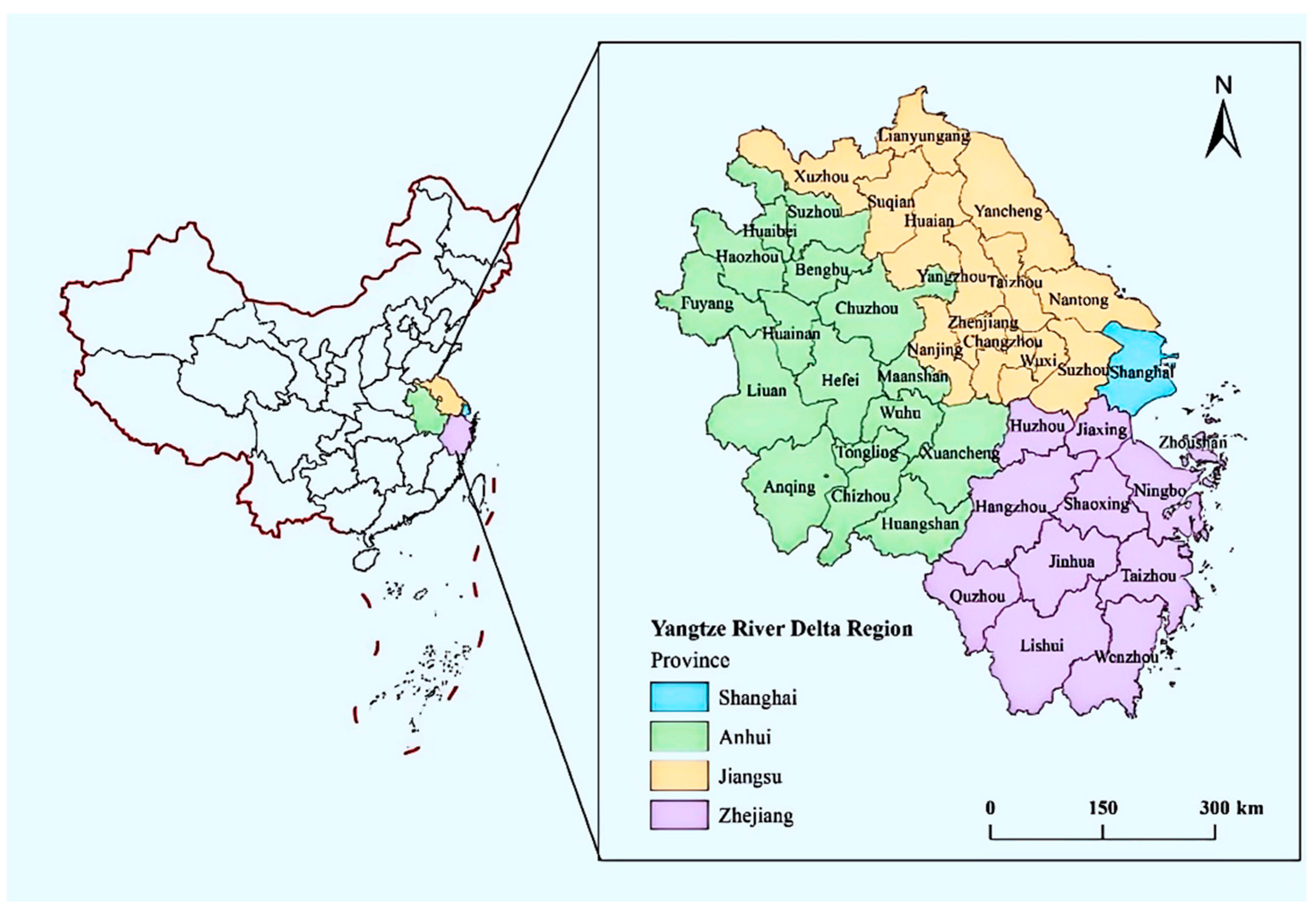
The Yangtze River Delta (hereinafter referred to as “Yangtze River Delta”) is in the eastern coastal area of China, situated in the lower reaches of the Yangtze River, bordering the Yellow Sea and the East China Sea. Its geographical coordinates are east longitude 114°54′–123°10′, north latitude 27°02′–35°20′. The study area covers Shanghai, 13 prefecture-level cities in Jiangsu Province, 11 prefecture-level cities in Zhejiang Province, and 16 prefecture-level cities in Anhui Province, totaling 41 cities at or above the prefecture level (

Table 1. List of 41 prefecture-level cities in the Yangtze River Delta urban agglomeration.

Province/Municipality	Cities
Shanghai Municipality	Shanghai
Jiangsu Province	Nanjing, Wuxi, Xuzhou, Changzhou, Suzhou, Nantong, Lianyungang, Huai’an, Yancheng, Yangzhou, Zhenjiang, Taizhou, Suqian
Zhejiang Province	Hangzhou, Ningbo, Wenzhou, Jiaxing, Huzhou, Shaoxing, Jinhua, Quzhou, Zhoushan, Taizhou, Lishui
Anhui Province	Hefei, Wuhu, Bengbu, Huainan, Ma’anshan, Huaibei, Tongling, Anqing, Huangshan, Chuzhou, Fuyang, Suzhou, Lu’an, Bozhou, Chizhou, Xuancheng

, Figure 1).

Based on the urban ecosystem theory [21] and the monitoring indicator system for the United Nations Sustainable Development Goals [22], this study established a six-dimensional evaluation system for urban sustainable development, which encompasses 38 indicators, as shown in

Table 2. Major categories and sub-indicators of the urban sustainable development index system.

Subsystem	Index	Index Code
Environment Pressure (EP)	Number of days with high temperature (days)	X1
	Number of days with low temperature (days)	X2
	Number of days with heavy rain (days)	X3
	Number of days with strong wind or above (days)	X4
Environment Level (EL)	PM2.5 (micrograms/cubic meter)	X5
	Per capita park green space area (square meters)	X6
	Attenuated emissions of industrial waste gas (sulfur dioxide) (tons)	X7
	Attenuated discharge of industrial wastewater (tons)	X8
	Attenuated emissions of industrial smoke and dust (tons)	X9
Population and Infrastructure (PI)	Population density (people/square kilometer)	X10
	Per capita daily domestic water consumption (liters)	X11
	Per capita road area (square kilometers)	X12
	Water supply pipeline density (kilometers per square kilometer)	X13
	Water supply coverage rate (%)	X14
	Road network density (kilometers per square kilometer)	X15
	Gas coverage rate (%)	X16
	Mobile phone coverage rate (%)	X17
	Residential electricity consumption (terawatt-hours)	X18
Public Utility (PU)	Number of public buses (electric vehicles) (units)	X19
	Total supply of natural gas (10,000 cubic meters)	X20
	Total supply of liquefied petroleum gas (tons)	X21
	Number of internet broadband users per 100 households (households)	X22
	Number of regular middle schools (schools)	X23
	Number of hospitals (hospitals)	X24
	Number of hospital beds (beds)	X25
	Number of doctors (assistants) (persons)	X26
	Industrial electricity consumption (terawatt-hours)	X27
Environment Governance (EG)	Density of sewage pipelines (kilometers per square kilometer)	X28
	Sewage treatment rate (%)	X29
	Rate of harmless treatment of domestic waste (%)	X30
	Comprehensive utilization rate of general industrial solid waste (%)	X31
Economic and Society (ES)	Per capita telecommunications business revenue (ten thousand yuan per person)	X32
	General public budget revenue (billion yuan)	X33
	Public facilities investment (ten thousand yuan)	X34
	Science and technology expenditure (ten thousand yuan)	X35
	Number of patents (pieces)	X36
	Regional gross domestic product	X37
	Gross production value of industrial enterprises above designated size	X38

. The design of this indicator system adheres to the following four principles:

(1)

Comprehensiveness: It covers all major dimensions of the urban system to ensure a holistic assessment of urban sustainable development;

(2)

Measurability: All indicators are quantifiable, and the corresponding data are accessible from reliable sources.

(3)

Independence: Each indicator reflects distinct characteristics of urban development, avoiding information redundancy between indicators.

(4)

Sensitivity: Indicators can respond effectively to changes in urban development processes, ensuring the timeliness of evaluation results.

The urban sustainable development indicator system employed in this study consists of 38 indicators, which are categorized into six subsystems as detailed below:

(1)

Environmental Pressure Subsystem (X1–X4): This subsystem includes four indicators, namely the number of high-temperature days (days), the number of low-temperature days (days), the number of heavy rain days (days), and the number of days with strong wind or above (days), which collectively reflect the environmental pressure faced by cities.

(2)

Environmental Level Subsystem (X5–X9): Reflecting the quality of the urban ecological environment, this subsystem comprises PM_2.5 concentration (μg/m³), per capita park green space area (m²), attenuated emissions of industrial waste gas (sulfur dioxide, tons), attenuated discharge of industrial wastewater (tons), and attenuated emissions of industrial smoke and dust (tons).

(3)

Population and Infrastructure Subsystem (X10–X18): This subsystem is designed to reflect the urban population size and infrastructure carrying capacity. Its indicators include permanent resident population, population density, urbanization rate, per capita road area, number of public transport operating vehicles, rail transit mileage, length of water supply pipelines, length of drainage pipelines, and gas penetration rate.

(4)

Public Utilities Subsystem (X19–X27): Focusing on the supply level of urban public services, this subsystem includes public buses, total supply of natural gas, total supply of liquefied petroleum gas, number of internet broadband access users, number of mobile phone users, and number of beds in medical and health institutions.

(5)

Environmental Governance Subsystem (X28–X31): This subsystem reflects the investment in urban environmental protection and the effectiveness of environmental governance. Its indicators include sewage pipeline density in environmental governance (km per km²), sewage treatment rate (%), harmless treatment rate of domestic waste (%), and comprehensive utilization rate of general industrial solid waste.

(6)

Economic and Social Subsystem (X32–X38): Reflecting the level of urban economic development and social welfare, this subsystem includes indicators such as regional gross domestic product (GDP), among others.

3. Methodology

3.1. Overview of the Research Framework

This research proposes a hybrid modeling framework that combines causal inference and system dynamics to investigate the dynamic evolutionary mechanisms of urban complex systems. The framework comprises four core modules: (1) pre-processing and standardization of multi-city panel data; (2) causal structure mining relying on domain knowledge; (3) stock-flow identification and system dynamics modeling; (4) subsystem-level causal analysis and visualization. Using this framework, the causal structure of urban systems can be automatically extracted from historical data. Based on this extraction, a simulable system dynamics model can be constructed to uncover the key feedback mechanisms in urban development.

3.2. Data Sources and Preprocessing

3.2.1. Data Collection and Cleaning

Panel data of major cities in the Yangtze River Delta from 2013 to 2022 were used in this study. This data included 38 urban development indicators (coded as X1 to X38), covering subsystems such as environmental pressure, environmental conditions (level), population and infrastructure, public utilities, environmental governance, and socio-economic. The original data includes city names, years, and values of each indicator.

The research data are mainly sourced from the following: China Statistical Yearbook, China Urban Statistical Yearbook, China Urban Construction Statistical Yearbook, China Environmental Statistical Yearbook, Shanghai Statistical Yearbook, Jiangsu Statistical Yearbook, Zhejiang Statistical Yearbook, and Anhui Statistical Yearbook. In addition, meteorological data are derived from the National Center for Environmental Information (NCEI) and the National Meteorological Science Data Center, which provide daily data. However, during the data collection process, some specific years or indicators may exhibit missing data. Directly excluding these missing data could lead to information loss, thereby affecting the accuracy of the analysis results. Based on a comprehensive consideration of data types and their availability, this study adopts two primary methods—mean reclamation and growth rate reclamation—to supplement missing values.

Data preprocessing followed the steps below: First, unified format processing was performed on the data, standardizing the “year” and “city” fields in the column names into uniform identifiers. Second, linear interpolation was used to fill in missing values for the time-series data of each city, and the interpolation formula is as follows:

$$y_t=y_{t-1}+{\displaystyle \frac{\left(y_{t+1}-y_{t-1}\right)}{\left(t_{t+1}-t_{t-1}\right)}}\times \left(t_t-t_{t-1}\right),$$

(1)

here, $y_t$ denotes the t-yearly index value to be interpolated, with $y_{t-1}$ and $y_{t+1}$ representing the actual observed values from the t − 1 and t + 1 years, respectively, and $t_t$, $t_{t-1}$, and $t_{t+1}$ being the corresponding year indices. The formula, based on the linear change assumption, calculates the estimated value for the intermediate year using the observed values from the preceding and following years.

For missing values at the endpoints of the time series, the overall mean of the indicator was used for filling. After cleaning, complete panel data of 41 cities were obtained, with each city containing 10 years × 38 indicators of observations, ensuring that the time series had sufficient length for causal inference.

3.2.2. Positivization of Negative Indicators

The original indicator system in this study includes several negative attribute indicators (e.g., industrial sulfur dioxide emissions and industrial soot emissions), where larger values mean poorer environmental conditions. To ensure directional consistency when constructing the evaluation model and conducting causal analysis, these indicators need positivization treatment.

To select the most appropriate positivization method, this study compared five commonly used transformation techniques: the reciprocal method ($Y=1/X$), the negative value method ($Y=-X$), the range transformation method ($Y=\left(X_{max}-X\right)/\left(X_{max}-X_{min}\right)$), the extreme value compensation method ($Y=X_{max}-X$), and the exponential decay method. Following an evaluation of the distributional properties of the transformed indicators, the handling of extreme values, and the stability of subsequent models, this study ultimately selected the exponential decay method as the positivization approach for negative indicators.

For any negative indicator $X$, the transformation formula of the exponential decay method is as follows:

$$X^{\prime }=e^{-\lambda ·{\displaystyle \frac{X}{X_{\mathit{base}}}}},$$

(2)

where $X_{\mathit{base}}$ represents the baseline value. This study selects each city’s maximum value of the indicator during the study period as the baseline ($X_{\mathit{base}}=\underset{t\in T}{max} X_t$), ensuring that the transformed indicator values possess clear intra—city comparability. $\lambda$ denotes the decay coefficient, which is set to $\lambda =1$ in this study to maintain moderate sensitivity of the transformation function within the common value range.

Following this transformation, $X^{\prime }\in \left[e^{-1},1\right]$. When the original emission value reaches its historical minimum (approaching zero), $X^{\prime }$ approaches 1; when the original emission value reaches its historical maximum, $X^{\prime }=e^{-1}\approx 0.3679$. The larger the transformed indicator value, the better the environmental condition.

The advantages of this method are threefold. First, the exponential function’s nonlinear characteristics make transformation results insensitive to extreme values, avoiding the insufficient differentiation in the range transformation method caused by large max-min value disparities. Second, the transformation results smoothly decrease, reasonably reflecting the marginal effects of environmental degradation as pollutant emissions increase. Third, the method preserves each city’s temporal variation characteristics as each city’s transformation baseline is based on its own historical data, avoiding comparability issues from absolute numerical differences between cities.

After positivization, this study renamed relevant indicators to clearly show their positivized attributes. For instance, “Industrial sulfur dioxide emissions” becomes “Attenuated Industrial Sulfur Dioxide Emissions” (X1′), “Industrial soot emissions” turns into “Attenuated Industrial Soot Emissions” (X2′), and “Industrial dust emissions” changes to “Attenuated Industrial Dust Emissions” (X3′). Similarly, other pollutant emission indicators are all prefixed with “Attenuated” to differentiate from the original negative attribute indicators.

For simplicity of expression, in subsequent analyses, unless otherwise specified, all pollutant emission indicators refer to the positivized “attenuated” indicators.

3.2.3. Specification of Environmental Pressure Control Variables

In the subsystem classification, this study defines $X_1\sim X_4$ as the “Environmental Pressure” subsystem, designating them as control variables. The theoretical rationale for this specification is that environmental pressure indicators are objective environmental pressure indicators. In the causal network, they function as driving factors influencing other subsystems but cannot be caused by any other indicators.

Specifically, this study imposes the following constraint in causal structure mining:

$$\forall i\in \{1,2,3,4\},\forall j\in \{1,\dots ,38\},j\ne i:Cause\left(X_j\to X_i\right)=0,$$

(3)

That is, no other indicator $X_j$ can serve as a cause for environmental pressure indicator $X_i$. This constraint ensures the theoretical positioning of environmental pressure as exogenous control variables, avoiding the problem of reversed causal direction. In system dynamics simulation, environmental pressure indicators are treated differently from other variables: they do not participate in the stock—flow accumulation process but instead directly adopt historical observations as model inputs. For simulation time $t$, the value of environmental pressure indicators is set as:

$$X_{i,t}^{\left(\mathrm{sim}\right)}=X_{i,t}^{\left(\mathrm{actual}\right)},i\in \{1,2,3,4\},$$

(4)

This specification renders environmental pressure as exogenous driving forces of the system, with their trajectories determined by historical facts, while the model focuses on simulating the response processes of other subsystems given specific environmental pressure inputs.

Treating environmental pressure indicators as control variables has significant methodological implications. On one hand, it follows the “Pressure-State-Response” (PSR framework) in environmental systems, as pollutant emissions, as pressure sources, logically come before environmental state changes and governance responses. On the other hand, it prevents the model from generating counterintuitive pseudo-causal relationships like environmental governance leading to increased emissions, ensuring the model’s theoretical consistency.

3.3. Methods for Causal Structure Mining

3.3.1. Correlation Analysis Based on Time Lag

Considering the time-delay in variable interaction in urban systems, time-lag correlation analysis was used to identify potential causal relationships. For any two variables $X$ and $Y$, the correlation coefficients under different lag orders $k$ were calculated:

$${\rho }_k\left(X,Y\right)=corr\left(X_{t-k},Y_t\right),k=1,2,$$

(5)

where $X_{t-k}$ represents the value of the cause variable at time $t-k$, and $Y_t$ represents the value of the effect variable at time $t$. This setting reflects the temporal logic that cause precedes effect.

To enhance statistical robustness, the Bootstrap resampling method was used to estimate the confidence interval of the correlation coefficient. The specific steps were as follows: (1) Randomly select $n$ sample points with replacement from the original time series ($n$ is the length of the series); (2) Calculate the correlation coefficient ${\rho }^{\left(b\right)}$ of the resampled sample; (3) Repeat $\mathrm{B}=100$ times to obtain the correlation coefficient distribution $\left\{{\rho }^{\left(1\right)}{\rho }^{\left(2\right)}\dots {\rho }^{\left(B\right)}\right\}$; (4) Calculate the mean $\overline{\rho }$ and standard deviation ${\sigma }_{\rho }$ as estimates of causal strength.

The identification of causal relationships must satisfy three criteria simultaneously: the absolute value of the correlation coefficient is greater than 0.6 ($\left|\overline{\rho }\right|>0.6$), indicating a strong correlation; the p-value is less than 0.1 ($p<0.1$), indicating statistical significance; the Bootstrap standard deviation is less than 0.25 (${\sigma }_{\rho }<0.25$), indicating stable estimation. Variable pairs meeting the above conditions were identified as potential causal relationships, and the causal direction was determined by the direction of time lag.

3.3.2. Multivariate Causal Inference Based on Lasso Regression

To avoid potential multicollinearity issues among indicators, this study employs Lasso regression for multivariate causal inference. By imposing L1 regularization to penalize regression coefficients, Lasso can automatically compress the coefficients of redundant variables to zero, thereby achieving variable selection while effectively mitigating the impact of multicollinearity on model stability. To control the impact of confounding factors, a linear regression model with L1 regularization was used for multivariate causal inference. For each target variable $Y_j$, a regression model was established:

$$Y_j={\sum }_{i\ne j}{\beta }_{ij}{X}_i+{ϵ}_j,k=1,2,$$

(6)

here, $Y_j$ denotes the dependent variable (explained variable), $X_i$ (where $i\ne j$) represents the independent variable (explaining variable), ${\beta }_{ij}$ is the regression coefficient of $X_i$ on $Y_j$, and ${ϵ}_j$ is the random error term. This model incorporates all other variables as potential confounders in the regression equation to identify causal relationships that remain significant after controlling for their effects.

This model incorporates all other variables as potential cause variables into the regression equation to identify significant causal relationships after controlling for the impact of other variables.

Lasso was used to estimate the regression coefficients, and its objective function is:

$${\widehat{\beta }}_{ij}=\mathit{arg}\underset{\beta }{\mathit{min}}\left\{{\displaystyle \frac{1}{2n}}\Vert Y_j-X\beta {\Vert }_2^2+\lambda \Vert \beta {\Vert }_1\right\},$$

(7)

where $\Vert \beta {\Vert }_1=\sum |{\beta }_i|$ is the L1 penalty term, and $\lambda$ is the regularization parameter. Lasso estimation has the characteristic of sparsity, which can shrink the coefficients of unimportant variables to zero, thereby realizing variable selection and causal identification. The regularization parameter $\lambda$ was selected through cross-validation (LassoCV) to balance the model fitting goodness and complexity.

To evaluate the stability of the coefficients, a multi-random seed strategy was adopted: (1) Run LassoCV with three different random seeds (42, 123, 456), respectively; (2) Obtain three sets of coefficient estimates $\left\{{\widehat{\beta }}^{\left(1\right)},{\widehat{\beta }}^{\left(2\right)},{\widehat{\beta }}^{\left(3\right)}\right\}$; (3) Calculate the mean $\overline{\beta }$ and standard deviation ${\sigma }_{\beta }$ of the coefficients. The criteria for determining causal relationships are: the absolute value of the coefficient is greater than 0.1 ($\left|\overline{\beta }\right|>0.1$), indicating a non-zero impact; the standard deviation of the coefficient is less than 0.15 (${\sigma }_{\beta }<0.15$), indicating stable estimation. Variable pairs meeting the conditions were regarded as potential causal relationships, and the sign of the coefficient indicates the direction of impact (positive for promotion, negative for inhibition).

3.3.3. Integration of Multi-Method Results

This study employs two complementary causal discovery techniques: time-lagged correlation analysis and Lasso regression. These methods identify causal relationships from different perspectives: the former captures temporal precedence between variables, while the latter identifies partial correlations after controlling for confounders. Due to their differing theoretical foundations and statistical properties, the results from these two methods may occasionally diverge. To address this, it designs a hierarchical weighting strategy that systematically integrates information from multiple sources:

Step 1: Candidate link collection and screening. For each variable pair $(X_i,X_j)$, collect results from both methods. The time-lagged correlation method contributes a weight ${\rho }_{ij}$ if the pair passes the criteria outlined in Section 3.3.1, while the Lasso regression method contributes a weight ${\beta }_{ij}$ if it passes the criteria in Section 3.3.2. If a method does not identify the pair, its weight is recorded as zero and excluded from that method’s count.

Step 2: Weight normalization. Since the two methods output weights on different scales (correlation coefficients range between $[-1,1]$, while regression coefficients are theoretically unbounded), scale normalization is necessary before integration. For time-lagged correlation weights, the original values are retained. For Lasso regression coefficients, normalization is performed by dividing by the maximum absolute coefficient across all pairs for that city, scaling them to the $[-1,1]$ interval:

$${\tilde{\beta }}_{ij}={\displaystyle \frac{{\beta }_{ij}}{\underset{p,q}{\mathrm{m}\mathrm{a}\mathrm{x}} \left|{\beta }_{pq}\right|}},$$

(8)

Step 3: Weighted average integration. The weighted average of the two methods’ weights is calculated as:

$${\bar{w}}_{ij}={\displaystyle \frac{\sum _{m\subset \mathcal{M}} {\mathbb{I}}_{ij}^{\left(m\right)}·{\delta }_m·w_{ij}^{\left(m\right)}}{\sum _{m\in \mathcal{M}} {\mathbb{I}}_{ij}^{\left(m\right)}·{\delta }_m}},$$

(9)

where $\mathcal{M}=\{\mathrm{c}\mathrm{o}\mathrm{r}\mathrm{r},\mathrm{l}\mathrm{a}\mathrm{s}\mathrm{s}\mathrm{o}\}$ represents the set of methods, ${\mathbb{I}}_{ij}^{\left(m\right)}$ is an indicator function (taking the value 1 if method $\mathrm{m}$ identifies the pair, and 0 otherwise), $w_{ij}^{\left(m\right)}$ is the normalized weight from method $\mathrm{m}$, and ${\mathsf{\delta }}_{\mathrm{m}}$ is the credibility weight assigned to each method. This study sets ${\delta }_{\left(\mathrm{corr}\right)}=0.4$ and ${\delta }_{\left(\mathrm{lasso}\right)}=0.6$, giving higher weight to Lasso regression to reflect its advantage in controlling for confounders. When the two methods yield inconsistent results, this weighting mechanism ensures that the statistically more robust method dominates the final outcome.

Step 4: Mandatory causality insertion. For variable pairs that belong to the predefined mandatory causal relationships, prior knowledge is used to adjust the integrated results. If a pair is not identified by either data-driven method, the preset weight $w_{ij}^{mandatory}$ is directly adopted. If it is identified by one or both methods, a weighted fusion is performed, with the mandatory weight accounting for no less than $70\mathrm{\%}$:

$${\bar{w}}_{ij}^{final}=0.7·w_{ij}^{mandatory}+0.3·{\bar{w}}_{ij},$$

(10)

This treatment reflects the highest priority of domain knowledge–mandatory causal relationships represent fundamental operating principles of urban systems, and data can only fine-tune them within a limited range rather than completely overturn them.

Step 5: Threshold filtering. Variable pairs with an integrated weight below 0.1 in absolute value are eliminated. This threshold ensures that the final causal network focuses on the most influential relationships, avoiding noise from an excessive number of weak links.

Through this hierarchical integration strategy, it obtains the final causal matrix $C\in {\mathbb{R}}^{38\times 38}$, where $C_{ij}={\bar{w}}_{ij}^{\mathrm{final}}$ represents the causal strength from $X_i$ to $X_j$. All diagonal elements of the matrix are set to zero, as self-causation is not considered.

3.3.4. Feedback Loop Identification

A directed graph $\mathrm{G}=(V,E)$ was constructed based on the mined causal relationships, where the node set $V$ is all 38 indicators, the edge set $E$ is causal links, and the weight of the edge is the causal strength. The depth-first search algorithm was used to identify directed cycles in the graph, and simple cycles with lengths between 3 and 4 were selected as potential feedback loops. Limiting the length of cycles is to identify the most explanatory short loops and avoid overly complex cycle structures.

For each identified feedback loop $\left\{v_1,v_2,...,v_k,v_1\right\}$, the total gain of the loop was calculated:

$$Gain={\displaystyle {\prod }_{i=1}^k}{w}_{v_i,v_{i+1}},$$

(11)

where $v_{k+1}=v_1$. The sign of the gain indicates the feedback polarity: if $Gain>0$, it is a positive feedback (reinforcing loop), meaning that changes in each variable in the loop will reinforce each other; if $Gain<0$, it is a negative feedback (balancing loop), meaning that changes in each variable in the loop will inhibit each other, making the system tend to be stable.

3.4. Stock-Flow Identification and System Dynamics Modeling

3.4.1. Stock Variable Identification

Stock variables characterize the accumulation state of the system, with memory and non-negativity. A multi-criteria method was adopted to automatically identify stock variables in this study:

First, X37 (GDP), and X38 (gross product of industrial enterprises) were set as the basic set of mandatory stocks, which are usually regarded as core stocks in system dynamics.

For other indicators, the following statistical characteristics were calculated to evaluate their suitability as stocks: (1) First-order autocorrelation coefficient ${\rho }_1=corr(X_t,X_{t-1})$, reflecting the persistence of variables; (2) Coefficient of variation $CV=\sigma /\mu$, reflecting the volatility of variables; (3) Non-negativity test to check whether all observations are greater than or equal to 0; (4) Monotonicity test to judge whether the difference sequence is always non-negative or non-positive, reflecting the accumulation or consumption trend of variables.

The calculation formula for the stock variable determination score is:

$$Score={\rho }_1+0.1\times {\mathbb{I}}_{Monotonicity},$$

(12)

where ${\mathbb{I}}_{Monotonicity}$ is an indicator function, taking the value of 1 if the variable is monotonic, otherwise 0. The basic requirements for determining a stock are: ${\rho }_1>0.7$ (high persistence), $CV<0.6$ (low volatility), and the variable is non-negative. Variables meeting these conditions were used as stock candidates and supplemented in descending order of scores until the total number of stock variables reached the preset number $N=6$. If there were insufficient candidate variables, they were randomly supplemented from the remaining indicators.

Finally, the indicator set was divided into a stock variable set $S$ and a flow variable set $F$, corresponding to the accumulation and change rate in the system, respectively. Stock variables were updated using accumulation equations in the simulation, while flow variables changed in real time under the causal influence of other variables.

3.4.2. Data Standardization and Interpolation

To eliminate the influence of dimensions, Z-score standardization was performed on all indicators:

$$X_{ij}^{\left(std\right)}={\displaystyle \frac{X_{ij}-{\mu }_j}{{\sigma }_j}},$$

(13)

where ${\mu }_j$ and ${\sigma }_j$ are the mean and standard deviation of indicator $j$, respectively. Negative indicators were subjected to sign inversion before standardization, so the standardized indicators had a mean of 0 and a standard deviation of 1, facilitating comparison and modeling.

To obtain a continuous time function, a spline interpolation function was constructed for the standardized sequence of each indicator:

$$f_j\left(t\right)=UnivariateSpline(t,X_j^{\left(std\right)},s=n-1),$$

(14)

where $n$ is the length of the time series, and the smoothing parameter $s$ was set to $n-1$ to ensure that the interpolation function is smooth, and the degree of overfitting is controllable. The interpolation function was used to generate the benchmark value for any year in the simulation, serving as the basis for updating flow variables.

3.4.3. System Dynamics Simulation Model

Based on the results of stock-flow identification and causal structure, a system dynamics model in the form of difference equations was constructed. The model was simulated on an annual basis, starting from the initial year (2013) and updating year by year until the terminal year (2022).

For any flow variable $f\in F$, its simulated value is jointly determined by the basic trend and causal impact. If the variable belongs to environmental indicators (X1–X4), the real value was directly used without participating in the causal update. For other flow variables, the update formula is:

$${\widehat{f}}_t=f_t^{\left(base\right)}+\alpha {\sum }_{p\in P_f}{\displaystyle \frac{w_{p,f}}{\sum |w_{p,f}|}}·p_{t-1},$$

(15)

where $f_t^{\left(base\right)}$ is the basic trend value (from the spline interpolation function $f_j\left(t\right)$), $P_f$ is the set of cause variables affecting the flow variable $f$, $w_{p,f}$ is the causal weight of the cause variable $p$ on $f$, $\alpha =0.2$ is the impact attenuation coefficient (reflecting the intensity attenuation of causal effect), and $p_{t-1}$ is the value of the cause variable at the previous moment. This formula takes the weighted combination of cause variables as the causal impact term, which is added to the basic trend to obtain the final simulated value.

For stock variables $s\in S$, a difference equation form was adopted:

$${\widehat{s}}_t={\widehat{s}}_{t-1}+\Delta s_t,$$

(16)

The calculation method of the increment $\Delta s_t$ varies with the type of variable:

For environmental indicators (X1–X4), the real value was directly used:

$${\widehat{s}}_t=s_t^{\left(true\right)},$$

(17)

For mandatory stock variables (X37, X38), a hybrid strategy combining real values and target orientation was adopted:

$$\Delta s_t=\beta ·(s_t^{\left(true\right)}-{\widehat{s}}_{t-1})+(1-\beta )·{\displaystyle \frac{s_T^{\left(target\right)}-{\widehat{s}}_{t-1}}{T-t}},$$

(18)

where $\beta$ is the real value tracking weight (adjusted according to specific equations for X37 and X38), $s_T^{\left(target\right)}$ is the terminal target value (taking the final value of the real sequence), and $T$ is the total number of years. The first term enables the simulation to track the real value, and the second term guides the simulation to converge to the terminal target. For stocks affected by forced causality, the increment is determined by the cause variables:

$$\Delta s_t=\gamma {\sum }_{c\in C_s}{w}_{c,s}·c_{t-1},$$

(19)

where $\gamma =0.2$ is the impact coefficient, $C_{\mathrm{s}}$ is the set of cause variables affecting the stock $s$, and $w_{c,s}$ is the causal weight.

For general stocks, the exponential smoothing update was adopted:

$${\widehat{s}}_t=\theta ·s_t^{\left(true\right)}+(1-\theta )·{\widehat{s}}_{t-1},$$

(20)

where $\theta =0.5$ is the smoothing coefficient, balancing the simulated value between the real value and the historical trend. After completing the annual simulation, the standardized simulation results were converted back to the original scale through inverse transformation:

$${\widehat{X}}_{ij}={\widehat{X}}_{ij}^{\left(std\right)}·{\sigma }_j+{\mu }_j,$$

(21)

For negative indicators, sign inversion was performed again to restore the original economic meaning.

3.4.4. Model Validation Indicators

To evaluate the fitting accuracy of the simulation model, the following four indicators were adopted:

Mean Absolute Percentage Error (MAPE) measures the relative deviation between the simulated value and the real value:

$$MAPE={\displaystyle \frac{1}{n}}{\displaystyle {\sum }_{t=1}^n}\left|{\displaystyle \frac{Y_t^{\left(true\right)}-{\widehat{Y}}_t}{Y_t^{\left(true\right)}}}\right|\times 100\%,$$

(22)

Root Mean Square Error (RMSE) measures the absolute deviation between the simulated value and the real value:

$$RMSE=\sqrt{{\displaystyle \frac{1}{n}}{\displaystyle {\sum }_{t=1}^n}(Y_t^{\left(true\right)}-{\widehat{Y}}_t{)}^2},$$

(23)

Trend direction matching degree compares whether the signs of the linear trend coefficients of the real sequence and the simulated sequence are consistent, reflecting the model’s ability to capture long-term trends.

The Pearson correlation coefficient measures the linear correlation degree between the simulated value and the real value:

$$r={\displaystyle \frac{\sum (Y_t^{\left(true\right)}-{\overline{Y}}^{\left(true\right)}\left)\right({\widehat{Y}}_t-\overline{\widehat{Y}})}{\sqrt{\sum (Y_t^{\left(true\right)}-{\overline{Y}}^{\left(true\right)}{)}^2\sum ({\widehat{Y}}_t-\overline{\widehat{Y}}{)}^2}}},$$

(24)

These indicators together form a multi-dimensional evaluation system for model validation.

3.5. Subsystem Analysis and Aggregation

3.5.1. Subsystem Division

Based on the economic meaning of indicators and domain knowledge, the 38 indicators were divided into six subsystems, namely the Environment Pressure (EP) Environment Level (EL), Population and Infrastructure (PI), Public Utilities (PU), Environmental Governance (EG), and Economic and Social Subsystem (ES). The specific division is as follows:

The Environment Level Subsystem includes X5 to X9, reflecting the basic state and change trend of the urban natural environment. The Population and Infrastructure Subsystem includes X10 to X18, reflecting population characteristics, urbanization level, and infrastructure supply capacity. The Public Utilities Subsystem includes X19 to X27, covering indicators in public service fields such as education, medical care, and transportation. The Environmental Governance Subsystem includes X28 to X31, reflecting the performance of environmental governance investment, pollutant treatment, and resource recycling. The Economic and Social Subsystem includes X32 to X38, including indicators such as economic development level, industrial structure, and social welfare.

3.5.2. Calculation of Causal Strength Between Subsystems

To analyze the interaction between subsystems at the macro level, the indicator-level causal matrix was aggregated into a subsystem-level causal matrix. For subsystems $A$ and $B$, the causal strength of $A$ on $B$ was defined as:

$$C_{AB}={\displaystyle \frac{{\sum }_{i\in A,j\in B}\left|w_{ij}\right|}{N_{AB}}}\times {\displaystyle \frac{1}{1+\mathrm{l}\mathrm{n}\left(N_{AB}\right)}},$$

(25)

where $\left|w_{ij}\right|$ is the absolute value of the causal weight of indicator $i$ on indicator $j$, and $N_{AB}$ is the number of causal links from subsystem $A$ to subsystem $B$. The first term is the average causal strength, reflecting the typical effect strength of a single link; the second term ${\displaystyle \frac{1}{1+\mathrm{l}\mathrm{n}\left(N_{AB}\right)}}$ is the link number penalty factor, avoiding inflated strength due to excessive links and reflecting the importance of sparsity and selectivity.

To further highlight the relative importance, row normalization was performed to make the total output strength of each source subsystem 1:

$${\tilde{C}}_{AB}={\displaystyle \frac{C_{AB}}{{\sum }_{B^{\prime }}{C}_{A{B}^{\prime }}}},$$

(26)

The normalized strength ${\tilde{C}}_{AB}$ represents the proportion of the causal effect of subsystem $A$ on subsystem $B$ in the total output of $A$, facilitating cross-subsystem comparison.

3.5.3. Network Visualization Between Subsystems

The causal relationships between subsystems were presented. To highlight differences, a logarithmic transformation was adopted:

$$C_{AB}^{\left(\mathrm{l}\mathrm{o}\mathrm{g}\right)}={\log }_{10}(C_{AB}+0.0001),$$

(27)

3.6. Multi-City Comparative Analysis

The research framework supports parallel analysis of multiple cities, outputting indicator-level causal matrices, subsystem-level causal strength matrices, system dynamics simulation results, lists of key feedback loops, and stock-flow identification results for each city. The following methods were adopted for cross-city comparison:

First, the average causal strength was calculated; that is, the mean and standard deviation of the causal strength of each subsystem pair across all cities were calculated to identify the universally existing strong causal relationships. The calculation formula is:

$${\overline{C}}_{AB}={\displaystyle \frac{1}{M}}{\sum }_{m=1}^M{C}_{AB}^{\left(m\right)},$$

(28)

where $M$ is the number of cities, and $C_{AB}^{\left(m\right)}$ is the causal strength of subsystem $A$ on $B$ in city $m$. The standard deviation ${\sigma }_{AB}$ reflects the degree of heterogeneity between cities.

Second, based on the similarity of subsystem causal matrices, hierarchical clustering was used to classify cities into different types. Euclidean distance was adopted as the similarity measure:

$$d(m,n)=\sqrt{{\sum }_{A,B}{\left(C_{AB}^{\left(m\right)}-C_{AB}^{\left(n\right)}\right)}^2},$$

(29)

The clustering results reveal the type differences in cities in terms of development models and system structures.

4. Results

4.1. Key Feedback Loop Identification

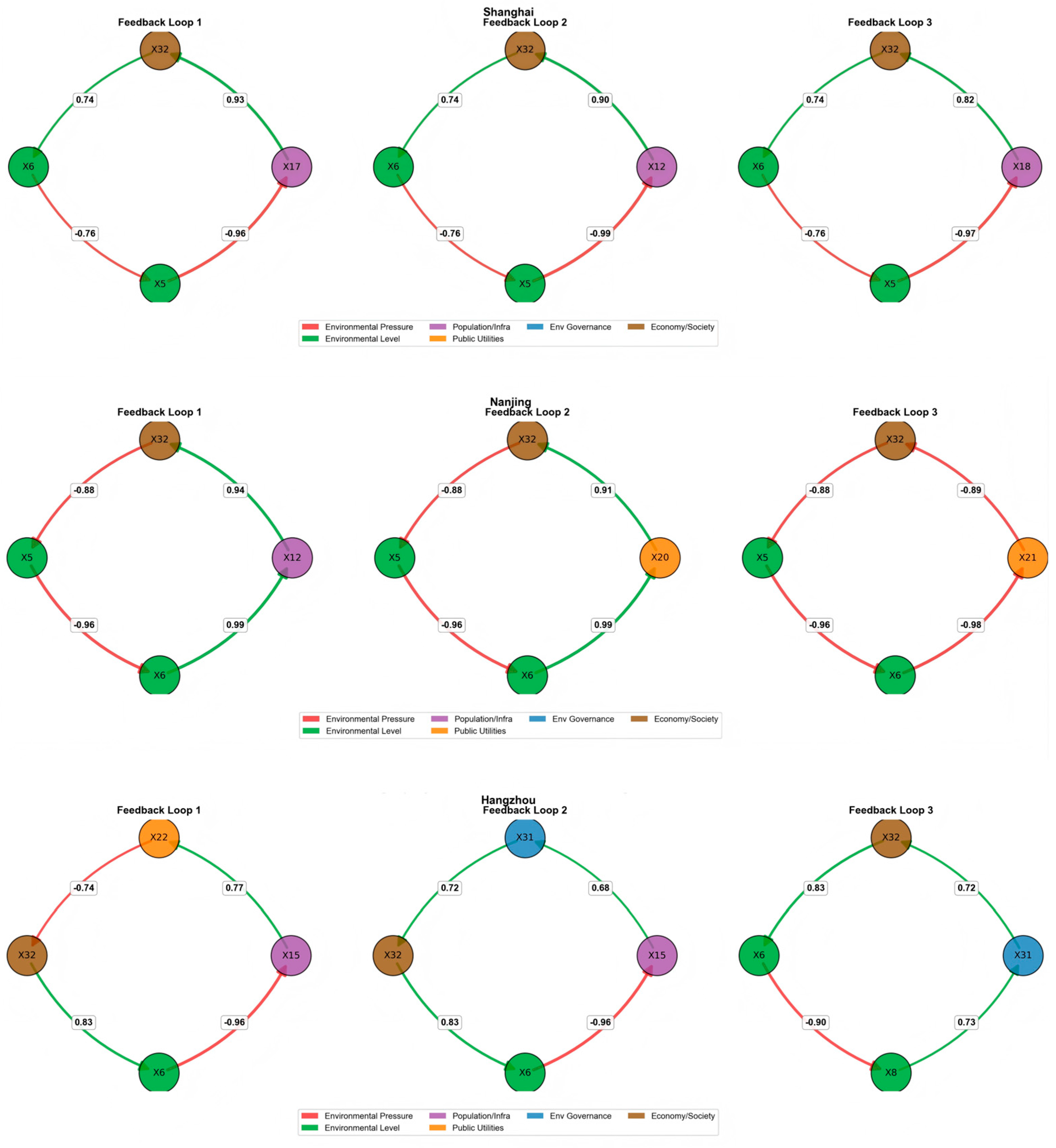
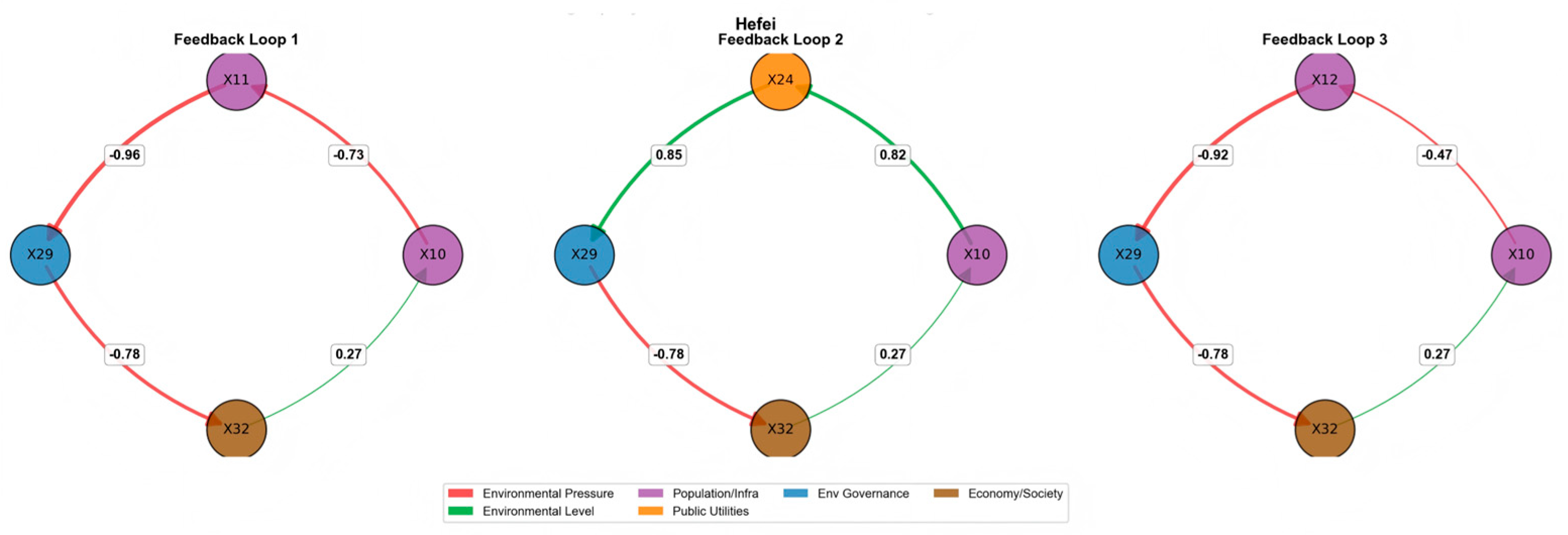
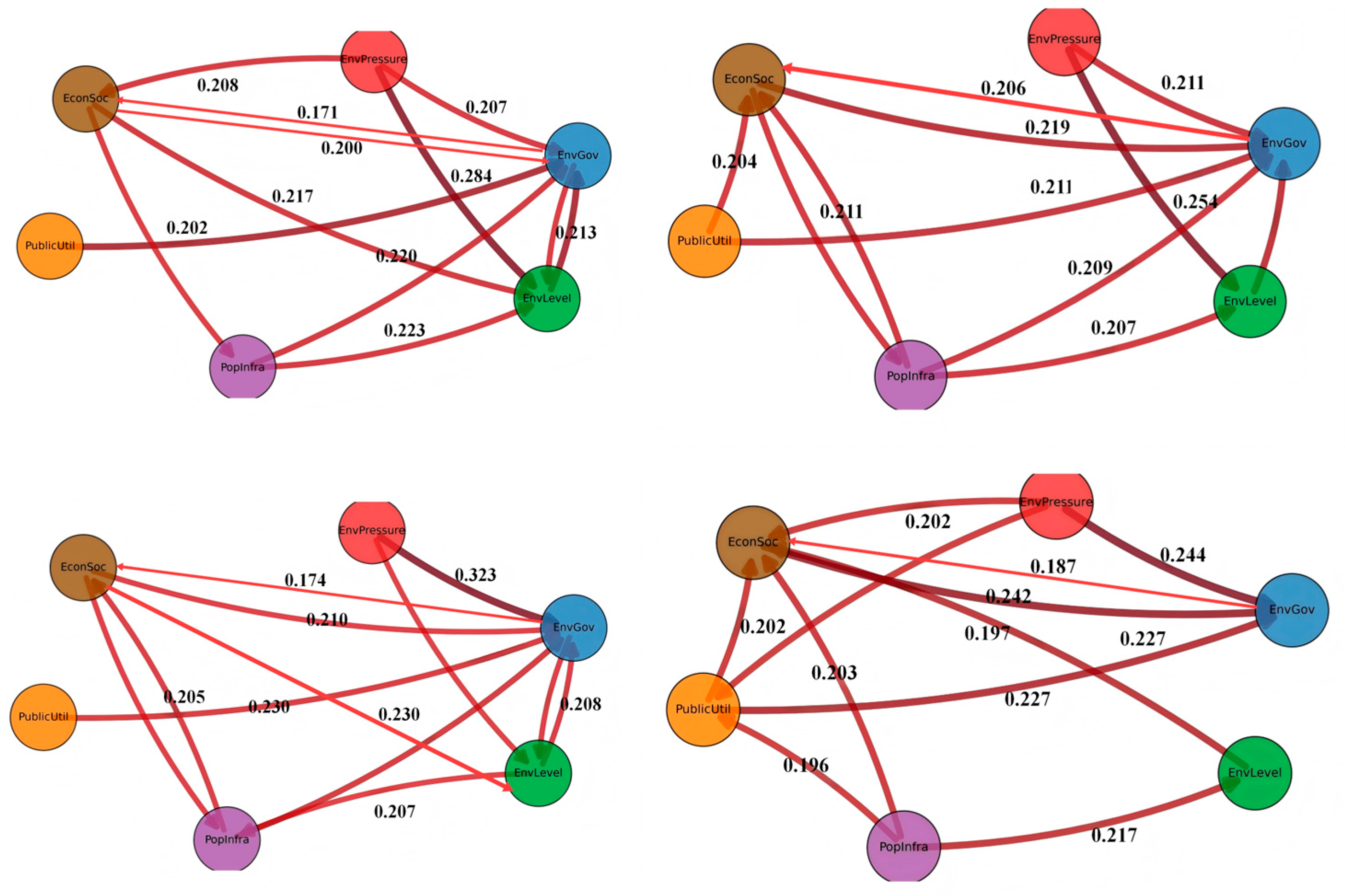
Based on the causal intensity matrix between subsystems of each city, this study further identified the key feedback loops existing among subsystems. A feedback loop reflects the dynamic interaction and mutual restriction among various elements within the system, and its polarity (positive/negative) determines the system’s behavior mode. Through a comparative analysis of four provincial capitals in the Yangtze River Delta region—Shanghai, Nanjing, Hangzhou and Hefei—three types of representative key feedback loops were identified, and the urban heterogeneity of these loops was further analyzed to reveal the differences in system operation mechanisms among cities at different development stages.

4.1.1. Mutual Feedback Loop Between EG and EL

A bidirectional causal relationship exists between the EG and EL subsystems in all analyzed cities, forming a positive feedback loop. In Hangzhou, the causal effect from EG to EL is 0.208, and from EL to EG is 0.211—indicating strong balance. At the indicator level, EG investment (X28) strongly affects environmental quality indicators (X5–X9), with impact intensities of 0.887–0.924; conversely, X5 affects EG investment (X28–X29) at 0.872–0.938. This loop works as follows: increased EG improves air and water quality, which in turn raises public environmental awareness and strengthens government commitment—driving further investment. Its positive polarity creates a self-reinforcing virtuous cycle, accelerating environmental improvement once triggered. Data from Shanghai (loop intensity = 0.213) and Nanjing (0.194) confirm this mechanism operates across cities of different sizes.

4.1.2. Coupled Development Loop Between ES and PI

A strong bidirectional causal relationship exists between the ES and PI, forming the core driver of urban development. In Hefei, the causal intensity is 0.190 from ES to PI and 0.203 inversely, indicating near-equal strength. At the indicator level, X33 (economic output) strongly influences X10–X18 (population and infrastructure indicators) with intensities of 0.640–0.899; conversely, X11–X12 impact X33–X38 at 0.797–0.858. This loop captures urban development’s core dynamic: economic growth spurs population agglomeration and infrastructure upgrades, while better infrastructure and a larger workforce in turn sustain economic and social progress. In Nanjing, both directions of the loop have equal intensity (0.202), indicating perfect balance and strong synergy between socioeconomic development and population-infrastructure advancement. Shanghai shows similar coupling, with intensities of 0.202 and 0.195.

4.1.3. EP Transmission Chain Loop

The EP serves as a control state, indicating that it remains unaltered by other indicators. Instead, it induces changes in other subsystems through clearly defined transmission paths. In Nanjing, the EP directly degrades environmental quality (X5–X9), with impact intensities ranging from 0.856 to 0.930. Subsequently, the degraded environmental quality triggers EG (X28–X29), with intensities ranging from 0.806 to 0.940, thereby forming a three-level chain: from EP to EL to EG (intensities: 0.254 → 0.219 → 0.211). In Hefei, an alternative pathway emerges: from EP to PU to EG (intensity: 0.197), which demonstrates the dual role of PU as both a buffer and an intermediary.

4.1.4. Bidirectional Interaction Loop Between EG and ES

In all four cities, a significant bidirectional causal loop has been established between the EG and ES. This loop represents the most stable feedback structure within the urban environmental system. In terms of causal intensity, Nanjing shows the strongest influence from EG to ES at 0.206, followed by Hefei (0.187), Hangzhou (0.174), and Shanghai (0.171). The reverse influence from ES to EG is also considerable, with Nanjing reaching 0.219, Shanghai 0.200, Hangzhou 0.210, and Hefei 0.242. This bidirectional strong correlation indicates that economic development and environmental governance have formed a mutually reinforcing virtuous cycle. Specifically, economic growth provides financial support for EG, while the improvement of EG promotes economic development by enhancing urban livability and industrial competitiveness. Hefei is the most prominent in this loop, as the impact intensity of the ES on EG (0.242) ranks first among the four cities, which reflects the synergistic effect of high-intensity investment in environmental infrastructure and economic development in the city in recent years.

4.1.5. Triangular Loop of EL-PI-PU

The second key feedback structure is composed of a triangular loop formed by three subsystems: EL, PI, and PU. This loop illustrates the dynamic equilibrium among urban environmental quality, population carrying capacity, and public service supply. Taking Shanghai as an example, the impact intensity of PI on EL amounts to 0.223, and the impact intensity of PU on EL is 0.197. Meanwhile, the impact of EL on PI is 0.181, and that of EL on PU is 0.171. Hangzhou and Nanjing also display similar structural characteristics. It is worth noting that the causal direction of this loop is not completely symmetric. Generally, the influence of population infrastructure and public utilities on the environmental level is stronger than the reverse influence, suggesting that infrastructure construction and public service supply are the main driving forces for improving environmental quality, rather than passive responses to environmental changes. Hangzhou is particularly typical: the intensities of PI on EL (0.207) and EL on PI (0.201) are relatively balanced, which indicates that the city has achieved favorable results in the coordinated development of the environment and population.

4.2. Urban Heterogeneity of Feedback Loops

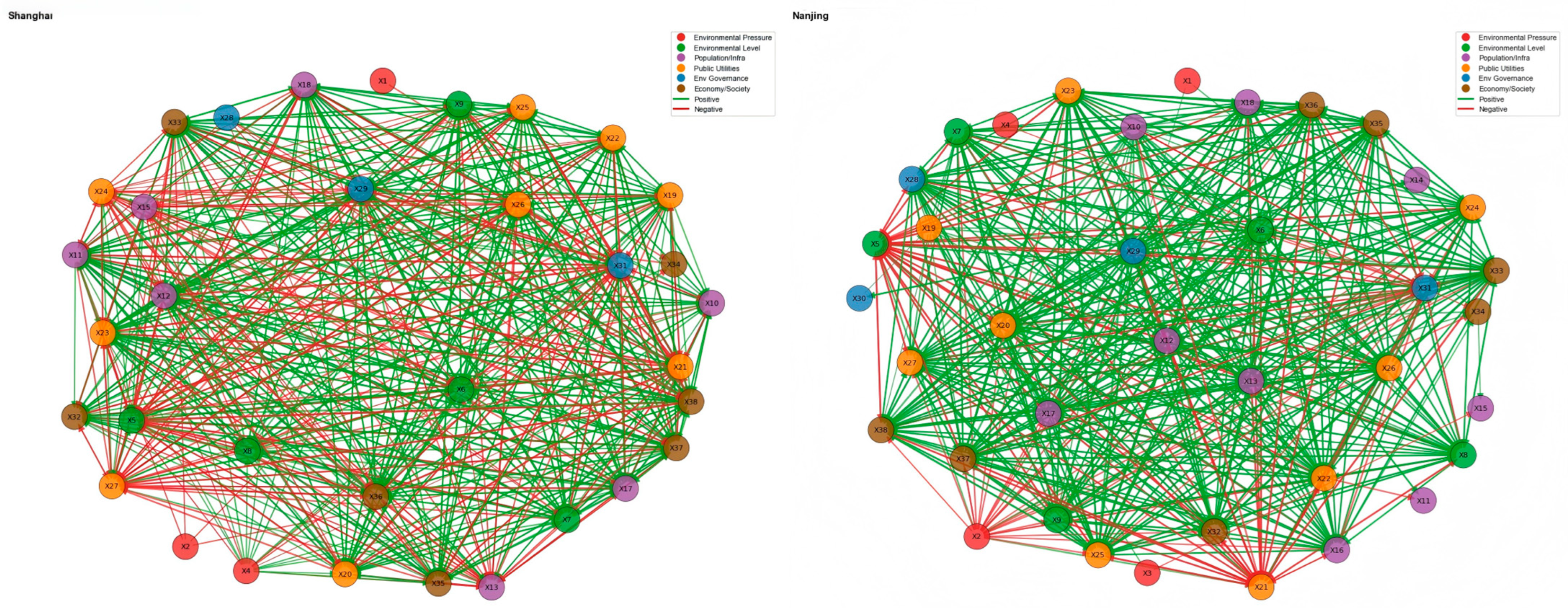
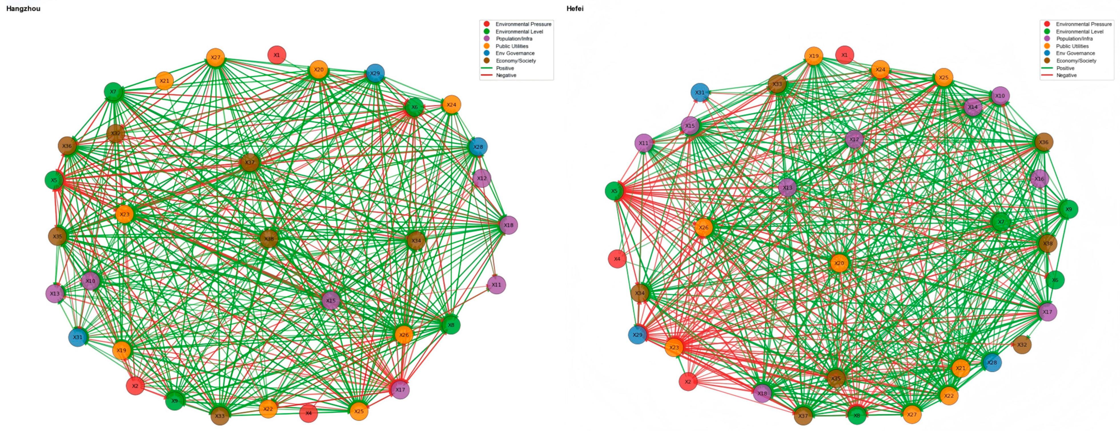
The four cities share common feedback loop structures but also exhibit distinct urban characteristics (Figure 2 and Figure A1). Hangzhou has the densest causal connections among subsystems—averaging 15.3 indicator links per subsystem—forming the most complex network. Shanghai shows a strong unidirectional link: from EP to EL at 0.284, indicating that environmental pressure directly and prominently affects environmental quality. Nanjing features the most complete three-level pressure transmission chain, with all paths exceeding 0.21. Hefei displays strong internal coupling, with PU acting as a core node across multiple loops. All key loops are positive reinforcement loops—reflecting a self-reinforcing cycle where economic/social progress, environmental investment, and improving environmental quality mutually reinforce each other. Yet this also implies “lock-in” risk: a negative shock to any link could amplify system-wide decline. Policy interventions are thus needed to ensure cross-link coordination.

Further analysis of urban heterogeneity shows that different cities have distinct characteristics due to development stages and governance modes. Shanghai has a strong direct path from EP to EL, and the intermediary role of EG is weak (0.207), possibly related to its advanced industrial structure and integrating environmental governance into the management system. In contrast, Hangzhou’s environmental governance subsystem is more central. The intensity from EP to EG reaches 0.323, and bidirectional correlations between EG and other subsystems are well-balanced, reflecting its environmental-governance-centered system regulation. In Nanjing’s loop structure, the bidirectional correlation intensity between the economic and social subsystems and other subsystems is generally high, indicating in-depth integration of economic development and the environmental system. Hefei shows a significantly strong correlation from ES to EG, consistent with the phased characteristics of catch-up construction of environmental infrastructure during its recent rapid urbanization.

In summary, the causal feedback loops between subsystems show the complex interaction mechanisms in the urban environmental system. By systematically analyzing the causal intensity of subsystems in Shanghai, Nanjing, Hangzhou, and Hefei, this study identified three key feedback loop types and their derived structures. These loops have certain common features in different cities, yet also display significant urban heterogeneity, offering targeted insights for urban environmental governance and sustainable development.

4.3. A Causality Similarity Matrix-Based Urban Typology

This study uses causal intensity data from six key urban subsystems (environmental pressure, environmental governance, environmental level, population infrastructure, public utilities, and socioeconomic development) in 41 cities. Each city has 25 causal pathways, with 950 causal intensity records in total. By analyzing these data, the complex interactions among urban subsystems and their regional variations are revealed. Statistically, the environmental level, as the most affected, has the highest average causal intensity (0.2801), showing its significant impact on the ecological environment. Environmental pressure, as the main influencing source, also has an average causal intensity of 0.2801, indicating its dominant driving effect on other subsystems. The mutual influence intensity between subsystems is generally from 0.18 to 0.28, forming a tightly coupled urban operational network.

The average causal strength matrix among subsystems reveals that all the strongest causal pathways point to environmental conditions/level. Specifically, ES → EL strength measures 0.2801, PI → EL is 0.2810, PU → EL is 0.2736, and EG → EL is 0.2749. This indicates that regardless of the starting subsystem, the impact on ecological environment quality remains the most significant. Notably, environmental governance demonstrates strong feedback effects on socioeconomic development with a strength of 0.195, reflecting the regulatory or catalytic role of environmental policies in economic growth. Meanwhile, the interaction between PI and EG is also highly significant, with PI → EG measuring 0.187 and EG →PI 0.197, highlighting the synergistic relationship between population concentration and environmental governance.

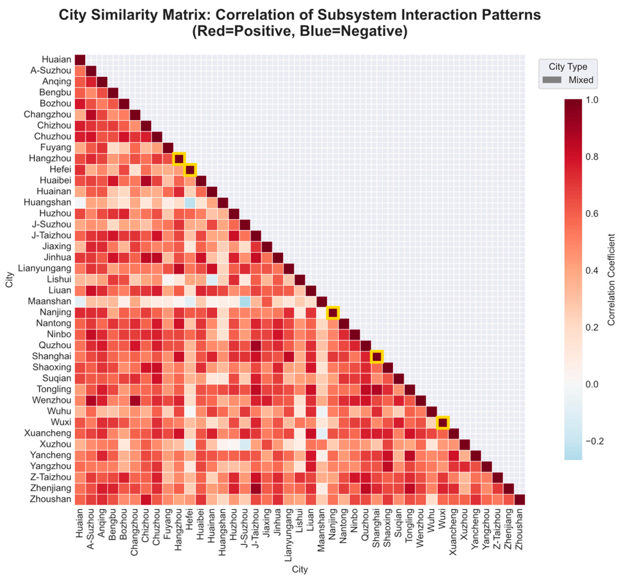
The similarity matrix shows distinct urban clusters, as shown in Figure 3. Through cluster analysis and critical path strength evaluation, 41 cities are classified into four primary types. The economy-driven cluster, led by Tongling with ES → EL strength of 0.4241, includes Lianyungang, Zhoushan, Huaibei, and Suqian. These cities show the most significant direct impact of economic activities on ecological environments, indicating a strong link between economic development and environmental pressures.

The population-infrastructure-driven model is most prominent in Ningbo, with a PI → EL intensity of 0.3534, followed by Yancheng, Zhenjiang, Huai’an, and Nanjing. These cities demonstrate the most significant environmental impacts from population concentration and infrastructure development, highlighting the pronounced environmental effects of urbanization.

The governance-coordinated model is exemplified by Changzhou, showing an EG → EL intensity of 0.2574, with Wuxi, Xuzhou, Wuhu, and Fuyang exhibiting similar characteristics. Their environmental governance measures have proven highly effective in improving ecological conditions, supported by relatively well-established governance systems.

The pressure-response model is most evident in Wuxi (EP → EL intensity: 0.2842), and Xuzhou, Zhenjiang, Yangzhou, and Yancheng also belong to this category. These cities show the direct impact of environmental pressures on ecosystems and clear pressure-response mechanisms.

Regionally, cities in Anhui Province generally have coordinated governance features. Hefei shows a PI-EG coordinated model with a relatively low ES → EL intensity of 0.2438. Wuhu represents an EP-PU-driven model where PU → EL reaches 0.3305. Anqing has balanced development characteristics with intensity evenly distributed across all pathways (0.26–0.30). Fuyang follows the governance-coordinated model, with an EG → EL intensity of 0.2971.

Cities in Jiangsu Province have significant economic–pressure interaction features. Nanjing is population-infrastructure-driven, with a PI → EL intensity of 0.3196. Suzhou represents a mixed economic–pressure model, where EP → EL reaches 0.3239. Wuxi shows a governance-coordination–pressure-response composite model, with EG → EL ratio at 0.2878 and EP → EL ratio at 0.2842, performing remarkably. Xuzhou follows a pressure-governance coordination pattern, with an EP → EL ratio of 0.2745 and an EG → EL ratio of 0.2467, indicating relatively balanced development.

Cities in Zhejiang Province have strong population-driven effects. Hangzhou shows balanced development, with path strength between 0.27 and 0.30. Ningbo, driven by population infrastructure, has the highest provincial PI → EL ratio of 0.3534. Wenzhou belongs to the economic–population coordination model, with ES → EL ratio at 0.2095 and PI → EL ratio at 0.2187, reflecting balanced development. Zhoushan exhibits a mixed economic–pressure model, with an ES → EL ratio of 0.3682 and an EP → EL ratio of 0.2602, showing unique dual-wheel drive characteristics.

This study reaches the following key conclusions: First, the environmental level (EL) is the core response indicator for urban systems. All subsystems have the most significant impact on environmental status, with intensities from 0.273 to 0.281, indicating that ecological environment quality comprehensively reflects urban development. Second, environmental pressure (EP) is the primary driving force, with an average influence of 0.280 on other subsystems, reflecting the reverse pressure mechanism of environmental issues on urban systems. Third, cities can be divided into four types: economy-driven, population-infrastructure-driven, governance-coordinated, and pressure-responsive, each needing different sustainable development strategies. Fourth, regional development patterns have distinct characteristics: Cities in Anhui province generally show governance coordination, cities in Jiangsu have significant economy-pressure interactions, and cities in Zhejiang have prominent population-infrastructure driving effects. Fifth, the most unique city is Suzhou in Jiangsu, with the lowest similarity to other cities (average 0.86–0.90). Tongling’s ES → EL ratio is 0.4241, the highest among all cities, and Hefei has a unique population-public service coordination model.

Based on the findings, the following policy recommendations are proposed. For economy-driven cities like Tongling and Lianyungang, prioritize green industrial transformation to reduce the environmental impacts of economic activities. For population and infrastructure-driven cities such as Ningbo and Yancheng, urban planning should focus on environmental carrying capacity assessments to promote compact urban development. For governance-coordinated cities like Changzhou and Wuxi, summarize and promote successful models of environmental governance-economic development synergy. Moreover, Yangtze River Delta cities should strengthen joint ecological protection and collaborative governance, share environmental governance experiences across regions, and promote coordinated regional development.

4.4. Analysis of Average Impact Intensity Between Subsystems

4.4.1. Impact Intensity Between Subsystems

Regarding the bidirectional interactions among subsystems, pronounced asymmetries are observed in the causal linkages related to environmental governance, as shown in

Table 3. The intensity from the source subsystem to the target subsystem.

Source_Subsystem	Target_Subsystem	Mean	Std	Count
EP	EG	0.258	0.073	37
PI	EG	0.230	0.029	41
ES	EG	0.229	0.027	41
PU	EG	0.229	0.017	41
EL	EG	0.228	0.020	41
EP	EL	0.212	0.060	39
PI	EL	0.202	0.013	41
ES	EL	0.201	0.011	41
PU	EL	0.201	0.011	41
EG	EL	0.199	0.025	41
PU	ES	0.195	0.009	41
ES	PI	0.193	0.014	41
EP	PI	0.192	0.060	41
PU	PI	0.192	0.014	41
PI	ES	0.191	0.013	41
EL	ES	0.190	0.010	41
EG	ES	0.190	0.022	41
EL	PI	0.189	0.015	41
EP	ES	0.189	0.045	41
PI	PU	0.186	0.011	41
ES	PU	0.185	0.013	41
EP	PU	0.184	0.037	41
EL	PU	0.182	0.010	41
EG	PI	0.181	0.025	41
EG	PU	0.178	0.020	41

EP: Environmental_Pressure; EG: Environmental_Governance; PI: Population_Infrastructure; PU: Public_Utilities; ES: Economy_Society; EL: Environmental_Level.

. The positive influence from ES to EG (median ≈ 0.23) is substantially stronger than the reverse effect from EG to ES (median ≈ 0.19). This asymmetry suggests that economic and social dynamics exert a dominant driving force on environmental governance, whereas the feedback effect of governance on the socioeconomic system is relatively weak.

A similar unidirectional pattern appears between PI and EG. The causal strength from PI to EG (median ≈ 0.22) is notably higher than that in the opposite direction (median ≈ 0.18), indicating that population expansion and infrastructure development act as key drivers of environmental governance responses.

In contrast, the bilateral relationship between EG and EL presents a relatively balanced interaction structure. The positive influence of EG on EL (median ≈ 0.21) is marginally stronger than the reverse feedback from EL to EG (median ≈ 0.20). This balanced two-way linkage reflects a reciprocal, adaptive mechanism between governance implementation and environmental conditions.

Among all subsystem pairs, the interaction between ES and PI displays the highest degree of symmetry. The forward causal intensity (ES → PI, median ≈ 0.19) is close to the reverse intensity (PI → ES, median ≈ 0.18), revealing a coordinated co-evolutionary relationship between economic growth and urbanization progress.

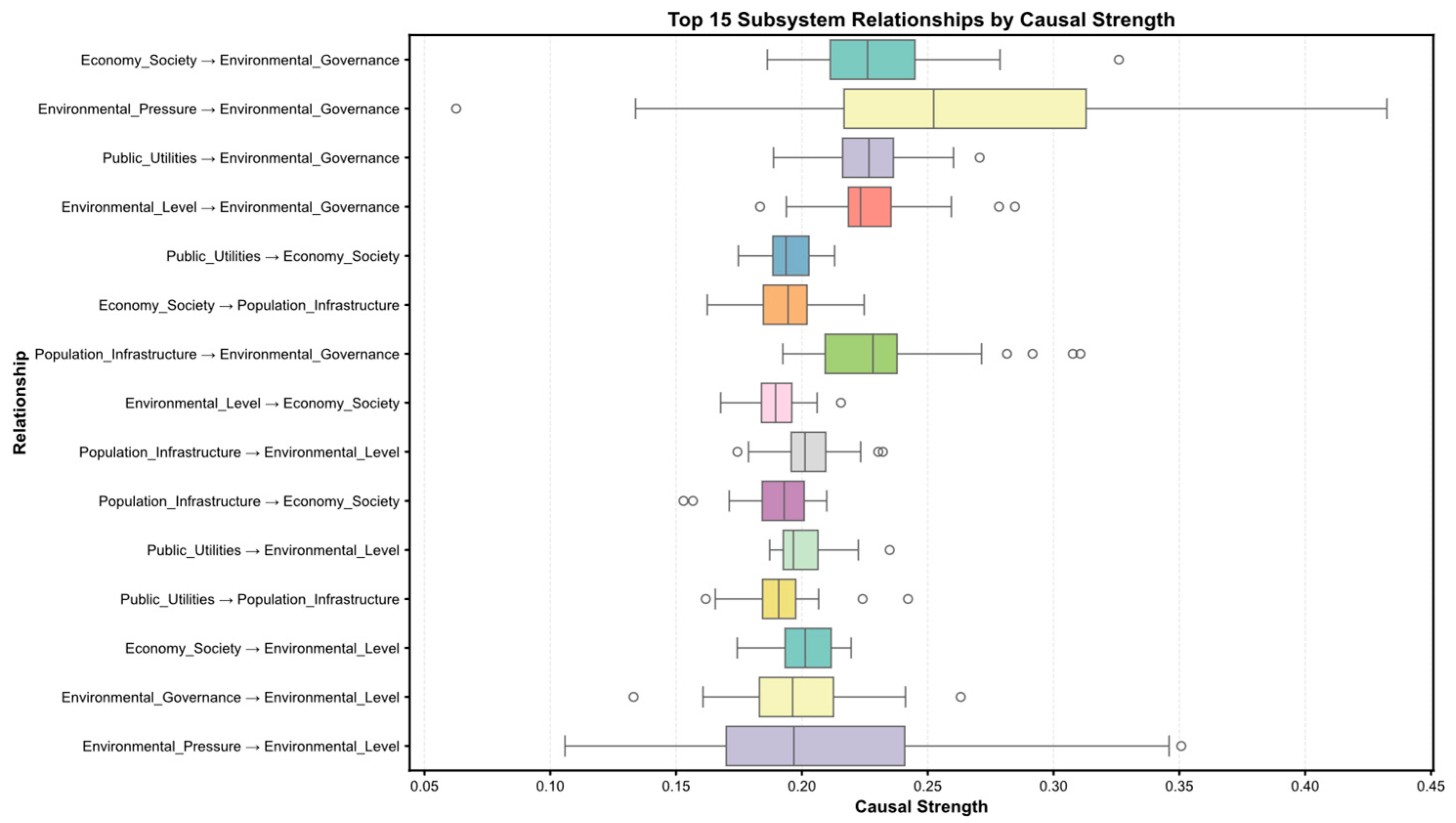
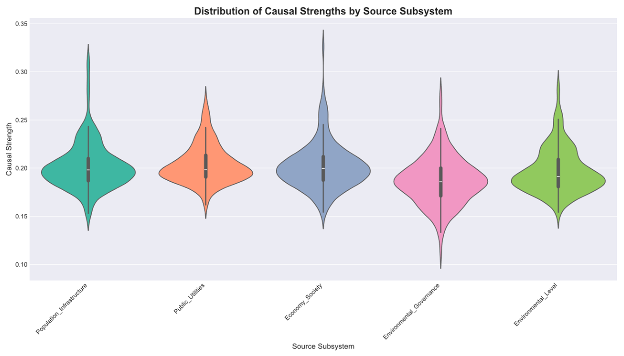
As depicted in the boxplot of the top 15 subsystem relationships ranked by causal strength (Figure 4), linkages directed toward the EG constitute the highest-ranked cluster of causal influences, rather than those directed at the EL itself. This finding refines the conceptualization of the urban system, revealing that environmental governance, rather than the environmental level, acts as the primary integrative node that aggregates pressures from other subsystems.

Specifically, the EP-EG relationship has the highest median causal strength (≈0.25) among top-ranked interactions, along with a relatively wide IQR, suggesting variability in its influence across simulations. Next is the ES-EG linkage, with a median strength of about 0.23 and a narrower IQR, indicating a more consistent influence of economic and social dynamics on environmental governance. The PU-EG and EL-EG relationships rank third and fourth, with median strengths of around 0.21 and 0.20, respectively. Although their IQRs vary, both are prominent in the upper tier of subsystem interactions.

In contrast, linkages directed at the EL, such as those from PI, ES, and EG, exhibit notably lower median causal strengths (≈0.20–0.22) and are positioned lower in the overall ranking. This pattern indicates that the environmental subsystem (EL) is not the ultimate receptor of all subsystem influences, but rather a target of governance interventions that are themselves shaped by broader pressures from the economy, society, and public utilities. Collectively, these results highlight the central role of EG as a critical mediating node that integrates and responds to the cumulative effects of population dynamics, economic activity, public service provision, and environmental pressures within the urban system.

4.4.2. Spatial and Regional Patterns

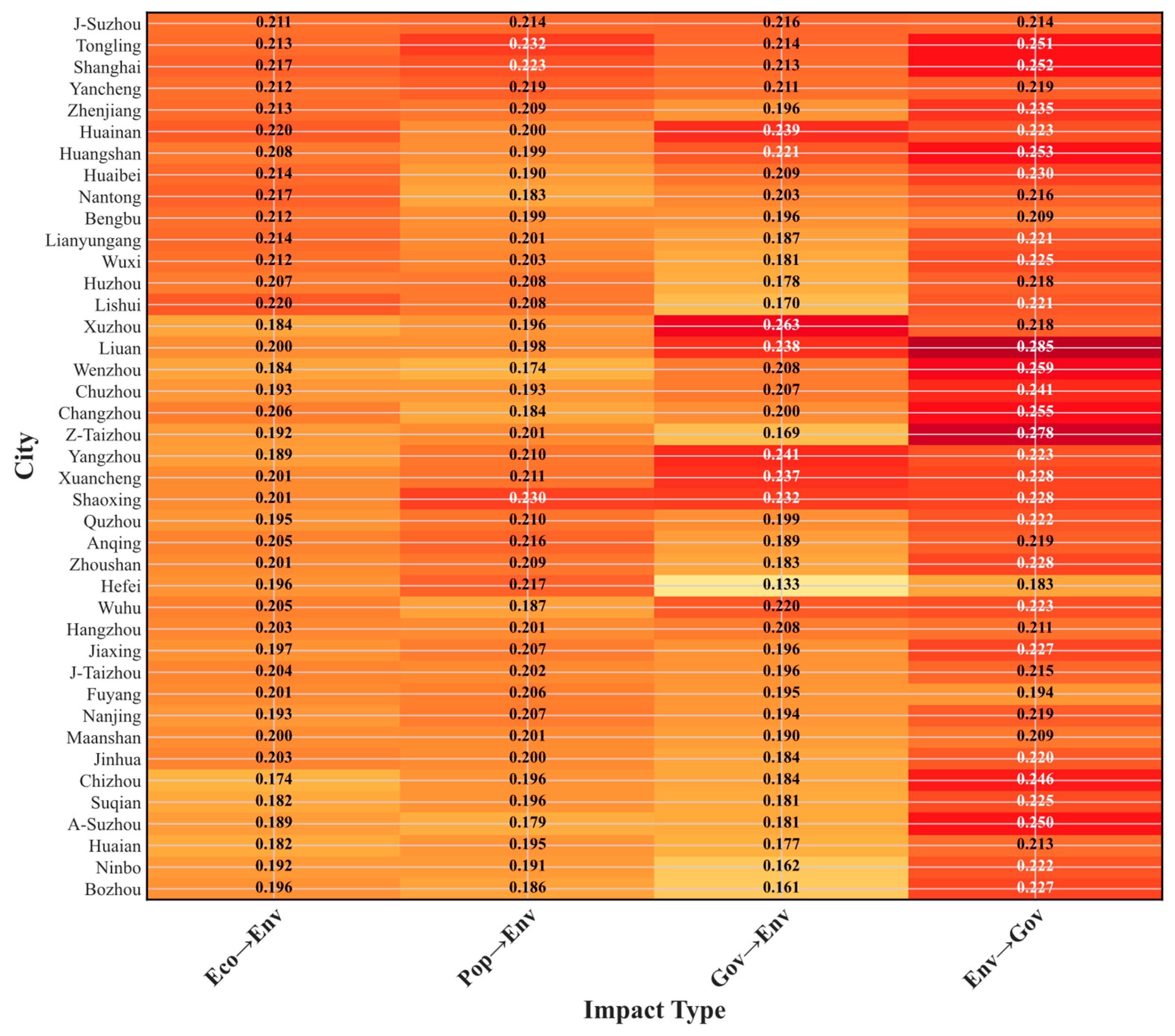
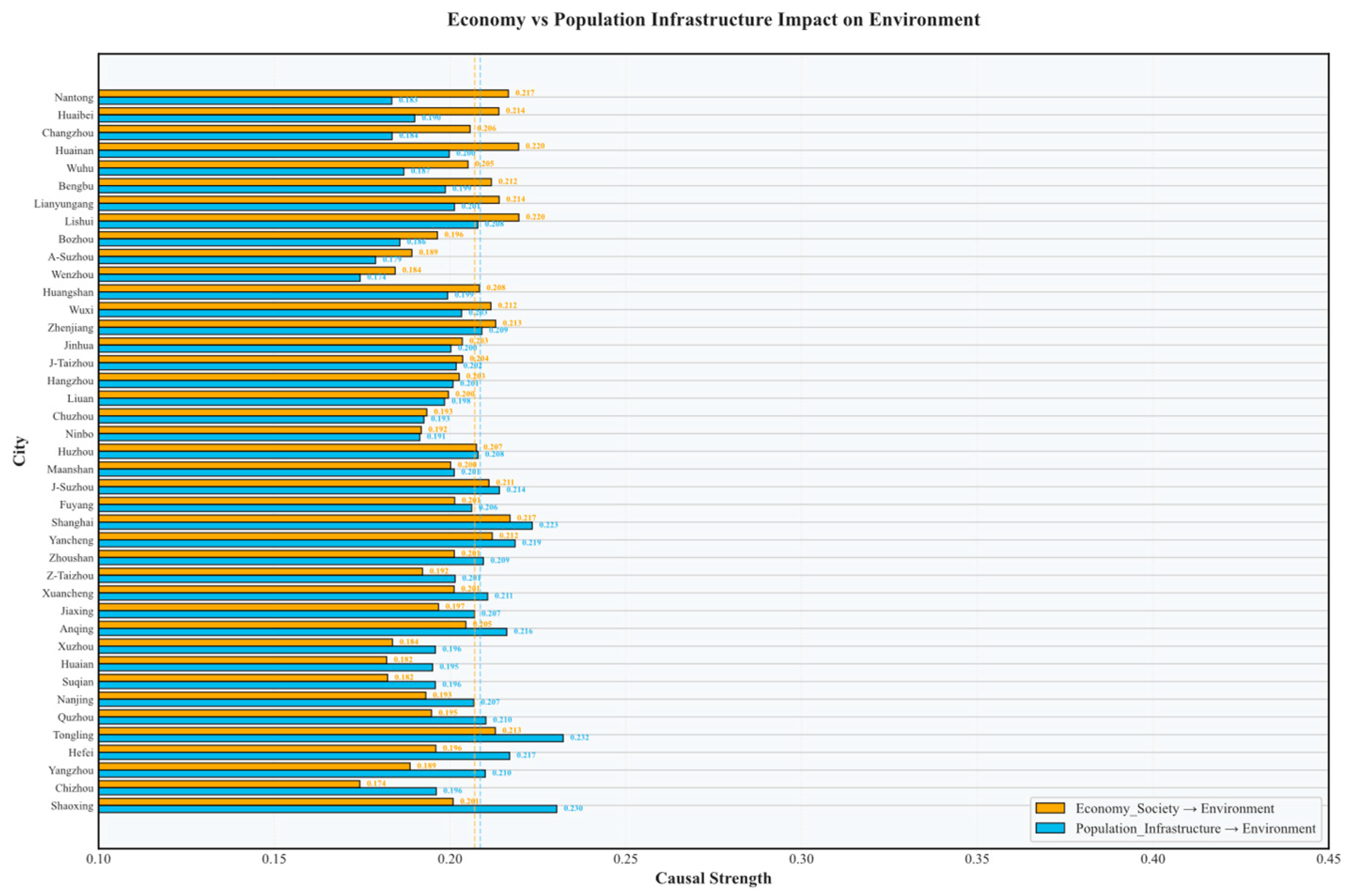
Further analysis of the impact of the economic–social subsystem on the environmental subsystem reveals that this relationship ranks among the most significant in most cities. In cities such as Suzhou (0.211), Tongling (0.213), Shanghai (0.217), Huainan (0.220), and Lishui (0.220), socio-economic activities emerge as the primary drivers of environmental degradation, confirming the strong correlation between economic development and pollution.

Meanwhile, the population and infrastructure subsystems play a more dominant role in certain cities. In cities like Shaoxing (0.230), Tongling (0.232), Shanghai (0.223), and Suzhou (0.214), the population and infrastructure exert a greater environmental influence than socio-economic factors, reflecting these cities’ rapid urbanization phase, where population concentration and urban expansion are the main sources of environmental pressure.

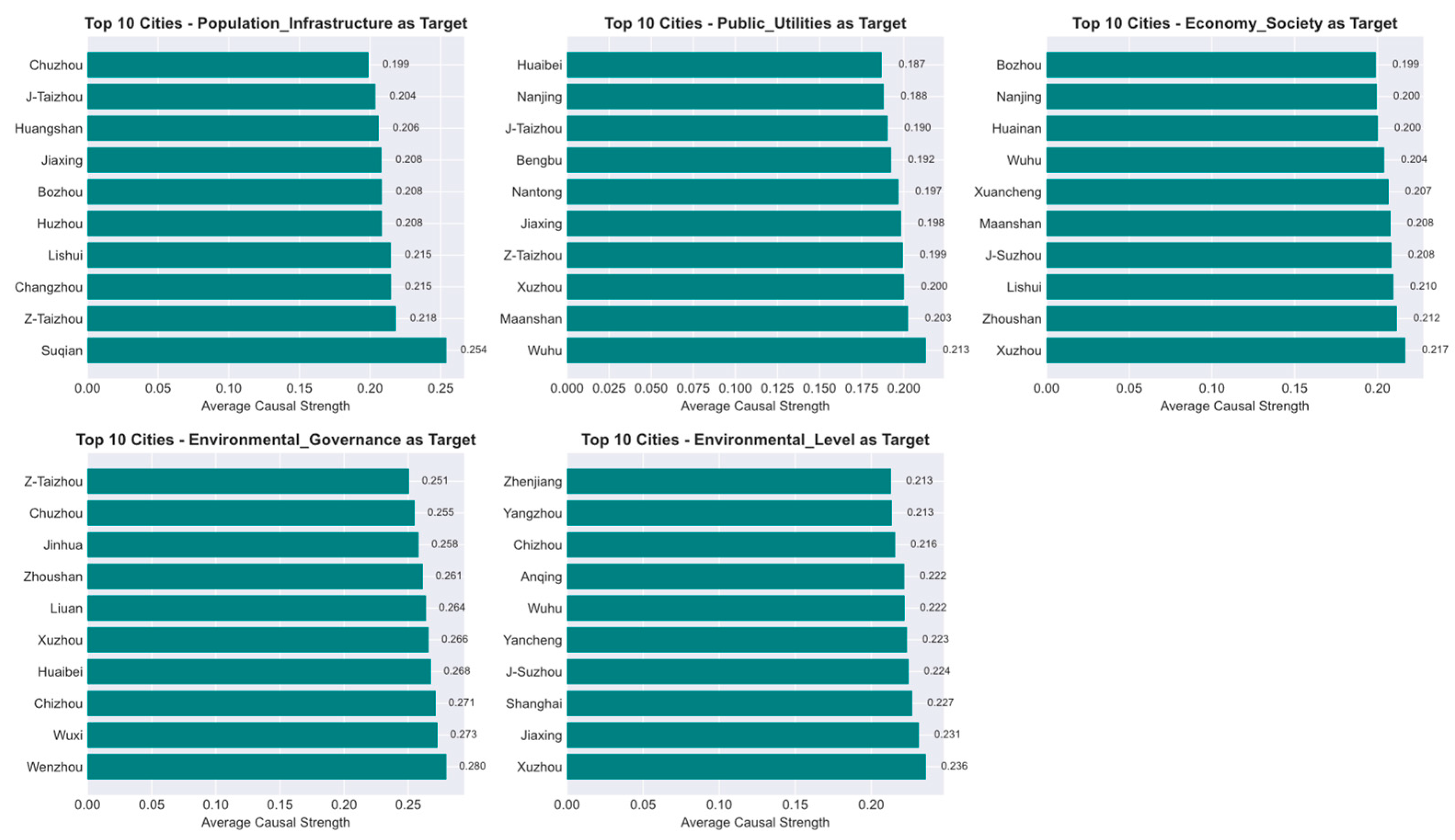
Based on the interaction patterns among subsystems, recall the aforementioned analysis, and sample cities can be preliminarily categorized into four types. Here we display their distribution patterns, as shown in Figure 5.

The first type is economically driven (Eco-Env), represented by Huainan, Huaibei, Wuxi, and Nantong. In these cities, the socioeconomic subsystems exert extremely strong environmental impacts (all exceeding 0.21). These cities are predominantly resource-based and coastal open cities, and economic activities dominate environmental changes.

The second type is population and infrastructure-driven (Pop-Env), exemplified by Shaoxing, Hefei, and Yangzhou. In these cities, the population and infrastructure subsystems demonstrate significant environmental influence. These cities are in rapid urbanization stages, and population concentration and infrastructure expansion are the primary sources of environmental pressure.

The third type is governance-coordinated (Gov ↔ Env), represented by Wenzhou, Changzhou, Taizhou, and Lu’an. In these cities, there are strong bidirectional interactions between environmental governance and environmental conditions. The direct impact of governance on the environment is notable, indicating that these cities have relatively well-established environmental governance systems that can effectively respond to and regulate environmental conditions.

This study employs systematic causal analysis to quantitatively identify and rank bidirectional causal relationships among five subsystems in 41 Chinese cities. A total of 808 statistically significant causal associations (p < 0.05, adjusted for multiple testing) were identified, systematically mapping the directional and intensity distributions of interactions across these subsystems.

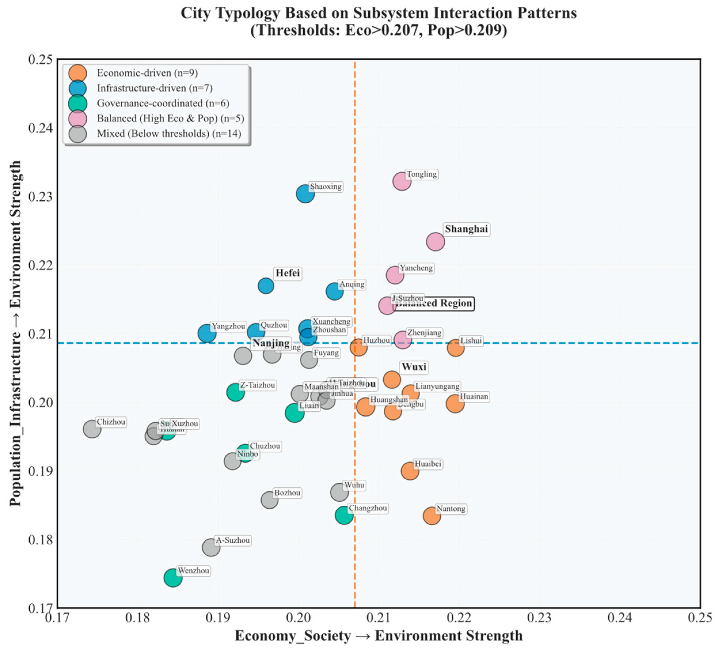
Based on the threshold values derived from the statistical distribution (Eco threshold = 0.207, Pop threshold = 0.209, Gov threshold = 0.223).

Table 4. City typology classification results.

Typology Category	Number of Cities	Percentage	Key Characteristics
Economic-driven	9	22.0%	High Eco → Env (>0.207), Eco > Pop
Infrastructure-driven	7	17.1%	High Pop → Env (>0.209), Pop > Eco
Governance-coordinated	6	14.6%	$\mathrm{High}\mathrm{Gov}\leftrightarrow$ Env (>0.223)
Balanced (High Eco and Pop)	5	12.2%	Both Eco and Pop above thresholds
Mixed (Below thresholds)	14	34.1%	All values below thresholds

classified the 41 cities into five distinct typological categories, and the distribution pattern is shown in Figure 6.

Figure 6 shows the distribution of these cities under different strategy classifications. Economically driven cities (n = 9, n denotes the number of observational cities in the sample) demonstrate a dominant economic influence on environmental outcomes, with Eco-Env strengths (mean = 0.212–0.220) consistently exceeding the impacts of population and infrastructure. Cities such as Huaibei (Eco = 0.214) and Huainan (Eco = 0.220) exemplify this pattern, typically representing industrial and manufacturing centers where economic activities constitute the primary environmental pressure.

Infrastructure-driven cities (n = 7) exhibit the opposite pattern, with Pop-Env (mean = 0.209–0.230) surpassing economic influences. Shaoxing (Pop = 0.230) and Hefei (Pop = 0.217) typify this category, reflecting urban areas where demographic expansion and infrastructure development generate predominant environmental stresses.

Governance-coordinated cities (n = 6) display strong bidirectional Gov ↔ Env interactions (mean = 0.223–0.261), regardless of their economic or population profiles. Lu’an (Gov ↔ Env = 0.261) and Xuzhou (0.241) represent this category, suggesting the presence of effective environmental governance mechanisms that actively respond to and shape environmental conditions.

Balanced cities (n = 5) simultaneously exhibit high economic and population infrastructure impacts (both above thresholds). Shanghai (Eco = 0.217, Pop = 0.223) and Tongling (Eco = 0.213, Pop = 0.232) exemplify this category, typically representing large metropolitan areas where multiple drivers concurrently influence environmental systems.

The majority of cities (34.1%) fall into the mixed category, with all causal strengths below the established thresholds. These cities demonstrate moderate subsystem interactions without any dominant driver, potentially indicating more diffuse or balanced urban-environmental relationships.

The identified typologies carry significant implications for sustainability policy design. Economy-driven cities may require targeted interventions in industrial sectors, while infrastructure-driven cities necessitate a focus on urban planning and demographic management. Governance-coordinated cities offer potential models for institutional mechanisms that effectively mediate human-environment interactions. The substantial proportion of mixed-type cities (34.1%) suggests that many urban areas require integrated policy approaches addressing multiple drivers simultaneously.

5. Discussion

5.1. Governance–Environment Co-Evolution and Demand-Led Regulatory Dynamics

The finding reveals an asymmetric and hierarchical interaction structure among urban subsystems—specifically, Economy Society, Population Infrastructure, and Environmental Governance—within the coupled urban–environmental system. This topology extends the classical pressure–state–response (PSR) framework by incorporating feedback mechanisms and temporal dynamics [23], wherein environmental conditions are typically conceptualized as passive endpoints receiving socioeconomic pressures. This study finds that Environmental Governance functions not as a downstream receptor but as a central integrative node, aggregating and mediating external disturbances originating from socioeconomic and infrastructural domains.

This configuration aligns with recent empirical evidence on governance embeddedness in urban metabolism studies: for instance, Ghosh and Goswami [24] documented similar centrality of institutional capacity in mediating resource flows across Chinese megacities, while Mahtta et al. [25] identified governance institutions as critical “coupling interfaces” between urban expansion trajectories and ecological outcomes in global secondary cities. Crucially, the dominant causal influences from Economy Society and Population Infrastructure onto Environmental Governance suggest that governance responses are primarily reactive and context-dependent—consistent with the “demand-led governance” mechanism described by van den Breil et al. [26] in their analysis of EU urban climate adaptation strategies. In such systems, the scope, timing, and instrumental focus of environmental management are shaped endogenously by the pace and spatial pattern of urban development, rather than by exogenously imposed normative targets or universal technical standards [27,28,29]. This pattern underscores the endogenous co-evolution of governance capacity and urban developmental dynamics—a feature increasingly documented in comparative urban sustainability research [30,31]. It further implies that interventions aimed at strengthening environmental governance must account for path-dependent institutional configurations and the temporal mismatch between infrastructural lifecycles, socioeconomic transitions, and ecological response lags [32].

The observed relatively balanced bidirectional linkage between Environmental Governance and Environmental Level aligns with the conceptual framework of environmental subsystem self-regulation which empirically identified reciprocal feedback loops—where governance interventions shape environmental outcomes, and deteriorating or improving environmental conditions, in turn, trigger adaptive recalibration of institutional arrangements (e.g., policy revision, enforcement intensity, or stakeholder engagement) [33,34]. This finding corroborates the “governance–environment co-evolution” hypothesis advanced in recent urban sustainability literature [35], wherein environmental performance is not merely an output of governance but also a contextual input shaping its design and implementation.

5.2. Interdependence of Economic and Infrastructure Development

The high symmetry in the interaction between Economy Society and Population Infrastructure resonates with established accounts of urban co-development dynamics. Contemporary scholarship has consistently documented the tightly coupled growth trajectories of economic agglomeration and infrastructural expansion in rapidly urbanizing contexts. As Glaeser, Kourtit, and Nijkamp [36] demonstrate cities in the “urban century” exhibit complex evolutionary patterns where agglomeration economies fundamentally shape spatial development. This relationship is further substantiated by Bryan, Glaeser, and Tsivanidis [37], who find that agglomeration benefits in developing-world cities are at least as high as in developed economies, while emphasizing the critical role of infrastructure in moderating the negative externalities of density. Recent empirical studies on large-scale transport infrastructure further validate these dynamics: Nose and Sawada [38] show that highway investments spur manufacturing agglomeration and employment growth in peripheral regions, while Shi et al. [39] demonstrate that high-speed rail networks significantly catalyze industrial upgrading through both economic and administrative externalities. Together, these contemporary analyses confirm that economic and infrastructural systems exhibit interdependent growth trajectories—a relationship that becomes particularly pronounced in rapidly urbanizing contexts. Such coupling reflects structural interdependence rather than unidirectional causality.

This mutual reinforcement constitutes a core mechanism underlying long-term urban system trajectory formation—a mechanism that complexity theorists have long conceptualized as endogenous and path-dependent. Contemporary empirical research has substantiated this theoretical perspective. Lei et al. [40] demonstrate that urban economic development “relies on its previous performance and presents the characteristic of path dependence”. Their findings reveal that urban evolution is shaped by three interdependent forces: local dependence (endogenous agglomeration dynamics), network dependence (interurban interactions), and systemic dependence (relative performance within the urban system). This tripartite framework provides empirical grounding for the systems-theoretic view that cities evolve through the recursive interplay of internal dynamics and external connections, with historical trajectories conditioning future development pathways.

Collectively, these findings emphasize the critical mediating role of environmental governance in the urban system. Effective urban environmental management should not only target improvements in environmental quality but also strengthen the proactive regulatory capacity of governance to reshape its interaction with socioeconomic subsystems. Such a transformation can help alleviate the one-way pressure from urban development on the environment and facilitate a more sustainable and coordinated urban system.

6. Conclusions

This study utilizes panel data from 41 cities in the Yangtze River Delta region spanning 2013–2022 to construct a city environmental system dynamics model comprising 38 indicators. Through causal structure mining and identification of feedback loops between subsystems, the research reveals the internal mechanisms of urban environmental systems and their inherent urban heterogeneity. The key findings are as follows:

Considering causality similarity matrix-based urban typology. This study analyzes causal intensity data from six urban subsystems across 41 cities. It reveals that environmental level subsystem are the most affected (average intensity 0.2801), and environmental pressure subsystem is the strongest driver (also 0.2801). All top causal pathways point to environmental level subsystem, especially those originating from environmental pressure (0.2801), population infrastructure (0.2810), public utilities (0.2736), and environmental governance (0.2749). Environmental governance shows a notable feedback to socioeconomic development (0.195), and there are strong bidirectional links between population infrastructure and environmental governance (0.187 and 0.197). Environmental level are the core response indicator of urban systems. The impacts of subsystems on environmental status range from 0.273 to 0.281, indicating that ecological quality comprehensively reflects urban development. Environmental pressure is the primary driving force, with an average influence of 0.280 on other subsystems, revealing a reverse pressure mechanism.

Cluster analysis groups 41 cities into four types (economy-driven, population-infrastructure-driven, governance-coordinated, and pressure-responsive) based on causal similarity, each needing tailored sustainability strategies. Regional patterns vary: Anhui cities focus on governance coordination; Jiangsu cities have strong economy-pressure interactions; Zhejiang cities highlight population-infrastructure driving effects. Suzhou (Jiangsu) is the most distinctive; Tongling has the highest ES → EL ratio; Hefei has a unique population–public service coordination model. The urban environmental system has three stable core feedback loops. There is a significant bidirectional strong correlation (causal strength 0.17–0.24) between environmental governance and socio-economic subsystems, forming a positive cycle. The triangular loop of environmental quality, population infrastructure, and public utilities reflects a dynamic equilibrium. Environmental pressure, as an exogenous variable, indirectly affects other subsystems through governance actions, creating a chain—like mechanism. The stability of these loops confirms the system’s self-organizing characteristics and provides intervention focal points.

An analysis of Yangtze River Delta provincial capitals shows distinct environmental system operational patterns. Shanghai’s feedback loop has “direct pressure transmission” characteristics, with environmental pressure strongly influencing environmental levels (0.284), and the mediating role of environmental governance being relatively weak due to its integration into routine management during industrial upgrading. Hangzhou is an environmental governance hub. Environmental pressure directly drives governance intensity (0.323), and there are balanced bidirectional connections between governance and other subsystems, presenting a governance-driven optimization model. Nanjing’s socio-economic subsystem has strong interconnections with others, with bidirectional causal relationships above 0.20, showing deep integration of economic development and environmental systems. Hefei has a strong ES → EG correlation (0.242), fitting its catch-up environmental infrastructure construction during rapid urbanization. These differences highlight the need for localized environmental governance strategies by identifying core driving nodes and feedback pathways. Quantitative analysis of subsystem causal relationships offers a scientific basis for policy interventions. The study reveals that population, infrastructure, and public utilities positively impact environmental quality, suggesting infrastructure development and public service provision drive environmental improvement. This guides urban environmental planning to prioritize environmental objectives in infrastructure planning. Additionally, as environmental pressure spreads across subsystems, establishing pressure detection and response mechanisms can turn challenges into governance innovation catalysts.

In conclusion, the urban environmental system constitutes a complex adaptive system composed of multiple elements, with its evolutionary trajectory determined by the structural characteristics of internal feedback loops. The key to enhancing urban environmental governance efficacy lies not in improving individual indicators, but in identifying and optimizing core feedback loops within the system to establish a self-reinforcing virtuous cycle. Future research could validate these findings across larger sample cities while further exploring the temporal evolution patterns of feedback loop strength and their response mechanisms to policy interventions.

7. Limitations and Future Research

The data-driven system dynamics approach developed in this study establishes a novel analytical framework for urban environmental system research. By integrating causal relationship mining, subsystem strength quantification, feedback loop identification, and simulation modeling, this method effectively reconstructs system internal structures under data constraints. It reveals indirect effects and feedback mechanisms that traditional statistical methods often fail to capture, providing a powerful tool for understanding the evolutionary patterns of complex urban environmental systems.

This study acknowledges that the observed coupling patterns among subsystems may be influenced by certain city-level heterogeneities not fully accounted for in the current analytical framework. Specifically, the sample includes cities with variations in administrative status (e.g., municipalities under the State Council, provincial capitals, and prefecture-level cities), primary functional orientations (e.g., resource-based, ecologically focused, or tourism-oriented development profiles), and policy implementation contexts (e.g., designation as pilot zones for environmental governance initiatives). Such differences may contribute to variation in the magnitude or direction of inter-subsystem relationships across cities. For example, the strength of the pressure–response linkage might differ systematically between cities with distinct industrial foundations, and the environmental implications of population agglomeration could vary depending on urban scale and institutional capacity. To further refine understanding of these contextual influences, future work may consider incorporating stratified analytical approaches—such as grouping cities by administrative tier, functional zoning classification (per national spatial planning guidelines), or economic specialization typology. Additionally, integrating formal policy indicators—for instance, inclusion in nationally designated demonstration programs (e.g., National Ecological Civilization Demonstration Areas)—as contextual covariates or interaction terms could help clarify how institutional settings shape coupling dynamics. These refinements would support more nuanced interpretations of pathway mechanisms and inform context-sensitive approaches to urban system governance.

References

1. Wang, X.; Shi, R.; Zhou, Y. Dynamics of urban sprawl and sustainable development in China. Socio-Econ. Plan. Sci. 2020, 70, 100736. [Google Scholar] [CrossRef] [Scilit]
2. Wang, M.; de Vries, W.T.; Sang, W.; Bao, H.; Lyu, Y.; Liu, S. A Method for Delineating Urban Development Boundaries Based on the Urban–Rural Integration Perspective. Land 2025, 14, 859. [Google Scholar] [CrossRef] [Scilit]
3. Shi, Y.; Zhai, G.; Xu, L.; Zhou, S.; Lu, Y.; Liu, H.; Huang, W. Assessment methods of urban system resilience: From the perspective of complex adaptive system theory. Cities 2021, 112, 103141. [Google Scholar] [CrossRef] [Scilit]
4. McPhearson, T.; Haase, D.; Kabisch, N.; Gren, Å. Advancing Understanding of the Complex Nature of Urban Systems; Elsevier: Amsterdam, The Netherlands, 2016; pp. 566–573. [Google Scholar]
5. Xu, G.; Zhu, M.; Chen, B.; Salem, M.; Xu, Z.; Cobbinah, P.B.; Li, X.; Sumari, N.S.; Zhang, X.; Jiao, L. Underlying rules of evolutionary urban systems in Africa. Nat. Cities 2025, 2, 327–335. [Google Scholar] [CrossRef] [Scilit]
6. Jin, X.-B.; Ma, H.; Xie, J.-Y.; Kong, J.; Deveci, M.; Kadry, S. Ada-STGMAT: An adaptive spatio-temporal graph multi-attention network for intelligent time series forecasting in smart cities. Expert Syst. Appl. 2025, 269, 126428. [Google Scholar] [CrossRef] [Scilit]
7. Dong, L.; Shang, J. System dynamics analysis of the coordinated development for urban agglomerations in western China. Environ. Dev. Sustain. 2025, 27, 16053–16090. [Google Scholar]
8. Zhang, L.; Fang, C.; Zhu, C. Coupling coordination and decoupling effects: Measuring the interaction between urban agglomeration ecosystems and urbanization. Cities 2026, 171, 106788. [Google Scholar] [CrossRef] [Scilit]
9. Zhang, F.; Zhang, J.; Hussain, M. The Impact of Multidimensional Regional Integration on Low-Carbon Development: Empirical Evidence from the Yangtze River Delta. Land 2025, 14, 2071. [Google Scholar] [CrossRef] [Scilit]
10. Zolfagharian, M.; Akbari, R.; Fartookzadeh, H. Theory of knowledge in system dynamics models. Found. Sci. 2014, 19, 189–207. [Google Scholar] [CrossRef] [Scilit]
11. Barbrook-Johnson, P.; Penn, A.S. Systems Mapping: How to Build and Use Causal Models of Systems; Springer: Berlin/Heidelberg, Germany, 2022. [Google Scholar]
12. Yin, H.; Zhang, Z.; Wan, Y.; Gao, Z.; Guo, Y.; Xiao, R. Sustainable network analysis and coordinated development simulation of urban agglomerations from multiple perspectives. J. Clean. Prod. 2023, 413, 137378. [Google Scholar] [CrossRef] [Scilit]
13. Li, L.; Ma, S.; Zheng, Y.; Xiao, X. Integrated regional development: Comparison of urban agglomeration policies in China. Land Use Policy 2022, 114, 105939. [Google Scholar] [CrossRef] [Scilit]
14. Zhuang, L.; Ye, C. More sprawl than agglomeration: The multi-scale spatial patterns and industrial characteristics of varied development zones in China. Cities 2023, 140, 104406. [Google Scholar] [CrossRef] [Scilit]
15. Xu, S.; Liu, Q.; Sun, H. Economic coordination development from the perspective of cross-regional urban agglomerations in China. Reg. Sci. Policy Pract. 2022, 14, 36–59. [Google Scholar] [CrossRef] [Scilit]
16. Xu, C.; Xie, D.; Gu, C.; Zhao, P.; Wang, X.; Wang, Y. Sustainable development pathways for energies in Yangtze River Delta urban agglomeration. Sci. Rep. 2023, 13, 18135. [Google Scholar] [CrossRef] [Scilit] [PubMed]
17. Zhang, B.; Shao, D.; Zhang, Z. Spatio-temporal evolution dynamic, effect and governance policy of construction land use in urban agglomeration: Case study of Yangtze River Delta, China. Sustainability 2022, 14, 6204. [Google Scholar] [CrossRef] [Scilit]
18. Guo, Y.; Tong, Z.; Wang, Z.; Xu, Z.; Yao, Y. Evolutionary characteristics and influencing mechanisms of green development efficiency in Chinese urban agglomerations: Analysis of the Yangtze river Delta urban agglomeration. J. Environ. Manag. 2025, 375, 124236. [Google Scholar] [CrossRef] [Scilit]
19. Zheng, L.; Yang, X.; Yu, W.; Zhang, J. Spatiotemporal evolution and configurational pathways of synergistic green development in the Yangtze river economic belt. Sci. Rep. 2026, 16, 7262. [Google Scholar] [CrossRef] [Scilit] [PubMed]
20. Wu, J.; Sun, W. Regional integration and sustainable development in the Yangtze River Delta, China: Towards a conceptual framework and research agenda. Land 2023, 12, 470. [Google Scholar] [CrossRef] [Scilit]
21. Alberti, M. Advances in Urban Ecology: Integrating Humans and Ecological Processes in Urban Ecosystems; Springer: Berlin/Heidelberg, Germany, 2008. [Google Scholar]
22. World Health Organization. World Health Statistics 2016 [OP]: Monitoring Health for the Sustainable Development Goals (SDGs); World Health Organization: Geneva, Switzerland, 2016. [Google Scholar]
23. Niemeijer, D.; De Groot, R.S. A conceptual framework for selecting environmental indicator sets. Ecol. Indic. 2008, 8, 14–25. [Google Scholar] [CrossRef] [Scilit]
24. Ghosh, N.; Goswami, A. Sustainability Science for Social, Economic, and Environmental Development; IGI Global: Palmdale, PA, USA, 2014. [Google Scholar]
25. Mahtta, R.; Fragkias, M.; Güneralp, B.; Mahendra, A.; Reba, M.; Wentz, E.A.; Seto, K.C. Urban land expansion: The role of population and economic growth for 300+ cities. NPJ Urban Sustain. 2022, 2, 5. [Google Scholar] [CrossRef] [Scilit]
26. Breil, M.; Zandersen, M.; Pishmisheva, P.; Pedersen, A.B.; Romanovska, L.; Coninx, I.; Rogger, M.; Johnson, K. ‘Leaving No One Behind’ in Climate Resilience Policy and Practice in Europe: Overview of Knowledge and Practice for Just Resilience. 2021. ETC/CCA Technical Paper Vol. 2021 No. 2. Available online: https://www.eionet.europa.eu/etcs/etc-cca/products/etc-cca-reports/tp_2-2021 (accessed on 14 March 2026).
27. Anguelovski, I.; Shi, L.; Chu, E.; Gallagher, D.; Goh, K.; Lamb, Z.; Reeve, K.; Teicher, H. Equity impacts of urban land use planning for climate adaptation: Critical perspectives from the global north and south. J. Plan. Educ. Res. 2016, 36, 333–348. [Google Scholar] [CrossRef] [Scilit]
28. Bulkeley, H.; Castán Broto, V.; Maassen, A. Low-carbon transitions and the reconfiguration of urban infrastructure. Urban Stud. 2014, 51, 1471–1486. [Google Scholar] [CrossRef] [Scilit]
29. Abel, D. The role of networked governance for local climate policy output. Evidence from Europe. Environ. Politics 2026, 35, 315–337. [Google Scholar] [CrossRef] [Scilit]
30. Wolch, J.R.; Byrne, J.; Newell, J.P. Urban green space, public health, and environmental justice: The challenge of making cities ‘just green enough’. Landsc. Urban Plan. 2014, 125, 234–244. [Google Scholar] [CrossRef] [Scilit]
31. Hu, X.; Yang, C. Institutional change and divergent economic resilience: Path development of two resource-depleted cities in China. Urban Stud. 2019, 56, 3466–3485. [Google Scholar] [CrossRef] [Scilit]
32. Hocherman, T.; Trop, T.; Ghermandi, A. Time lags in environmental governance: A critical review. Ambio 2025, 54, 2042–2059. [Google Scholar] [CrossRef] [Scilit] [PubMed]
33. Panayotou, T. Demystifying the environmental Kuznets curve: Turning a black box into a policy tool. Environ. Dev. Econ. 1997, 2, 465–484. [Google Scholar] [CrossRef] [Scilit]
34. Ridwan, M.; Akther, A.; Dhar, B.K.; Roshid, M.M.; Mahjabin, T.; Bala, S.; Hossain, H. Advancing circular economy for climate change mitigation and sustainable development in the nordic region. Sustain. Dev. 2025, 33, 225–244. [Google Scholar] [CrossRef] [Scilit]
35. Yu, B.; Zhang, Z.; Jiang, M.; Wang, J.; Lee, K.E.; Abdul Halim, S.; Zheng, X. An evolutionary governance framework for the sustainable management of urban wetlands: Integrating theoretical perspectives and practical applications. Sustain. Sci. 2026, 21, 809–837. [Google Scholar] [CrossRef] [Scilit]
36. Glaeser, E.; Kourtit, K.; Nijkamp, P. Urban Empires; Routledge London: London, UK, 2020. [Google Scholar]
37. Bryan, G.; Glaeser, E.; Tsivanidis, N. Cities in the developing world. Annu. Rev. Econ. 2020, 12, 273–297. [Google Scholar] [CrossRef] [Scilit]
38. Nose, M.; Sawada, Y. From Battlefield to Marketplace: Industrialization via Interregional Highway Investments in the Greater Mekong Sub-Region; Institute for Economics Studies, Keio University: Minato, Japan, 2025. [Google Scholar]
39. Shi, D.; Wang, L.; Zhang, X.; Yu, T. Borrowed size and borrowed administrative power: Effects of high-speed rail network on industrial upgrading and variegated externalities in the Yangtze River Delta, China. J. Transp. Geogr. 2025, 123, 104113. [Google Scholar] [CrossRef] [Scilit]
40. Lei, W.; Jiao, L.; Xu, Z.; Xu, G.; Zhou, Z.; Luo, X. Effects of local, network and systemic dependence on urban development. Sustain. Cities Soc. 2022, 86, 104134. [Google Scholar] [CrossRef] [Scilit]
Figure 1. Schematic illustration of the study area.
Land 15 00482 g001
Figure 2. Key feedback loops with causal strengths among Shanghai, Nanjing, Hangzhou and Hefei.
Land 15 00482 g002aLand 15 00482 g002b
Figure 3. Correlation matrix: city similarity based on subsystem interactions. Note: The color mapping range was set from −4 to 0, corresponding to the original strength of 0.0001 to 1. Specific values were labeled in the heatmap to facilitate accurate comparison. The yellow squares mark the five cities of Shanghai, Nanjing, Hangzhou, Hefei and Wuxi.
Land 15 00482 g003
Figure 4. Top 15 subsystem relationships by causal strength. Note: Each row represents a directional relationship (Source → Target), with relationships ordered from highest to lowest median causal strength (top to bottom). The box indicates the interquartile range (IQR: 25–75th percentile), the vertical line within the box marks the median, whiskers extend to 1.5× IQR, and points beyond represent outlier cities with exceptional values. Colors follow the Set3 categorical colormap to enhance visual distinction between relationships. Wider distributions indicate greater cross-city variability in that causal pathway, while consistent patterns suggest more universal subsystem interactions. The x-axis shows causal strength values, enabling direct comparison of effect magnitudes across different subsystem pairs.
Land 15 00482 g004
Figure 5. Causal strength system impact patterns across cities. Note: The heatmap shows causal strengths for four relationships (Eco → Env, Pop → Env, Gov → Env, Env → Gov) using a yellow-orange-red gradient: lighter yellow (≈0.10) indicates weaker relationships, transitioning through orange (≈0.15–0.22) to dark red (≈0.30) indicating stronger relationships. The continuous color scale enables rapid identification of dominant interaction patterns.
Land 15 00482 g005
Figure 6. City typology based on subsystem interaction patterns. Note: Cities are sorted by classification type (Balanced, Economic-driven, Infrastructure-driven, Governance-coordinated, Mixed) with colored dots indicating type. Thresholds for each relationship were calculated as mean + 0.5 × standard deviation of the causal strengths across all cities. This data-driven approach ensures thresholds reflect the natural distribution of causal strengths while providing meaningful separation between city types.
Land 15 00482 g006