1. Introduction
Wetlands are critical ecosystems that provide essential services such as water purification, flood regulation, and habitats for diverse species [
1,
2,
3,
4,
5,
6]. However, these ecosystems are increasingly threatened by global degradation driven by climate change and intensifying human activities, including urban expansion, agricultural development, and pollution. China’s coastal wetlands are particularly vulnerable, having experienced substantial loss and alteration over recent decades. It is estimated that approximately 50% of China’s natural coastal wetlands were lost between 1950 and 2000 [
7,
8,
9,
10], underscoring the urgent need for long-term monitoring. Continuous observation is essential for detecting changes and providing scientific support for effective conservation and management.
Remote sensing has proven highly effective for wetland mapping, with numerous datasets developed to represent specific wetland types, such as floods, mangroves, and mudflats [
11,
12,
13,
14,
15,
16,
17,
18]. While these datasets provide valuable thematic information, many focus on individual wetland categories and do not comprehensively represent the full diversity of wetland ecosystems. In contrast, land use/land cover change (LUCC) products offer broader spatial coverage but often lack the thematic detail required for fine-scale wetland classification [
19,
20,
21]. Previous studies have reported relatively low classification accuracy for wetlands in global LUCC products, reflecting persistent challenges in discriminating spectrally similar wetland classes [
22,
23].
Several global and national wetland datasets have sought to improve thematic detail and mapping accuracy. The Global Lakes and Wetlands Database (GLWD) provides a widely used global wetland inventory but is constrained by coarse spatial resolution and legacy data sources [
24,
25,
26]. National datasets such as CAS_Wetlands [
27] and the China Land Use/Cover Dataset (CLUD) [
28] offer more detailed wetland classifications. Nevertheless, these datasets are typically produced for specific time periods and often depend on extensive visual interpretation, which increases production costs and introduces uncertainties related to subjectivity, temporal inconsistency, and transferability. These limitations indicate that existing datasets, while valuable, may not fully support long-term, fine-scale wetland monitoring across diverse coastal environments.
Optical satellite imagery—including Landsat, Sentinel-2, and MODIS—offers rich spectral information that is highly valuable for wetland mapping [
29,
30,
31,
32]. Landsat, with its long temporal coverage and moderate spatial resolution, is particularly suited for wetland monitoring [
27]. However, cloud contamination and seasonal variability pose persistent challenges in coastal regions. Recent studies have demonstrated that integrating Landsat time-series data with cloud computing platforms such as Google Earth Engine (GEE) can effectively reduce data gaps and enhance classification performance [
33,
34,
35,
36]. Large-scale, time-series-based wetland products derived from Landsat imagery have also been developed at regional and global scales, highlighting the potential of temporal information for characterizing wetland dynamics [
37].
In parallel, a wide range of classification approaches has been explored for wetland mapping. Traditional supervised classifiers, including Maximum Likelihood Classification (MLC), Support Vector Machines (SVM), and Random Forest (RF), remain widely used due to their robustness and computational efficiency [
38,
39,
40]. More recently, deep learning-based approaches, such as convolutional neural networks and Transformer architectures, have shown promising results in land-cover and wetland mapping by leveraging spatial context and hierarchical feature representation [
41,
42,
43]. These methods have demonstrated improved performance in complex environments but often require large, high-quality training datasets and substantial computational resources, which may limit their applicability in large-scale or long-term monitoring tasks [
44].
Despite these advances, accurately distinguishing diverse wetland subtypes—such as rivers, lakes, ponds, paddy fields, tidal flats, and mangroves—remains challenging due to spectral similarity, temporal variability, and complex spatial patterns in coastal environments. Pixel-based classifiers frequently struggle with class confusion, while object-based approaches relying on manually defined rules may suffer from subjectivity and limited transferability across regions [
45,
46,
47,
48]. These challenges underscore a broader need for classification frameworks that balance automation, interpretability, and scalability while explicitly accounting for uncertainty.
Against this background, this study develops a two-step classification framework that integrates pixel-level Random Forest classification with object-based hierarchical decision-tree refinement to map detailed wetland types in China’s coastal regions using Landsat-8 time-series imagery. The objectives of this study are to: (1) construct a detailed classification system encompassing 10 wetland and 5 non-wetland types; (2) evaluate the classification accuracy and uncertainty of the proposed framework; and (3) assess the effectiveness of the two-step strategy in reducing misclassification among spectrally similar wetland features. The results aim to provide a consistent and transparent basis for coastal wetland analysis and long-term ecological monitoring within the Chinese coastal context.
2. Materials and Methods
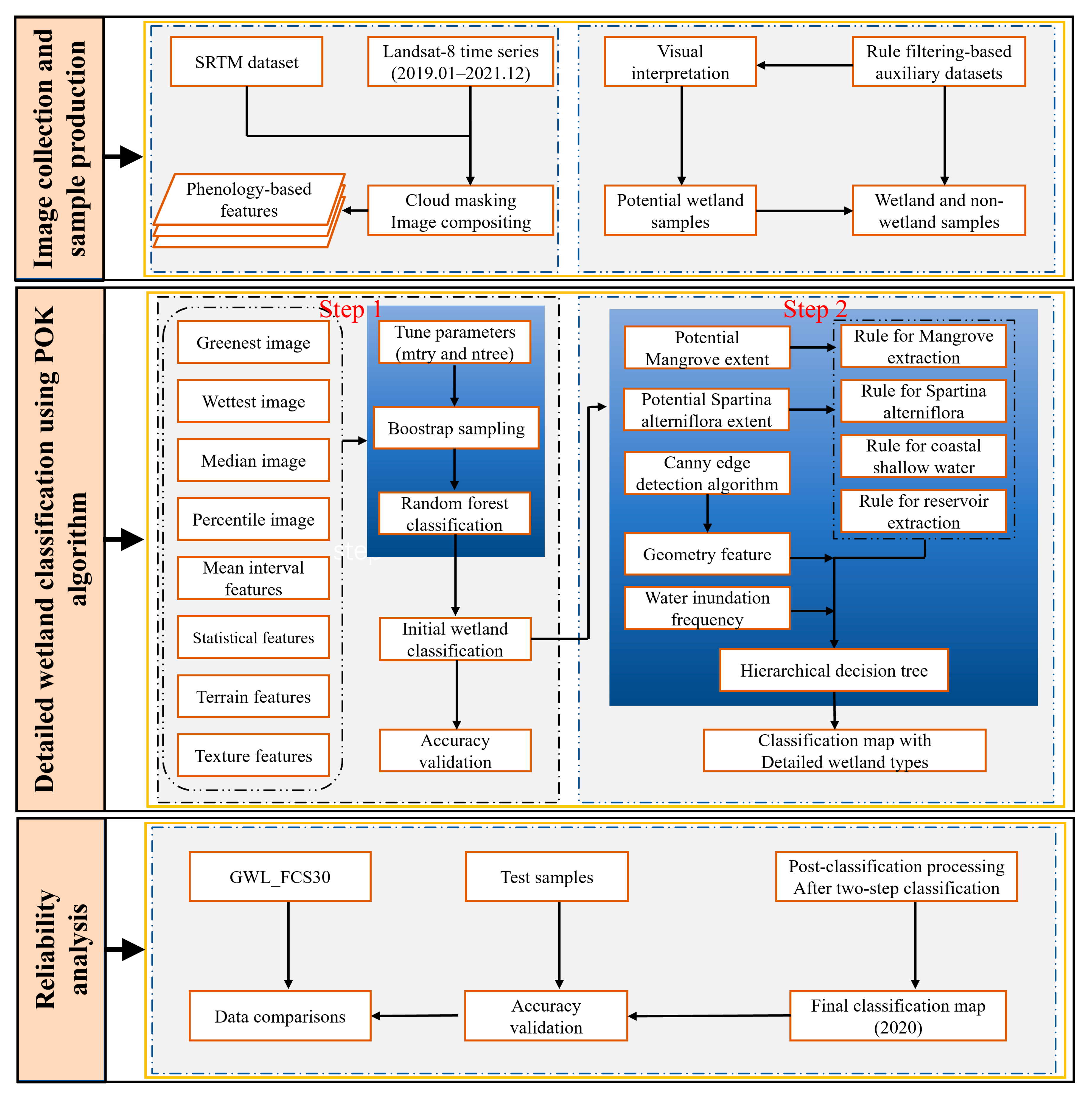
This study proposes a novel approach for fine-scale wetland type classification in China’s coastal regions. The overall workflow consists of three major stages: (1) selecting satellite imagery and generating training samples; (2) applying a two-step classification framework that integrates pixel-based and object-based methods; and (3) evaluating classification accuracy using independent validation samples and Landsat-8 imagery. As il-lustrated in
Figure 1, the workflow includes two color-coded modules. The first blue box represents the pixel-based classification stage, where a Random Forest algorithm produces the initial classification. The second blue box represents the object-based refinement stage, and its dashed box highlights a set of rule-based submodules designed to extract specific wetland types such as mangroves, salt marshes, shallow coastal waters, and reservoirs.
2.1. Study Area
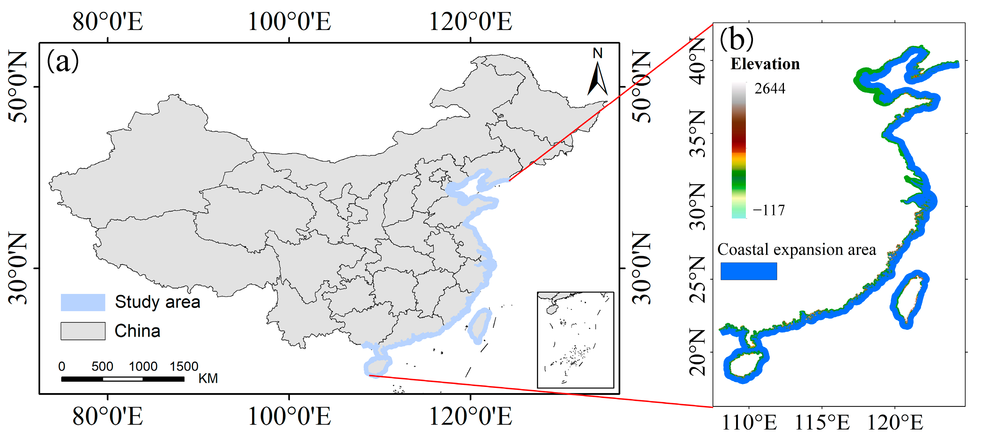
This study focuses on coastal wetlands distributed along China’s eastern seaboard. The study area encompasses 12 provincial-level administrative regions: Liaoning, Hebei, Tianjin, Shandong, Jiangsu, Shanghai, Zhejiang, Fujian, Guangdong, Guangxi, Hainan, and Taiwan. These coastal provinces represent the entirety of China’s shoreline, where wetland ecosystems are shaped by the combined influence of terrestrial and marine processes.
According to the Ramsar Convention, wetlands are defined as areas with water depths less than 6 m. However, due to tidal fluctuations and uncertainties in bathy-metric data, important wetland types—such as mangroves and tidal flats—may be peri-odically exposed at low tide. To ensure complete coverage of potential wetland areas, some studies extend the depth threshold to 25 m [
40,
49]. Accordingly, we adopted a spatial buffer extending 10 km inland and 40 km offshore from the coastline. This boundary encompasses inland and coastal wetlands, including estuarine and nearshore environments where water depths generally do not exceed 25 m (
Figure 2).
2.2. Wetland Classification System
We developed a wetland ecosystem classification system based on the distinguishability of wetland types in medium-resolution satellite imagery, drawing on previous Landsat-based and remote sensing-based wetland classification studies [
27,
50]. The selected wetland classes represent major ecological functions and dominant wetland types in China’s coastal regions. These include two inland wetlands (rivers and lakes), five coastal wetlands (mangroves, salt marshes, tidal flats, coastal aquaculture ponds, and shallow coastal waters), and three artificial wetlands (reservoirs, paddy fields, and agricultural ponds). All classes are distinguishable in Landsat imagery and contribute significantly to coastal ecosystem services.
To produce a complete classification map and enhance the separability of wetland and non-wetland features, five non-wetland land cover types—forest, grassland, built-up land, dryland, and bare land—were also included.
2.3. Data Sources
2.3.1. Landsat Imagery
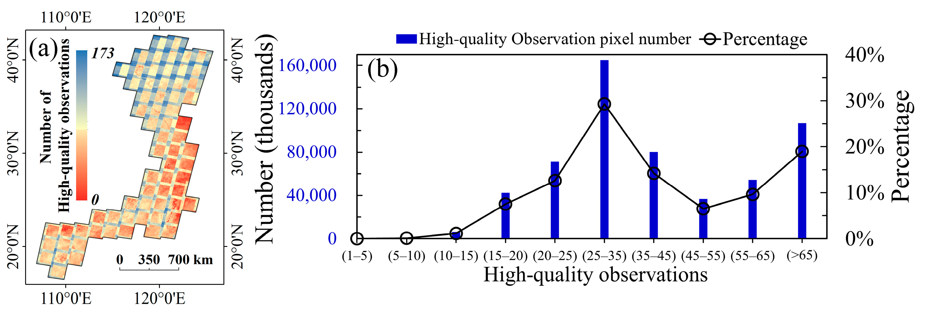
We used Landsat-8 surface reflectance data from the Google Earth Engine (GEE) platform to perform wetland classification for the year 2020. Images from June 2019 to June 2021 were selected, totaling 3641 scenes. To mitigate the effects of cloud contamination, the “QA_PIXEL” band was used to mask low-quality observations.
Figure 3a displays the spatial distribution of cloud-free pixels, and
Figure 3b shows the number of valid observations per pixel. The study area was fully covered by high-quality data, with over 99.9% of pixels having more than five cloud-free observations and over 98.9% having more than 10.
2.3.2. Auxiliary Datasets
We compiled eight categories of auxiliary datasets, including water bodies, tidal flats, mangroves, salt marshes, coastal aquaculture ponds, land use/cover change (LUCC), topography, and other supporting datasets.
Table 1 summarizes the datasets used for sampling, classification, and comparative analysis.
The LUCC category includes the China Land Cover Dataset (CLCD), which provides accurate information for major land types, especially forests, water bodies, and built-up areas. Reservoir extraction utilized Points of Interest (POI), GOODD, and OSM_Dam datasets. Mangrove and Spartina alterniflora datasets were integrated into the Potential Mangrove Extent and Potential Salt Marsh Extent layers to improve identification.
2.4. Training Sample Generation
To generate training samples (i.e., representative land-cover points with known category labels), this study employed a two-stage strategy combining automatic extraction based on auxiliary datasets and visual interpretation with manual screening. The training samples were represented as point data, with each point corresponding to a homogeneous area of a specific land-cover class and distributed across 12 coastal provincial administrative regions in China, including Liaoning, Hebei, Tianjin, Shandong, Jiangsu, Shanghai, Zhejiang, Fujian, Guangdong, Guangxi, Hainan, and Taiwan.
In the first stage, more than 25,000 candidate samples were automatically extracted from thematic datasets. For water-related land-cover types (rivers, lakes, and reservoirs), the Global Surface Water (GSW), HydroRIVERS, and HydroLAKES datasets were used. Based on the 1984–2020 GSW time series, sample points were randomly generated in areas with a waterbody inundation frequency (WIF) greater than 80%. Samples for rivers and lakes/reservoirs were further constrained using vector boundaries from HydroRIVERS and HydroLAKES, respectively. Forest and built-up land samples were obtained from the China Land Cover Dataset (CLCD, 2015–2019), where multi-year overlays were applied to retain only stable pixels with F-scores greater than 72%.
In the second stage, additional candidate samples were generated semi-automatically using auxiliary datasets and manually verified with high-resolution Google Earth imagery (2020). Following Peng et al. [
51], mangrove, Spartina alterniflora, tidal flat, and rice paddy samples were extracted with the assistance of GSW, MODIS NDVI time-series, and datasets such as Global Mangrove Watch (GMW) and Global Intertidal Change (2016). Dryland, grassland, and bare land samples were derived from a combination of CLCD (2020) and Google Earth imagery, where CLCD provided class boundaries and ArcGIS 10.4 was used to randomly generate sampling points. Agricultural pond and offshore aquaculture pond samples were generated based on GSW and offshore aquaculture pond distribution datasets, respectively.
After rigorous visual interpretation and manual screening, 18,439 high-quality training samples were retained. The samples were approximately balanced across land-cover classes, with several hundred to a few thousand samples per class, depending on class extent and spatial heterogeneity. Although efforts were made to ensure broad spatial coverage across coastal provinces, potential spatial dependence among samples cannot be fully excluded due to clustered wetland distributions and the use of visual interpretation. As a result, the training sample generation procedure should be regarded as partially reproducible, and its influence on model generalization is further discussed in
Section 4.3.
2.5. Two-Step Classification Framework
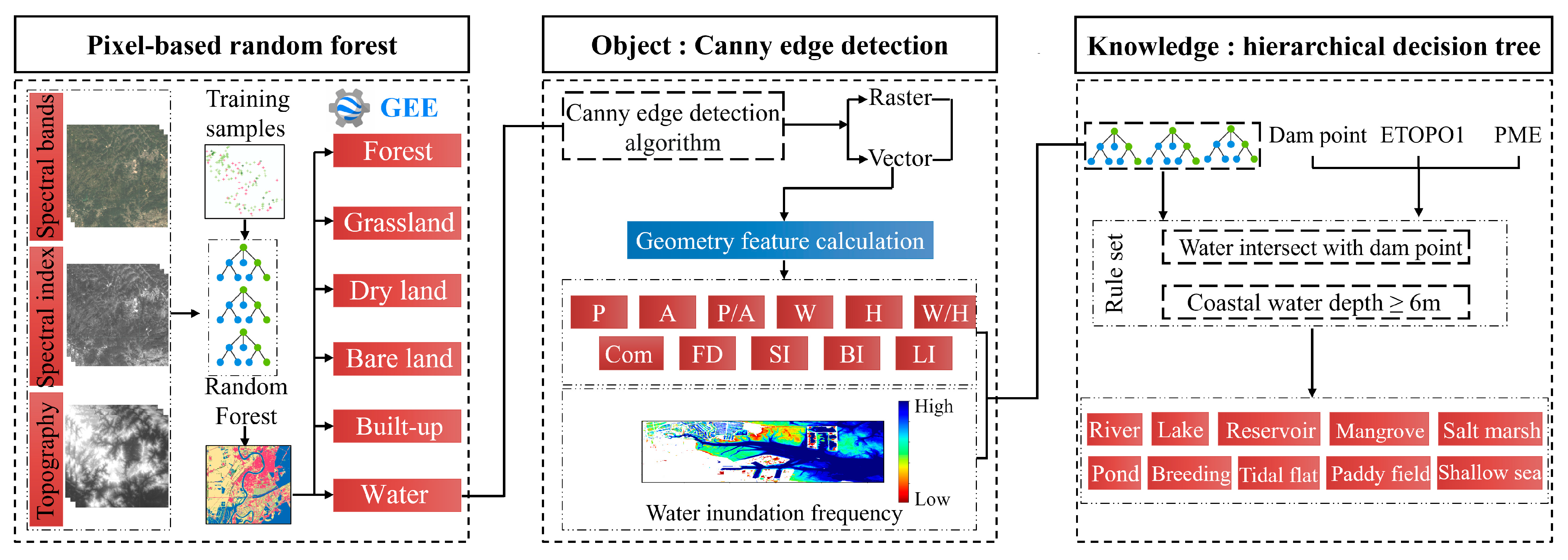
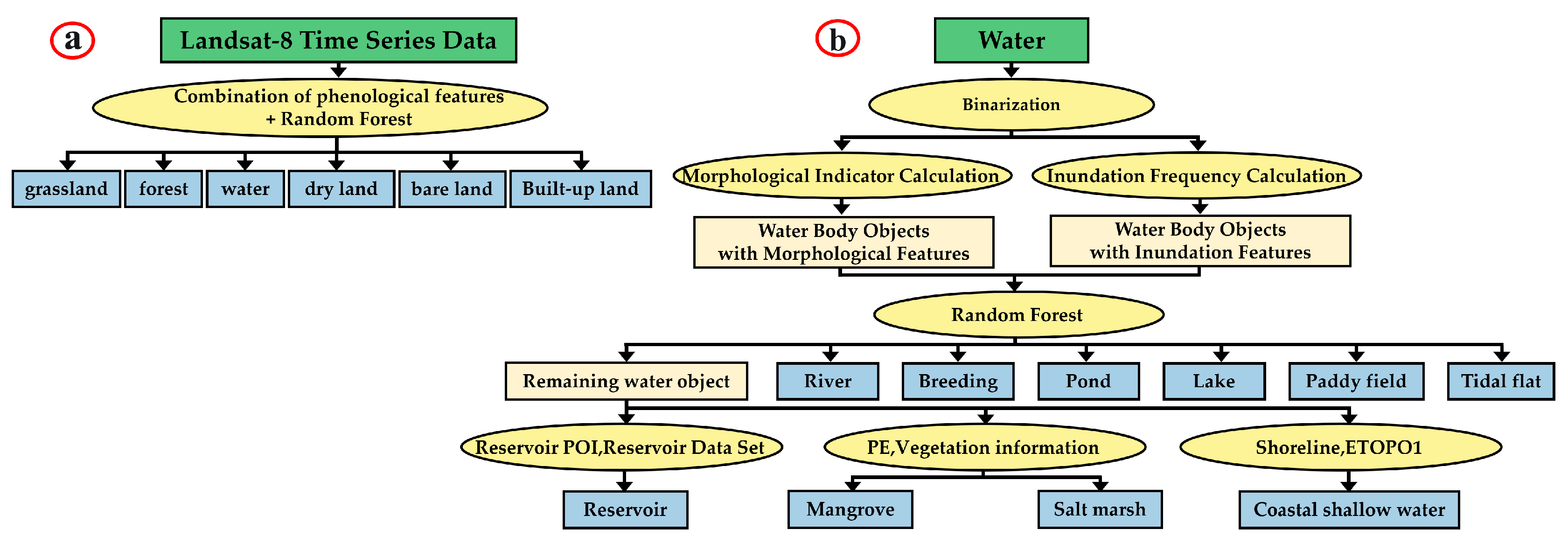
We designed a two-step classification framework that integrates pixel-based Random Forest (RF) classification with object-based hierarchical decision-tree refinement. Here, pixel-based classification refers to Random Forest applied at the pixel level, whereas object-based refinement operates on segmented objects derived from edge detection. A conceptual overview is provided in
Figure 4.
2.5.1. Feature Extraction for Classification
To effectively capture the seasonal variability of wetlands and non-wetlands, we extracted phenology-based features from Landsat-8 imagery spanning January 2019 to December 2021. All data processing and feature extraction, including statistical analyses, were performed using the Google Earth Engine (GEE) cloud computing platform.
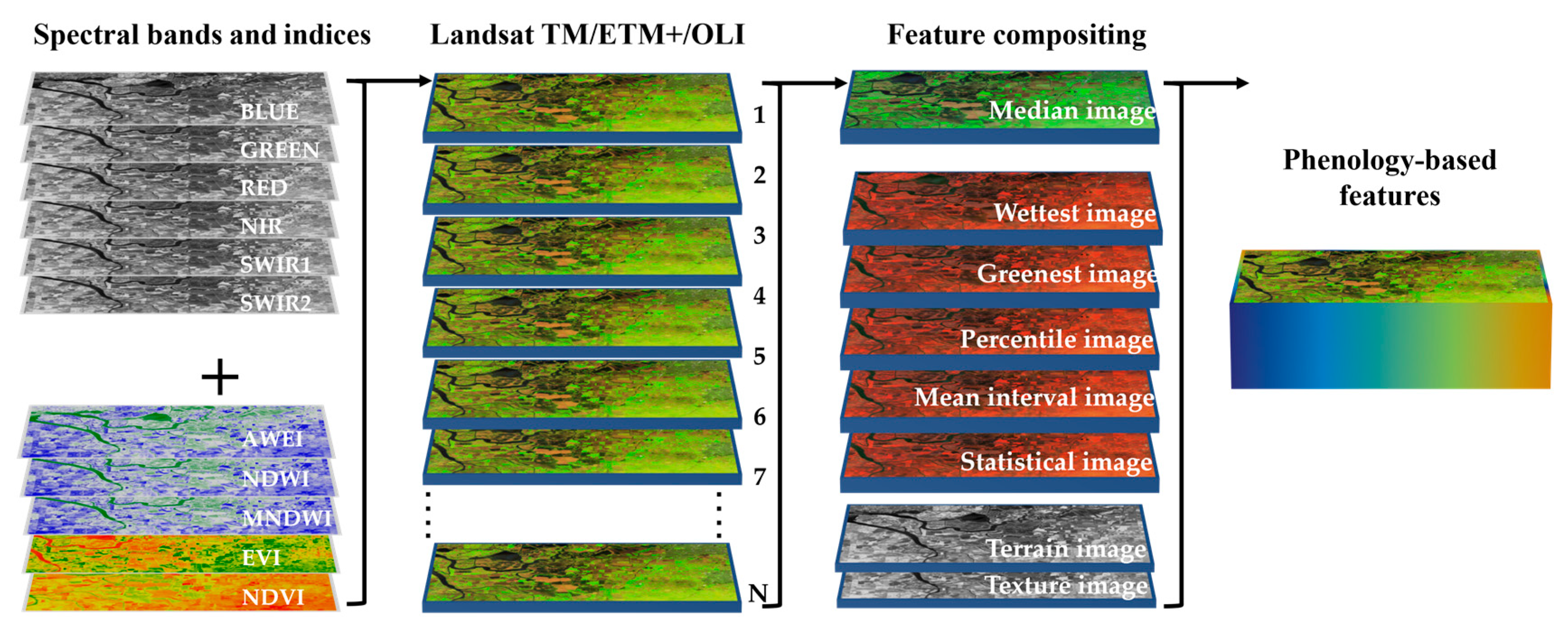
We employed six spectral bands—green, blue, red, NIR, SWIR1, and SWIR2—alongside five spectral indices: the Normalized Difference Vegetation Index (NDVI), Enhanced Vegetation Index (EVI), Normalized Difference Water Index (NDWI), Modified NDWI (MNDWI), and Automatic Water Extraction Index (AWEI). By utilizing GEE, we integrated these bands and indices to generate climatology-based features. These features included median, wettest, and greenest images for the spectral bands, as well as statistical features such as percentiles, mean intervals, and various indices derived from the spectral time series (
Figure 5).
Phenology-based features were derived from multi-temporal Landsat-8 imagery, including representative composites (median, wettest, and greenest images) and a suite of statistical descriptors (percentiles, interval means, and basic descriptive statistics) calculated from spectral index time series using Google Earth Engine [
52,
53]. These statistics were derived from pixel-level histograms generated from the two-year spectral time series, providing a clear representation of the seasonal dynamics in wetland areas.
Mean interval characteristics were computed for different intervals (0–10%, 10–25%, 25–50%, 50–75%, 75–90%, 90–100%, 10–90%, and 25–75%) using the ee.Reducer.intervalMean() function. Additional descriptive statistics, such as maximum, minimum, median, and standard deviation, were calculated from the spectral index time series using the max(), min(), median(), and stdDev() functions. We also derived topographic features, including elevation, slope, and slope aspect, from the SRTM dataset. Texture features were extracted using the gray-level co-occurrence matrix (GLCM) based on the median synthetic NDVI image. In total, 105 feature layers were generated as part of the phenology-based feature set.
To further enhance the accuracy of wetland classification, we selected 11 geometric features, including boundary index, compactness, shape index, fractal dimension, and landscape index. These features were computed using the GEE platform and applied specifically in later stages of object-based classification. Geometric features were not incorporated into the pixel-based Random Forest classification, as they rely on object-level spatial context and were therefore reserved for the object-based refinement stage. In pixel-based classification, each pixel is treated independently without considering the spatial structure, making it unsuitable for incorporating object-level geometric attributes. Therefore, these features were reserved for the object-based refinement stage, where they contribute to the rule-based classification of specific wetland types. A detailed summary of the phenology-based features and their respective roles in wetland classification is presented in
Table 2.
2.5.2. Pixel-Based Random Forest Classification
We implemented a pixel-based Random Forest (RF) classification using phenological features on the Google Earth Engine (GEE) platform. As an ensemble learning algorithm, Random Forest is well suited for handling high-dimensional feature sets in wetland classification tasks [
54]. The key parameters of RF include the number of randomly selected features (mtry) and the number of decision trees (ntree).
The selection of Random Forest parameters followed commonly adopted practices in remote sensing classification. Specifically, mtry was set to the square root of the total number of input feature layers, resulting in a value of 10 [
55], which is a widely used heuristic that balances model diversity and classification stability. The number of trees (ntree) was set to 100 to ensure stable classification performance while maintaining computational efficiency on the Google Earth Engine platform. Previous studies have shown that Random Forest performance is relatively insensitive to moderate changes in these parameters when a sufficient number of trees is used. Therefore, the chosen parameter configuration provides a reasonable trade-off between robustness and computational cost for large-scale wetland mapping.
The RF classifier was used to identify six land types: forest, grassland, built-up area, paddy field, dryland, and bare land. In addition, variable importance derived from the trained Random Forest classifier was used to quantify the contribution of different input features, and the corresponding results are reported in the
Section 3. The focus of this study is on feature design and framework integration rather than exhaustive hyperparameter optimization.
2.5.3. Object-Based Hierarchical Decision Tree Classification
To further refine the six land types identified through RF classification, we developed object-based hierarchical decision trees, incorporating inundation information, geometric features, and auxiliary datasets. The geometric features, including boundary index, shape complexity, shape index, fractal dimension, and landscape index, were calculated on the GEE platform based on the water bodies identified through pixel-based RF classification in
Section 2.5.2. Initially, we extracted binary rasters from the RF classification map, identifying water bodies (1) and non-water bodies (0). The geometric information of water bodies was then calculated using edge detection techniques, and additional geometric characteristics were derived using the morphological evaluation function.
Figure 6 illustrates the structure of the hierarchical decision tree, where the green boxes represent initial input data, the yellow ovals indicate processing steps, the light yellow boxes denote intermediate outputs, and the light blue boxes display the final classification results. It is important to note that coastal deep water was excluded from wetland classification and categorized as background.
2.6. Processing After Classification
This post-classification step was designed as an auxiliary refinement to the pixel-based Random Forest results rather than a primary classification process. To further improve the accuracy of wetland mapping, post-classification refinement was applied to both the pixel-level outputs and the object-based classification results within the two-step framework.
Misclassifications in the pixel-level Random Forest results were corrected through manual inspection by comparing the classification outputs with high-resolution imagery. This step was used to identify and correct obvious errors and to improve the overall reliability of the land-cover maps.
Following the object-based classification, a series of rule-based refinements was applied to resolve ambiguities among spectrally similar water-related classes. Specifically, water bodies with an area smaller than 0.01 km2 that intersected aquaculture ponds within a 30 m buffer were reclassified as aquaculture ponds, while small aquaculture ponds (<0.01 km2) intersecting rivers were reclassified as rivers. In addition, unclassified water bodies were cross-referenced with the Global River Widths from Landsat (GRWL) dataset to identify river features.
Manual interpretation using high-resolution imagery was applied only as a final step to resolve residual ambiguities that could not be addressed through rule-based refinement. Manual corrections accounted for a limited proportion of classified objects and were primarily confined to complex boundary areas. This combination of systematic rule-based refinement and limited manual adjustment helped resolve ambiguities in complex and fragmented wetland environments.
2.7. Accuracy Assessment
This study utilized 10 m resolution Sentinel-2 MSI images, acquired between 1 January 2019 and 31 December 2021, as reference data for accuracy assessment. Validation samples were generated using a combination of stratified random sampling and visual interpretation. Specifically, stratified random points were first created in ArcGIS 10.4 and subsequently interpreted using Sentinel-2 MSI imagery, resulting in a total of 5047 reference sample points.
Based on these reference samples and the classification results, a confusion matrix was constructed to calculate Producer’s Accuracy (PA), User’s Accuracy (UA), Overall Accuracy (OA), and the Kappa coefficient following standard definitions. The reported accuracy metrics reflect classification performance under this validation framework.
3. Results
3.1. Classification Results of Pixel-Level RF Algorithm
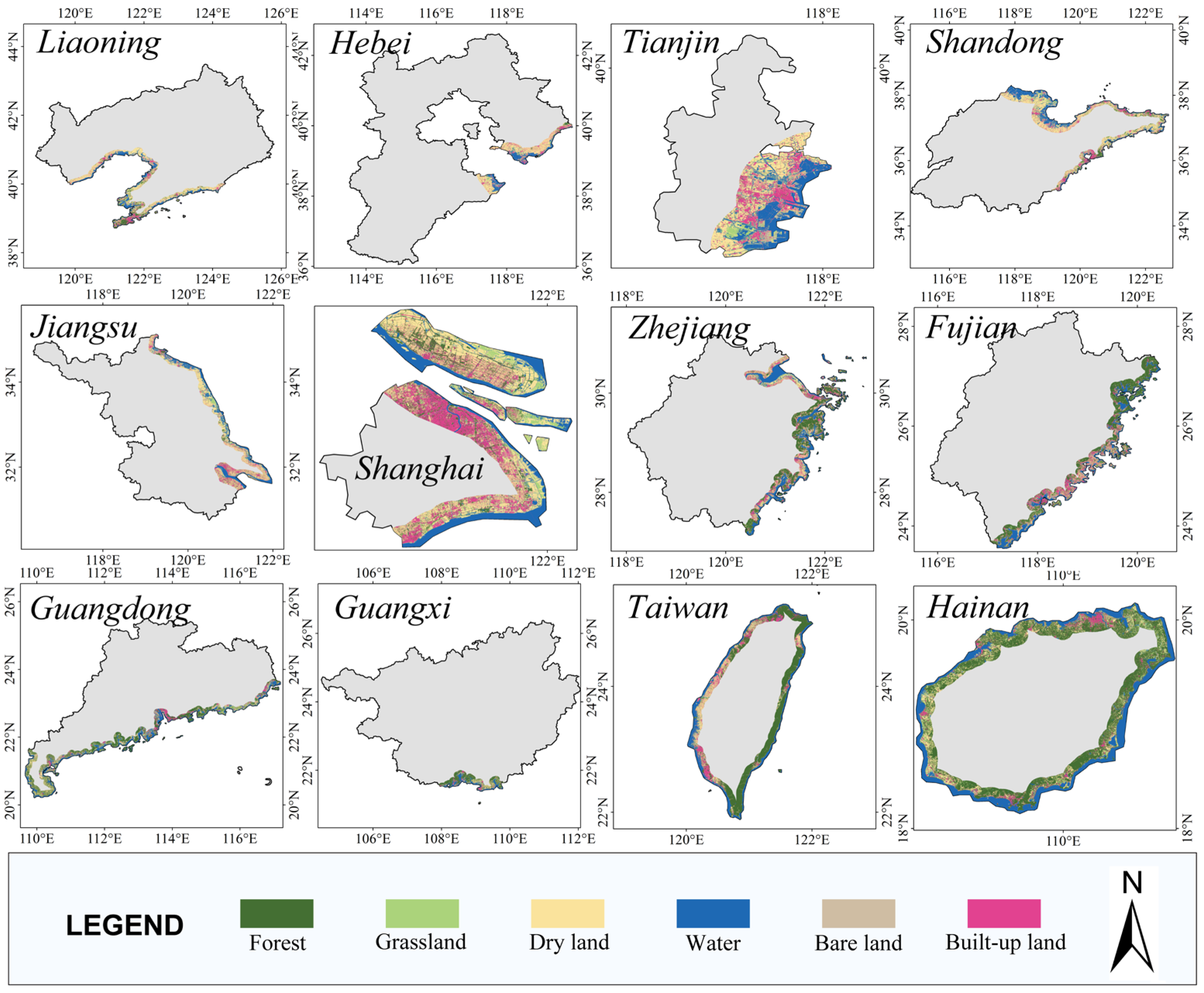
The preliminary classification results are shown in
Figure 7, which illustrates the spatial distribution of major land cover types in China’s coastal provinces in 2020. Guangdong, Fujian, and Hainan exhibited extensive forest cover, with forest areas of 9515 km
2, 7313 km
2, and 5799 km
2, respectively, indicating high forest coverage. Shandong had the largest water area, reaching 6528 km
2, highlighting its rich aquatic ecosystems. Shandong was also the province with the largest cropland area (10,291 km
2), underscoring its importance as one of China’s major agricultural regions.
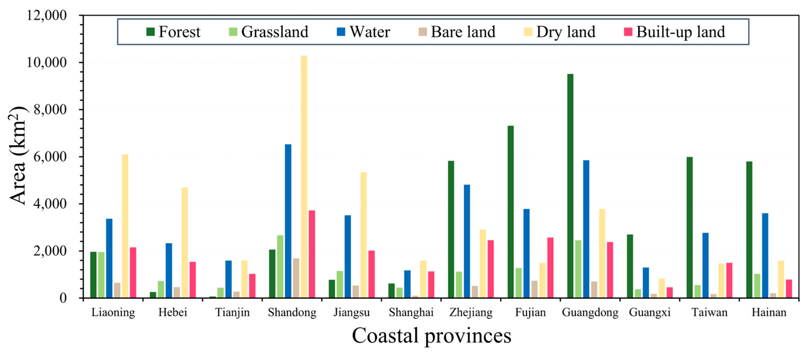
The area statistics for the preliminary RF classification are summarized in
Figure 8 and
Table 3. Shandong showed the highest degree of urbanization, with built-up land covering 3719 km
2, followed by Guangdong and Liaoning, reflecting a high level of urban development in these provinces. Grassland areas in Shandong and Liaoning were also notable, measuring 2659 km
2 and 1954 km
2, respectively, indicating substantial pastoral landscapes. Although bare land was not extensive overall, it was particularly prominent in Shandong (1685 km
2) and Liaoning (643 km
2), which may reflect natural rocky coastlines or human-induced disturbances such as mining.
These preliminary results deepen our understanding of the distribution of major land cover types in China’s coastal regions and provide a basis for subsequent object-based refinement. Together, they offer essential support for ecological monitoring, sustainable development, and environmental management in coastal zones.
The accuracy assessment of the preliminary RF-based classification indicates good overall performance, with an overall accuracy (OA) of 84.83% and a Kappa coefficient of 0.8178, demonstrating a high level of agreement with the reference data (
Table 4). However, some misclassification remains due to spectral and surface feature similarities among different land cover types.
For water bodies, both user’s accuracy (UA, 92.57%) and producer’s accuracy (PA, 93.31%) were high, yet certain lakes that had partially dried up were misclassified as bare land, and water surfaces with overlying structures were sometimes identified as built-up land. Forest classification also exhibited high accuracy (UA = 86.99%, PA = 93.88%), but sparse forests with low canopy cover were occasionally confused with grassland, and orchards with regularly spaced trees were sometimes misclassified as cropland—errors commonly reported in forest mapping.
Grassland suffered from higher confusion with cropland and dryland due to similarities in vegetation type and coverage, particularly when using medium-resolution imagery. Its UA and PA were 71.68% and 75.36%, respectively, indicating frequent misclassification in transitional zones. Bare land (UA = 86.55%, PA = 82.73%) was sometimes confused with built-up land because exposed surfaces share similar spectral characteristics; conversely, unpaved open areas within built-up regions were occasionally labeled as bare land. Dryland showed similar issues, especially at early crop growth stages or when vegetation was sparse, increasing confusion with grassland. For cropland (dry land), UA was 81.73% and PA was 71.03%, reflecting the challenges of distinguishing it from grassland in areas with mixed or transitional vegetation conditions.
3.2. Feature Contribution and Variable Importance
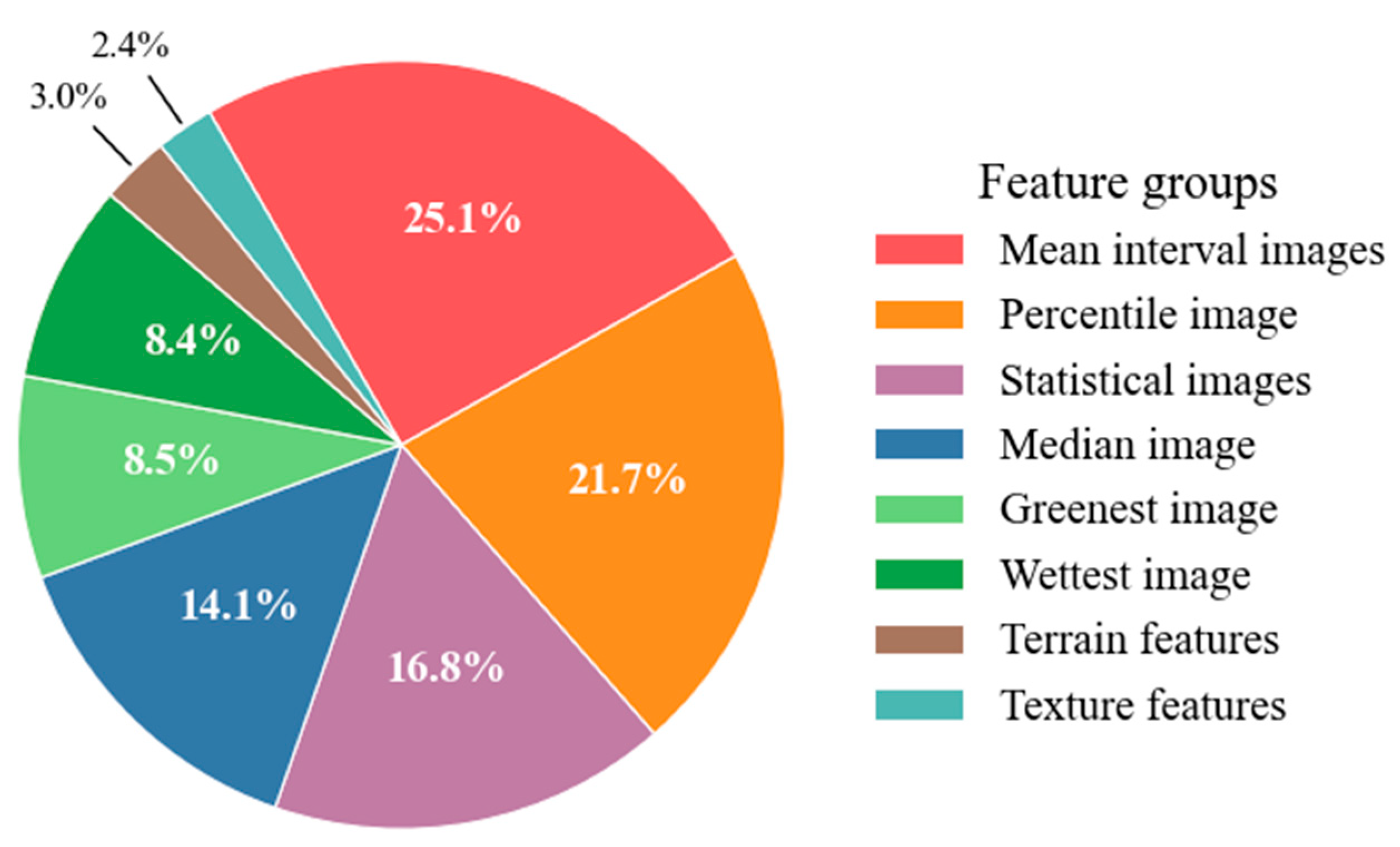
To evaluate the contribution of different input features, a variable importance analysis was conducted using the Random Forest classifier. Given the large number of input variables, features were grouped according to their temporal compositing logic and information content, including median image, wettest image, greenest image, percentile image, mean interval images, statistical images, as well as terrain and texture features. Aggregated (summed) importance scores were calculated for each feature group to reflect their overall contribution to classification performance (
Figure 9).
The results indicate that time-series-related features dominate the model contribution. Mean interval images (25.1%) and percentile images (21.7%) together account for nearly half of the total importance, highlighting the critical role of temporal variability and distributional characteristics in coastal wetland classification. Statistical images (16.8%) and median composites (14.1%) also contribute substantially, suggesting that both temporal dispersion and stable background spectral information are important for robust mapping. In contrast, features derived from representative phenological states, including greenest (8.5%) and wettest (8.4%) images, play a secondary but non-negligible role, particularly in distinguishing vegetation- and water-related wetland types. Terrain (3%) and texture features (2.4%) show relatively lower contributions, indicating that they primarily serve as auxiliary constraints in complex spatial contexts. Overall, these findings support the feature design of the proposed framework and emphasize the dominant influence of time-series information in coastal wetland mapping.
3.3. Ablation and Cross-Validation Results
To further assess the robustness and reliability of the proposed classification framework, ablation and cross-validation experiments were conducted.
To evaluate the contribution of key feature groups in the proposed framework, a simple ablation experiment was conducted, and the results are summarized in
Table 5. Removing mean interval features led to a notable decrease in overall accuracy and Kappa coefficient, while excluding texture features also resulted in performance degradation, indicating that both feature groups contribute to classification performance.
In addition, a five-fold cross-validation was applied to assess model robustness. As shown in
Table 6, the classifier achieved a mean overall accuracy of 89.64% with a standard deviation of 1.1%, and a mean Kappa coefficient of 0.892 ± 0.08, demonstrating stable performance across different training–validation splits.
3.4. Detailed Classification Results of Wetland Types
To evaluate the performance of the object-based classification in identifying wetland types across coastal China, we conducted an accuracy assessment of the 2020 detailed classification results. The model performed well, with an overall accuracy (OA) of 89.76% and a Kappa coefficient of 0.891, indicating a high level of consistency with the reference data (
Table 7).
Table 5 also reveals notable differences in accuracy among wetland types, highlighting the relative difficulty of distinguishing certain categories.
Wetland and land-cover types such as shallow sea, forest, and built-up land achieved the highest accuracies, with both PA and UA exceeding 90%, indicating strong separability. In contrast, paddy field, dry land, river, and pond categories exhibited relatively lower accuracies. For example, the PA of paddy fields was only 71.51%, suggesting frequent confusion with other land covers that share similar spectral and structural characteristics.
The main sources of misclassification include: (1) rivers during the dry season may be confused with ponds due to lower water levels; (2) paddy fields during irrigation may resemble water-covered tidal flats in satellite imagery; (3) inactive aquaculture ponds may visually resemble dried croplands; (4) lakes and reservoirs, despite relatively high accuracy, are occasionally misclassified due to similar water body characteristics and shapes, especially when reservoirs exhibit more regular geometry; and (5) distinguishing between shallow sea and lakes or reservoirs at the water edges is challenging when water depth and boundary conditions are similar.
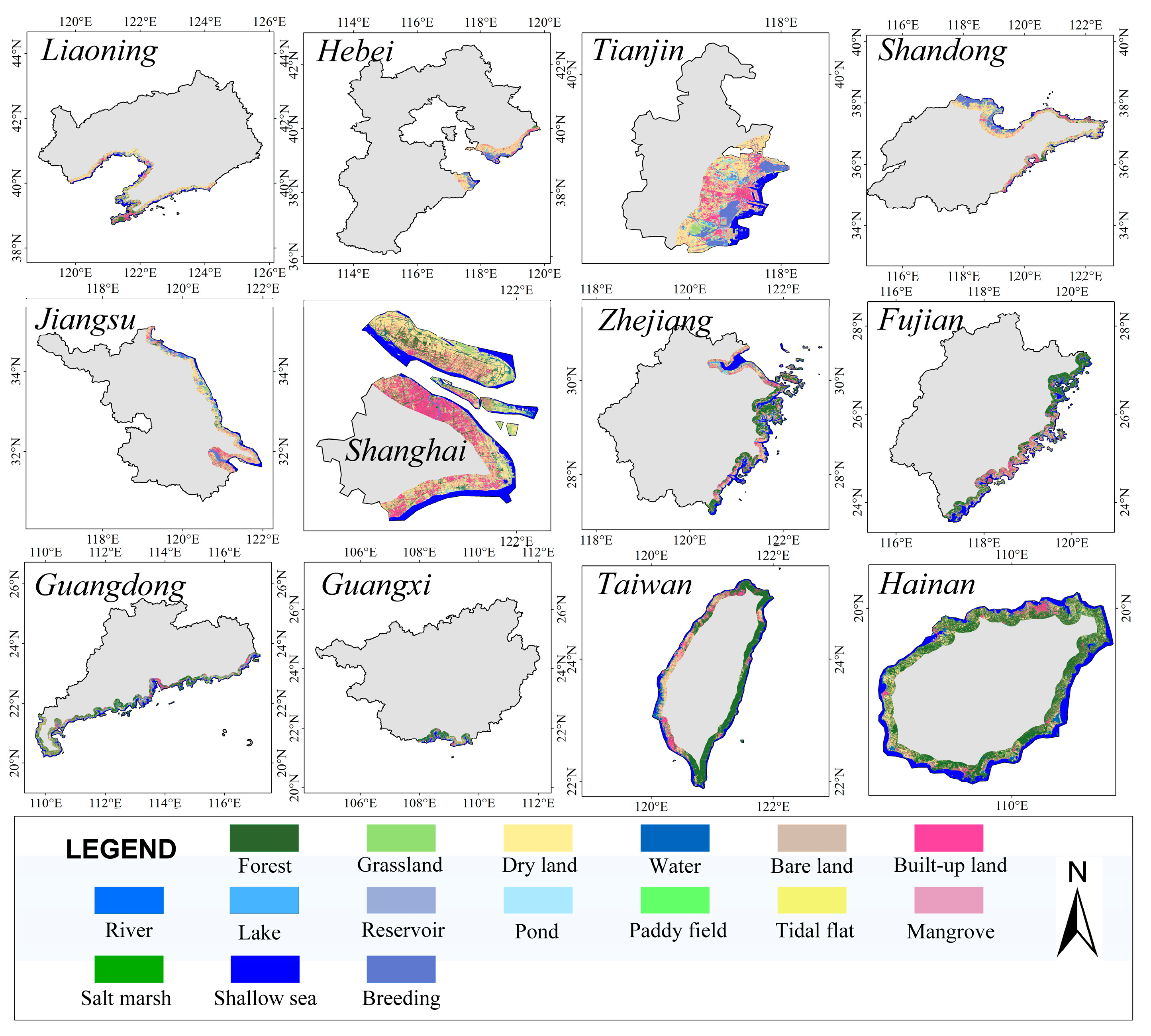
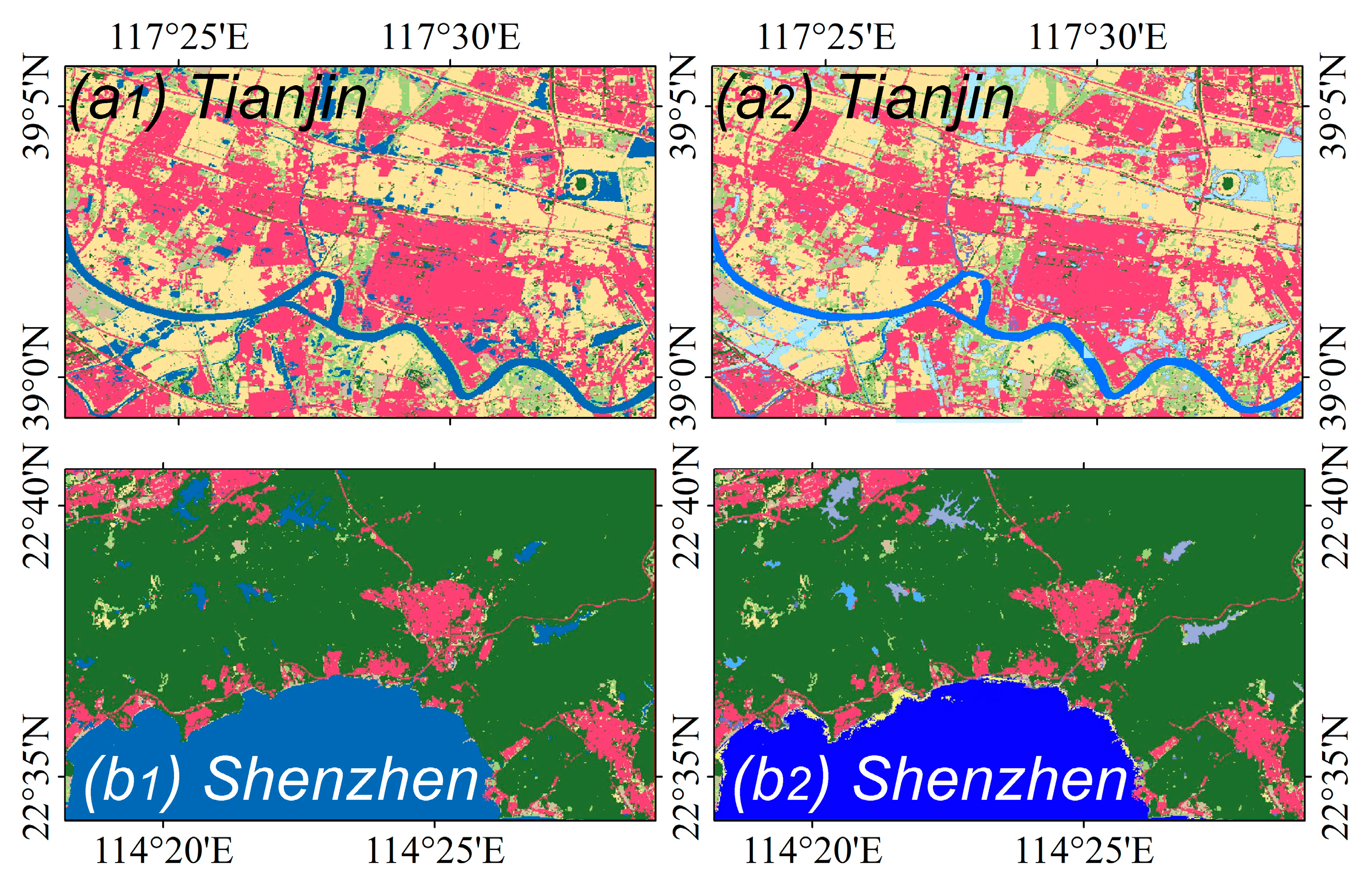
To provide a clearer understanding of the classification results,
Figure 10 illustrates the spatial distribution of wetland types across the 12 coastal provinces of China.
Figure 11 presents the detailed classification outcomes in three representative regions—Shenzhen, Dongying, and Dalian, selected from the southern, central, and northern coastal zones, respectively—highlighting regional classification characteristics and spatial patterns.
3.5. Comparative Analysis with the FCS30 Dataset
3.5.1. Comparison of Mangrove Classification Results with the FCS30 Dataset
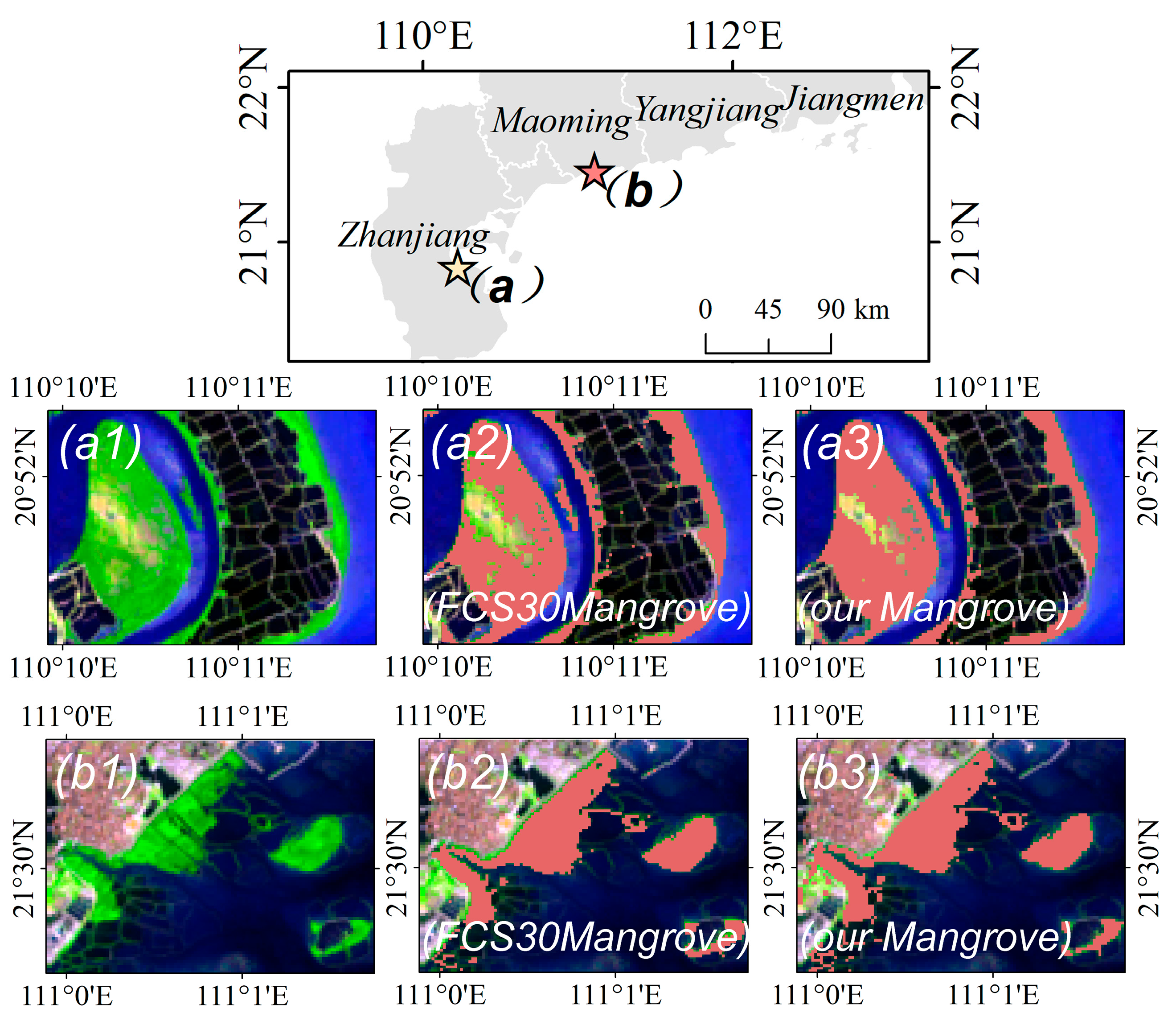
Statistical analysis showed that the spatial distribution of mangroves derived in this study was largely consistent with that of the FCS30 dataset. To further examine spatial consistency and local discrepancies, two representative regions—Zhanjiang and Maoming—were selected for detailed comparison (
Figure 12). In both regions, the spatial patterns of mangroves in our classification and FCS30 were broadly similar, capturing the characteristic belt-shaped distribution along estuaries and bays. The high degree of overlap indicates that the proposed two-step framework can accurately delineate major mangrove zones.
Nevertheless, slight discrepancies appeared in narrow coastal strips and fragmented patches. These differences are mainly attributable to the classification methods and data sources. In our study, mangroves were mapped using a two-step framework that combines pixel-based RF with object-based hierarchical decision trees based solely on Landsat-8 imagery. In contrast, FCS30 was produced using a deep-learning framework integrating multi-source data (Landsat-8, Sentinel-2, MODIS). As a result, FCS30 mangrove patches tend to be smoother and more generalized, whereas our classification preserves fine-scale details and boundary heterogeneity in natural mangrove stands.
3.5.2. Comparison of Salt Marsh Classification Results with the FCS30 Dataset
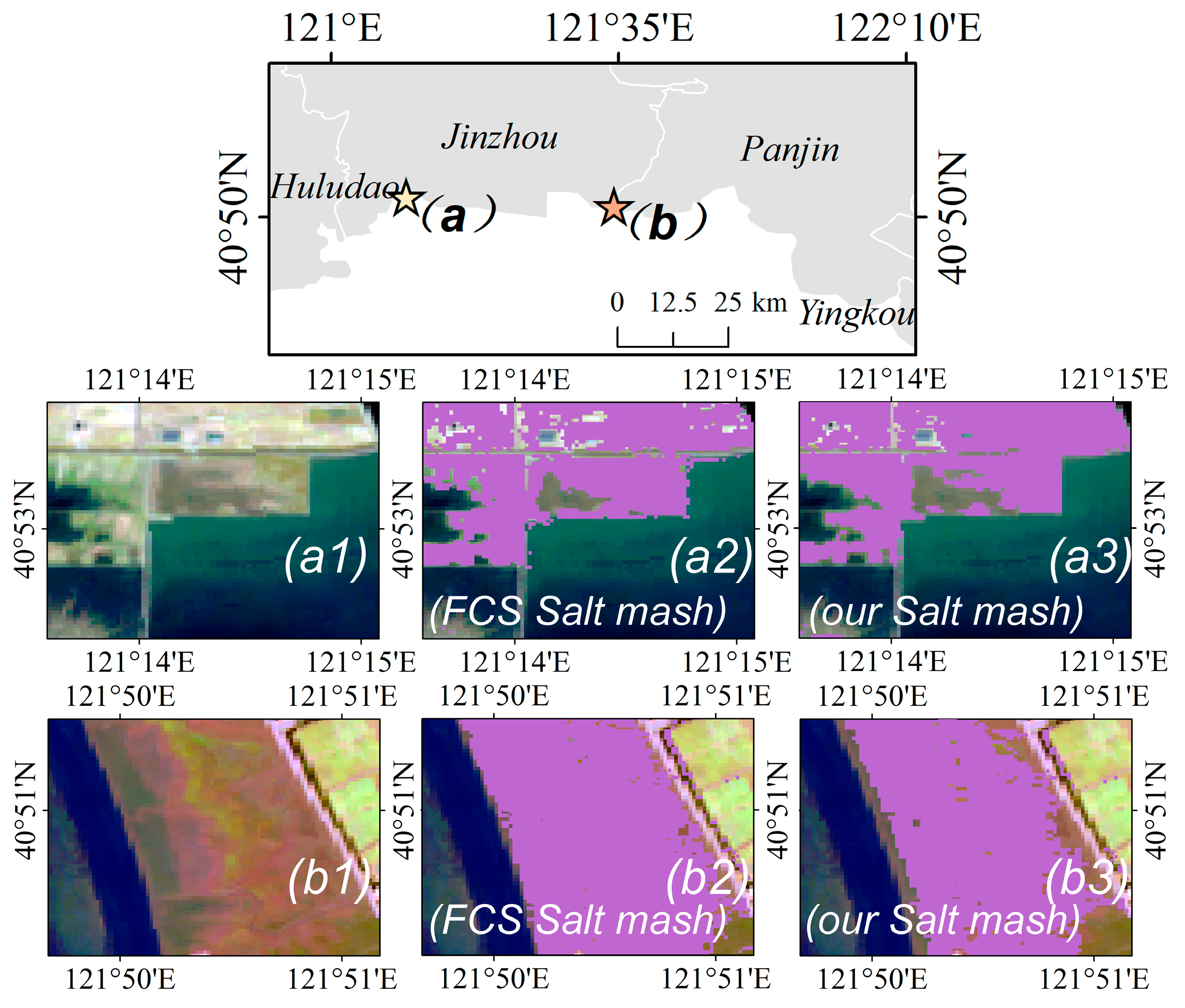
Similarly, the spatial distribution of salt marshes derived in this study was generally consistent with that of the FCS30 dataset. To further assess spatial consistency and local discrepancies, two representative regions—Jinzhou and Panjin—were selected for detailed comparison (
Figure 13). Both datasets captured the extensive distribution of salt marshes along the Bohai coastal plain, showing comparable boundaries and similar patterns of vegetation expansion into tidal flats. Minor discrepancies occurred in narrow or fragmented transition zones between salt marsh and tidal flat, where mixed spectral signals led to partial misclassification.
These inconsistencies can be attributed to differences in classification approaches, data sources, and temporal coverage. Our study employs a two-step classification framework based on 30 m Landsat-8 imagery, while the FCS30 dataset is generated by a deep-learning model integrating multiple sensors, including Landsat-8, Sentinel-2, and MODIS. The higher temporal frequency of FCS30 tends to smooth seasonal spectral variations, whereas our classification better preserves fine-scale structural details and patch boundaries of salt marsh vegetation.
3.6. Area Analysis of Detailed Classification Results for Wetland Types in Coastal Provinces of China
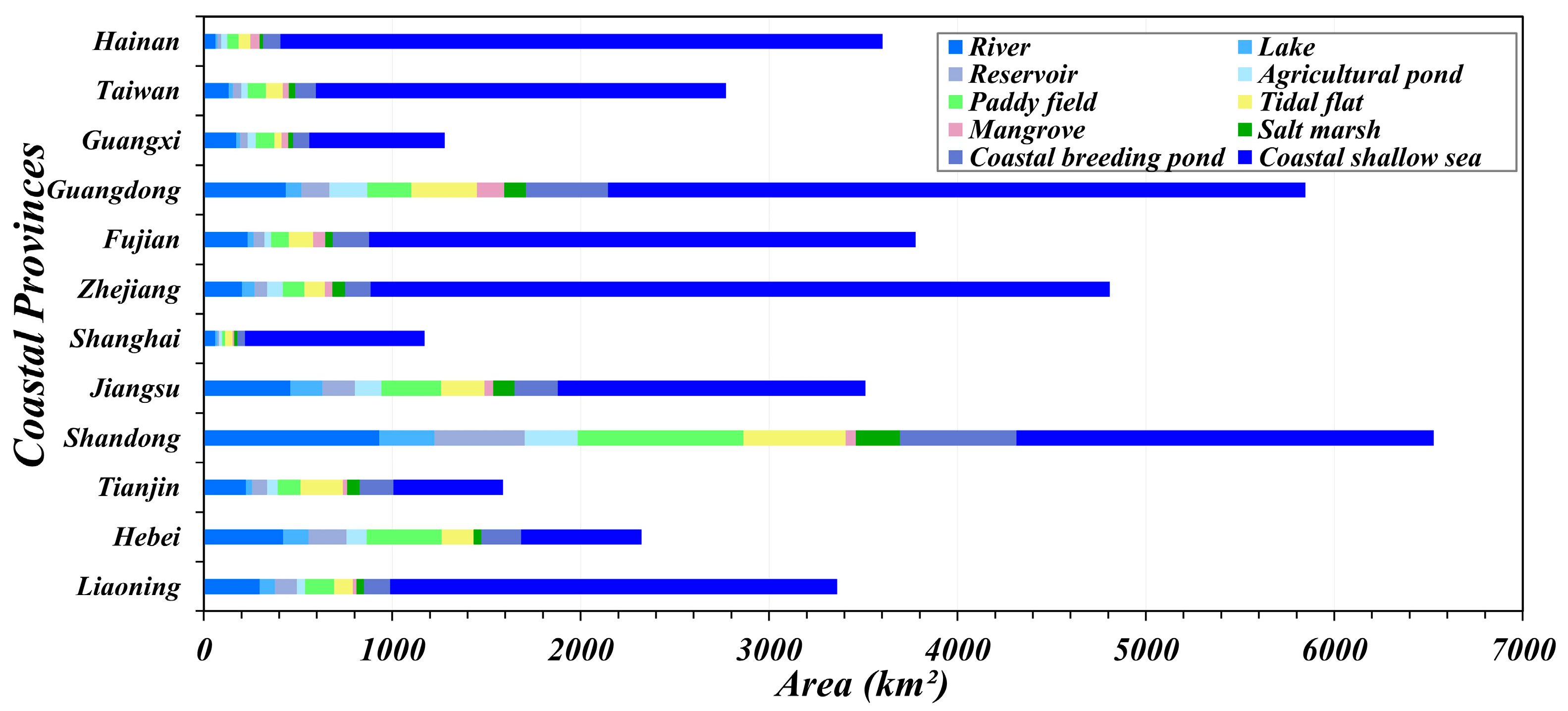
The detailed classification of wetland types across China’s coastal provinces reveals a rich diversity of ecosystems, ranging from large river and lake systems to specialized habitats such as mangroves and salt marshes. Northern provinces such as Liaoning and Hebei contain extensive coastal and riverine systems, along with substantial paddy field areas, reflecting strong linkages between aquatic environments and agricultural production. Tianjin is characterized by extensive tidal flats, consistent with its unique coastal geomorphology. The spatial differences in wetland area among coastal provinces are further illustrated by the area statistics derived from the two-step classification results (
Figure 14).
Table 8 summarizes the area statistics of detailed wetland types. In southern provinces such as Zhejiang, Fujian, and Guangdong, coastal wetlands are particularly prominent. For example, coastal shallow waters in Zhejiang cover more than 3900 km
2, while Guangdong exhibits diverse wetland types with extensive coastal breeding ponds and shallow seas, reflecting a highly productive and intensively utilized coastal environment.
The outlying regions of Guangxi, Taiwan, and Hainan also play crucial roles in maintaining coastal biodiversity. In particular, Hainan has the largest extent of coastal shallow sea (3195 km2), underlining its ecological importance for marine and coastal ecosystems. This comprehensive area analysis highlights the ecological significance of China’s coastal wetlands and underscores the need for targeted conservation and sustainable management strategies to protect these vital resources.
4. Discussion
4.1. Advancements in Wetland Monitoring and Classification Techniques
The two-step classification method employed in this study provides an efficient and accurate framework for fine-scale coastal wetland mapping in China, with potential applicability to other coastal regions following regional calibration and validation. By integrating pixel-based Random Forest algorithms with object-based hierarchical decision trees, the approach effectively addresses the spectral similarity among wetland types that often constrains traditional classification methods. This framework is well suited to large-scale, long-term ecological monitoring based on remote sensing data.
A key strength of the method lies in its use of Landsat-8 time-series imagery in combination with the computational capabilities of the Google Earth Engine (GEE) platform. This design allows the method to capture the seasonal and interannual dynamics of wetland ecosystems, thereby improving the separability of spectrally similar classes—especially vulnerable wetland types such as tidal flats, mangroves, and salt marshes. These ecosystems are frequently underrepresented or misclassified in conventional land-cover products. Enhanced classification precision can support improved detection of habitat degradation and provide a more reliable spatial basis for delineation conservation zones and informed adaptive management. These improvements are relevant for informing assessments related to national and international wetland conservation frameworks, such as the Ramsar Convention.
Beyond its technical contributions, the approach developed here provides valuable scientific support for wetland conservation and restoration. The refined wetland maps generated by this method serve as important inputs for ecological modeling, habitat suitability assessments, and the planning of protected areas. By improving both the spatial and thematic accuracy of wetland classifications, the method can assist policymakers and managers in assessing ecological conditions, identifying conservation priorities, and supporting the development of management strategies.
4.2. Ecological Significance of High-Resolution Wetland Classification
Accurate, fine-scale classification of wetland types is essential for biodiversity conservation and the sustainable management of ecosystem services, particularly in ecologically sensitive and heavily human-impacted coastal zones. Traditional land-cover datasets often lack the spatial resolution or thematic detail needed to represent small, fragmented, or spectrally similar wetland features. In contrast, the two-step classification approach proposed in this study—combining pixel-based Random Forest with object-based refinement—achieves improved spatial accuracy and delineation of detailed wetland subtypes.
Our results demonstrate that high-resolution classification improves the detection of ecologically critical wetland types, including salt marshes, aquaculture ponds, tidal flats, and rivers. These habitats provide diverse and irreplaceable ecosystem services: salt marshes and tidal flats serve as key stopover and foraging sites for migratory birds; aquaculture ponds and shallow rivers support nursery habitats for aquatic organisms; and vegetated wetlands mitigate storm surges and coastal erosion by dissipating wave energy. In addition, detailed wetland maps form an important dataset for ecological modeling, habitat suitability analysis, and policy development related to protected area designation and restoration planning.
The spatial patterns revealed by the detailed classification further enhance ecological understanding at the regional scale. For example, northern provinces such as Liaoning and Hebei contain extensive riverine and coastal wetlands, often closely associated with agricultural zones dominated by paddy fields. In contrast, southern provinces including Zhejiang, Fujian, and Guangdong exhibit large areas of shallow coastal waters and breeding ponds, reflecting both high wetland productivity and intensive human utilization. Outlying regions such as Guangxi, Taiwan, and Hainan also play important roles in maintaining regional biodiversity—particularly Hainan, which has the largest area of coastal shallow seas (3195 km2). These regional differences underscore the importance of tailoring conservation and management strategies to local ecological contexts rather than adopting uniform policies across all coastal regions.
In summary, integrating high-resolution classification with a robust classification logic improves not only thematic accuracy but also the practical utility of land-cover data for biodiversity and ecosystem-service assessments. Our findings highlight the potential of data-driven, high-resolution mapping to support science-based wetland conservation and sustainable land use strategies in coastal regions.
4.3. Challenges, Uncertainties, and Future Directions
Despite the overall robustness and satisfactory performance of the proposed classification framework, several challenges and sources of uncertainty should be acknowledged. First, the generation of training samples relied on a combination of semi-automatic extraction and manual visual interpretation. Although careful screening was applied to improve label reliability, this process may introduce a degree of subjectivity and spatial dependence, potentially affecting sample independence and reproducibility, particularly in heterogeneous coastal environments. In addition, uneven sample sizes among different wetland classes may also contribute to class-specific uncertainty in the accuracy assessment.
Second, the object-based refinement step incorporated a set of rule-based decisions and limited manual corrections to resolve ambiguities among spectrally similar water-related classes, such as rivers, reservoirs, ponds, and paddy fields. While this refinement improves local classification accuracy, it reduces full automation and may introduce additional subjectivity. The extent of manual intervention was therefore quantified, and its potential influence on the classification results should be considered when interpreting the mapped wetland patterns.
Third, uncertainties also arise from the inherent temporal variability of coastal environments and from differences between the Landsat imagery used for classification and the Sentinel-2 imagery used for accuracy assessment. The integration of multi-temporal imagery across different acquisition dates may be influenced by tidal phase differences, phenological shifts, and mixed pixels in transitional zones, particularly in estuarine and intertidal areas. These factors can contribute to class confusion and temporal mismatches between nominal classification periods and actual land cover conditions.
Finally, although the ablation experiments and five-fold cross-validation demonstrate the robustness and stability of the proposed framework, its transferability across broader geographic contexts remains to be further evaluated. The current study focuses on China’s coastal provinces, and future work could explore region-specific calibration strategies and independent spatial validation before applying the framework to other coastal regions with different environmental and socio-economic settings.
5. Conclusions
This study developed a two-step wetland classification framework that integrates pixel-based Random Forest classification with object-based hierarchical refinement to generate a high-resolution wetland map for China’s coastal provinces. By leveraging multi-temporal Landsat imagery and the computational capabilities of the Google Earth Engine platform, the proposed approach effectively addresses challenges associated with spectral similarity, seasonal variability, and class confusion in complex coastal environments.
The results demonstrate that time-series-derived features play a dominant role in coastal wetland classification, while the combination of pixel-level learning and object-based refinement improves the discrimination of ecologically important and spectrally complex wetland types, such as tidal flats and mangroves. Variable importance analysis, ablation experiments, and five-fold cross-validation collectively confirm the robustness and stability of the proposed framework.
The resulting wetland map reveals pronounced spatial heterogeneity in wetland composition across China’s coastal provinces and provides a consistent basis for analyzing wetland distribution patterns and area statistics at the provincial scale. These findings offer valuable scientific support for coastal wetland monitoring, assessment, and management within the Chinese coastal context.
Nevertheless, the applicability of the proposed framework is subject to certain limitations related to training sample generation, manual refinement, and temporal variability inherent to coastal systems. As discussed, regional calibration and independent validation would be required before transferring the framework to other geographic contexts with different environmental and socio-economic conditions.
Overall, this study highlights the potential of combining time-series remote sensing data with hybrid classification strategies for detailed coastal wetland mapping. The framework provides a flexible and reproducible foundation for future studies aimed at improving long-term coastal wetland monitoring and supporting evidence-based conservation and management efforts.
