Funding
This research was funded by the Shandong Province Key R&D Program (Competitive Innovation Platform) Project, Grant No. 2024CXPT101, “Research on Key Technologies for Monitoring and Evaluation of Ecological Restoration Effect of Mines in the Yellow River Basin (Shandong Section)”, the Qingdao Science and Technology for the Benefit of People Project, Grant No. 25-1-5-xdny-12-nsh, “High-Standard Farmland Integrated Sky–Aerial–Ground Intelligent Supervision Technology and Application”, the China Postdoctoral Science Foundation (76th General Program), Grant No. 2024M761845, “Airborne GNSS-IR High-Precision Sea-Surface Height Inversion Methods and Model”, the Open Fund of the Key Laboratory of Marine Environmental Survey Technology and Application, Ministry of Natural Resources, Grant No. MESTA-2024-B001, “Spatiotemporally Intelligent Sea-Surface Wind-Speed Retrieval via Multi-source Collaborative Spaceborne GNSS-R Sensing”, the Qingdao Natural Science Foundation (Young Scientists Program), Grant No. 25-1-1-54-zyyd-jch, “Multi-source-Collaborative Spaceborne GNSS-R Sea-Surface Salinity Inversion Methods and Model”, the Shandong Provincial Postdoctoral Innovation Project, Grant No. SDCX-ZG-202502046, “Global Sea-Surface Salinity Inversion via Multi-source Collaborative Spaceborne GNSS-R”, and the National Program for Funding Postdoctoral Researchers (Category B), Grant No. GZB20250067, “Global Sea-Surface Salinity Inversion via Multi-source Collaborative Spaceborne GNSS-R”.
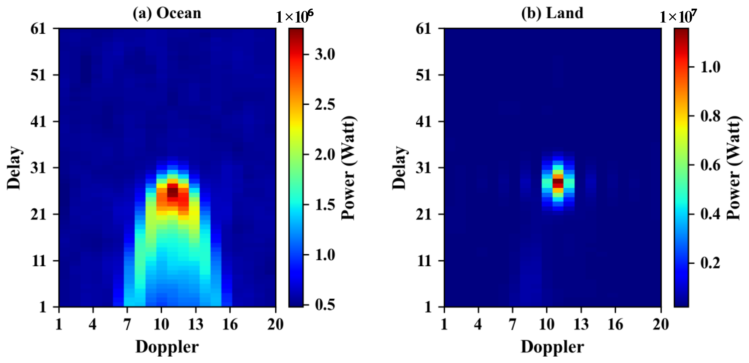
Figure 1.
TM-1 Delay–Doppler Maps (DDMs): (a) ocean and (b) land.
Figure 1.
TM-1 Delay–Doppler Maps (DDMs): (a) ocean and (b) land.
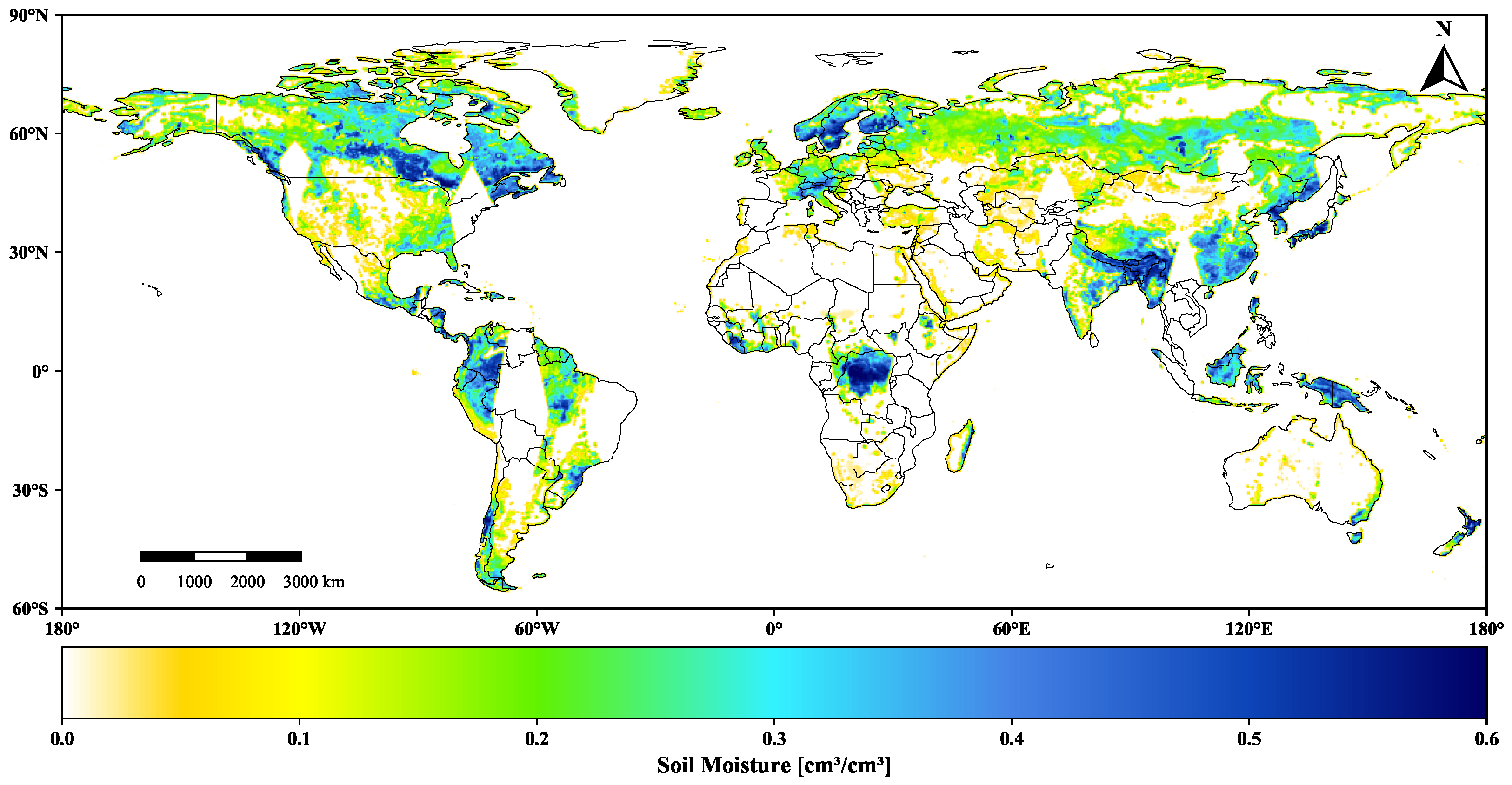
Figure 2.
Spatial distribution of SMAP soil moisture on 28 August 2023. The color bar below the map represents the soil moisture values and their corresponding color range.
Figure 2.
Spatial distribution of SMAP soil moisture on 28 August 2023. The color bar below the map represents the soil moisture values and their corresponding color range.
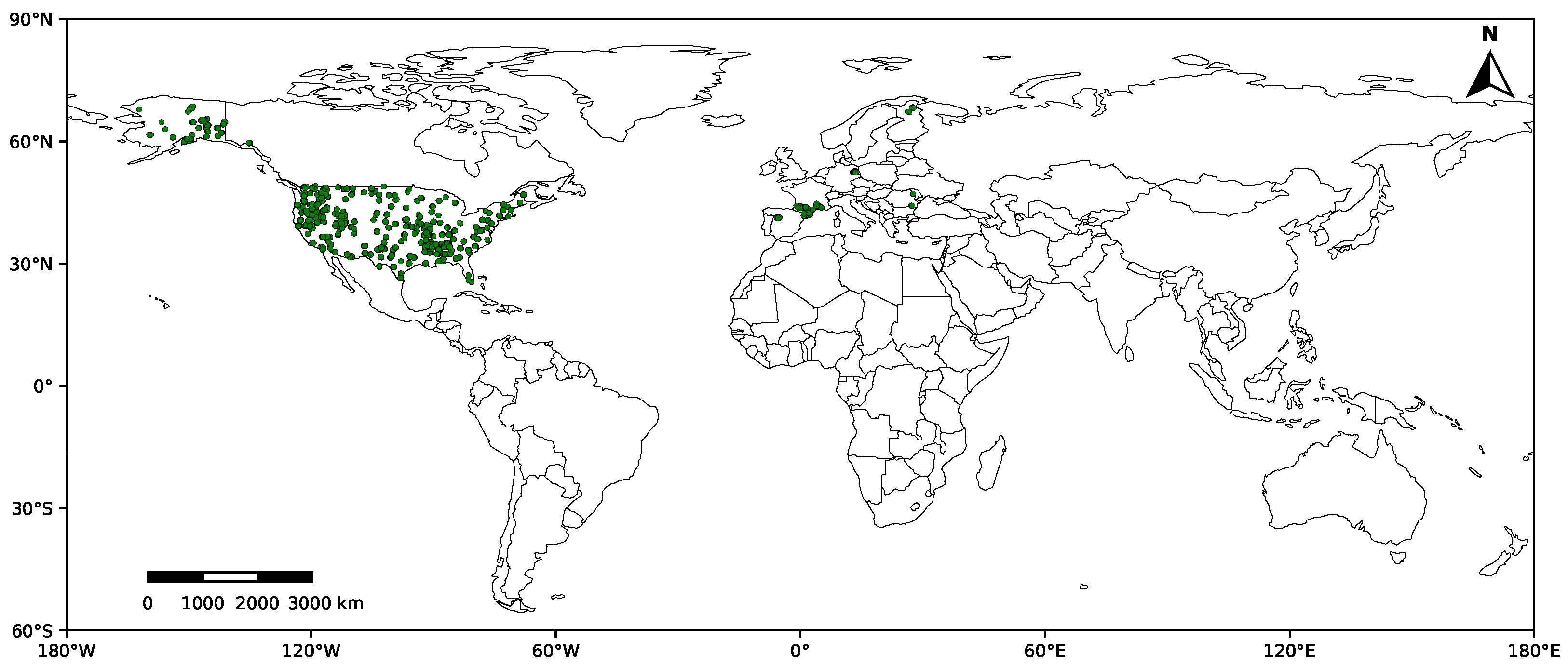
Figure 3.
Spatial distribution of ISMN in in situ stations. Green dots represent the ISMN surface soil moisture observation sites (0–5 cm) used for independent validation in this study.
Figure 3.
Spatial distribution of ISMN in in situ stations. Green dots represent the ISMN surface soil moisture observation sites (0–5 cm) used for independent validation in this study.
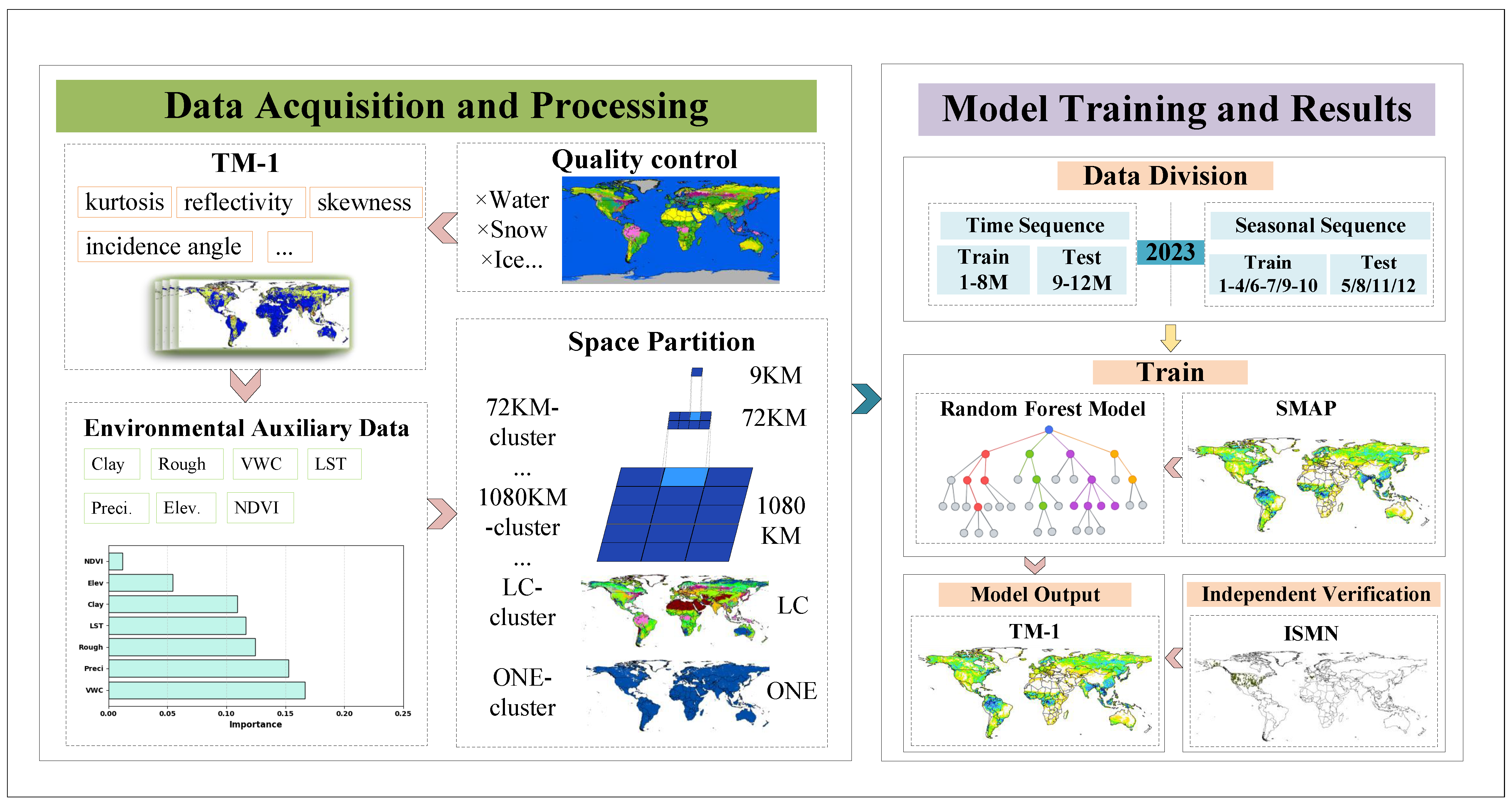
Figure 4.
Overall methodological framework. “M” denotes month in 2023; under the time-sequence split, 1–8M (January–August) are used for training and 9–12M (September–December) for testing; under the seasonal-sequence split, 1–4M, 6–7M, and 9–10M are used for training, while 5M, 8M, 11M, and 12M are held out for testing.
Figure 5.
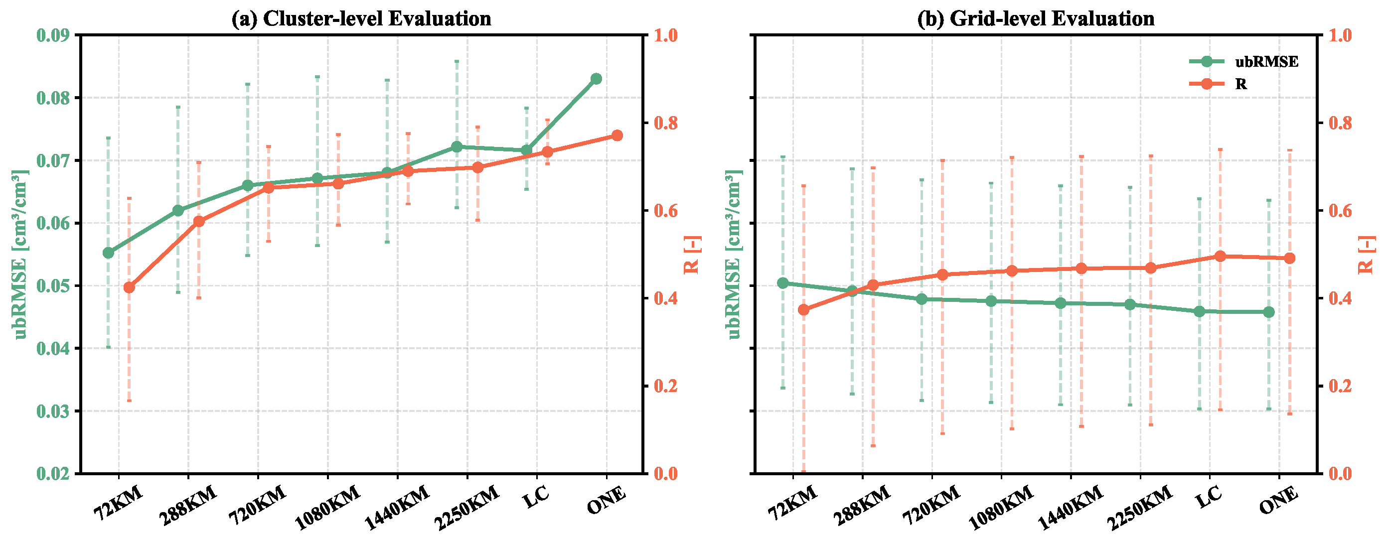
Comparison of ubRMSE () and R between TM-1 and SMAP soil moisture during the testing period under two evaluation schemes: (a) cluster-level and (b) grid-level. The teal curve denotes the ubRMSE metric, and the orange curve denotes the correlation coefficient R; vertical error bars indicate the interquartile range (25–75%), reflecting performance dispersion across cluster or grid scales.
Figure 6.
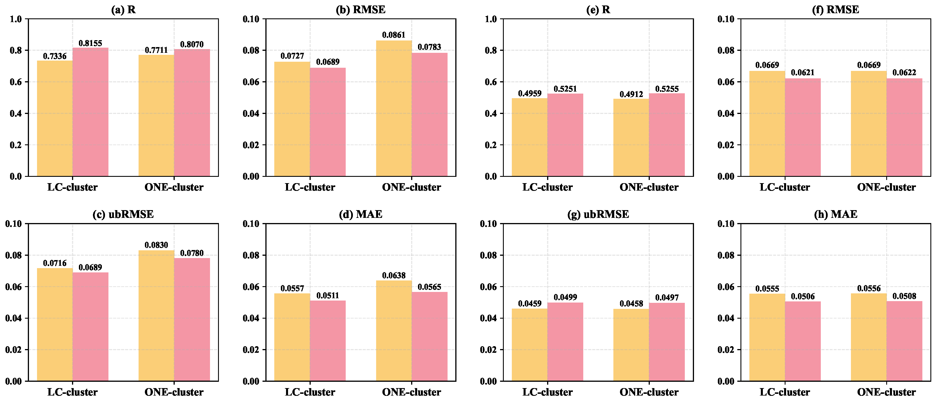
Test results of TM-1 and SMAP soil moisture under different data-splitting schemes. Panels (a–d) show the cluster-level evaluation metrics (R, RMSE, ubRMSE, and MAE) for the LC-cluster and ONE-cluster strategies, while panels (e–h) present the corresponding grid-level evaluation metrics. Yellow and pink bars denote the Time Sequence and Seasonal Sequence splits, respectively.
Figure 7.
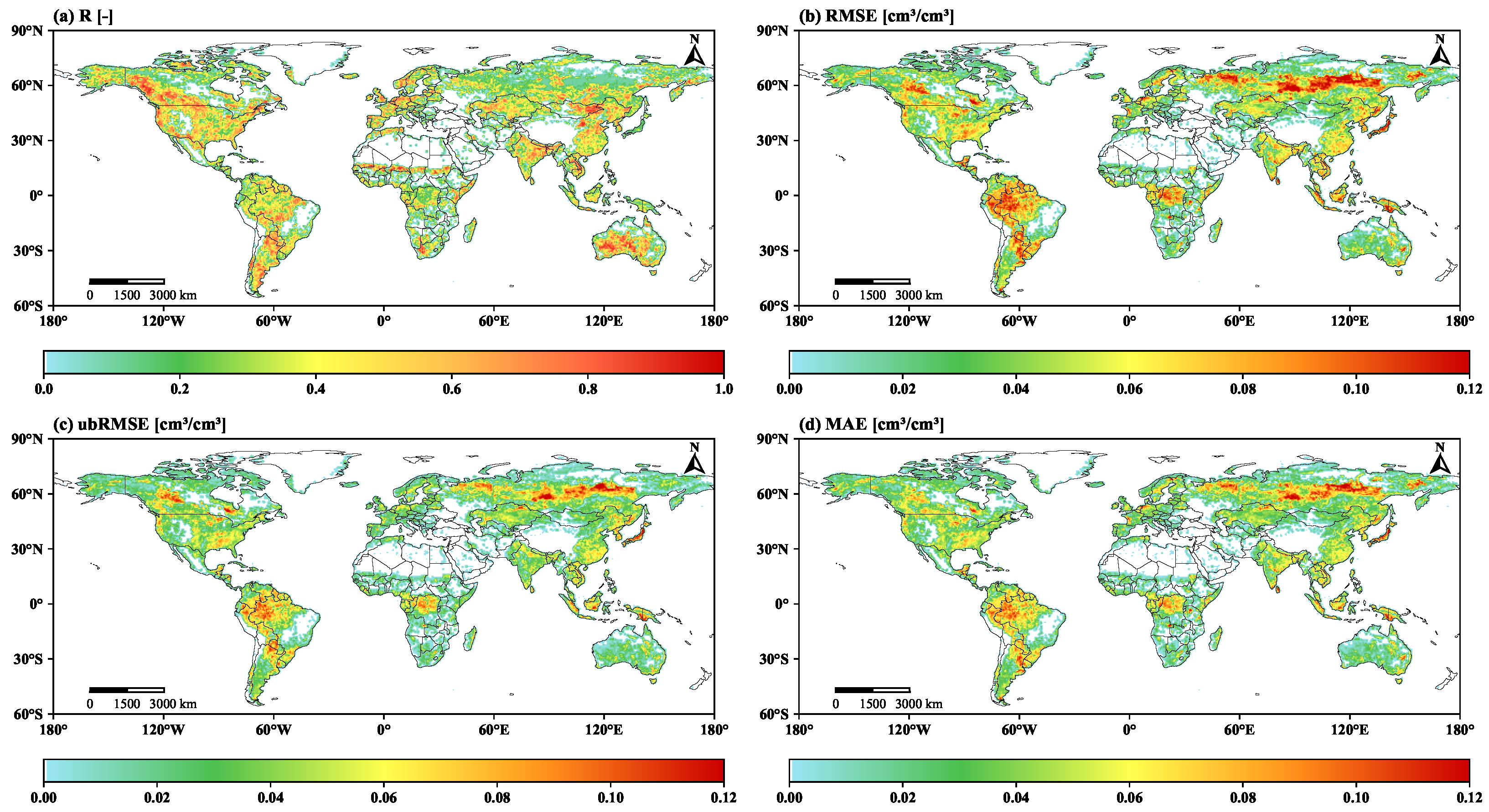
Spatial distribution of test evaluation metrics for TM-1 and SMAP soil moisture under the LC-cluster strategy with seasonal partitioning. Panels (a–d) show R, RMSE (), ubRMSE (), and MAE (), respectively. The color bar beneath each panel indicates the metric values and their corresponding color ranges.
Figure 8.
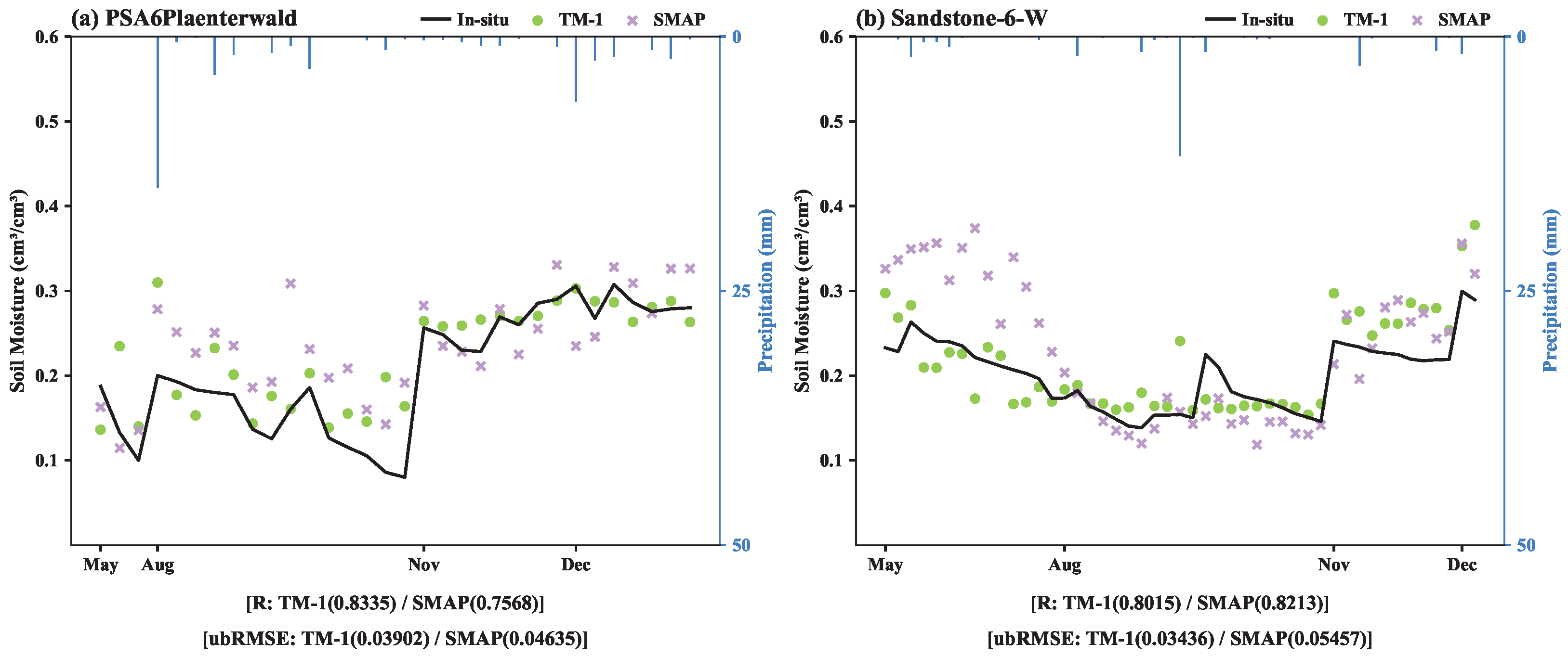
Comparison of TM-1 and SMAP soil moisture predictions against in situ observations at PSA6Plaenterwald and Sandstone-6-W stations (May, August, November, and December 2023). The left y-axis denotes soil moisture, while the right y-axis denotes precipitation.
Figure 8.
Comparison of TM-1 and SMAP soil moisture predictions against in situ observations at PSA6Plaenterwald and Sandstone-6-W stations (May, August, November, and December 2023). The left y-axis denotes soil moisture, while the right y-axis denotes precipitation.
Figure 9.
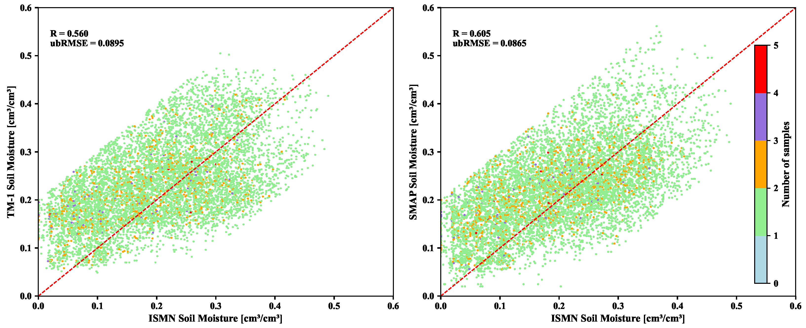
Scatterplots of TM-1 and SMAP soil moisture predictions versus in situ ISMN observations in the test months (May, August, November, December 2023). The red dashed line represents the 1:1 consistency line (). The right-hand color bar maps soil moisture values to their corresponding colors.
Figure 9.
Scatterplots of TM-1 and SMAP soil moisture predictions versus in situ ISMN observations in the test months (May, August, November, December 2023). The red dashed line represents the 1:1 consistency line (). The right-hand color bar maps soil moisture values to their corresponding colors.
Figure 10.
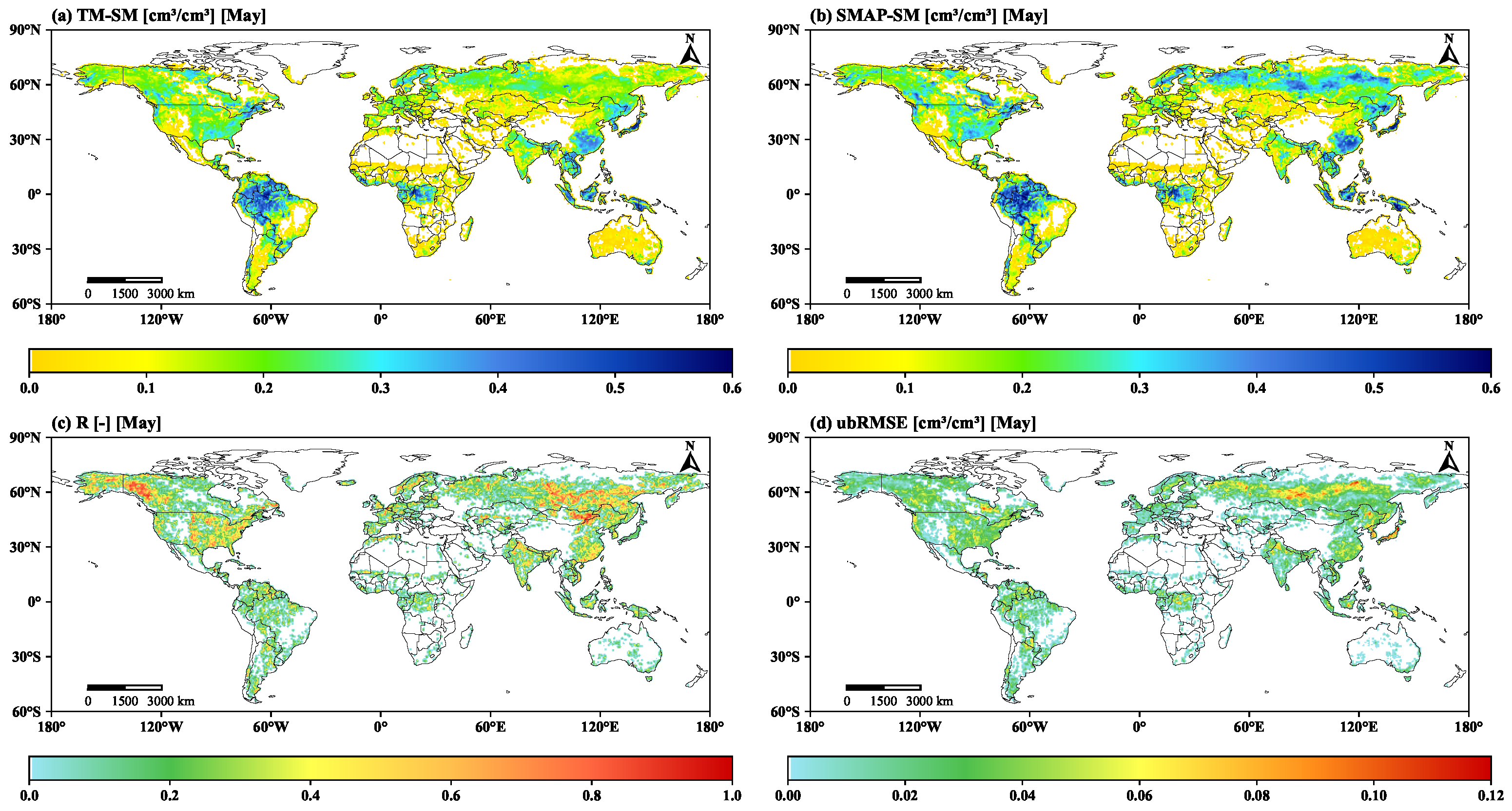
Spatial distribution of TM-1 and SMAP soil moisture and evaluation metrics (ubRMSE (cm3/cm3) and R) for the May test set. The color bar beneath the soil moisture panels indicates the soil moisture values and their corresponding color ranges; the color bars beneath the evaluation-metric panels indicate the respective metric values and their corresponding color ranges.
Figure 11.
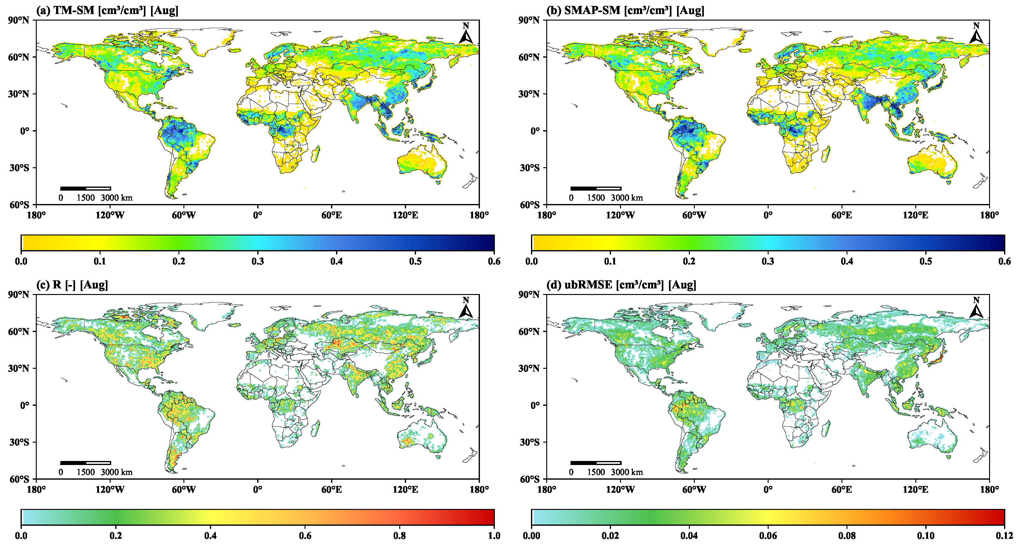
Spatial distribution of TM-1 and SMAP soil moisture and evaluation metrics (ubRMSE (cm3/cm3) and R) for the August test set. The color bar beneath the soil moisture panels indicates the soil moisture values and their corresponding color ranges; the color bars beneath the evaluation-metric panels indicate the respective metric values and their corresponding color ranges.
Figure 12.
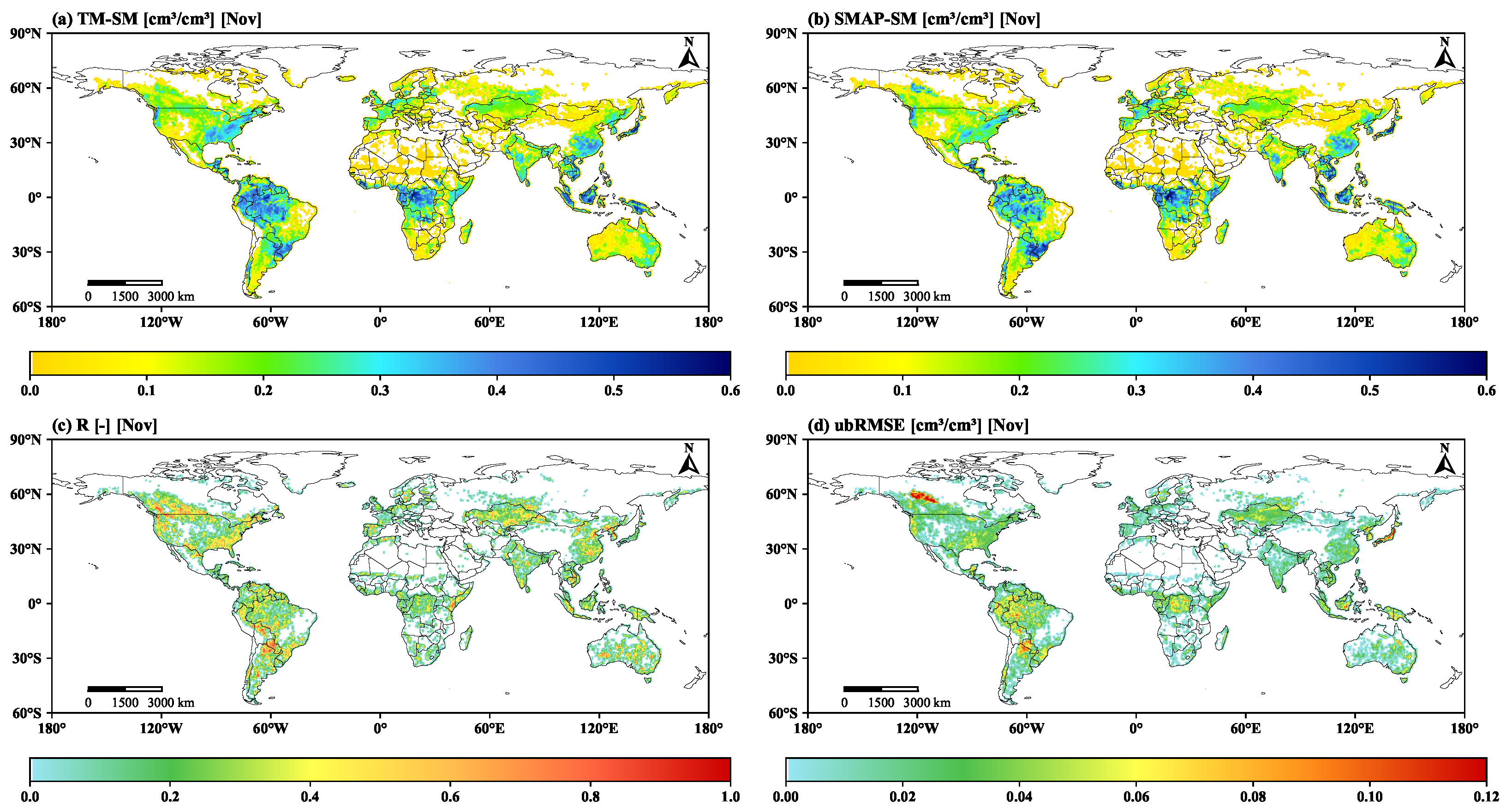
Spatial distribution of TM-1 and SMAP soil moisture and evaluation metrics (ubRMSE (cm3/cm3) and R) for the November test set. The color bar beneath the soil moisture panels indicates the soil moisture values and their corresponding color ranges; the color bars beneath the evaluation-metric panels indicate the respective metric values and their corresponding color ranges.
Figure 13.
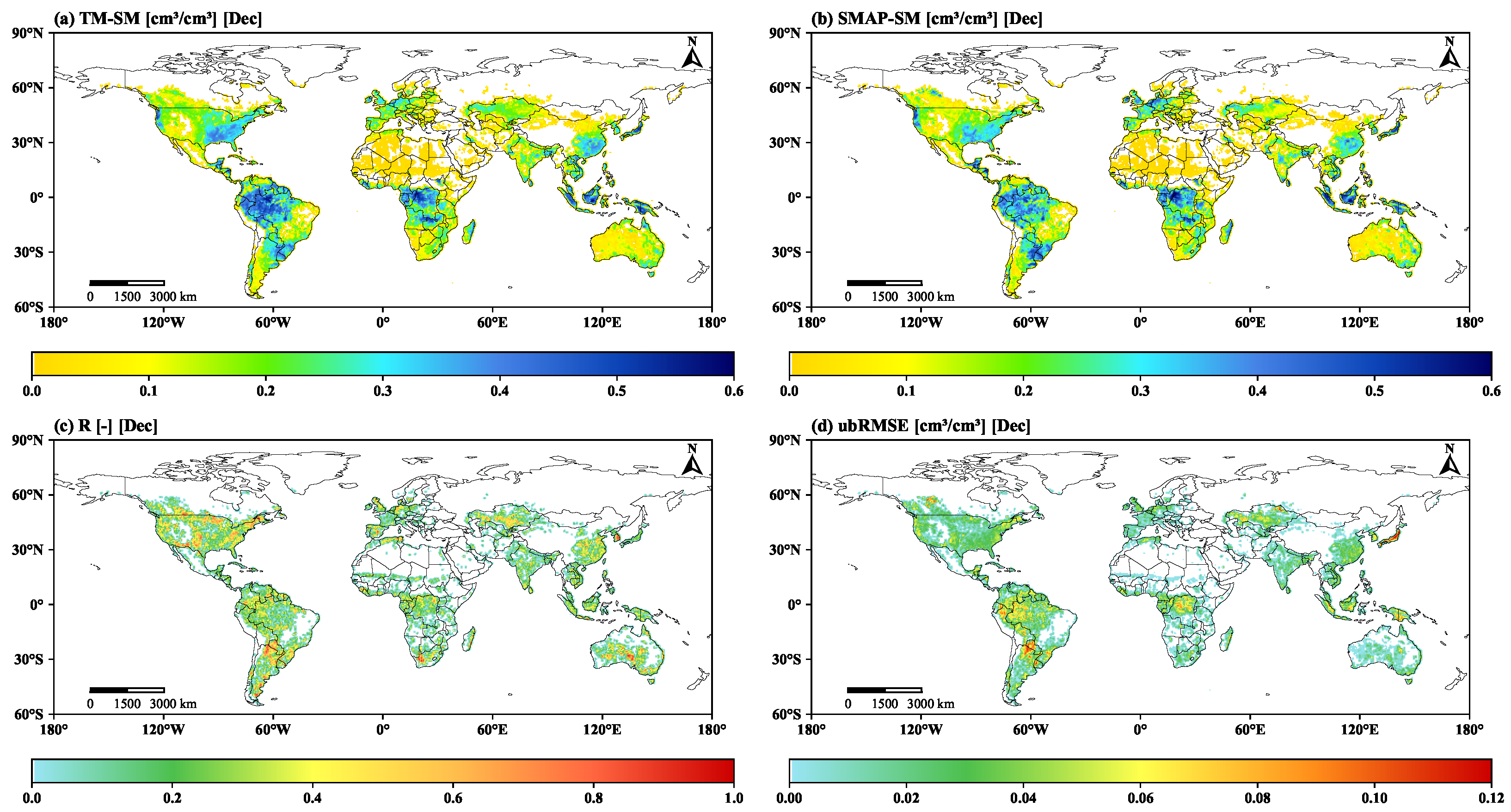
Spatial distribution of TM-1 and SMAP soil moisture and evaluation metrics (ubRMSE (cm3/cm3) and R) for the December test set. The color bar beneath the soil moisture panels indicates the soil moisture values and their corresponding color ranges; the color bars beneath the evaluation-metric panels indicate the respective metric values and their corresponding color ranges.
Figure 14.
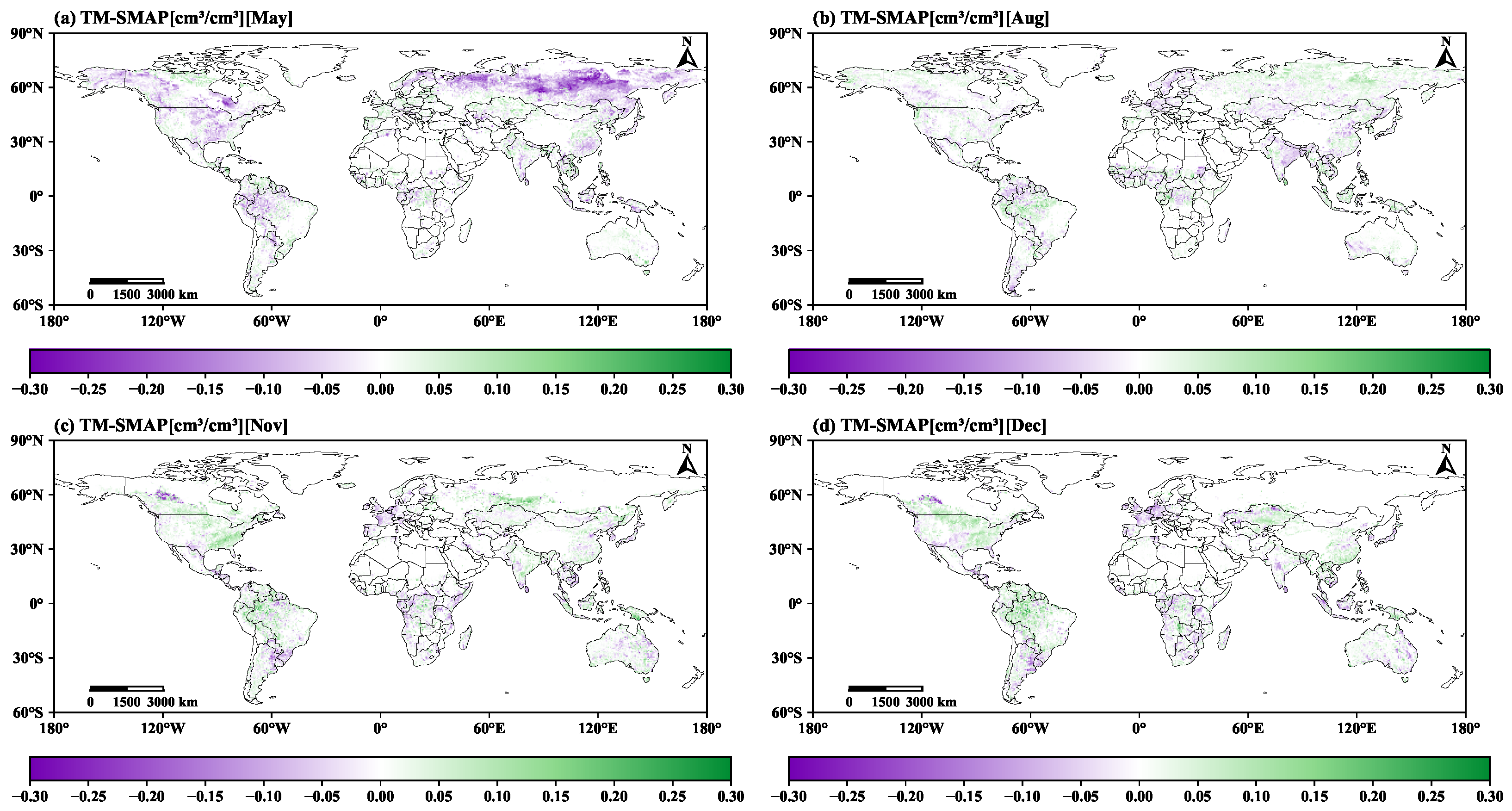
Seasonal mean spatial distribution of the differences (TM-1–SMAP) between TM-1 and SMAP soil moisture retrievals during the 2023 test period (May, August, November, and December). The color bar ranges from −0.30 to 0.30 cm3/cm3; purple indicates that TM-1 is lower than SMAP, while green indicates that TM-1 is higher than SMAP.
Figure 15.
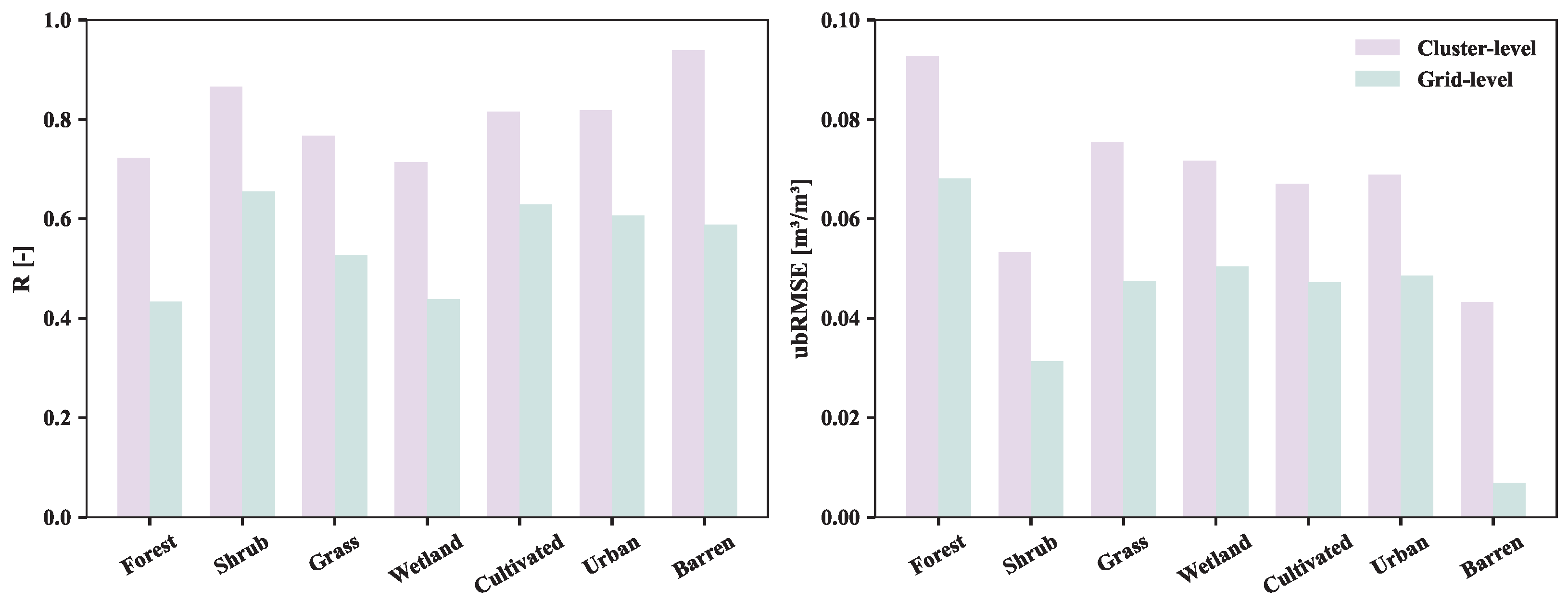
Test-set performance of TM-1 soil moisture retrievals against SMAP under different land-cover types for the LC-cluster plus seasonal-splitting configuration. Purple bars denote cluster-level results (Cluster-level), and green bars denote grid-level results (Grid-level). The metrics shown are the correlation coefficient (R) and the unbiased root-mean-square error (ubRMSE).
Table 1.
Key parameters of TM-1 GNSS-R observations. Units: “–” denotes dimensionless; ° denotes degrees; s denotes seconds; dB denotes decibels. Abbreviations: DDM, Delay–Doppler Map; SNR, signal-to-noise ratio; Rx, receiver.
Table 1.
Key parameters of TM-1 GNSS-R observations. Units: “–” denotes dimensionless; ° denotes degrees; s denotes seconds; dB denotes decibels. Abbreviations: DDM, Delay–Doppler Map; SNR, signal-to-noise ratio; Rx, receiver.
| Name | Units | Description |
|---|
| Ddm_sp_reflectivity | – | Specular point reflectivity |
| Sp_inc_angle | ° | Specular point incidence angle |
| Ddm_kurtosis | – | DDM kurtosis |
| Ddm_skewness | – | DDM skewness |
| Sp_lat | ° | Specular point latitude |
| Sp_lon | ° | Specular point longitude |
| Ddm_time_utc | s | DDM sample time UTC |
| Sp_antenna_gain | dB | Specular point Rx antenna gain |
| Ddm_sp_snr | dB | DDM specular point SNR |
| Ddm_quality_flag | – | DDM quality flag |
| Sp_land_sea_mask | – | Specular point land–sea mask |
Table 2.
Statistics of different clustering strategies for global coverage. 72KM, 288KM, 720KM, 1080KM, 1440KM, and 2250KM clusters represent box-shaped clustering methods with different side lengths at regular intervals. LC-cluster refers to clustering based on land cover types. ONE-cluster represents a single model trained with all global grid cells. The sample count refers to the number of training samples.
| Clustering Strategy | 72KM | 288KM | 720KM | 1080KM | 1440KM | 2250KM | LC | ONE |
|---|
| Number of Models | 26,720 | 2482 | 535 | 277 | 169 | 83 | 7 | 1 |
| Average Samples per Model | 436 | 4640 | 21,540 | 41,615 | | | | |
| Standard Deviation of Samples per Model | 499 | 5648 | 27,029 | | | | | / |
Table 3.
Sample statistics and TM-1/SMAP–ISMN validation metrics for each ISMN network and land-cover type.
Table 3.
Sample statistics and TM-1/SMAP–ISMN validation metrics for each ISMN network and land-cover type.
| Network | Land-Cover Type |
|---|
|
Forest
|
Shrub
|
Grass
|
Cultivated
|
Barren
|
Urban
|
|---|
| Berlin | 228 | – | 20 | 211 | – | 442 |
| CW3E | 102 | – | 323 | 7 | – | 8 |
| FMI | – | – | 49 | – | – | – |
| REMEDHUS | – | 12 | 40 | 100 | – | – |
| RSMN | – | – | – | 17 | – | 2 |
| SCAN | 377 | 85 | 1497 | 874 | 88 | 12 |
| SMOSMANIA | 16 | – | 75 | 52 | – | – |
| SNOTEL | 126 | 136 | 832 | 6 | 15 | 10 |
| SOILSCAPE | – | 98 | 128 | – | – | – |
| USCRN | 303 | 124 | 1191 | 330 | 46 | 41 |
| XMS-CAT | 7 | – | 18 | 51 | – | – |
| n_samples | 1159 | 455 | 4173 | 1648 | 149 | 515 |
| R(TM1–ISMN) | 0.531 | 0.7488 | 0.519 | 0.5375 | 0.7581 | 0.6057 |
| R(SMAP–ISMN) | 0.5814 | 0.7189 | 0.6121 | 0.5618 | 0.7737 | 0.6524 |
| ubRMSE(TM1–ISMN) | 0.0869 | 0.0652 | 0.0919 | 0.0845 | 0.0581 | 0.704 |
| ubRMSE(SMAP–ISMN) | 0.0834 | 0.0685 | 0.0841 | 0.0838 | 0.0572 | 0.0673 |
Table 4.
Feature importance ranking in the TM soil moisture estimation model.
Table 4.
Feature importance ranking in the TM soil moisture estimation model.
| Feature | Importance Mean | Importance Std |
|---|
| VWC | 0.16673 | 0.00079 |
| Precip. | 0.15280 | 0.00058 |
| Rough | 0.12448 | 0.00066 |
| LST | 0.11625 | 0.00065 |
| Clay | 0.10914 | 0.00068 |
| Elev. | 0.05429 | 0.00034 |
| NDVI | 0.01174 | 0.00018 |
Table 5.
Test-set sample statistics and cluster-level performance for each land-cover class.
Table 5.
Test-set sample statistics and cluster-level performance for each land-cover class.
| LC_type | | mean_SMAP | std_SMAP | R | ubRMSE |
|---|
| Forest | 2,025,259 | 0.3577 | 0.1319 | 0.7227 | 0.0926 |
| Shrub | 542,109 | 0.2057 | 0.1037 | 0.8656 | 0.0533 |
| Grass | 3,606,260 | 0.2677 | 0.1168 | 0.7669 | 0.0754 |
| Wetland | 100,491 | 0.2991 | 0.1014 | 0.7140 | 0.0717 |
| Cultivated | 857,491 | 0.2738 | 0.1155 | 0.8155 | 0.0670 |
| Urban | 88,017 | 0.2505 | 0.1198 | 0.8180 | 0.0689 |
| Barren | 216,146 | 0.1222 | 0.1254 | 0.9395 | 0.0433 |
Table 6.
Cluster-level performance comparison of Random Forest and three gradient boosting tree models under the LC-cluster + seasonal partitioning configuration.
Table 6.
Cluster-level performance comparison of Random Forest and three gradient boosting tree models under the LC-cluster + seasonal partitioning configuration.
| Model | R | ubRMSE | RMSE | MAE |
|---|
| CatBoost | 0.7294 | 0.0756 | 0.0772 | 0.0579 |
| LightGBM | 0.7919 | 0.0716 | 0.0733 | 0.0542 |
| XGBoost | 0.7948 | 0.0707 | 0.0726 | 0.0533 |
| Random Forest | 0.8155 | 0.0689 | 0.0689 | 0.0511 |
Table 7.
Grid-level performance comparison of Random Forest and three gradient boosting tree models under the LC-cluster + seasonal partitioning configuration.
Table 7.
Grid-level performance comparison of Random Forest and three gradient boosting tree models under the LC-cluster + seasonal partitioning configuration.
| Model | R | ubRMSE | RMSE | MAE |
|---|
| CatBoost | 0.4820 | 0.0502 | 0.0692 | 0.0578 |
| LightGBM | 0.5033 | 0.0498 | 0.0662 | 0.0548 |
| XGBoost | 0.5202 | 0.0493 | 0.0648 | 0.0535 |
| Random Forest | 0.5251 | 0.0499 | 0.0621 | 0.0506 |
