Spatio-Temporal Dynamics and Driving Mechanism of Ecosystem Services Under Ecological Restoration in the Kubuqi Desert, Northern China

Abstract

Desertification is an ever-growing global ecological and environmental problem. With the implementation of various ecological restoration initiatives, vegetation cover in many desert regions has increased substantially. Consequently, it is essential to understand the dynamics of ecosystem services (ESs) in desert ecosystems to better inform environmental management. This study integrates the InVEST model, RWEQ model, Spearman correlation analysis, trade-off and synergy coefficient method, and the Partial Least Squares Path Model (PLS-PM) to systematically assess the spatio-temporal dynamics and underlying driving mechanisms of five key ESs in the Kubuqi (KBQ) Desert, northern China. Specifically, the application of PLS-PM enables the identification of latent pathways, indirect effects, and multi-step causal relationships, which traditional correlation-based methods fail to capture. The results show that the KBQ Desert underwent substantial land use changes from 2000 to 2020: sandy land decreased by 2697.83 km², grassland increased by 1864.15 km², and cropland and urban land expanded by 519.15 km² and 257.74 km², respectively. ESs exhibited divergent trajectories. habitat quality (HQ), carbon sequestration (CS), soil conservation (SC), and water yield (WY) all showed overall increases, with WY and SC increasing particularly strongly, whereas Sand-fixation service (G) displayed a fluctuating trend. Over the past two decades, HQ–CS, HQ–G, and CS–G have shown moderately strong synergies, while CS–WY has exhibited a pronounced trade-off, and SC–G and SC–CS have displayed relatively weaker trade-offs. The spatial distribution results of trade-off and synergy relationships show that the KBQ Desert is dominated by a synergy relationship, and the main synergy relationship combinations are CS–HQ, CS–SC, and HQ–SC. The correlation coefficients between other ES pairs are generally low. Additionally, this study identifies key pathways through the PLS-PM method, such as PRE → NDVI → ES and LU → NDVI → ES, revealing the complex interactions between precipitation (PRE), land use (LU), and vegetation dynamics. The findings show that land use (LU) consistently exerts a strong negative impact on CS, while PRE and NDVI have a significant positive effect on WY. These pathways deepen our understanding of how climate and anthropogenic factors affect ESs, particularly the influence of temperature (TEMP) on evapotranspiration (ETP), which in turn affects WY. Additionally, the impact of NDVI on wind–sand fixation (G) and SC varies over time, with vegetation dynamics playing a particularly enhanced role in 2010 and 2015. These findings highlight the impact of ecological restoration and land management on regional ESs changes. A comprehensive understanding of the interactions between climate factors, LU, and vegetation dynamics will help in developing more effective intervention strategies.

1. Introduction

Covering over 40% of the Earth’s land surface, desert ecosystems are among the most fragile and sensitive to land cover change due to their extreme climatic conditions and sparse vegetation [1,2]. Their limited resilience makes them highly vulnerable to degradation, whereby even minor disturbances can result in persistent ecological decline [3,4,5]. Therefore, ecological restoration work in desertified areas require more refined scientific evidence as support, and understanding the changing characteristics of regional ecosystem services (ESs) is crucial for guiding the effective management and sustainable development strategies of arid areas.

Ecosystem service (ES) plays a vital role in connecting humanity with the natural world, being essential to human production, livelihoods, and overall well-being [6]. Changes in land structure are a significant cause of shifts in regional Ess [7]. On one hand, the intensification of human activities leads to rapid changes in land structure and nature, thereby affecting the provision of Ess [8]. On the other hand, different land management and usage practices can cause fluctuations in the stability of ES outputs. Consequently, most studies analyze the characteristics of land-use change to reveal the alterations in ESs [7]. In response to widespread land degradation, large-scale ecological restoration projects such as the Mediterranean coastal lagoon restoration, the Altyn Dala Conservation Initiative in Central Asia, and China’s Three-North Shelterbelt Program have played a pivotal role in improving ecological stability and restoring key ecosystem functions in arid landscapes [9,10,11]. These efforts have significantly contributed to the stabilization and restoration of ecosystem structure and function at regional and global scales. Recent studies in arid regions, particularly in Central Asia and northern China, have focused on understanding the dynamics of ESs. Findings consistently highlight that climate variability and land-use change are the dominant drivers of ES dynamics, while large-scale ecological interventions have contributed significantly to service enhancement. For example, long-term vegetation restoration and water soil conservation projects in northern China have led to substantial improvements in regulating services such as wind erosion control and carbon storage [12,13]. In Central Asia, ESs exhibit pronounced spatial heterogeneity driven by both natural gradients and anthropogenic pressures. Methodologically, recent advancements such as ES network (ESN) analysis, wind erosion modeling (e.g., RWEQ), and spatially explicit assessments have improved our understanding of ES interactions and temporal evolution [14]. Research on desert ESs, particularly regarding their dynamic changes and underlying mechanisms, remains insufficient. Many studies are typically conducted at broad spatial scales, often overlooking localized patterns that are crucial for site-specific management [15]. Given the high spatial heterogeneity of desert ecosystems, fine scale assessments are essential to identify localized trade-offs and synergies, thereby providing more targeted support for ecological restoration efforts. While considerable attention has been given to specific ESs such as SC and CS, the complex interactions between natural factors and anthropogenic influences have not been sufficiently explored. These interactions, including nonlinear relationships among multiple drivers, require further investigation to provide effective solutions for ecological restoration in desertified regions. In conclusion, our understanding of the dynamic characteristics of ESs at fine scales, and how different influencing factors affect changes in ESs, remains limited, hindering the development of effective management strategies for sustainable ecological restoration in desert regions.

Furthermore, many studies have investigated the factors influencing regional changes in ESs using methods such as correlation analysis and geographical detectors, with the aim of identifying the primary and secondary drivers of these changes [16,17]. While these studies have provided insights into the causes of ES changes, the complex and nonlinear driving mechanisms underlying these changes remain inadequately understood. The interactions between influencing factors and the specific impact pathways of ESs are intricate and multifaceted. In particular, the driving processes of desert ecosystems service are characterized by high complexity, nonlinearity, and multi-factorial interactions [18]. The dynamics of desert ecosystems are shaped by a variety of interacting natural and anthropogenic factors, making it difficult for traditional methods to fully capture the complexity of these driving processes. In this context, the application of Partial Least Squares Path Modeling (PLS-PM) represents a significant breakthrough, effectively overcoming the limitations of traditional analytical methods. PLS-PM enables the exploration of these complex dynamics, revealing latent pathways, indirect effects, and multi-step causal chains that traditional methods often overlook. Unlike traditional correlation-based approaches, PLS-PM can handle highly complex and multidimensional data, making it particularly well-suited for studying ecosystems where multiple factors interact in a nonlinear and dynamic manner. Additionally, PLS-PM allows for the analysis of both direct and indirect relationships between variables, providing a more holistic view of the drivers influencing ESs. By applying PLS-PM to the dynamics of ESs in the Kubuqi (KBQ) Desert, this study addresses the need for a more nuanced understanding of how various drivers interact to influence ESs in desert ecosystems, offering insights that are essential for in-formed environmental management and restoration strategies.

The KBQ Desert, located to the north of Ordos City in Inner Mongolia, China, is a major source of wind and sand for the Beijing–Tianjin–Hebei region. It holds significant scientific relevance in terms of regional ecological environmental changes and ecological restoration efforts. The desert ecosystem in this region has undergone substantial transformations due to climate change, land use alterations, and the implementation of ecological restoration projects. Understanding the complex interactions among these factors is crucial for improving ecological management strategies and mitigating desertification. Furthermore, the unique ecological characteristics of the KBQ Desert, such as its vulnerability to sandstorms and the impact of large-scale human interventions, make it an invaluable model for studying desert ESs and their resilience. To address these scientific questions, this study employs an integrated methodological framework that combines InVEST, RWEQ, and PLS-PM. The InVEST model provides a comprehensive assessment of ES values, which is essential for understanding the spatial distribution of these services in the KBQ Desert. The RWEQ model is used to simulate wind erosion and its effects on desertification and ESs, particularly SC and WY. PLS-PM, as a multivariate statistical tool, is capable of exploring nonlinear interactions between multiple driving factors, such as land use, climate variables, and human interventions, identifying the most significant pathways and indirect effects. Our research aims to comprehensively evaluate the spatio-temporal dynamics of ESs in the KBQ Desert from 2000 to 2020, with a focus on quantifying service changes, exploring their interactions, and identifying driving mechanisms. The specific objectives are to: (1) analyze land use changes over the past two decades; (2) quantify the spatial and temporal variations of five representative ESs (HQ—Habitat Quality, CS—Carbon Sequestration, SC—Soil conservation, WY—Water Yield, G—Sand-fixation service); (3) investigate trade-offs and synergies among these services; and (4) investigate and analyze the driving mechanisms behind changes in various services. The findings of this study are expected to provide valuable insights into the ecosystem changes in desert environments and offer scientific support for precision ecological management and policy formulation in arid and semi-arid regions.

2. Materials and Methods

2.1. Study Area

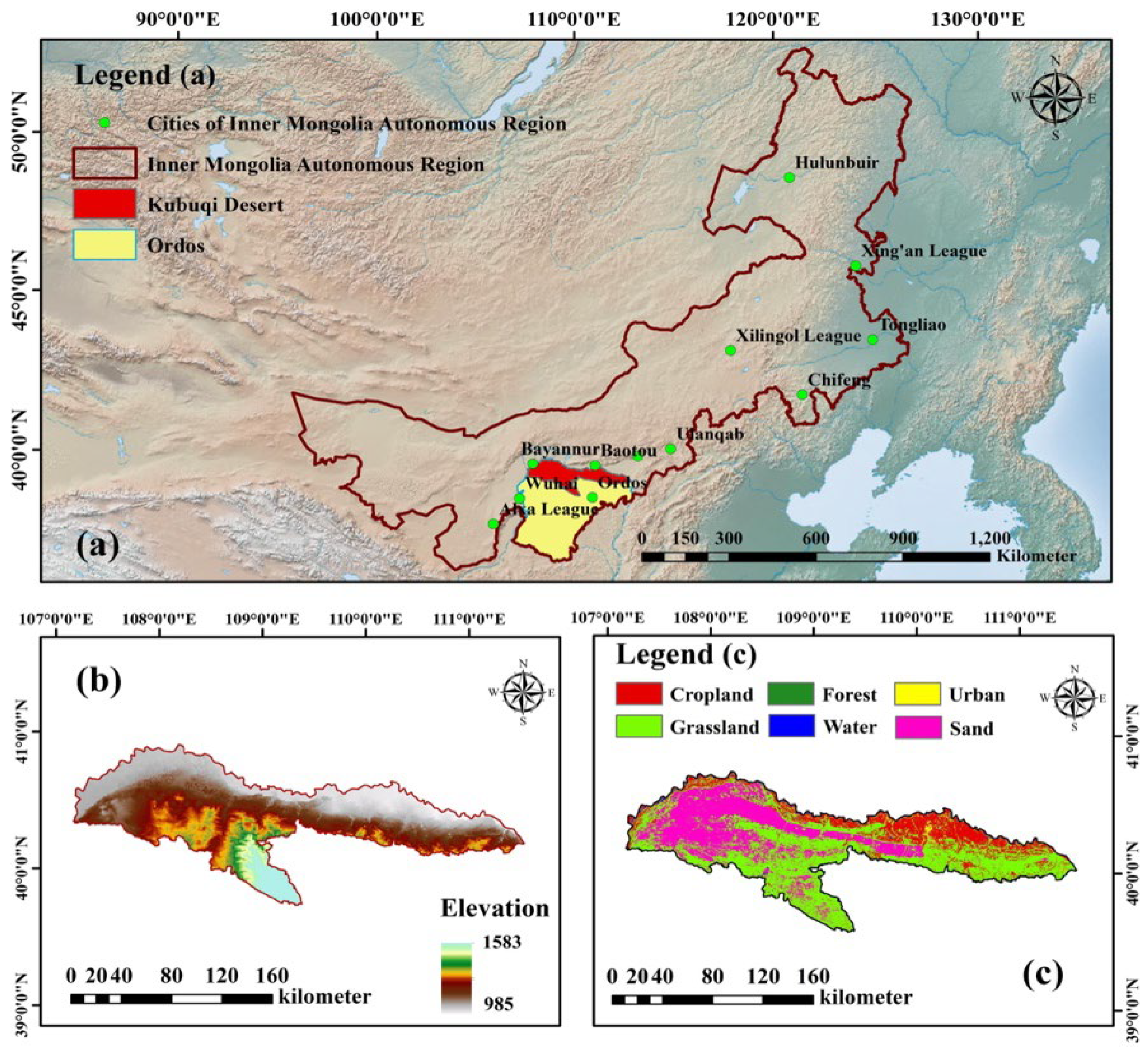
The KBQ Desert is in the middle reaches of the Yellow River, within the northern part of the Ordos Plateau, Inner Mongolia Autonomous Region, China. It extends longitudinally from west to east, approximately between 107.0–111.3° E and 39.15–40.45° N, occupying the northern part of the Ordos Plateau in Inner Mongolia (Figure 1). Situated in a typical temperate continental arid to-semi-arid monsoon climate zone, the region experiences significant temperature variability, with a mean annual temperature of approximately 11.2 °C. Annual precipitation ranges from 100 to 280 mm, while annual potential evapotranspiration exceeds 2000 mm during the study period, indicating a severe moisture deficit. These features collectively highlight the harsh natural environmental conditions faced by the region. Although a series of large-scale ecological restoration programs have substantially improved the overall ecological status of the KBQ Desert in recent decades, localized areas still suffer from low environmental quality and high vulnerability. Furthermore, uneven regional development and spatially unbalanced ecological recovery have emerged as key challenges for sustainable environmental governance in the area. Against this backdrop, a detailed understanding of the spatio-temporal dynamics of ESs in the KBQ Desert is essential for informing future ecological planning and optimizing restoration strategies.

2.2. Data Resource

To ensure the accuracy and consistency of ES assessments, this study integrated a comprehensive set of geospatial and environmental datasets. Details on data sources and specifications are provided in

Table 1. Data utilized in research.

Data	Spatial Resolution	Resource
Land use	30 m	Yang, J., & Huang, X. (2021). China Land Cover Dataset (CLCD). Wuhan University. Retrieved from https://zenodo.org/records/12779975 [19]
Evapotranspiration	1 km	Peng, S., Ding, Y., Wen, Z., Chen, Y., Cao, Y., & Ren, J. (2023). 1 km Monthly Potential Evapotranspiration Dataset for China (1901–2022). National Tibetan Plateau/Third Pole Environment Data Center. Retrieved from https://data.tpdc.ac.cn/en/data/8b11da09-1a40-4014-bd3d-2b86e6dccad4 [20]
Population density	1 km	Sims, K., Reith, A., Bright, E., Kaufman, J., Pyle, J., Epting, J., Gonzales, J., Adams, D., Powell, E., Urban, M., & Rose, A. (2023). LandScan Global 2022 [Data set]. Oak Ridge National Laboratory. https://doi.org/10.48690/1529167 [21]
DEM	1 km	U.S. Geological Survey (USGS). Digital Elevation Model (DEM) Data from EarthExplorer [Data set]. U.S. Department of the Interior. Available from USGS EarthExplorer: https://earthexplorer.usgs.gov/
NDVI	1 km	National Earth System Science Data Center. Normalized Difference Vegetation Index (NDVI) Dataset [Data set]. China. Available from https://www.geodata.cn/
Snow depth	1 km	National Earth System Science Data Center & RESDC. Snow depth dataset (1 km resolution). National Earth System Science Data Center, China. Retrieved from http://www.resdc.cn/
Soil dataset	N/A	Food and Agriculture Organization of the United Nations (FAO), International Institute for Applied Systems Analysis (IIASA), & Others. (2012). Harmonized World Soil Database (Version 1.2) [Soil dataset]. FAO & IIASA. Retrieved from https://www.fao.org/soils-portal/soil-survey/soil-maps-and-databases/harmonized-world-soil-database-v12/en/ [22]
Precipitation, wind speed, temperature	N/A	China Meteorological Data Service Center. Meteorological observation data for China: precipitation, temperature, and wind speed [Dataset]. China Meteorological Data Service Center (CMDC). Retrieved from https://data.cma.cn/ [23]

. Land use data were derived from the 30 m-resolution China Land Cover Dataset (CLCD), produced by Wuhan University (https://zenodo.org/records/12779975, accessed on 15 January 2025). Evapotranspiration data (1 km-resolution) was obtained from the Loess Plateau Science Data Center. Daily meteorological variables, including PRE, WS, and TEMP, were sourced from the National Ground Meteorological Station Dataset (V3.0), published by the China Meteorological Administration (https://data.cma.cn/, accessed on 5 February 2025). Population density estimates were extracted from the 1 km-resolution LandScan Global Population Database (https://landscan.ornl.gov, accessed on 10 March 2025). Normalized Difference Vegetation Index (NDVI) data with 1 km × 1 km grid were acquired from the National Earth System Science Data Center (https://www.geodata.cn, accessed on 20 April 2025), while snow depth data (1 km-resolution) were obtained from the Resource and Environment Science and Data Center, Chinese Academy of Sciences (http://www.resdc.cn, accessed on 1 May 2025). Soil property data were retrieved from the Harmonized World Soil Database (HWSD) provided by the FAO (https://www.fao.org/soils-portal/soil-survey/soil-maps-and-databases/harmonized-world-soil-database-v12/en/, accessed on 15 June 2025). To maintain analytical consistency, all datasets were resampled to a unified spatial resolution of 1 km using nearest-neighbor interpolation in ArcGIS 10.8.

2.3. Research Method

The five ESs in the KBQ Desert were quantified by integrating the InVEST model (for CS, SC, WY and HQ) with the RWEQ model (for G).

2.3.1. Habitat Quality

The module evaluates habitat quality from two perspectives: the intensity of external threats and the intrinsic sensitivity of the threatened ecosystem. Generally, areas with high Habitat quality correspond to stable natural ecosystems subject to few stressors. The habitat quality index (HQI) quantitatively reflects habitat conditions [17]. The calculation formula is as follows:

$$Q_{xj}=H_j\times \left[1-\left({\displaystyle \frac{D_{xj}^z}{D_{xj}^z+k^z}}\right)\right]$$

(1)

where Q_xj and D_xj denote the HQ and threat level, respectively, for land-use type j in grid cell x; H_j is the habitat suitability of land-use type j; z (commonly set to 2.5) is the normalization constant; and k is the half-saturation constant.

2.3.2. Soil Conservation

We employed the InVEST sediment-delivery ratio (SDR) module to assess soil-retention services. Building on the Universal Soil Loss Equation (USLE), the module incorporates upslope sediment retention at the raster level to enhance computational accuracy [24]. Potential soil erosion and actual soil erosion were derived for each grid cell, and the soil-retention volume (SR) was calculated as the difference between the two:

$$SR=RKSE-USLE$$

(2)

$$RKLE=R\times K\times LS$$

(3)

$$USLE=R\times K\times LS\times C$$

(4)

where SR denotes the soil conservation amount, RKLS and USLE represent potential and actual soil erosion, respectively, and R, K, LS, C, and P are the rainfall erosivity, soil erodibility, slope length and steepness, vegetation cover management, and conservation-practice factors.

2.3.3. Water Yield

Water yield service was calculated using the Water yield module in the InVEST model, which is based on the water balance principle and Budyko’s coupled water-heat balance assumption; Water yield was computed as the difference between precipitation and actual evapotranspiration to represent Water yield in the study area [25]. The specific calculation formula is as follows:

$$Y_{xj}=\left(1-{\displaystyle \frac{{AET}_{xj}}{P_x}}\right)\times P_x$$

(5)

where Y_xj is the annual WY (mm) for land use type j in grid cell x; P_x is the mean annual precipitation (mm) for grid cell x; and AET_xj is the actual annual evapotranspiration (mm) for land-use type j in grid cell x.

2.3.4. Carbon Sequestration

Carbon Sequestration reflects the terrestrial ecosystem’s capacity for Carbon storage In this study, the InVEST carbon storage module was employed to quantify regional carbon stocks, incorporating four distinct carbon pools: above-ground biomass, below-ground biomass, soil organic carbon, and dead organic matter [26]. The total carbon stock (C_total) is calculated as:

$$C_{total}=C_{above}+C_{blow}+C_{soil}+C_{dead}$$

(6)

where C_total is the total carbon stock, and C_above, C_below, C_soil and C_dead denote the carbon stored in above-ground biomass, below-ground biomass, soil, and dead organic matter, respectively.

2.3.5. Sand-Fixation Service

Owing to its high accuracy and applicability for quantifying wind-erosion regulation services, the Revised Wind Erosion Equation Model (RWEQ) has been widely applied in desertified regions. The RWEQ model is primarily designed with five key factors: WF (Wind Force), EF (Erosion Factor), SCF (Soil Crust Factor), K′ (Topographic Roughness Factor), and C (Vegetation Factor). WF represents the effect of wind speed on soil erosion, where higher wind speeds exacerbate erosion, while lower wind speeds reduce it. EF describes the erodibility of the soil, with looser or more fragile soils being more susceptible to wind erosion. SCF indicates the impact of the soil surface crust in resisting wind erosion, where a crust layer can reduce wind speed and mitigate erosion, although a thick crust can affect soil permeability and water infiltration. K′ reflects the roughness of the terrain, where variations in topography affect wind flow patterns and influence wind erosion, with rougher terrain generally reducing erosion intensity. Lastly, C represents the protective effect of vegetation cover, which helps anchor the soil, reducing direct wind impact and thereby slowing down erosion. Together, these factors interact to determine the extent and rate of soil erosion in the study area, providing a comprehensive framework for understanding and managing wind erosion. In this study, the RWEQ model was employed to compute the potential wind erosion, actual wind erosion, and G capacity within the study area from 2000 to 2020, thereby enabling an assessment of soil wind-erosion dynamics. All parameters were calibrated according to both model specifications and local conditions [27]. The governing equation is as follows:

$$Q_{\mathit{max}1}=109.8\times \left[WF\times EF\times SCF\times K^{\prime }\right]$$

(7)

$$S_1=150.71\times {\left[WF\times EF\times SCF\times K^{\prime }\right]}^{-0.3711}$$

(8)

$$S_{L_1}={\displaystyle \frac{2Z}{S_1^2}}{Q}_{max1}\times e^{{-\left({\displaystyle \frac{z}{S_1}}\right)}^2}$$

(9)

$$Q_{max}=109\times \left[WF\times EF\times SCF\times K^{\prime }\times C\right]$$

(10)

$$S=150.71\times {\left[WF\times EF\times SCF\times K^{\prime }\times C\right]}^{-0.3711}$$

(11)

$$S_L={\displaystyle \frac{2z}{S^2}}{Q}_{max}\times e^{-{\left({\displaystyle \frac{z}{s}}\right)}^2}$$

(12)

$$G=S_{L_1}-S_L$$

(13)

where G is the sand-fixation amount, $S_{L_1}$ is the potential wind erosion, S_L is the actual soil erosion, S₁ is the potential regional erosion coefficient, S is the regional sand-fixation coefficient, Q_max1 is the potential maximum wind-erosion transport, Q_max is the sand-trapping amount, Z is the distance to maximum wind erosion, WF is the climatic factor, EF is the soil erodibility factor, SCF is the soil crust factor, K′ is the topographic roughness factor, and C is the vegetation factor.

2.3.6. Cold and Hot Spot Analysis

Through the cold and hot spot analysis method, the distribution patterns of different ESs across various periods are clarified. The cold and hot spot analysis (Getis–Ord G_i* statistic) is used to identify spatial hot spots (clusters of high values) and cold spots (clusters of low values). By calculating the G_i* statistic for each feature, it determines whether the clustering of high or low values around it is significant, thereby effectively revealing the spatial agglomeration characteristics of geographical phenomena [16,28]. The specific formula is as follows:

$$G_i^{*}={\displaystyle \frac{{\sum }_{j=1}^n{w}_{i,j}{x}_j-X{\sum }_{j=1}^n{w}_{i,j}}{S\sqrt{\frac{\left[n{\sum }_{j=1}^n{w}_{i,j}^2-{\left({\sum }_{j=1}^n{w}_{i,j}\right)}^2\right]}{n-1}}}}$$

(14)

$$S=\sqrt{{\displaystyle \frac{{\sum }_{j=1}^n{x}_j^2}{n}}-{\left(\overline{X}\right)}^2}$$

(15)

$$\overline{X}={\displaystyle \frac{{\sum }_{j=1}^n{x}_j}{n}}$$

(16)

where G_i^* is the Getis–Ord statistic at location i; w_ij is the spatial weight, representing the spatial adjacency relationship between location i and j; x_j is the value of ESs and other elements at location j; n is the total number of spatial units in the study area; $\overline{X}$ is the average value of element values in all spatial units; S is the standard deviation of element values in all spatial units.

2.3.7. ES Trade-Off and Synergy Analysis

Spearman correlation analysis is a non-parametric statistical method for measuring the strength and direction of association between two variables without assuming a specific distribution. It is particularly robust for non-normal data and effective for ordinal or ranked variables. The computation is straightforward and readily implemented when data is already in rank form. In this study, after performing range-based normalization to render the data dimensionless, Spearman correlation analysis was applied to identify trade-offs and synergies among the different Ess [29]. The specific calculation formula is as follows:

$$Rxy={\displaystyle \frac{{\sum }_{n=1}^n\left(X_{ij}-\overline{X}\right)\left(Y_{ij}-\overline{Y}\right)}{\sqrt{{\sum }_{n=1}^n{\left(X_{ij}-\overline{X}\right)}^2}\sqrt{{\sum }_{n=1}^n{\left(Y_{ij}-\overline{Y}\right)}^2}}}$$

(17)

where R_xy is the correlation coefficient ranging from −1 to 1; a positive value (R_xy > 0) indicates synergy between two ESs, whereas a negative value (R_xy < 0) denotes a trade-off. X_ij and Y_ij represent the values of different ES types.

To further clarify the spatial trade-offs and synergies between different ESs, this study employs a combination of tradeoff-synergy criteria (TSC) and tradeoff-synergy index (TSI) to analyze the relationships between various types of services across different spatial locations [30].

$$TSC={\displaystyle \frac{{ESC}_{{i,t}_2}-{ESC}_{{i,t}_1}}{{ESC}_{{j,t}_2}-{ESC}_{{j,t}_1}}}$$

(18)

$$TSI=1-\left|\left|{∆ES}_i\right|-\left|{∆ES}_j\right|\right|$$

(19)

${ESC}_{{i,t}_2}$ and ${ESC}_{{i,t}_1}$ denote the ES value of type i in the t₂ and t₁ periods, respectively. Similarly, ${ESC}_{{j,t}_2}$ and ${ESC}_{{j,t}_1}$ represent the ES value of type j in the t₂ and t₁ periods, respectively. When the result of $TSC$ is greater than 0, it indicates that the changes of the two ES types are in the same direction, and thus, the pair ES_i and ES_j is recognized as having a synergistic relationship; otherwise, there exists a trade-off relationship between them. Where ES_i and ES_j are the differences in ES values between two periods for types i and j, respectively. The TSI is the tradeoff-synergy index, ranging from 0 to 1. A higher value of this index indicates a stronger intensity of either trade-off or synergy between the ESs.

2.3.8. Analysis of ES Driving Mechanisms

Uncertainty exists in the factors contributing to changes in desert ESs; accordingly, defining the driving mechanisms behind such changes is of critical guiding significance for understanding regional ESs. In this study, the Partial Least Squares Path Modeling (PLS-PM) was applied to investigate the driving mechanisms underlying various types of ESs in the KBQ Desert. The objectives were to uncover how the driving mechanisms of each service changed over different periods and to quantify the magnitude of the effects exerted by various influencing factors on each service. Unlike traditional covariance-based structural equation modeling (CB-SEM), this model does not require measured variables to conform to a normal distribution and imposes less strict demands on sample size, which are two key advantages for ecological data analysis [31]. It uncovers the associations between observed variables and latent variables by combining principal component analysis, multiple regression, and iterative estimation techniques [32]. Consequently, this model can effectively uncover the driving mechanisms behind changes in regional ESs. All statistical analyses, model estimation, bootstrapping, and validation were conducted within the R statistical computing environment (version 4.3.1; R Core Team, 2023, Vienna, Austria). Specifically, the Partial Least Squares Path Modeling was performed using the plspm package (version 0.5.0). This research selected nine influencing factors relevant to the KBQ Desert to analyze the driving mechanisms of ESs. These factors include temperature (TEMP), precipitation (PRE), land use (LU), population density (POP), evapotranspiration (ETP), wind speed (WS), vegetation (NDVI), and topographic factors (DEM and SLOPE).

3. Results

3.1. LU Change of the KBQ Desert

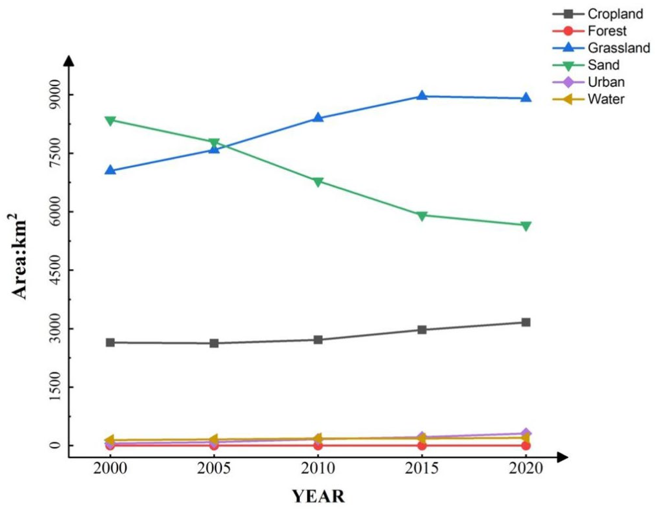
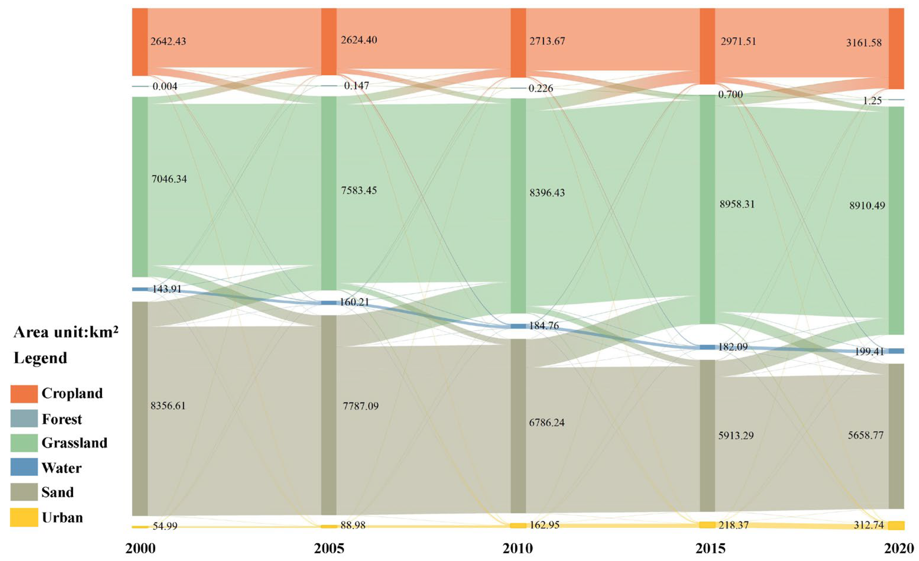
We synthesize the land-use change trajectories of the KBQ desert across five time periods from 2000 to 2020 (Figure 2). Throughout these periods, cropland, sand, and grassland consistently accounted for more than 95% of the total area excluding sand; all other LU types showed net gains between 2000 and 2020. Grassland expanded significantly from 7046 km² in 2000 to 8910 km² in 2020, representing a net increase of 1864 km². Urban land experienced a dramatic growth of 468.7%, highlighting a strong trend of urbanization in the region. Cropland increased by 519 km², marking the second-largest absolute gain after grassland. The Sankey diagram of LU transitions shows a significant reduction in shifting sands, with most being converted into grassland, and a lesser amount into cropland (Figure 3). Across all periods, there was also a consistent flow of land conversion from grassland to cropland. These findings indicate that the KBQ Desert underwent substantial LU transformations between 2000 and 2020. Such rapid land-cover changes are likely to have significant impacts on the region’s ESs.

3.2. Spatio-Temporal Dynamics of ESs

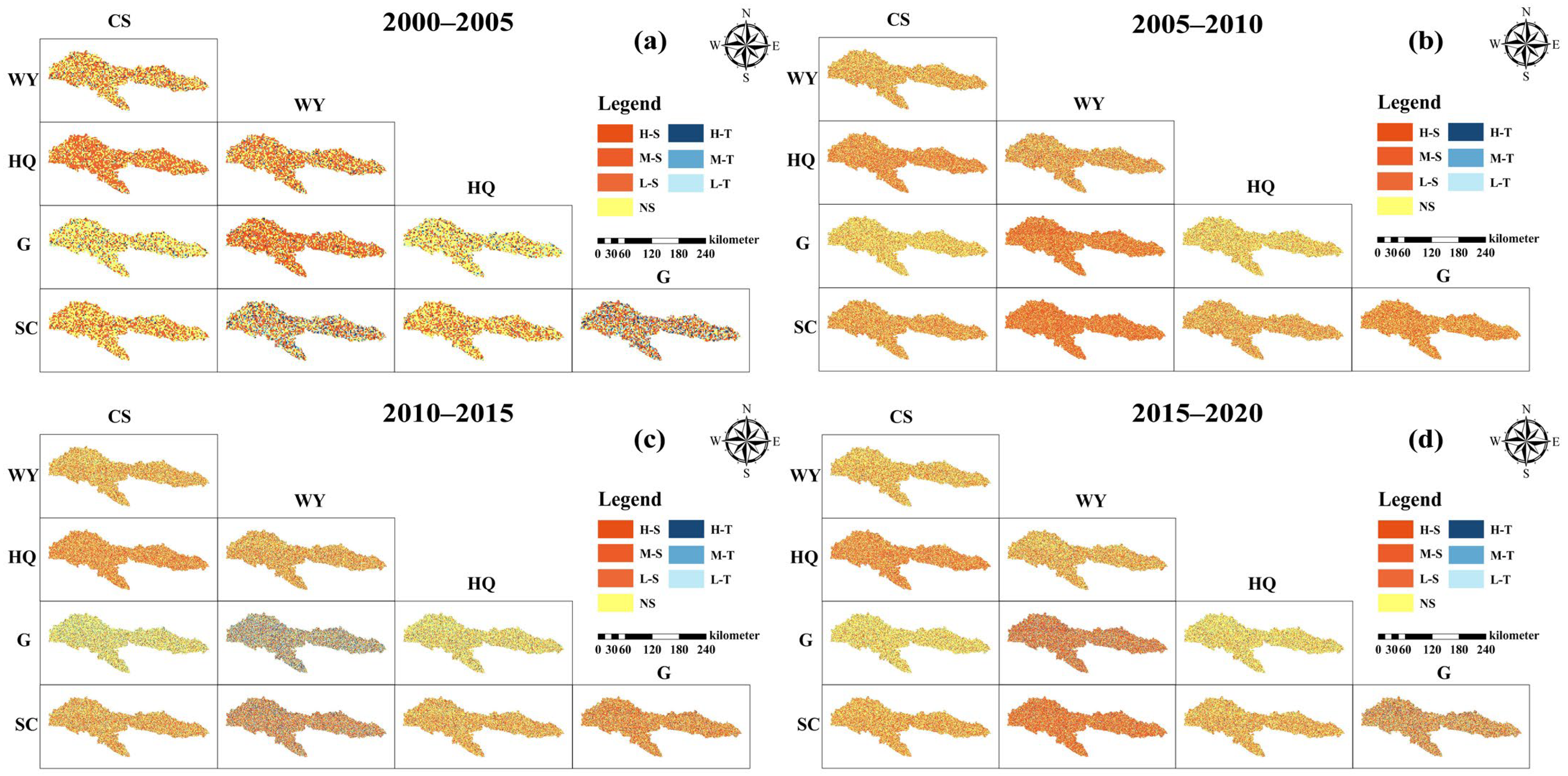
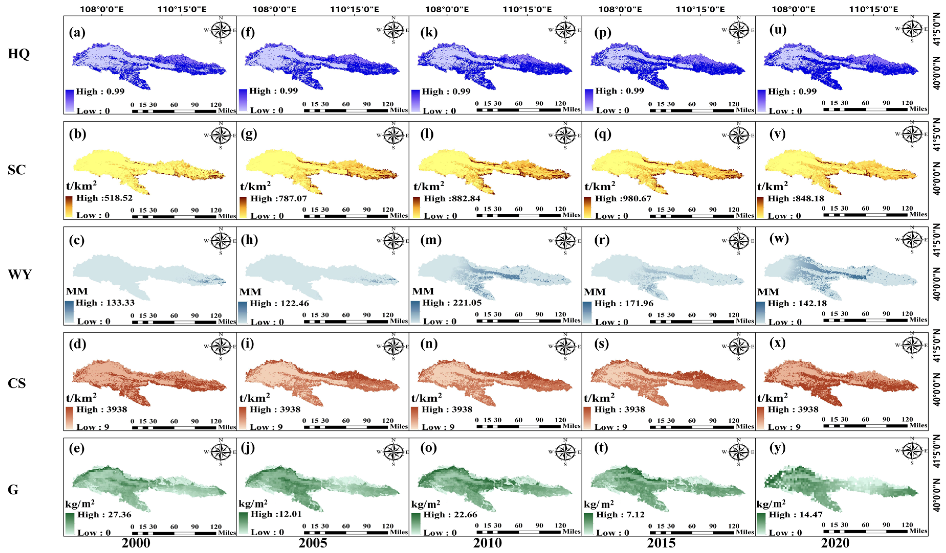
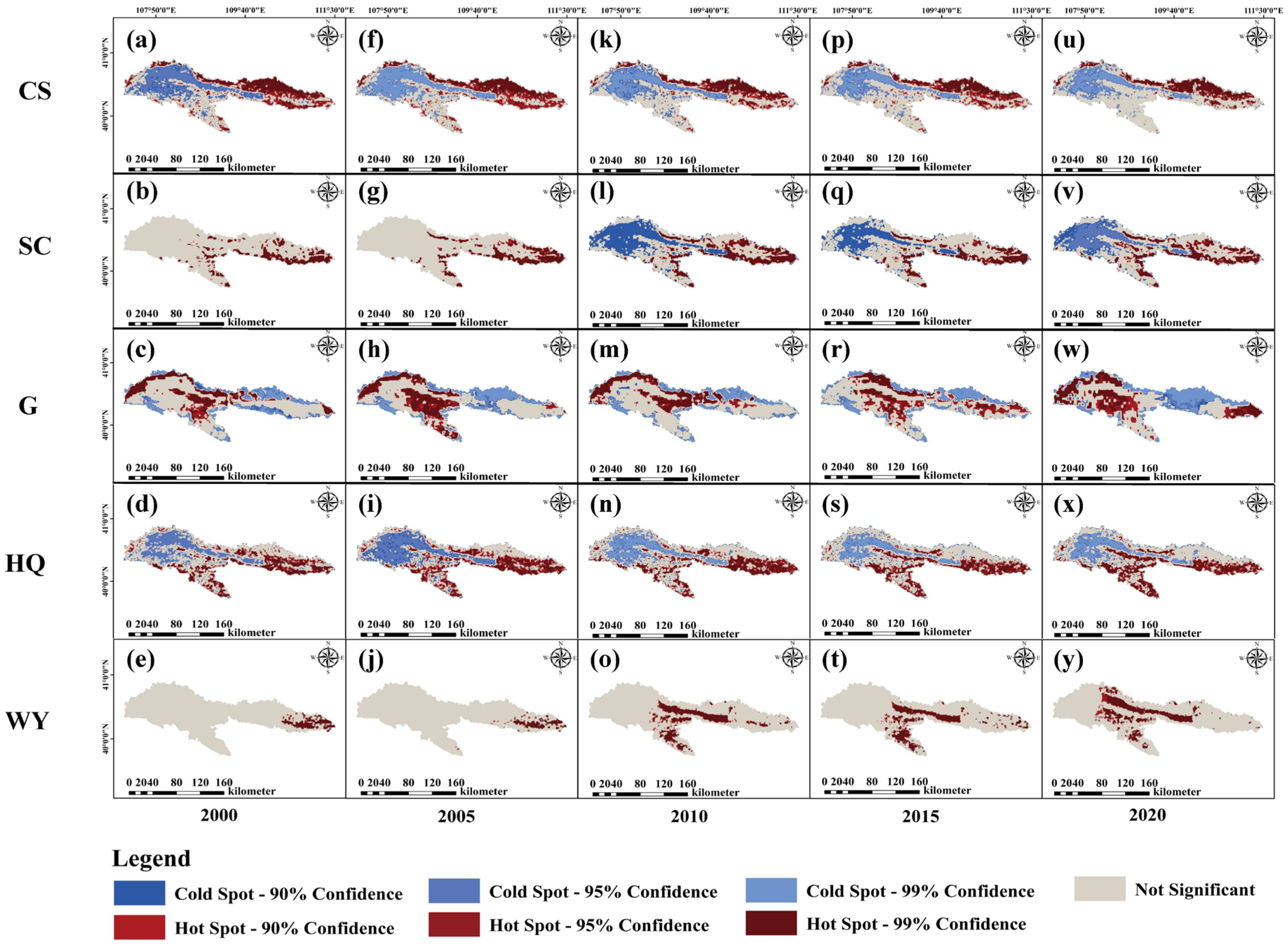
The spatial distribution and clustering patterns of cold and hot spots of different ESs are shown in Figure 4 and Figure 5. From 2000 to 2020, CS showed clear spatial differentiation. High-value areas were concentrated in the north, while medium-value areas formed a narrow belt in the east. Low-value areas were primarily in the central and western parts of the study area. Overall, CS increased from 3.17 × 10⁷ t in 2000 to 3.70 × 10⁷ t in 2020 [

Table 2. The total amounts of the five ESs across different years.

	2000	2005	2010	2015	2020	Unit
HQ	11,070.22	11,443.54	12,055.32	12,497.57	12,522.69	N/A
G	1.466 × 105	7.351 × 104	1.561 × 105	4.345 × 104	8.933 × 104	t
CS	3.173 × 107	3.256 × 107	3.449 × 107	3.650 × 107	3.702 × 107	t
SC	7.970 × 105	1.301 × 106	2.663 × 106	2.21 × 106	2.809 × 106	t
WY	3.413 × 106	2.103 × 106	3.245 × 106	1.159 × 106	3.068 × 106	m3

]. Cold spots were concentrated in the west, and hot spots in the east. Analysis with confidence levels (90%, 95%, 99%) showed that the cold and hot spot areas remained stable, indicating no significant change in the spatial differentiation of CS during the study period.

From 2000 to 2020, the high-value areas of G remained stable in the northwest, while low-value areas were concentrated in the northeast. In terms of temporal variation, total G values exhibited a fluctuating trend, characterized by an ’initial decline followed by recovery’ pattern during both the 2000–2010 and 2010–2020 intervals. Unlike CS, the spatial pattern of the G service’s cold and hot spots showed distinct dynamic evolution. Hot spots were scattered in 2000, expanded in 2005, shrank in 2010, fragmented in 2015, and became patchy in east-west areas in 2020. Cold spots concentrated and shrank in the east (2000–2005), expanded west (2010), then re-expanded east (2020). Insignificant areas fluctuated with them, reflecting the G service’s spatio-temporal heterogeneity in the study area.

SC showed an overall increase, with a slight decline from 2010 to 2015. It rose from 7.97 × 10⁶ t in 2000 to 2.80 × 10⁷ t in 2020 (Table 2). From 2000 to 2005, the study area was dominated by non-significant areas and low-confidence (90%) hot spots, mainly in the central transitional zone. From 2010, cold spots emerged in the west, and between 2010 and 2020, their confidence level gradually increased from 90% to 95%, expanding slightly toward the center. Meanwhile, eastern hot spots’ confidence rose from 90% to 99%, with little change in extent. In summary, the western cold spots’ gradual expansion was the dominant feature of spatial differentiation in SC.

Among the five ESs, WY showed the most noticeable spatio-temporal variability. Total WY values were 3.41 × 10⁶ m³ (2000), 2.10 × 10⁶ m³ (2005), 3.24 × 10⁶ m³ (2010), and 3.06 × 10⁶ m³ (2020), with 2015 being the lowest (Table 2). Spatially, the area was mainly dominated by insignificant regions, with scattered 90% confidence hot spots in the east and no cold spots in the west. After 2010, hot spots rapidly expanded in the central area, covering nearly 40% in 2015 and most of the area by 2020. Meanwhile, the east remained dominated by insignificant areas. The central region’s expanding hot spots were the main feature of spatial differentiation in water conservation services.

During the study period, the spatial distribution of HQ remained generally consistent, showing a slight but continuous upward trend. From 2000 to 2020, the spatial distribution of HQ cold and hot spots exhibited strong stability: cold spots were consistently concentrated in the east, whereas hot spots were in the west. The boundaries between eastern cold spots and western hot spots are closely aligned with the administrative boundaries of the study area (Figure 4). In terms of confidence levels, cold spots in the east consistently remained between the 90% and 95% levels, with no significant spatial expansion, while hot spots in the west persisted between the 95% and 99% levels, with no noticeable contraction. This further confirms the strong spatial stability of HQ during the period.

To summarize, the spatial distribution and temporal dynamics of different ESs exhibit distinct characteristics. CS and HQ showed more stable spatial patterns with consistent hot and cold spots over the study period, whereas G, SC, and WY demonstrated more dynamic changes. G experienced fluctuating trends, with hot spots shifting and shrinking over time, while WY exhibited high temporal variability, particularly with expanding hot spots in the central region after 2010. Additionally, SC showed an overall increase, although spatially, there was significant expansion of cold spots in the western region. These findings highlight the complex, region-specific dynamics of desert ESs, where some services, like CS and HQ, remain stable, while others, like G, SC, and WY, are more sensitive to environmental changes.

3.3. Trade-Offs and Synergies Among ESs

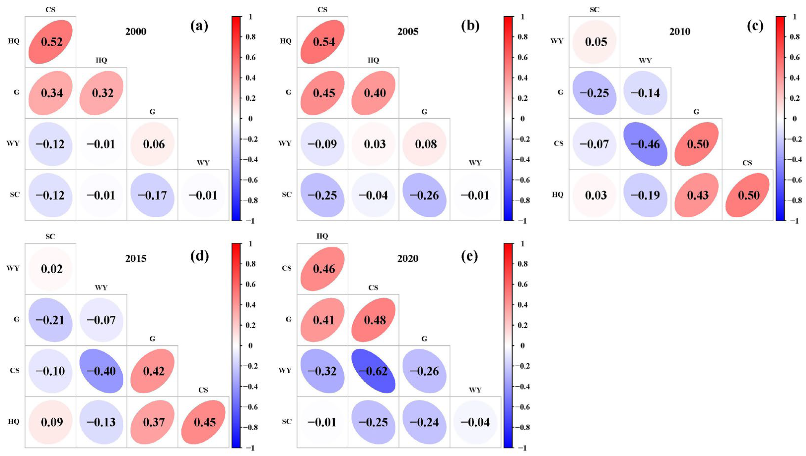
The Spearman correlation method was employed to assess the trade-off and synergy relationships among the five Ess (Figure 6). The results indicate that HQ and CS consistently exhibited a strong synergistic relationship throughout the study period, with correlation coefficients remaining around 0.5 (p < 0.01), suggesting a stable and positive association. In addition, CS demonstrated a high degree of synergy with G, which also implies a significant positive correlation between HQ and G, given their mutual associations with CS. These findings highlight the interlinked nature of these three services in the context of ecological restoration and vegetation improvement. In contrast, WY generally showed a negative correlation with CS, with correlation coefficients consistently exceeding −0.4 (p < 0.01) during the latter half of the study period (2010–2020). Compared to the earlier years (2000 and 2005), the negative correlation between WY and CS became more pronounced, indicating a growing trade-off between these two services over time. SC exhibited a moderately strong trade-off with G, and a weaker negative correlation with CS. These relationships suggest potential competition among services in certain areas, particularly where vegetation structure or land-use practices may favor one service at the expense of another. Finally, no significant correlation was observed between WY and SC across all five time periods, suggesting that these two services operate relatively independently within the ecosystem under study. In summary, HQ and CS consistently showed strong synergy, while WY exhibited an increasing trade-off with CS over time. SC had a moderate trade-off with G and a weaker negative correlation with CS.

Figure 7 shows the spatial distribution of trade-off and synergy relationships among different types of ecosystem services across various periods. From 2000 to 2020, the relationships among ESs were primarily characterized by synergy, with distinct spatial and temporal variations observed across different service combinations. The three service pairs (CS–HQ, CS–SC, HQ–SC) showed a pattern of “strong synergy with continuous enhancement”. Synergistic relationships dominated the study area, with moderate or weak synergy areas being more common in the early period. After 2015, areas with strong synergy expanded rapidly, covering most of the region by 2020. The intensity of synergy increased over time, shifting from a “moderate–weak” to a “strong synergy” stage. No long-term trade-offs or irrelevant relationships disrupted this trend, highlighting the stability of synergistic development.

In contrast, the three service pairs (CS–WY, WY–HQ, and WY–SC) were characterized by “synergy as the dominant relationship with occasional fluctuations”. Although synergy dominated the study area, sporadic patches of trade-off or irrelevance appeared in marginal desert areas and regions with intensive human activity. These non-synergistic patches were scattered and had minimal impact on the overall synergistic pattern. Regionally, synergy intensified from 2000 to 2010, weakened slightly from 2010 to 2015 due to localized disturbances, and recovered after 2015. Synergy remained the prevailing interaction throughout the period.

Beyond these, the four service pairs (CS–G, WY–G, HQ–G, G–SC) showed weak interactions with gradual temporal variation. Spatially, most of the study region was dominated by irrelevant relationships, with small patches of weak synergy or trade-off. No contiguous areas of strong interaction were observed, indicating low spatial aggregation. Temporally, the interaction intensity remained low from 2000 to 2020. Irrelevant areas slightly decreased, while weak synergy or trade-off areas increased, signaling a shift from “near non-interaction” to “localized weak interaction”.

3.4. Driving Mechanism of ESs

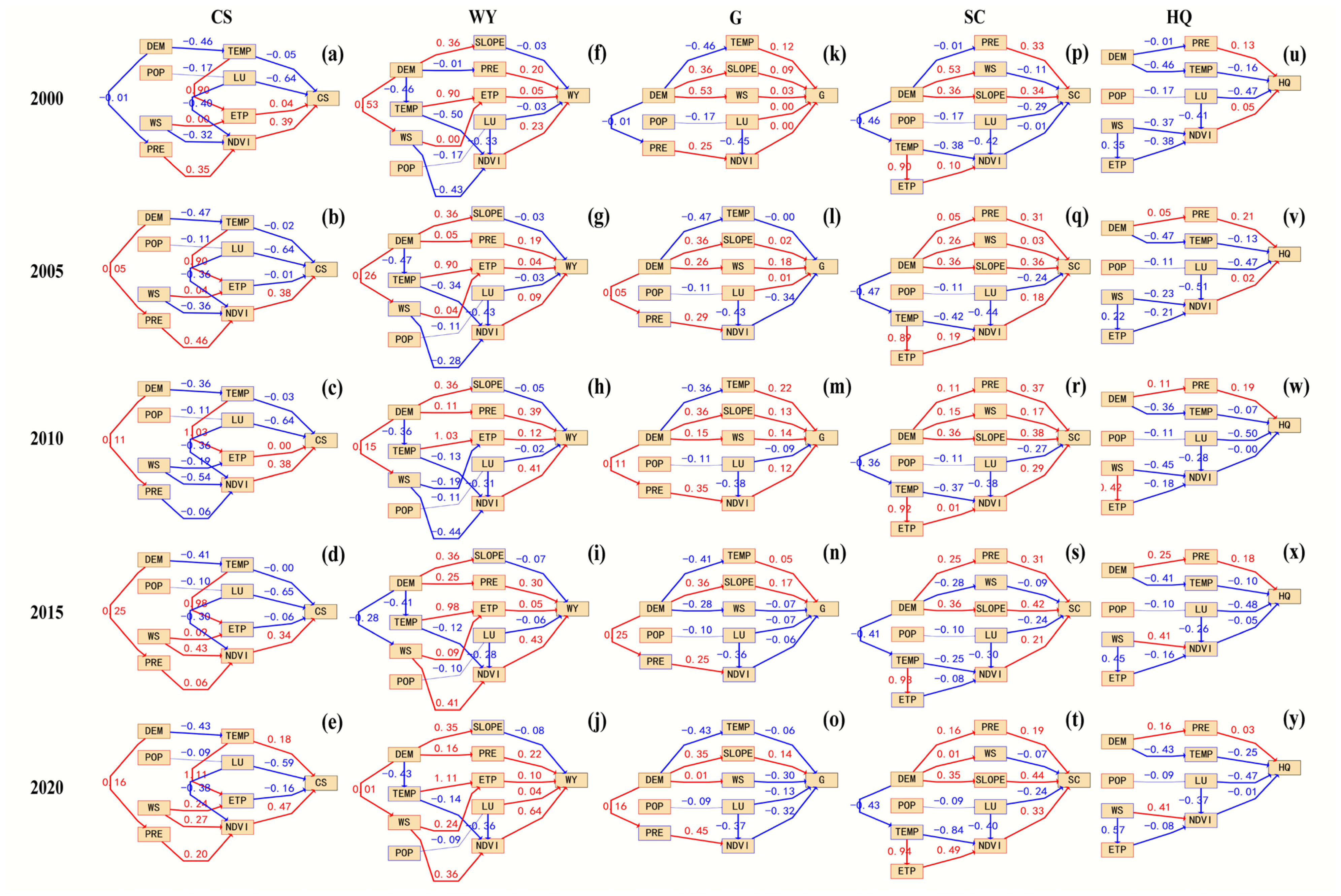
The evaluation of the structural equation model indicates that all endogenous latent variables achieved satisfactory explanatory power, with their coefficients of determination (R²) showing a consistent increasing trend over the study period (the average R² rose from 0.256 in 2000 to 0.402 in 2020). Furthermore, bootstrap-based tests of path significance supported most hypothesized relationships (with 94.1% of paths being significant in the 2020 model). Together, these results demonstrate that the overall model quality is robust and sufficient for further mechanistic interpretation. Figure 8 illustrates the driving mechanisms of different ESs in different periods. From 2000 to 2020, LU consistently had a strong negative effect on CS, with this relationship remaining stable throughout the study period. This indicates that changes in land types continuously constrained CS, although the inhibitory effect slightly slowed by 2020. In contrast, ETP showed a weak negative effect, mildly limiting CS. Additionally, the correlation pathways of several factors varied over time. In 2000, LU, PRE, and WS had a pronounced indirect effect on NDVI, subsequently influencing CS. Among these, WS’s influence on NDVI fluctuated significantly. Overall, the driving mechanism of CS had two key features: (1) core factors like LU and vegetation continuously regulated CS, and (2) dynamic changes in other factors reshaped the driving relationships.

PRE and NDVI consistently exerted significant positive effects on WY during the study period, with the effect of PRE being more stable than that of NDVI. Other factors, such as LU and ETP, showed weak correlations with WY, and their magnitude of change was limited. A prominent impact pathway was identified wherein variations in TEMP affected the ETP rate, which in turn influenced WY. Notably, the effects of WS on NDVI and ETP fluctuated considerably, indirectly contributing to changes in regional WY.

Natural factors such as TEMP, SLOPE, and WS, along with anthropogenic and ecological factors like LU and NDVI, jointly influenced grain production (G) from 2000 to 2020, forming its core driving system. However, the relationships between these factors and G exhibited varying degrees of dynamic complexity. Based on the characteristics of key drivers, WS’s effect on G can be divided into three phases: weak promotion (2000–2010), weak interference (2010–2015), and strong interference (2015–2020). In contrast, NDVI’s effect on G was pronounced only during 2010–2020, while it remained insignificant in other periods. Apart from WS and NDVI, other factors had weaker direct effects on G. The indirect effects of terrain variables (SLOPE and DEM) on TEMP and WS, and the influence of PRE on NDVI, were the most prominent indirect relationships throughout the study period, remaining stable without large fluctuations, providing consistent support for G’s driving mechanism.

PRE, terrain, and NDVI were key driving factors for SC from 2000 to 2020, with PRE, SLOPE, and NDVI exerting stable positive effects, while LU maintained a steady interfering effect. These relationships formed the core direct impact framework of SC’s driving mechanism, characterized by stability and directionality. Indirectly, only the LU–NDVI and TEMP–ETP pathways remained stable, indicating strong temporal variability in SC’s indirect driving pathways. Notably, the TEMP–NDVI pathway intensified sharply by 2020, with its path coefficient rising to –0.84, indicating that the negative influence of TEMP on NDVI was strengthened, altering the positive effect of NDVI on SC through the TEMP–NDVI–SC pathway. This shift became a defining feature of SC’s driving mechanism in 2020.

Throughout the entire study period, TEMP and LU consistently exerted interfering effects on HQ, although their stabilities differed markedly. The path coefficient of LU’s interfering effect on HQ remained steady without major fluctuations, whereas TEMP’s interference varied significantly, exhibiting strong temporal dynamics. PRE maintained a moderate-to-low positive effect on HQ across all periods, though its intensity varied over time. In 2020, the path coefficient of PRE’s impact on HQ reached its lowest level of the entire study period, marking a key transition point in its functional influence. Regarding indirect pathways, the coefficients of the WS–NDVI and WS–ETP–NDVI chains fluctuated considerably over time, indicating that the influence of WS on HQ was highly time-dependent. By contrast, the coefficients of the POP–LU, LU–NDVI, and DEM–TEMP pathways showed no substantial changes across the study period, reflecting stable and persistent relationships. Overall, while HQ’s driving mechanism incorporated several dynamically changing pathways, its core indirect relationships remained robust and stable, maintaining a relatively steady driving framework throughout the 20-year period.

4. Discussion

4.1. Spatio-Temporal Dynamics of LU

LU in the KBQ Desert has undergone remarkable transformations over the past two decades. A series of ecological restoration initiatives have led to a consistent decline in shifting sand, much of which has been converted into grassland. Consequently, grassland has become the dominant LU type in the region, aligning well with findings from previous studies [33,34]. Meanwhile, urban land has expanded nearly fivefold during the study period, reflecting the increasing pressure of rapid urbanization. Both cropland and water have also increased, likely driven by POP growth and the implementation of regional environmental protection policies.

Extensive research has underscored the positive impacts of large-scale ecological restoration programs, particularly regarding vegetation recovery and CS. Xu et al. [35] demonstrated that initiatives such as the Three-North Shelter Forest Program and the Grain-for-Green Program have substantially increased vegetation cover across northern China, thereby enhancing regional CS capacity. These restoration efforts have played a crucial role in combating desertification, as evidenced by improvements in ESs such as water purification, surface runoff regulation, and carbon accumulation [36,37,38].

However, a growing body of literature also points to the significant challenges associated with large-scale afforestation efforts in arid and semi-arid regions. Qi et al. [10] reported that, compared with shrubs, forests tend to exhibit lower survival rates and faster degradation in sandy environments, leading to a reduced contribution to desertification control. Similarly, Wang et al. [39] found that newly planted tree species often consume more water than native vegetation, exacerbating water scarcity in already water-limited ecosystems. Moreover, Cao et al. [40] emphasized that overreliance on afforestation in China’s arid regions has frequently produced suboptimal outcomes, suggesting that drought- and cold-tolerant vegetation such as shrubs and grasses may be more suitable in areas with low PRE (<250 mm).

The current LU results corroborate these findings: forested land accounts for less than 0.01% of the total area, indicating that forests are not a dominant land type in the KBQ Desert. Instead, local desertification control strategies primarily rely on various sand-fixation techniques (e.g., straw checkerboards) combined with the use of cold- and drought-tolerant grass species [39]. Despite these efforts, a considerable portion of sandy land in the KBQ Desert remains in need of appropriate management to curb desertification and improve vegetation survival rates.

4.2. Changes in ESs

Previous studies have clearly demonstrated that the implementation of ecological restoration projects can substantially enhance multiple ESs [26,35,41,42]. Consistent with these findings, this study reveals that the five key ESs in the KBQ Desert exhibited an overall increasing trend from 2000 to 2020. However, their trajectories displayed distinct spatio-temporal variations, closely linked to the progress of ecological restoration, local environmental conditions, and human activities.

For CS, continuous increases in vegetation cover over the study period led to a steady rise in total CS—from 3.17 × 10⁷ t in 2000 to 3.70 × 10⁷ t in 2020. This pattern supports previous conclusions that “an increase in the proportion of forests and grasslands directly promotes CS” [37,38,41]. Spatially, CS maintained a consistent pattern of “hotspot in the east and coldspot in the west”. The eastern region, near the Yellow River and with a relatively high groundwater level, provided favorable conditions for vegetation growth, resulting in strong CS capacity. In contrast, the western inland dune area, where vegetation coverage remained below 5%, showed persistently low CS values.

Similar to CS, the improvement and spatial stability of HQ were primarily driven by enhanced vegetation cover [43]. HQ displayed a modest yet steady upward trend, with a spatially stable distribution of “hotspots in the east and coldspots in the west”. The western area, designated as a core ecological protection zone, experienced minimal agricultural or urban disturbance and thus maintained high habitat integrity. Conversely, the eastern region, dominated by cropland and urban land, suffered from severe habitat fragmentation and remained a long-term coldspot. Together, these two services—CS and HQ—underscore the pivotal role of vegetation restoration in promoting synergistic improvements within the “CS–HQ” system.

SC showed a pronounced overall increase, with total soil retention rising from 7.97 × 10⁶ t to 2.80 × 10⁷ t, despite a minor decline between 2010 and 2015 [44]. Spatially, the expansion of coldspot areas in the western region was the defining feature. The overall improvement in SC can largely be attributed to vegetation recovery, where plant roots strengthened soil structure and the litter layer reduced the impacts of raindrops and surface runoff, thus mitigating erosion [45,46]. The temporary decline during 2010–2015 was likely due to extreme PRE, with intense rainfall exceeding the soil retention capacity of the vegetation and thus temporarily increasing erosion [15]. The gradual expansion of low-value SC areas in the western region (confidence level rising from 90% to 95%) was primarily due to the fragile ecological base of this dune-dominated landscape. Even after restoration efforts, thin soil layers and sparse vegetation coverage continued to limit erosion resistance, allowing low-SC zones to extend gradually toward the central region.

Both G and WY exhibited more complex and dynamic patterns [47,48]. G experienced cyclical “decline–recovery” fluctuations during both 2000–2010 and 2010–2020, driven largely by changes in WS and the varying effectiveness of sand-fixation measures [48,49]. WY, identified as the most spatio-temporally variable service among the five, reached its lowest level in 2015, with changes primarily governed by PRE [50]. The years 2005 and 2015 were regional drought years characterized by reduced soil moisture and lower vegetation transpiration, directly leading to a decline in WY. By 2020, however, WY exhibited a remarkable spatial shift, with “hotspots emerging and expanding across the central region”. This unique phenomenon in the KBQ Desert can be attributed to a combination of factors: recovery of PRE levels in the west and the widespread adoption of efficient irrigation techniques, such as drip and sprinkler systems, in artificial oases [50]. These irrigation practices not only replenished soil moisture but also enhanced vegetation growth, thereby improving the water-retention capacity of local ecosystems and promoting an overall increase in WY [43,50].

Compared with other arid regions such as the Tengger Desert, the dynamics of ESs in the KBQ Desert showed some differences. The steady enhancement of CS and HQ, the fluctuating yet resilient recovery of G, and the regional optimization of WY were all closely associated with ecological engineering efforts, including the Three-North Shelterbelt Program, artificial afforestation, and sand barrier-based stabilization techniques. In contrast, ES changes in other arid zones are often dominated by natural environmental variability (e.g., PRE fluctuations). Meanwhile, the significant and sustained improvement of SC in the KBQ Desert reflects the targeted and effective implementation of SC strategies, providing valuable practical insights for ecological restoration in similar desert ecosystems.

4.3. Variations in the Correlational Relationships Among ESs

Spearman correlation and spatial pattern analyses revealed that synergy was the dominant form of interaction among the five ESs in the KBQ Desert between 2000 and 2020, although the intensity and stability of these relationships varied considerably across different service pairs.

The three service pairs, CS–HQ, CS–SC, and HQ–SC, displayed the characteristic of “strong synergy with continuous intensification” [43,51]. The underlying mechanism lies in their shared dependence on vegetation coverage. Vegetation growth enhances CS through biomass accumulation, improves HQ by optimizing microhabitats (e.g., providing habitats and purifying the environment), and strengthens SC through root stabilization and the reduction of surface runoff [45,46]. With the progressive implementation of ecological restoration projects in the KBQ Desert, vegetation coverage increased steadily, reinforcing the synergistic relationships among these three services [43,51]. Consequently, the dominant interaction mode transitioned from moderate and weak synergy to strong synergy. Throughout the entire study period, no significant trade-offs or irrelevant disturbances were observed, reflecting the effectiveness of regional restoration efforts in achieving “multi-service synergistic gains” [52]. This finding aligns with previous studies that reported intensified CS–SC–HQ synergy following vegetation restoration in the Mu Us Sandy Land, confirming the widespread presence of this synergistic pattern in arid and semi-arid sandy ecosystems.

In contrast, another three service pairs, CS–WY, WY–HQ, and WY–SC, exhibited the trait of “synergy as the dominant trend with occasional fluctuations,” reflecting the complex coupling between WY and the other services [43]. The overall synergistic relationships originate from the positive influence of water availability on vegetation growth, which in turn enhances CS, HQ, and SC [50,52]. However, small and scattered trade-off patches emerged in certain marginal or human-disturbed areas, likely due to localized water scarcity. In such regions, increased water consumption by vegetation to support CS and SC may reduce surface runoff, thereby diminishing WY. The observed “intensification–fluctuation–reintensification” pattern of synergy, with a brief decline during 2010–2015, corresponds to PRE variability [15,50]. The relatively dry conditions during that period intensified competition for water resources, temporarily weakening synergistic interactions; after 2015, the recovery of PRE led to renewed strengthening of synergy.

The four service pairs (CS–G, WY–G, HQ–G, G–SC) showed weak interactions with gradual variation, primarily driven by WS and terrain, rather than vegetation [47,48]. Vegetation contributes to sand fixation, but its effect is secondary to wind dynamics, resulting in weak correlations between G and other services [48,49]. From 2000 to 2020, these service pairs evolved from near non-interaction to localized weak interaction, likely due to improved vegetation cover [43,51]. Vegetation’s regulatory role in sand fixation became more evident, forming patches of weak synergy or trade-off. A pronounced trade-off between WY and CS emerged after 2010, with correlation coefficients falling below –0.4, likely due to increased vegetation cover, which raised transpiration and water consumption, reducing surface runoff and WY. This trade-off may constrain the simultaneous enhancement of WY and CS in water-limited desert ecosystems [15]. Future management should focus on mitigating this conflict by introducing drought-tolerant species and optimizing vegetation structure [50,52].

4.4. Dynamics of Driving Mechanisms

From 2000 to 2020, the driving mechanisms of the five ESs in the KBQ Desert exhibited a characteristic pattern of “stable core factors + dynamic secondary factors”. Natural factors (PRE, TEMP, WS) and anthropogenic factors (LU, ecological engineering) interacted to jointly shape the dynamics of ESs [52]. This process aligns well with the “Driver–Pressure–State–Impact–Response” (DPSIR) framework widely applied in ecosystem management.

The core driving factors of CS were LU and NDVI [43,50]. LU exerted a consistently strong negative effect over the long term, while NDVI played a positive regulatory role. The negative influence of LU slightly weakened in 2020, likely due to land-use optimization, for example, the conversion of large areas of shifting sand into grassland. ETP imposed a weak negative effect on CS because high ETP induces water stress that inhibits vegetation growth and thus reduces carbon accumulation. Dynamic secondary factors such as WS and PRE influenced CS indirectly through NDVI [52]. For instance, in 2000, the indirect effects of WS and PRE on NDVI were significant: high WS damaged young vegetation, whereas sufficient PRE promoted plant growth [34,43]. The pronounced fluctuations in WS’s effect on NDVI underscore vegetation’s high sensitivity to wind in desert environments [47,48].

The driving forces of sand fixation (G) were primarily governed by the synergistic interactions between natural factors (TEMP, SLOPE, WS) and anthropogenic factors (LU, NDVI), among which WS and NDVI were the key dynamic drivers [47,48]. The effect of WS on G evolved through three stages: promotion → weak interference → strong interference [48]. From 2000 to 2010, WS was relatively low, and vegetation together with sand barriers exerted a weak promoting effect [49]. After 2010, increasing WS exceeded the capacity of sand-fixation measures, turning it into an interfering factor, which became even stronger by 2020 [46,47]. NDVI showed a strong interfering effect on G only between 2010 and 2020, likely because of poor vegetation survival, as vegetation failed to stabilize sand effectively, leading to a decrease in overall G [43,51]. Two stable indirect pathways, namely terrain → TEMP/WS and PRE → NDVI, provided continuous support for G’s driving mechanism. Terrain indirectly enhanced G by reducing WS and moderating TEMP, while PRE promoted vegetation growth, indirectly stabilizing G [50,52]. This implies that even when direct drivers like WS fluctuate, these indirect pathways can help maintain the overall stability of the sand-fixation mechanism [43].

For SC, PRE, terrain, and LU were the main influencing factors, each exerting stable and direct effects [52]. PRE and slope acted positively, as adequate PRE stimulates vegetation growth, while moderate slopes reduce runoff velocity, jointly enhancing SC [45,46]. In contrast, LU had a stable negative influence: cropland and urban land, characterized by low vegetation cover and high surface disturbance, intensified soil erosion [51]. Apart from the “LU–NDVI” and “TEMP–ETP” pathways, no other stable indirect pathways were identified, indicating that the SC driving process is relatively direct with few mediating links. In 2020, the negative effect of the “TEMP–NDVI” pathway was notably strengthened, with a path coefficient reaching −0.84. This suggests that extreme heat that year greatly increased water stress, inhibited vegetation growth, and consequently weakened plants’ soil-stabilizing capacity, highlighting the vulnerability of SC to climate change.

The core positive driving factors of WY were PRE and NDVI, with PRE exerting the more stable effect [50]. PRE directly enhanced WY by increasing surface runoff, whereas NDVI had a dual effect: moderate vegetation cover reduced runoff loss and increased WY, while excessive vegetation reduced WY through higher transpiration water consumption [43]. The indirect “TEMP–ETP–WY” pathway was a key regulating link: rising TEMP elevated ETP, thereby reducing soil moisture and runoff. Fluctuations in WS also indirectly influenced WY by affecting NDVI and ETP, as strong WS increased ETP and damaged vegetation, jointly producing a pronounced negative effect on WY. The complexity of these interactions explains why WY exhibited the greatest spatio-temporal variability among all Ess [43].

The core interfering drivers of HQ were TEMP and LU, with LU exerting a stable negative influence [51]. The interfering effect of TEMP, however, showed dynamic fluctuations over time, with extreme heat and cold both degrading HQ. PRE had a moderate positive effect by improving vegetation cover and water availability, thereby indirectly optimizing HQ [43,52]. Indirect pathways such as POP → LU and LU → NDVI also played important roles: POP growth drove land-use changes (e.g., cropland expansion), which affected NDVI and ultimately altered regional HQ [39,51].

Overall, the driving mechanisms of ESs in the KBQ Desert underscore the crucial regulatory role of anthropogenic factors, particularly land-use change and ecological engineering, while natural factors remain the fundamental determinants [51]. Notably, recent improvements in ESs have been predominantly driven by human intervention, confirming the effectiveness of ecological restoration efforts in the KBQ Desert and offering a replicable model for enhancing ESs in other arid regions [43,53].

4.5. Research Implications for Sand Regions

The dynamics of ESs in desert and semi-arid regions, such as the KBQ Desert, hold significant ecological and practical importance for both regional sustainability and global ecological restoration efforts. This study unveils the driving mechanisms behind ESs, with broad implications for ecological restoration strategies, particularly for desert ecosystems in other regions. These regions face similar challenges, including desertification, water scarcity, and land degradation, making the findings of this study highly relevant for guiding restoration strategies in these areas.

A key finding of this study is the significant trade-off between WY and CS, which emerges as a central challenge for regional sustainable development. This trade-off underscores a critical, broader question: the long-term sustainability of the ongoing expansion of cropland and grassland in the KBQ Desert. While this LU transformation has effectively enhanced multiple ESs in the short term, its persistence is threatened by the inherent vulnerabilities of arid ecosystems. First, intensifying water competition between agricultural use and ecological needs may jeopardize the water security essential for maintaining restored vegetation. Second, the potential homogenization of landscapes into large-scale monocultures could erode local biodiversity and reduce ecosystem resilience, increasing susceptibility to climate extremes and economic shifts. Third, unsustainable agricultural practices risk triggering long-term soil degradation, including salinization and nutrient depletion. Therefore, future ecological management must undergo a fundamental paradigm shift from pursuing sheer area expansion to fostering ecological quality, adaptive capacity, and sustainable intensification. Adaptive strategies should integrate: (1) water-smart practices, such as efficient irrigation and the cultivation of drought-tolerant species, to mitigate the WY-CS trade-off; (2) the promotion of diverse, native planting schemes to maintain ecological integrity and buffer against disturbances; and (3) the establishment of robust, science-informed monitoring and policy frameworks that dynamically balance agricultural production with the conservation of critical, regulating ESs. Insights into key pathways—such as PRE → NDVI → ES and LU → NDVI → ES—provided by the PLS-PM analysis, are invaluable for tailoring these strategies to local climatic and vegetation dynamics, not only in the KBQ Desert but also in other desertified regions facing similar sustainability dilemmas.

4.6. Limitation

Although this study has revealed the spatio-temporal characteristics of ESs in the KBQ Desert to some extent, the precision of the foundational data obtained is limited, preventing a comprehensive description of the ESs’ spatio-temporal distribution patterns at a finer scale. For instance, the accuracy of LU data products and other gridded data products is generally not high enough to capture the detailed variations within the region. On the other hand, this study did not differentiate between the growing season and the non-growing season to investigate the dynamic changes of the KBQ Desert. The natural landscape in this region varies significantly between different seasons. Therefore, the next phase could consider dividing each year into various periods for the analysis of ES characteristics. For instance, G services may fluctuate due to factors such as vegetation and WS in different seasons, leading to significant differences in assessment outcomes.

Additionally, this study didn’t forecast the trends in ES changes under various future scenarios for the KBQ Desert. Given that ecological restoration projects are long-term endeavors, especially under the challenging conditions of fragile desert ecosystems, ongoing monitoring and adjustment over extended periods are indispensable. Therefore, our next steps will involve exploring and modeling the dynamic characteristics of ESs in the KBQ Desert under different future scenarios, aiming to provide more comprehensive scientific evidence for future regional management planning.

5. Conclusions

This research carries out a clear exploration and analysis of the LU changes, the evolution of the spatio-temporal patterns of ESs, and the relationships among them in the KBQ Desert and clarifies the driving mechanisms behind the changes of various ESs. Sandy areas, cropland, and grassland together accounted for over 95% of the total area and underwent the most significant changes between 2000 and 2020. Notably, sand areas decreased by 2697 km², while grassland and cropland increased by 1864 km² and 519 km², respectively, primarily through the conversion of sand to grassland. HQ, WY, CS, and SC all exhibited a trend of positive growth, whereas G showed fluctuations. The expansion of grassland and cropland was the main contributor to the improvement of these services, which indicates that regional ecosystem restoration projects have played a certain role in promoting the improvement of the overall ecological environment. Among the various ESs in the KBQ Desert, the synergistic relationships between CS and HQ, and between CS and G, stand out the most when viewed from the angle of spatio-temporal holistic connections. In contrast, the relationship between WY and other services is dominated by trade-offs. Furthermore, the results of spatial relationships indicate that all pairs of services also exhibit the distinct characteristic of “predominantly synergistic” in most areas, while trade-off occurs in local regions.

Based on the findings from exploring the driving mechanisms of various ESs, it is evident that the application of Partial Least Squares Path Modeling (PLS-PM) has effectively revealed the driving mechanisms of ESs in the KBQ Desert. PLS-PM provides a more comprehensive analysis of the nonlinear interactions and indirect effects between multiple drivers, which traditional methods often fail to capture. By uncovering latent pathways and multi-step causal chains, it also offers valuable insights into the driving mechanisms behind changes in ESs, mechanisms that have often been overlooked in previous research. From the results of the analysis of driving mechanisms, PRE, NDVI, and LU are the primary driving factors influencing changes in each service. In contrast, other factors act on these services through indirect pathways, among which interactions such as TEMP–ETP and PRE–NDVI have the most significant impacts on ES changes. This indicates that the influence of anthropogenic factors on the KBQ Desert ecosystem remains relatively limited, mainly manifesting as effects on LU changes; this aligns with the region’s characteristic of low POP. Meanwhile, natural factors remain the primary drivers of changes in regional ESs.

References

1. Huang, J.; Yu, H.; Dai, A.; Wei, Y.; Kang, L. Drylands face potential threat under 2 °C global warming target. Nat. Clim. Chang. 2017, 7, 417–422. [Google Scholar] [CrossRef] [Scilit]
2. Seddon, A.W.R.; Macias-Fauria, M.; Long, P.; Benz, D.; Willis, K.J. Sensitivity of global terrestrial ecosystems to climate variability. Nature 2016, 531, 229–232. [Google Scholar] [CrossRef] [Scilit] [PubMed]
3. Arunyawat, S.; Shrestha, R.P. Assessing land use change and its impact on ecosystem services in Northern Thailand. Sustainability 2016, 8, 768. [Google Scholar] [CrossRef] [Scilit]
4. Pham, H.V.; Sperotto, A.; Torresan, S.; Acuna, V.; Jorda-Capdevila, D.; Rianna, G.; Marcomini, A.; Critto, A. Coupling scenarios of climate and land-use change with assessments of potential ecosystem services at the river basin scale. Ecosyst. Serv. 2019, 40, 101045. [Google Scholar] [CrossRef] [Scilit]
5. Zhang, Y.; Lu, X.; Liu, B.; Wu, D.; Fu, G.; Zhao, Y.; Sun, P. Spatial relationships between ecosystem services and socioecological drivers across a large-scale region: A case study in the Yellow River Basin. Sci. Total Environ. 2021, 766, 142480. [Google Scholar] [CrossRef] [Scilit]
6. Hasan, S.S.; Zhen, L.; Miah, M.G.; Ahamed, T.; Samie, A. Impact of land use change on ecosystem services: A review. Environ. Dev. 2020, 34, 100527. [Google Scholar] [CrossRef] [Scilit]
7. Liu, M.; Wei, H.; Dong, X.; Wang, X.; Zhao, B.; Zhang, Y. Integrating land use, ecosystem service, and human well-being: A systematic review. Sustainability 2022, 14, 6926. [Google Scholar] [CrossRef] [Scilit]
8. Lawler, J.J.; Lewis, D.J.; Nelson, E.; Plantinga, A.J.; Polasky, S.; Withey, J.C.; Helmers, D.P.; Martinuzzi, S.; Pennington, D.; Radeloff, V.C. Projected land-use change impacts on ecosystem services in the United States. Proc. Natl. Acad. Sci. USA 2014, 111, 7492–7497. [Google Scholar] [CrossRef] [Scilit]
9. Nunes, A.; Oliveira, G.; Mexia, T.; Valdecantos, A.; Zucca, C.; Costantini, E.A.; Abraham, E.M.; Kyriazopoulos, A.P.; Salah, A.; Prasse, R.; et al. Ecological restoration across the Mediterranean Basin as viewed by practitioners. Sci. Total Environ. 2016, 566–567, 722–732. [Google Scholar] [CrossRef] [Scilit]
10. Qi, K.; Zhu, J.; Zheng, X.; Wang, G.; Li, M. Impacts of the world’s largest afforestation program (Three-North Afforestation Program) on desertification control in sandy land of China. GISci. Remote Sens. 2023, 60, 2167574. [Google Scholar] [CrossRef] [Scilit]
11. Bryan, B.A.; Gao, L.; Ye, Y.; Sun, X.; Connor, J.D.; Crossman, N.D.; Stafford-Smith, M.; Wu, J.; He, C.; Yu, D.; et al. China’s response to a national land-system sustainability emergency. Nature 2018, 559, 193–204. [Google Scholar] [CrossRef] [Scilit]
12. Zeng, L.; Li, J.; Zhou, Z.; Yu, Y. Optimizing land use patterns for the Grain for Green Project based on the efficiency of ecosystem services under different objectives. Ecol. Indic. 2020, 114, 106347. [Google Scholar] [CrossRef] [Scilit]
13. Li, Z.; Cheng, X.; Han, H. Future impacts of land use change on ecosystem services under different scenarios in the ecological conservation area of Beijing, China. Forests 2020, 11, 584. [Google Scholar] [CrossRef] [Scilit]
14. Song, S.; Chen, X.; Hu, Z.; Zan, C.; Liu, T.; De Maeyer, P.; Sun, Y. Deciphering the impact of wind erosion on ecosystem services: An integrated framework for assessment and spatiotemporal analysis in arid regions. Ecol. Indic. 2023, 154, 110693. [Google Scholar] [CrossRef] [Scilit]
15. Luo, S.; Luo, Z. Spatial differentiation and associated factors of non-grain cultivated land in mineral grain composite area considering scale effects. Trans. Chin. Soc. Agric. Eng. 2024, 40, 265–275. [Google Scholar]
16. Li, Y.; Zhang, L.; Yan, J.; Wang, P.; Hu, N.; Cheng, W.; Fu, B. Mapping the hotspots and coldspots of ecosystem services in conservation priority setting. J. Geogr. Sci. 2017, 27, 681–696. [Google Scholar] [CrossRef] [Scilit]
17. Zhang, J.; Zhang, Z.; Liu, L.; Cao, Y.; Zhang, M.; Yuan, Z.; Ma, R.; Liu, X.; Liu, Y. Scaling effects of ecosystem service trade-off and synergy in arid inland river basins: A case study of the Manas River Basin of Xinjiang, China. Ecol. Indic. 2025, 173, 113358. [Google Scholar] [CrossRef] [Scilit]
18. Chen, H.; Costanza, R. Valuation and management of desert ecosystems and their services. Ecosyst. Serv. 2024, 66, 101607. [Google Scholar] [CrossRef] [Scilit]
19. Yang, J.; Huang, X. The 30 m annual land cover dataset and its dynamics in China from 1990 to 2019. Earth Syst. Sci. Data 2021, 13, 3907–3925. [Google Scholar] [CrossRef] [Scilit]
20. Peng, S.; Ding, Y.; Wen, Z.; Chen, Y.; Cao, Y.; Ren, J. 1-km Monthly Potential Evapotranspiration Dataset for China (1901–2022). National Tibetan Plateau/Third Pole Environment Data Center. Available online: https://data.tpdc.ac.cn/en/data/8b11da09-1a40-4014-bd3d-2b86e6dccad4/ (accessed on 15 January 2026).
21. Sims, K.; Reith, A.; Bright, E.; Kaufman, J.; Pyle, J.; Epting, J.; Gonzales, J.; Adams, D.; Powell, E.; Urban, M.; et al. LandScan Global 2022; Oak Ridge National Laboratory: Oak Ridge, TN, USA, 2023. Available online: https://landscan.ornl.gov/ (accessed on 15 January 2026).
22. FAO; IIASA; ISRIC; ISSCAS; JRC. Harmonized World Soil Database (HWSD), Version 1.2. Available online: https://www.fao.org/soils-portal/soil-survey/soil-maps-and-databases/harmonized-world-soil-database-v12/en/ (accessed on 15 January 2026).
23. China Meteorological Administration. Daily Dataset of Surface Meteorological Observations in China (V3.0) [Data set]; China Meteorological Data Service Center: Beijing, China, 2020. [Google Scholar]
24. Liang, Y.; Liu, L. An integrated ecosystem service assessment in an artificial desert oasis of northwestern China. J. Land Use Sci. 2017, 12, 154–167. [Google Scholar] [CrossRef] [Scilit]
25. Hamel, P.; Guswa, A.J. Uncertainty analysis of a spatially explicit annual water-balance model: Case study of the Cape Fear basin, North Carolina. Hydrol. Earth Syst. Sci. 2015, 19, 839–853. [Google Scholar] [CrossRef] [Scilit]
26. Muyibul, Z. Trade-offs and synergies between ecosystem services in Yutian County along the Keriya River Basin, Northwest China. J. Arid Land 2024, 16, 943–962. [Google Scholar]
27. Su, K.; Sun, X.; Guo, H.; Long, Q.; Li, S.; Mao, X.; Niu, T.; Yu, Q.; Wang, Y.; Yue, D. The establishment of a cross-regional differentiated ecological compensation scheme based on the benefit areas and benefit levels of sand-stabilization ecosystem services. J. Clean. Prod. 2020, 270, 122490. [Google Scholar] [CrossRef] [Scilit]
28. Getis, A.; Ord, J.K. The analysis of spatial association by use of distance statistics. Geogr. Anal. 1992, 24, 189–206. [Google Scholar] [CrossRef] [Scilit]
29. Gou, M.; Li, L.; Ouyang, S.; Wang, N.; La, L.; Liu, C. Identifying and analysing ecosystem service bundles and their socio-ecological drivers in the Three Gorges Reservoir Area, China. J. Clean. Prod. 2021, 307, 127208. [Google Scholar] [CrossRef] [Scilit]
30. Xue, C.; Chen, X.; Xue, L.; Zhang, H.; Chen, J.; Li, D. Modeling the spatially heterogeneous relationships between trade-offs and synergies among ecosystem services and potential drivers considering geographic scale in Bairin Left Banner, China. Sci. Total Environ. 2023, 855, 158834. [Google Scholar] [CrossRef] [Scilit]
31. Hair, J.F.; Hult, G.T.M.; Ringle, C.M.; Sarstedt, M. A Primer on Partial Least Squares Structural Equation Modeling (PLS-SEM), 2nd ed.; Sage Publications: Thousand Oaks, CA, USA, 2017. [Google Scholar]
32. Henseler, J.; Ringle, C.M.; Sarstedt, M. A new criterion for assessing discriminant validity in variance-based structural equation modeling. J. Acad. Mark. Sci. 2015, 43, 115–135. [Google Scholar] [CrossRef] [Scilit]
33. Lin, L.; Chen, Y.; Ma, W.; Lin, Z.; Yu, Q. Evolution and driving forces of ecosystem patterns in the Kubuqi Desert of northern China. J. Beijing For. Univ. 2021, 43, 108–123. [Google Scholar]
34. Wu, R.; Meng, J.; Meng, R.; Chen, X.; Xin, J.; Han, M.; Qin, L. Spatial-temporal dynamics and trend prediction of desertification land in the Hobq Desert from 1987 to 2022. Geogr. Sci. 2024, 44, 1448–1458. [Google Scholar]
35. Xu, S.; Su, Y.; Yan, W.; Liu, Y.; Wang, Y.; Li, J.; Qian, K.; Yang, X.; Ma, X. Influences of Ecological Restoration Programs on Ecosystem Services in Sandy Areas, Northern China. Remote Sens. 2023, 15, 3519. [Google Scholar] [CrossRef] [Scilit]
36. Li, C.; Fu, B.; Wang, S.; Stringer, L.C.; Wang, Y.; Li, Z.; Liu, Y.; Zhou, W. Drivers and impacts of changes in China’s drylands. Nat. Rev. Earth Environ. 2021, 2, 858–873. [Google Scholar] [CrossRef] [Scilit]
37. Lu, F.; Hu, H.; Sun, W.; Zhu, J.; Liu, G.; Zhou, W.; Zhang, Q.; Shi, P.; Liu, X.; Wu, X.; et al. Effects of national ecological restoration projects on carbon sequestration in China from 2001 to 2010. Proc. Natl. Acad. Sci. USA 2018, 115, 4039–4044. [Google Scholar] [CrossRef] [Scilit] [PubMed]
38. Tong, X.; Brandt, M.; Yue, Y.; Horion, S.; Wang, K.; De Keersmaecker, W.; Tian, F.; Schurgers, G.; Xiao, X.; Luo, Y.; et al. Increased vegetation growth and carbon stock in China’s karst via ecological engineering. Nat. Sustain. 2018, 1, 44–50. [Google Scholar] [CrossRef] [Scilit]
39. Wang, X.; Ge, Q.; Geng, X.; Wang, Z.; Gao, L.; Bryan, B.A.; Chen, S.; Su, Y.; Cai, D.; Ye, J.; et al. Unintended consequences of combating desertification in China. Nat. Commun. 2023, 14, 1139. [Google Scholar] [CrossRef] [Scilit]
40. Cao, S.; Chen, L.; Shankman, D.; Wang, C.; Wang, X.; Zhang, H. Excessive reliance on afforestation in China’s arid and semi-arid regions: Lessons in ecological restoration. Earth-Sci. Rev. 2011, 104, 240–245. [Google Scholar] [CrossRef] [Scilit]
41. Wang, Y.; Zheng, Y.; Gao, Y.; Liu, Y.; Yang, Z.; Zhang, Z. Spatio-temporal variations and trade-offs/synergies of typical ecosystem services in Ordos City. Chin. J. Appl. Ecol. 2025, 36, 1661–1670. [Google Scholar]
42. Wu, W.; Peng, J.; Liu, Y.; Hu, Y. Trade-offs and synergies between ecosystem services in Ordos City. Prog. Geogr. 2017, 36, 1571–1581. [Google Scholar]
43. Fan, K.; Liu, Y.; Zhang, X.; Chen, X.; Li, Y.; Zhou, Y.; Shen, W.; Tao, H.; Gong, C.; Lei, S. Assessing the relative contribution of climate change and human activity factors to spatiotemporal distributions of sand fixation service in the Loess Plateau. GISci. Remote Sens. 2024, 61, 2444630. [Google Scholar] [CrossRef] [Scilit]
44. Yan, Y.; Li, J.; Li, J.; Jiang, T. Spatiotemporal changes in the supply and demand of ecosystem services in the Kaidu–Kongque River Basin, China. Sustainability 2023, 15, 8949. [Google Scholar] [CrossRef] [Scilit]
45. Zeng, W.; Tian, Y.; Zhai, J.; Sun, W.; Sun, Y.; Li, R.; Yang, Q. Soil erosion resilience under climate extremes: Disentangling the impacts of vegetation restoration and rainfall intensification across China. Ecol. Indic. 2025, 178, 113994. [Google Scholar] [CrossRef] [Scilit]
46. Wu, J.; Yang, G.; Ma, Y.; Guo, X.; Lu, N.; Chen, Z.; Wang, Z.; Wang, N.; Du, H. Effects of vegetation restoration on soil aggregate characteristics and soil erodibility at gully head in Loess hilly and gully region. Sci. Rep. 2024, 14, 31149. [Google Scholar] [CrossRef] [Scilit] [PubMed]
47. Chai, Y.; Zuo, H.; Yan, M.; Zuo, T.; Yan, Y. Evaluation of Kubuqi Desert wind erosion prevention service and drivers of the actual wind erosion studies based on RWEQ model from 2000 to 2022. PLoS ONE 2025, 20, e0321260. [Google Scholar] [CrossRef] [Scilit] [PubMed]
48. Zhang, K.; Zhang, H.; An, Z.; Xue, C. Evaluation of windproof and sand-fixation effect of protective system in the desert–oasis ecotone of Mingsha Mountain, Dunhuang. Sci. Rep. 2025, 15, 546. [Google Scholar] [CrossRef] [Scilit] [PubMed]
49. Zhong, L.; Feng, X.; Zhao, W. Fixing active sand dunes by native grasses in the desert of Northwest China. Ecol. Process. 2024, 13, 77. [Google Scholar] [CrossRef] [Scilit]
50. Miao, M.; Zhang, M.; Wang, S.; Sun, Z.; Li, X.; Yuan, X.; Yang, G.; Hu, Z.; Zhang, S. Effect of oasis and irrigation on mountain precipitation in the northern slope of the Tianshan Mountains based on stable isotopes. J. Hydrol. 2024, 635, 131151. [Google Scholar] [CrossRef] [Scilit]
51. Ren, M.; Chen, W.; Wang, H. Ecological policies dominated the ecological restoration over the core regions of Kubuqi Desert in recent decades. Remote Sens. 2022, 14, 5243. [Google Scholar] [CrossRef] [Scilit]
52. Yang, R.; Yang, S.; Chen, L.; Yang, Z.; Xu, L.; Zhang, X.; Liu, G.; Jiao, C.; Bai, R.; Zhang, X.; et al. Effect of vegetation restoration on soil erosion control and soil carbon and nitrogen dynamics: A meta-analysis. Soil Tillage Res. 2023, 230, 105705. [Google Scholar] [CrossRef] [Scilit]
53. Zhang, X.; Zhou, Y.; Chen, J.; Gao, J.; Li, W. Potential evapotranspiration determines changes in the carbon sequestration capacity of forest and grass ecosystems in Xinjiang, Northwest China. Glob. Ecol. Conserv. 2023, 48, e02737. [Google Scholar] [CrossRef] [Scilit]
Figure 1. Study area: (a) location; (b) elevation; (c) land use (2020).
Land 15 00182 g001
Figure 2. Changes in the quantities of different land use types in the KBQ Desert.
Land 15 00182 g002
Figure 3. Trends of mutual conversions between land use types across different years.
Land 15 00182 g003
Figure 4. The spatial distribution patterns of five ESs (HQ, CS, SC, WY, G) across different periods. The matrix shows the spatial distribution across five time points (columns: 2000, 2005, 2010, 2015, 2020) for five ecosystem services (rows). Specifically: Row 1 (HQ): (a) 2000, (f) 2005, (k) 2010, (p) 2015, (u) 2020. Row 2 (SC): (b) 2000, (g) 2005, (l) 2010, (q) 2015, (v) 2020. Row 3 (WY): (c) 2000, (h) 2005, (m) 2010, (r) 2015, (w) 2020. Row 4 (CS): (d) 2000, (i) 2005, (n) 2010, (s) 2015, (x) 2020. Row 5 (G): (e) 2000, (j) 2005, (o) 2010, (t) 2015, (y) 2020.
Land 15 00182 g004
Figure 5. Spatial Distribution of Cold and Hot Spots for five ESs (HQ, CS, SC, WY, G) across different periods. The matrix shows the spatial distribution across five time points (columns: 2000, 2005, 2010, 2015, 2020) for five ecosystem services (rows). Specifically: Row 1 (CS): (a) 2000, (f) 2005, (k) 2010, (p) 2015, (u) 2020. Row 2 (SC): (b) 2000, (g) 2005, (l) 2010, (q) 2015, (v) 2020. Row 3 (G): (c) 2000, (h) 2005, (m) 2010, (r) 2015, (w) 2020. Row 4 (HQ): (d) 2000, (i) 2005, (n) 2010, (s) 2015, (x) 2020. Row 5 (WY): (e) 2000, (j) 2005, (o) 2010, (t) 2015, (y) 2020.
Land 15 00182 g005
Figure 6. Coefficients describing trade-offs and synergies between ESs. (a) 2000; (b) 2005; (c) 2010; (d) 2015; (e) 2020.
Land 15 00182 g006
Figure 7. The spatial distribution pattern of different ES pairs (S and T refer to synergy and trade-off respectively, while H, M, and L represent three degrees: high, medium, and low), (a) Period 2000–2005; (b) Period 2005–2010; (c) Period 2010–2015; (d) Period 2015–2020.
Land 15 00182 g007
Figure 8. The results of the driving mechanisms of different ESs across various periods. Column 1 (CS): (a) 2000, (b) 2005, (c) 2010, (d) 2015, (e) 2020. Column 2 (WY): (f) 2000, (g) 2005, (h) 2010, (i) 2015, (j) 2020. Column 3 (G): (k) 2000, (l) 2005, (m) 2010, (n) 2015, (o) 2020. Column 4 (SC): (p) 2000, (q) 2005, (r) 2010, (s) 2015, (t) 2020. Column 5 (HQ): (u) 2000, (v) 2005, (w) 2010, (x) 2015, (y) 2020. Blue indicates a negative effect, while red indicates a positive effect.
Land 15 00182 g008