Article

Typological Mapping of Urban Landscape Spatial Characteristics from the Perspective of Morphometrics

1
School of Architecture, Southeast University, Nanjing 210096, China
2
College of Architecture, Nanjing Tech University, Nanjing 211816, China
3
School of Design, Art and Media, Nanjing University of Science & Technology, Nanjing 210094, China
*
Author to whom correspondence should be addressed.
These authors contributed equally to this work.
Land 2025, 14(9), 1854; https://doi.org/10.3390/land14091854
Submission received: 8 August 2025 / Revised: 2 September 2025 / Accepted: 10 September 2025 / Published: 11 September 2025
(This article belongs to the Special Issue Integrating Urban Design and Landscape Architecture (Second Edition))

Abstract

The characterization and mapping of urban landscape spatial form are critical for advancing sustainable planning and informed environmental management. From a morphometric perspective, this study introduces a novel, data-driven framework for typo-morphological analysis. First, morphological cells (MCs) are defined as objectively and universally applicable spatial units for morphometric investigation. Second, by integrating a multi-dimensional cognition of full-scale morphological and associated landscape elements, we construct a set of 48 spatial form indicators and attach them to morphological cells, enabling a precise description of each unit. Third, a Gaussian mixture model (GMM) is employed to cluster the metrical information within the spatially lagged context derived from the topological structure of the morphological cells, resulting in the delineation of distinct typo-morphological zones (TMZs). We then adopt Ward’s algorithm to establish a hierarchical relationship among identified urban landscape types. Using Wuxi City, China, as a case study, our results demonstrate the effectiveness of the proposed framework in capturing the heterogeneity and underlying connotation of urban landscape spatial characteristics. Building upon the unsupervised clustering results, we further apply the classification and regression tree (CART) to provide a supervised interpretation of the key spatial form conditions driving typological decisions. It facilitates the systematic identification of the components and formative mechanisms of spatial form. The findings contribute a scalable, reproducible, and interpretable typo-morphometric approach for analyzing urban landscape spatial characteristics, thereby providing a robust quantitative foundation for integrated decision-making in landscape planning, socio-ecological assessment, and urban design practices. More broadly, the study carries both applied and theoretical significance for advancing refined urban governance and fostering interdisciplinary research related to urban sustainable development.

1. Introduction

Worldwide urbanization has exerted immense pressure on regional landscapes, urgently necessitating planning and management strategies that balance landscape diversity conservation with the sustainable use of land resources. Within this context, the identification and assessment of landscape characteristics have attracted considerable scholarly attention. Relevant methodologies aim to classify and segment complex and continuous urban landscapes into spatial units that facilitate research, communication, and management. Among the various characteristic factors, spatial form serves as a vital basis for the successful design and maintenance of urban landscapes. The significance of morphological studies lies in their capacity to integrate new structural elements into the dynamic process of urban transformation in a coherent manner. As a key analytical tool, morphological analysis supports and enhances planning practices, including urban development management and design control. Establishing a consistent system of morphological description is widely regarded as essential for addressing key issues in urban morphology, such as linking structure to process and deriving spatial relations consistent with the underlying geometry of cities [1]. Examining urban landscape characteristics from a morphological perspective has become a crucial approach for maintaining and restoring urban socio-ecological functions while optimizing spatial patterns [2]. This underscores the need for an expanded scope of morphological description to guide urban systems toward more environmentally sustainable trajectories [3].
Collaborative efforts across multiple disciplines have contributed to the progressively integrated conceptualization of morphological description units. The Conzenian school asserts that, from a morphological perspective, the townscape represents a composite reflection of the town plan, building fabric, and land utilization. This approach emphasizes interpreting the spatial arrangements and morphological diversity of built environments based on town plan typologies and other geographical variations. Through analyzing town plans, researchers can identify distinct spatial compositions formed by plan elements across different regions. These compositions create regional morphological homogeneity or coherence, which serves as a reference for distinguishing plan units. These units are spatial entities whose plan typologies differ from their surrounding environments. The morphological characteristics of plan units convey information about land use and periods of development. However, Kropf contends that the identification and delineation of urban space into relatively morphologically homogeneous entities should be based primarily on the types, quantities, and arrangements of their constituent components, as well as the relationships among them [4]. By logically differentiating built-form classes, relationships, and properties, he proposed that built-form elements can be described at varying levels of specificity depending on the resolution required for identification. This preliminarily provided a consistent framework for defining and classifying built forms. Building on this foundation, Osmond expanded morphological description to incorporate open spaces, moving beyond a sole focus on built-up spaces. His urban structure unit classification framework explains and interprets material, energy, and information flows, defining cities as structured integrations of space, form, and flow [5]. The concept of urban structure units was initially built as a morphological construct by German urban ecologists Pauleit and Duhme for assessing urban system metabolism [6]. Here, urban structure units are defined as spatial regions characterized by homogeneous built-up and open-space features. This relative morphological homogeneity within them enables comparative analysis between different units and enhances the classification’s applicability across various cities [7].
To avoid preconceived hierarchies and relations among urban elements that may obscure variety in urban morphology [8], Marcus et al. proposed an integrated socio-ecological urban morphology framework [3]. This framework synthesizes the spatial morphological descriptions of urban and natural landscapes, which have traditionally been developed separately within urban morphology and landscape ecology. In this framework, any landscape can be represented as a configuration of polygons, allowing for the identification and spatial definition of physical structural elements that collectively constitute human and/or natural habitats within urban environments. Existing methodological tools support this approach. For example, the biotope map, a research method in landscape ecology, accurately delineates discrete environmental areas enclosed by specific boundaries, characterized by distinct conditions, and inhabited by particular biological communities [9]. This method integrates fundamental biological and ecological information within the study area, facilitating its application in nature conservation and ecological spatial management across both urban and rural settings. In contrast to the biotope concept, which emphasizes landscape-scale definitions and species-specific distinctions [10], the sociotope map adopts a public perspective, seeking to capture and represent the diversity of spatial utility by mapping the varied use values of urban green spaces. This “space of use value” emerges through everyday activities and collective perceptions of its users, making it a tangible yet inherently subjective representation of general socio-cultural qualities. As a practical planning tool, the sociotope map serves as a valuable complement to the biotope map, particularly in socio-cultural valuation [11]. For instance, in Stockholm, both mapping tools are integral to urban landscape analysis, bridging metropolitan- and local-scale planning. Their combined application plays a crucial role in dynamically addressing the complex conflicts arising from high-density development associated with compact city strategies [12].
However, classical urban morphological analysis, long characterized by qualitative assessments and manual operations, faces significant limitations. On the one hand, its reliance on subjective judgment makes it challenging to establish a standardized analytical framework. On the other hand, traditional methods often struggle to capture the finer details of urban morphology or tend to focus on a limited set of spatial parameters [13]. As a result, the constrained ability to systematically account for the heterogeneity of urban landscape spatial patterns has hindered the effectiveness of morphological analysis in supporting urban design practices [14]. With the increasing availability of high-resolution, multi-source geospatial data and the advancement of new urban science [15,16,17,18], there is an urgent need to develop data-driven morphometrics as a robust means of quantitative urban morphological analysis [19,20,21,22]. This emerging approach facilitates the integration of holistic spatial thinking into full-scale urban landscape design [23].
Against this backdrop, the present study aims to (1) define a spatial configuration that can serve as an objective and universally applicable basis for morphometric analysis, upon which a typological model of urban landscape spatial characteristics is developed; (2) demonstrate how an integrated set of spatial form measurements can effectively capture the urban landscape spatial characteristics with maximum accuracy; (3) apply the proposed methodology to an empirical case study, validating its effectiveness through the analysis of spatial distribution and hierarchical relationships among identified urban landscape types, while further elucidating how key spatial form conditions shape the resulting typological patterns. The findings are expected to contribute with a scalable, reproducible, and interpretable typo-morphometric approach for analyzing urban landscape spatial characteristics, which can quantitatively support practice-oriented decision-making.

2. Materials and Methods

To address the challenges above and fulfill the research objectives, this study introduces a novel, data-driven framework for typo-morphological analysis. As illustrated in Figure 1, the core of this framework is the morphometric-based typologization of spatial characteristics, which is operationalized through two critical junctures: (1) the generation of the MC topological system embedded with metrical information, and (2) the generation of typo-morphological zones. Orchestrated around this central thread are three interrelated fundamental operations: the generation of urban morphometric spatial units, the compilation of spatial form indicators, and the extraction of metrical information. Procedurally, they are implemented in sequence under the guiding conceptual premise that urban space is fundamentally determined by adjacent relations. Furthermore, basic data preprocessing serves as a prerequisite for implementing this workflow.

2.1. Morphometric-Based Typologization of Spatial Characteristics

2.1.1. Definition of Urban Morphometric Spatial Units: Morphological Cells

To facilitate a comprehensive understanding of actual landscape elements with full-scale morphological associations, this study adopts morphological cells (MCs) as the optimal spatial units for urban morphometrics. The concept of MCs was introduced by Fleischmann et al. [24], building on the works of Hamaina et al. as well as Usui and Asami [25,26]. MCs function as proxy entities for cadastral plots, derived from widely available building footprint and street network data. With a comparable capacity for carrying information, MCs effectively convey the reliable, universal, and meaningful spatial properties of urban form at a resolution corresponding to plots. By establishing spatial units in a standardized manner, MCs overcome the conceptual ambiguity and practical limitations associated with the conventional plots, which, as a type of spatial information, are often inconsistently represented or unavailable across different geographic contexts.
The generation of MCs is achieved through morphological tessellation, a polygon-based derivative of Voronoi tessellation. Unlike traditional Voronoi tessellation, which relies on centroids, morphological tessellation uses building footprints as anchors to delineate catchment polygons. In this framework, space is defined by the relationships between a discrete set of relevant features, primarily supported by buildings [27]. Rather than serving as strict delimiters, these anchors function as origins to which the surrounding spatial structure is attached. A key advantage of this approach lies in its fully operational and replicable nature, minimizing subjective interpretation and dependence on specific datasets. Its universal and algorithmic framework enables urban morphometric analysis to be conducted at full-scale with minimal manual effort. Furthermore, at the most fundamental level, morphological tessellation partitions urban space comprehensively and without overlaps while simultaneously capturing the spatial interrelationships among buildings within the study area. More specifically, it assigns spatial meaning to the “morphological influence” that each building exerts on its immediate context [28]. The implementation of MC generation has been translated into Python code, with the corresponding script made available as part of the open-source Python (version 3.7) package “momepy: Urban Morphology Measuring Toolkit (version 0.5.1)” [29].

2.1.2. Generation of Typo-Morphological Zones

Typo-morphological zones (TMZs) within urban landscapes are defined as homogeneous urban tissues, identified by analyzing recurrent similarities and differences in the spatial form of their constituent urban elements. Consequently, instead of relying on a top-down classification based on predefined spatial boundaries, the generation of TMZs is inherently as a typical clustering problem.
TMZs capture contiguous spatial patterns rather than treating values measured on each MC independently. If MCs are directly employed for clustering, their intrinsic heterogeneity may lead to spatially discontinuous classes or even excessive fragmentation, ultimately undermining the purpose of morphometric-based typologization of spatial characteristics. This limitation is addressed by leveraging the fact that each MC is intrinsically determined by adjacency, thereby enabling the incorporation of topological relationships and improving the capacity to account for spatially lagged contextual tendencies. Regardless of the effect of urban form granularity on MC size, this study adopts a contextual definition based on three topological steps from each given MC [30]. Based on preliminary sampling tests and expert knowledge, this step range strikes a balance between two extremes: it is neither too broad—risking an over-generalized statistical description that loses key differences—nor too narrow—capturing excessive detail that would make classification infeasible (Figure 2). Spatially, this analytical range ensures adequate coverage of cohesive adjacent dependencies while avoiding the over-smoothing of boundaries between different patterns.
This definition ensures a cohesive spatial pattern while preserving distinct boundaries between different patterns. Within this topological structure, the local tendency of individual values is quantified using four proxy variables: interquartile mean, interquartile range, interdecile Theil index, and Simpson’s dominance index (Equations (1)–(4)).
Interquartile mean provides a robust estimate of central tendency by averaging the first (lower) and third (upper) quartiles, thereby reducing the influence of outliers:
I Q M j = Q 1 j + Q 3 j / 2
where IQMj refers to the interquartile mean of feature indicator j within the three-topological-step area centered on a given MC; Q1j and Q3j denote the first and third quartiles, respectively, of individual values of feature indicator j within the defined spatial context.
Interquartile range serves as a local measure of statistical dispersion, reflecting the spread of values while excluding outliers. It is calculated as the difference between the upper and lower quartiles and corresponds to the height of the box in a boxplot:
I Q R j = Q 3 j Q 1 j
where IQRj denotes the interquartile range of feature indicator j within the three-topological-step area centered on a given MC; Q3j and Q1j are the third and first quartiles, respectively, of individual values of feature indicator j within the defined spatial context.
Interdecile Theil index measures the degree of local inequality in the distribution of values between the 10th and 90th percentiles. Rooted in the concept of information entropy, lower index values indicate greater uniformity, while higher values signify greater inequality:
I D T j = i = 1 n V i j i = 1 n V i j l n V i j i = 1 n V i j  
where IDTj denotes the interdecile Theil index for feature indicator j within the three-topological-step area centered on a given MC; n is the number of relevant MCs included within the defined spatial context; and Vij is the value of indicator j in the i-th cell.
Simpson’s dominance index, originally developed in ecology to evaluate species diversity, is adapted here to quantify the degree of local concentration of classes of values compared to the overall structure of the distribution. The index ranges from 0 to 1, with higher values indicating stronger dominance by a few value classes (i.e., lower diversity):
S D I j = i = 1 s N i j N j 2
where SDIj denotes the Simpson’s dominance index for feature indicator j within the three-topological-step area centered on a given MC; S is the number of bins used to classify the values of indicator j, determined based on the skewness of the data distribution; Nij represents the number of values for indicator j falling into the i-th bin; and Nj is the total number of values for indicator j within the defined spatial context.
The contextual statistics are then fed back to the central MCs, mitigating the influence of outliers, precisely delineating spatially contiguous clusters of cells with similar morphological characteristics, and reducing potential boundary over-smoothing. Furthermore, due to the inherent spatial autocorrelation of TMZ data derived from mutually overlapping contexts, this property eliminates the need for computationally expensive spatial contiguity constraints [31].
To establish a robust unsupervised learning approach for the numerical taxonomy of TMZ generation, we employ the Gaussian mixture model (GMM) clustering algorithm from the Scikit-Learn Python library. The outputs of GMM consist of cluster labels assigned to individual MCs, thereby aggregating them into TMZs. GMM is typically based on a probabilistic generative model that achieves soft clustering by maximizing the posterior probability of its components. Compared to partitional clustering, hierarchical clustering, density-based clustering, and other model-based approaches, GMM is particularly well-suited for handling complex data with heterogeneous dimensions, scales, and specific latent distributions [32,33]. Additionally, GMM offers both strong interpretability and ease of implementation [34]. To determine the optimal number of clusters required by GMM clustering, we apply the Bayesian information criterion (BIC) [35]. The estimation process follows the elbow method, which balances the goodness-of-fit and complexity of the model when applied to standardized clustering data. The ideal clustering outcome should correspond to distinct taxa of urban tissues, meaningfully reflecting urban landscape types. Furthermore, we incorporate Ward’s algorithm for extracting higher-order structural insights, which iteratively merges clusters based on their centroid distances while minimizing the increase in total within-cluster variance [36]. This approach effectively captures the hierarchical relationships among urban landscape types. Each type is represented by its centroid, defined as the average of the tendency-based proxy variables of each spatial form measurement within the clustered MCs. The results are visualized using a dendrogram.

2.2. Measurement of Urban Landscape Spatial Form: Compilation of Spatial Form Indicators

MCs as “containers” inherently possess descriptive value in reflecting the configuration of the urban environment. However, the measurable values of spatial form embedded within them serve as the essential “filling materials” that define clusters.
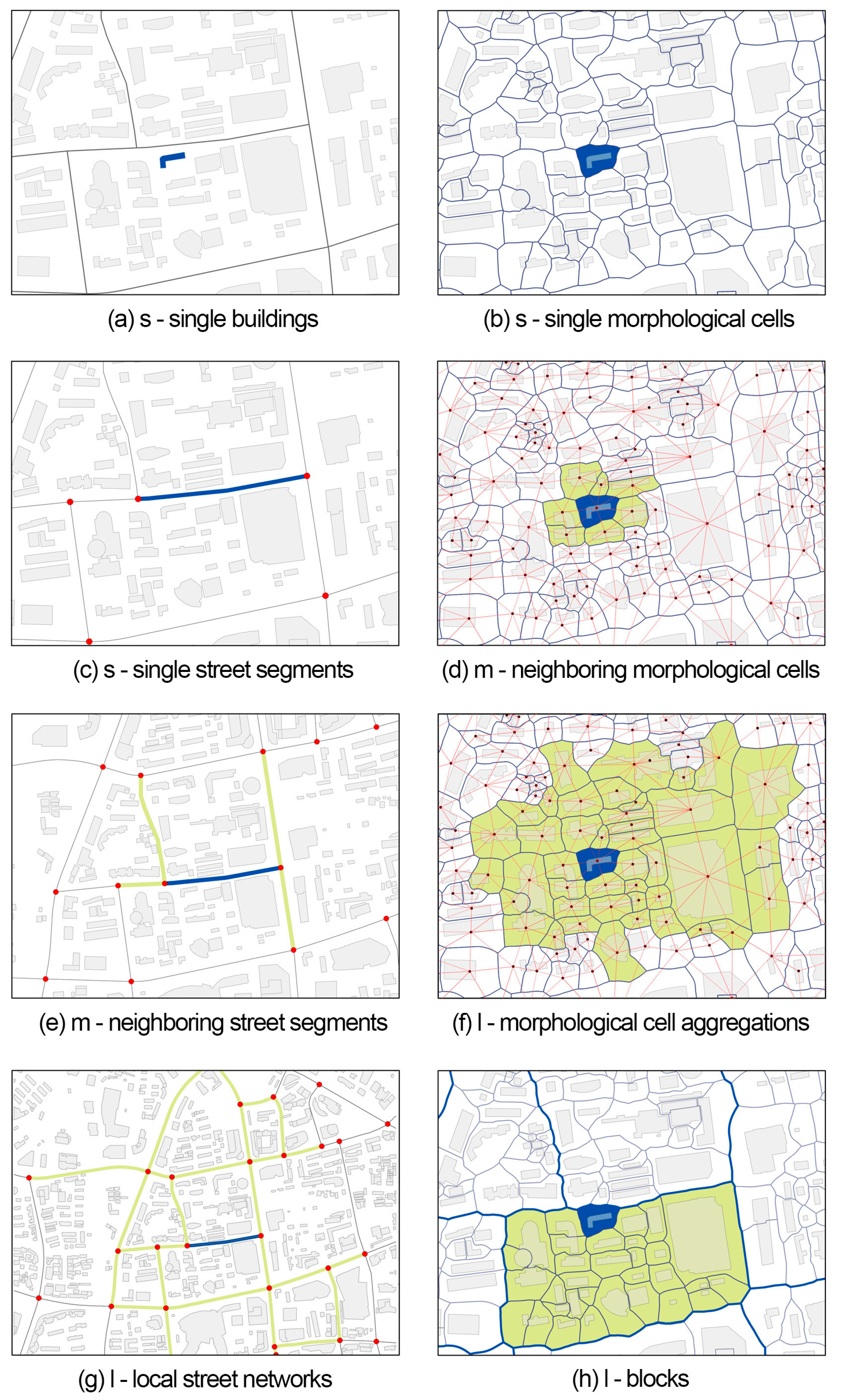
In compiling spatial form indicators, priority should be given to retaining the universality of the method, minimizing potential collinearity, and limiting information redundancy. Following Fleischmann et al. [30], we propose a measurement framework encompassing six key dimensions: dimension (d), shape (s), distribution (t), intensity (i), connectivity (c), and diversity (v). These dimensions are applied to quantify morphological and associated landscape elements, including buildings (b), MCs (c), street segments (s), blocks (k), green vegetation/park green spaces (g), water bodies (w), sky openness (y), and POIs (i.e., points of interest, p). The measurements operate at three topological scales (Figure 3): small (s), i.e., individual element scale, such as single buildings, single MCs, and single street segments; medium (m), i.e., adjacent element scale, including neighboring MCs and neighboring street segments; large (l), i.e., aggregated morphological structure scale within three orders of contiguity, such as MC aggregations, local street networks, blocks, and, in particular, the global street network. This framework is designed to incorporate as many descriptive features as feasible from existing literature.
More importantly, selecting specific indicators should ensure that the nature of regional form, along with its relevant functions, is captured as comprehensively and accurately as possible. In practice, we identified 48 spatial form indicators for application in the subsequent case study (Table 1). This process combined correlation matrix analysis with redundancy checks, applying a Pearson’s correlation coefficient threshold of 0.8. For instance, the indicator sdbAre refers to a dimension (d) measurement of the building (b) area (Are) at a small scale (s). It should be emphasized that the exact indicators used for the measurement of urban landscape spatial form depend on the data availability within specific contexts. Moreover, rather than prescribing a fixed list, we argue that providing broad guidance on the kind of indicators aimed at identifying the typo-morphological characteristics offers greater practical flexibility and value.

2.3. Case Study and Required Data

2.3.1. Case Study

Wuxi China, a key regional central city situated in the heart of the Yangtze River Delta Plain, is selected as the case study, with its continuously built-up area—spanning 38,731 hm2—defined as the study region. As of early 2025, the permanent resident population of Wuxi’s central urban area was approximately 4.4253 million. Geographically positioned between the Yangtze River to the north and Taihu Lake to the south, and intersected by the Grand Canal, Wuxi benefits from advantageous natural conditions that have historically underpinned its development as a fertile and prosperous region. Recognized as a national historical and cultural city with over 2200 years of urban history, Wuxi bears the enduring imprint of Wu culture and a long-standing tradition of industrial and commercial vitality. In the contemporary era, Wuxi functions as both a national transportation hub and an advanced manufacturing center, embodying the accelerated urbanization trajectory observed in many Chinese cities. Infrastructure-driven expansion and policy initiatives have jointly reshaped its spatial form, resulting in a highly complex urban landscape. Applying the proposed typo-morphological analysis framework to the Wuxi case demonstrates its effectiveness in capturing full-scale urban landscape spatial characteristics and validates its broader applicability in complex urban contexts.

2.3.2. Acquisition and Processing of Fundamental Vector Data

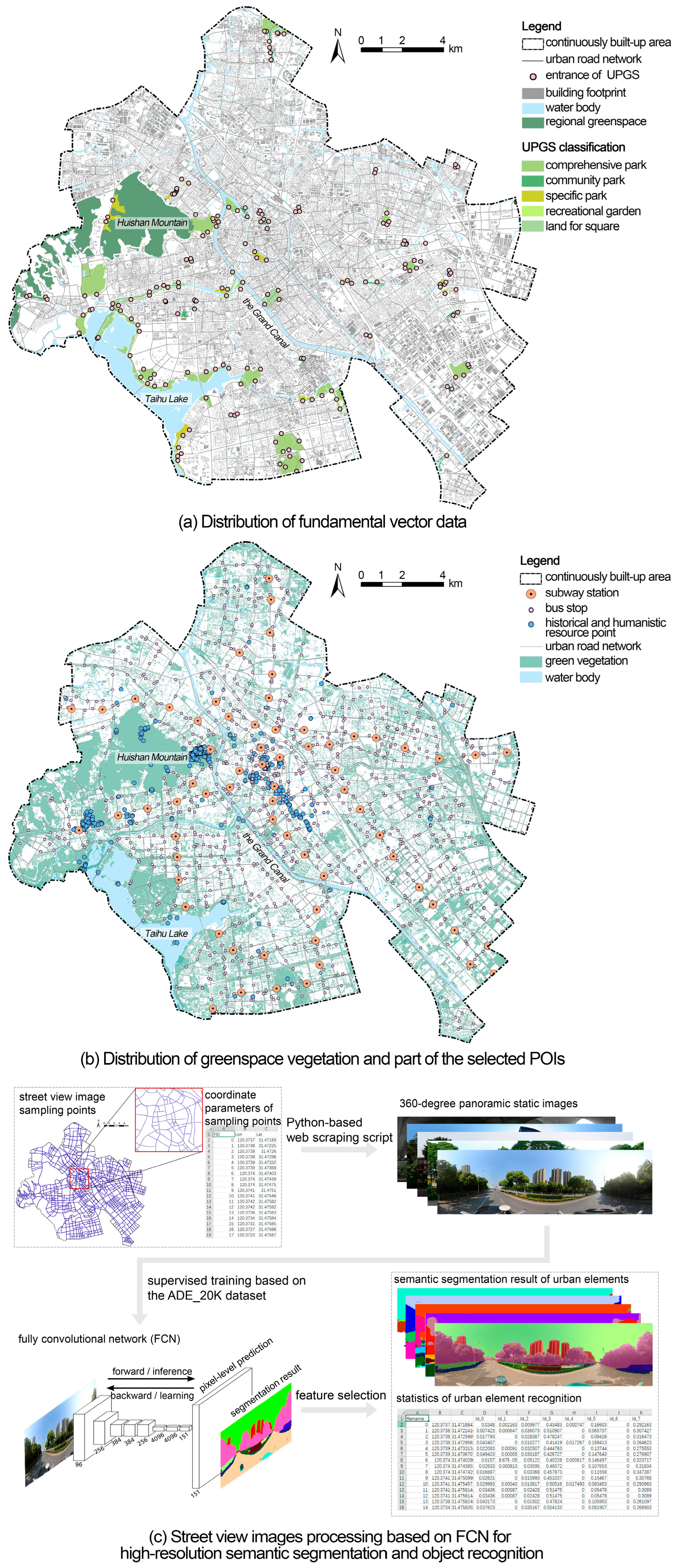
The fundamental vector data utilized in this study comprise urban roads, building footprints, park green spaces, and water bodies, all processed under a unified coordinate system (Figure 4a). The primary road system of Wuxi was selected based on the “Wuxi Urban Master Plan (2001–2020)” and supplemented with open-source data from OpenStreetMap. Necessary adjustments and corrections were made to ensure accuracy. The road network dataset was then constructed within the ArcGIS (version 10.5) platform by converting the “urban road-road intersection” structure into an “edge-node” topological model, thereby establishing the connectivity of the urban road network. The dataset of building footprints was obtained from the Wuxi Municipal Bureau of Natural Resources and Planning. To enhance data completeness, additional building footprint and height information was retrieved using the Baidu Map application programming interface. Buildings with an area smaller than 35 m2 were excluded, as they primarily consist of auxiliary structures. Based on the maps of the “Wuxi Green Space System Plan (2018–2035)”, a total of 60 urban park greenspace polygons were vectorized, covering approximately 13.69 km2. These parks conform to the “National Urban Green Space Classification Standard (CJJ/T85-2017)” [37] and include comprehensive parks (G11), community parks (G12), specific parks (G13), recreational gardens (G14), land for squares with a green coverage ratio of at least 65% (G3). Additionally, the actual entrance locations of all parks were spatially annotated. The distribution of urban water bodies was extracted from Wuxi’s land-use vector dataset, encompassing canals, rivers, lakes, ponds, and reservoirs.

2.3.3. Object-Based Remote Sensing Fine Extraction of Urban Greenspace Information

To achieve high-precision remote sensing extraction of urban greenspace information, this study utilized a GF-2 satellite image of Wuxi, captured during the summer season with a cloud cover of 1%, ensuring high data quality. The GF-2 satellite is a civilian optical remote sensing satellite with sub-meter spatial resolution, equipped with a 1 m panchromatic camera and a 4 m multispectral camera. Following standard remote sensing image preprocessing in ENVI (version 5.3)—including radiometric calibration, atmospheric correction, orthorectification, image fusion, and image cropping—object-based image analysis (OBIA) was conducted using the eCognition (version 9.0.1) platform. This process involved multi-scale segmentation and classification of urban green spaces based on normalized difference vegetation index, green normalized difference vegetation index, and near-infrared reflectance parameters (Figure 4b). OBIA leverages the high spatial resolution of remote sensing imagery by treating image objects as classification units rather than individual pixels. By integrating spectral, textural, shape, and contextual information, OBIA mitigates spectral variability among adjacent pixels, resulting in classification outputs closer to manual visual interpretation. This method significantly enhances classification accuracy while improving computational efficiency by reducing the number of processing units. To validate the reliability of the extracted data, classification accuracy was assessed using a confusion matrix.

2.3.4. Acquisition and Processing of Multi-Source Big Data

128,047 POIs were obtained through the Gaode Map application programming interface and categorized into 14 primary sectors relevant to this study. The distribution of POIs across these categories is as follows: shopping services (31,642), financial and insurance services (1473), catering services (22,782), medical and healthcare services (4079), life services (22,422), accommodation services (2218), companies and enterprises (13,657), commercial residences (3189), science, education, and cultural services (4731), transportation facilities (9697), government institutions and social organizations (5094), tourist attractions (1220), automobile services (2499), and sports and leisure services (3344). Each POI dataset comprises real geospatial point data, including latitude, longitude, and address information, along with attributes such as name and category. Additionally, 67 subway stations and 1167 bus stops were extracted separately from the category of transportation facilities. Meanwhile, subcategories such as natural landmarks, memorials, tourist sites, and temples were manually filtered and consolidated into a dataset of 541 historical and humanistic resource points (Figure 4b).
Street view images provide extensive coverage, high spatial density, and detailed visual representation, making them particularly effective for capturing the human-scale perception of the urban built environment. The rich visual information and objective features embedded in street view images offer a realistic depiction of urban landscapes. Leveraging Baidu Street View’s high-resolution imagery and open accessibility, we systematically sampled along the urban road network at 50 m intervals. A Python-based web scraping script was used to collect 360-degree panoramic static images. Following data cleaning, 25,083 valid images were retained, ensuring the full coverage of the study area. To extract detailed morphometric information, the images were processed using a fully convolutional network for high-resolution semantic segmentation and object recognition. Based on the ADE20K dataset [38], 12 key urban elements were identified for spatial form measurement (Figure 4c), including buildings (Id_2, 26, 49, 80), roads (Id_4, 7), sidewalks (Id_12, 53), sky (Id_3), trees (Id_5, 73), shrubs and grasslands (Id_10, 18, 30), ground surfaces (Id_14, 92, 95), mountains (Id_17, 69), transportation infrastructure (Id_33, 88, 137), billboards (Id_44, 145), walls (Id_1), and bridges (Id_62).

3. Results

3.1. Typologies of Urban Landscape Spatial Characteristics

All 48 spatial form indicators were measured and associated with each MC, yielding 192 tendency-based proxy variables of measurement as input for the cluster analysis.
In addition, the number of components was set to an integer range of 2 to 40 with an interval of 4, with 5 random initializations to mitigate local optima, a full covariance matrix specified as the covariance type, and a maximum of 200 iterations for the expectation–maximization algorithm to ensure sufficient convergence. Under these conditions, the GMM was executed, and model performance was evaluated by examining the BIC results across 3 runs for each number of clusters, rather than relying on the incidental outcome of a single random initialization.
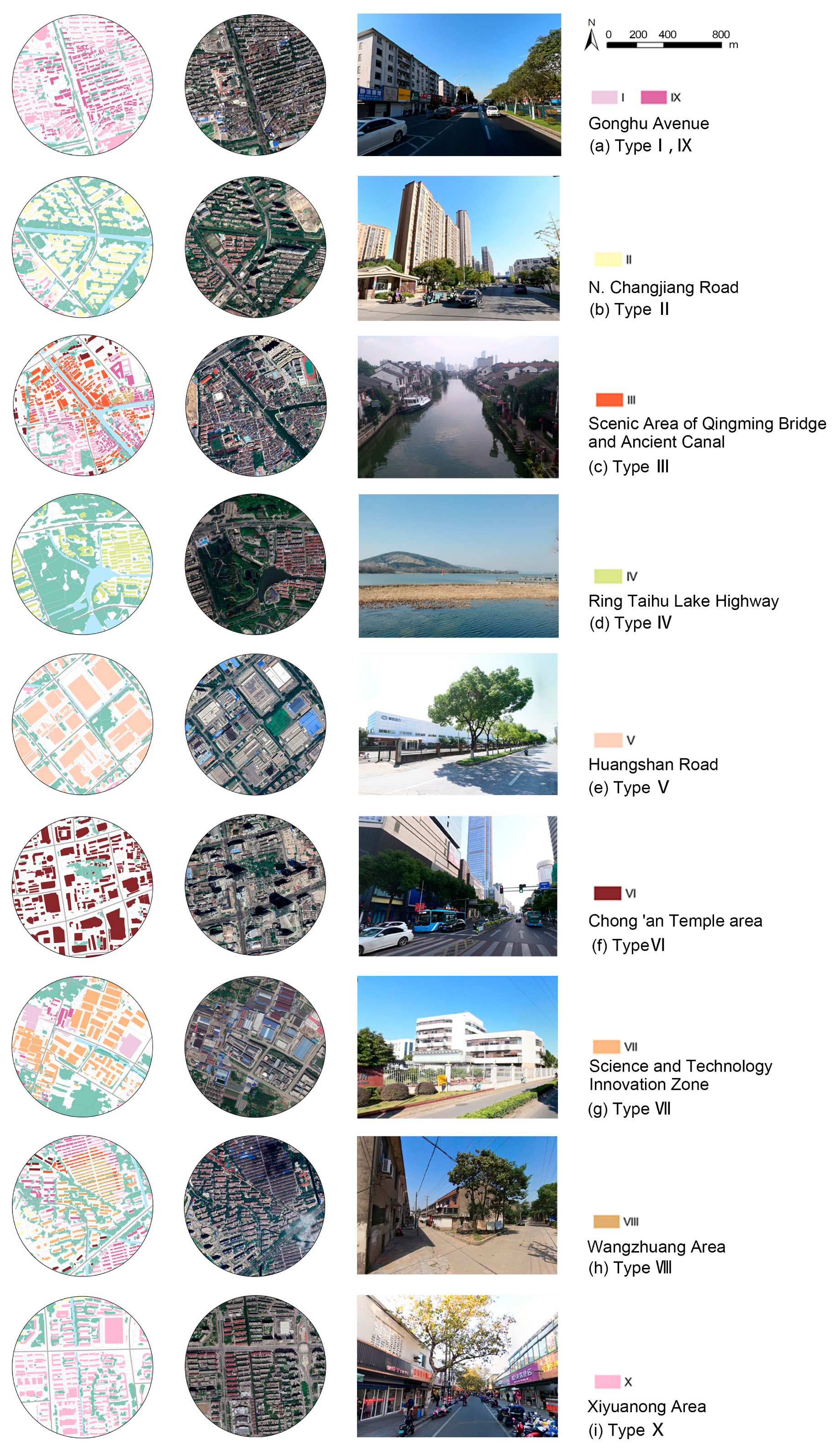
As shown in Figure 5, the selection of 10 clusters was determined by analyzing variations in the BIC value for the corresponding model components, with the shaded area representing the 95% confidence interval. Specifically, the BIC value decreased sharply as the number of clusters increased from 2 to 10, indicating significant improvements in model fit. Within the range of 10 to 14 clusters, the rate of decrease in BIC value slowed markedly, signifying the onset of the “elbow” or plateau region. Beyond 14 clusters, additional clusters resulted in a relatively stable BIC value but introduced unnecessary model complexity. To facilitate the interpretability of the results, the most parsimonious solution within this plateau—represented by 10 clusters—was selected. Moreover, the narrow confidence interval around this solution further indicates robust and stable clustering outcomes, demonstrating minimal sensitivity to random initializations. The actual number of clusters is primarily dictated by the heterogeneity of urban landscape spatial characteristics rather than the overall size of the city. The resulting mapping is depicted in Figure 5, where the geometries define the spatial extent of TMZs generated by clustering, with color coding representing distinct urban landscape types. Furthermore, overlaying the clustering results onto individual building footprints and incorporating a variety of representative sample scenes (Figure 6 presents the selected samples) demonstrates that areas within the same type effectively exhibit a higher degree of similarity in urban texture and functional composition.
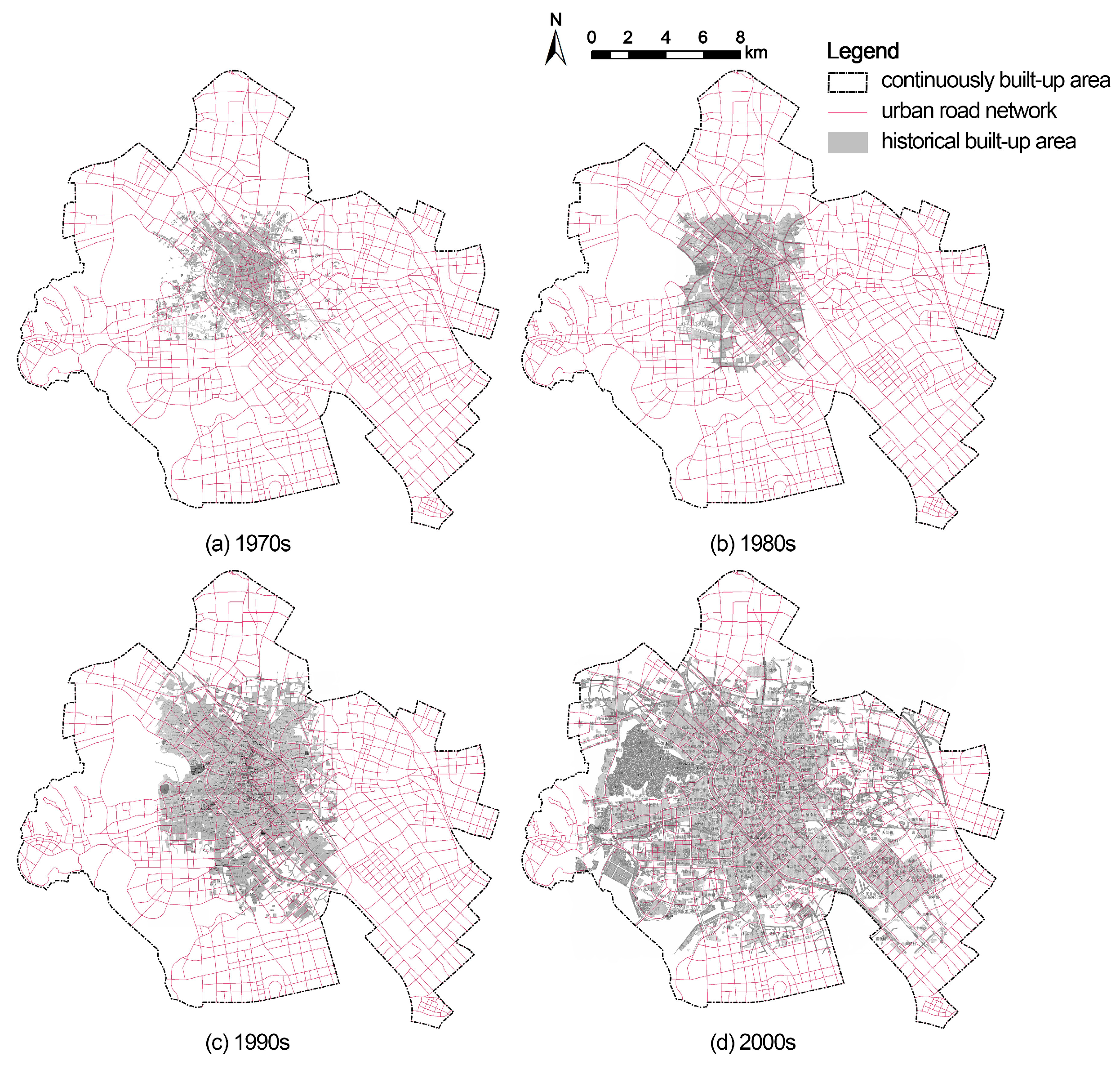
A visual inspection of the identified TMZs reveals clear directional tendencies and concentric gradient patterns in their geographic distribution. When contextualized within Wuxi’s historical urban development, distinct spatial imprints emerge. Since the 1980s, urban expansion has been primarily driven by continuous improvements in transportation infrastructure, facilitating outward growth beyond the historic core. This process accelerated during the urban peak development phase, particularly through three consecutive three-year action plans initiated in 2002, which led to large-scale and systematic urban construction. To a significant extent, the identified clusters reflect these temporally structured spatial patterns. As shown in Figure 5 and Figure 7, the central zone of Type VI closely corresponds to Wuxi’s historic urban core, which remained the dominant locus of continuous urban development up to the 1970s. The planned expansion toward Taihu Lake in the 1980s is primarily reflected in the spatial extent of Type III. The accelerated urbanization of the 1990s and early 2000s is predominantly represented by Types I, IX, and X. Since the mid-2000s, Types II and V have formed increasingly contiguous patches along the urban periphery, while Types VII and VIII have generally emerged at a more recent stage. Notably, Type IV has retained a clearly defined and intact northern boundary, while its eastern margin has shown signs of progressive fragmentation since the 2000s.
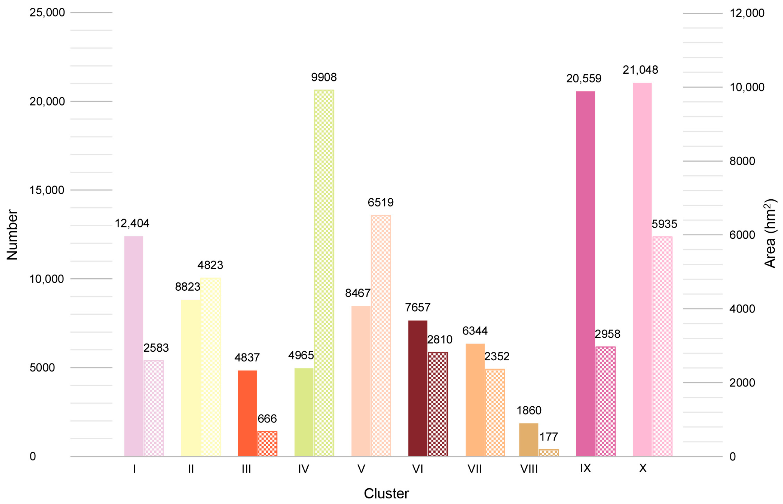
Furthermore, the number and area distribution of MCs across different urban landscape types exhibit substantial variation, as illustrated in Figure 8. The most prevalent types (IX and X) comprise a total of 41,607 MCs, representing approximately 43% of all observations (96,964). However, these types collectively cover only 19% of the study area, indicating that their MCs are generally finer in scale. Type I exhibits a similar characteristic, with an average MC area of just 0.21 hm2. In contrast, Types IV and V, which are primarily distributed in the western part of the city—adjacent to Taihu Lake and Huishan Mountain—as well as in the eastern suburbs, occupy approximately 42% of the total area (nearly 16,427 hm2) despite constituting less than 14% of all MCs. Additionally, a few outlier clusters account for less than 2% of all observations. For instance, Type VIII covers only 177 hm2.

3.2. Hierarchical Relationships Among Urban Landscape Types

The centroid values of each cluster, computed as the mean values of the tendency-based proxy variables of 48 spatial form measurements within the clustered MCs, serve as taxonomic characters in the connection matrix calculation of Ward’s hierarchical clustering to reveal the relationships among urban landscape types based on morphological similarity (Figure 9). In the dendrogram, the vertical axis denotes the cophenetic distance of the identified clusters, and bifurcations represent nested levels of landscape differentiation. A lower connecting link between two clusters indicates a lower merging cost and a higher degree of characteristic similarity, and vice versa.
The dendrogram of Wuxi’s urban landscape spatial characteristics delineates 10 clusters, with two major bifurcations indicating distinct higher-order groupings at different levels of cophenetic distance. One group encompasses Types I, VIII, and IX, which are morphologically characterized by small, fragmented patches dispersed throughout the study area. The other group comprises the remaining types, primarily forming large, contiguous spatial zones. Notably, the dendrogram reveals three relatively independent branches corresponding to distinct urban landscape types: blue-green resource-rich areas (Type IV), industrial parks (Type V), and mixed residential zones comprising urban villages and resettlement housing (Type VIII). Additionally, a lower-order bifurcation within the main branch differentiates regular-strip blocks (Type IX) and their adjacent peripheral areas (Type I). Moreover, the dendrogram identifies another pair of morphologically similar types. For instance, Type VI captures the cores of urban development represented by the old town, while its counterpart, Type X, reflects rapid developments mainly based on residence that have emerged in a radial pattern since the late 20th century.

4. Discussion

4.1. Key Spatial Form Tendency Variables Influencing Global Typological Decisions

Rather than serving as a simple mixture of spatial form indicators, the identified clusters represent distinct spatial typologies that encapsulate distributional morphological characteristics. To further elucidate the underlying mechanisms of TMZ generation, we employed the classification and regression tree (CART) machine-learning algorithm to assess the relative importance of individual spatial form conditions driving typological decisions while simultaneously achieving dimensionality reduction. Given the presence of continuous attributes in the medium-to-large dataset used in this study, the CART algorithm, supported by pruning techniques, offers significant advantages in controlling tree complexity and mitigating overfitting. Furthermore, its construction principle—binary recursive partitioning guided by impurity minimization ensures interpretability, computational efficiency, and robustness.
In the dataset of MCs corresponding to each urban landscape type, 70% of the samples were randomly selected for training and constructing decision tree, while the remaining 30% constituted the test set. The Gini coefficient was employed as the criterion for evaluating the quality of tree splits, with the optimal splitting attribute at each node (i.e., a specific tendency-based proxy variable of spatial form measurements and its corresponding threshold) determined to minimize data impurity. To comprehensively assess model performance, the optimal pre-pruning hyperparameters were configured as follows: a minimum sample size of 100 for internal node splitting, a minimum sample size of 50 for leaf nodes, and a maximum tree depth of 10. Under this configuration, the model achieved an accuracy of approximately 0.85.
The final normalized importance scores of spatial form tendency variables in the predictive model were derived to quantify their relative contributions. Table 2 presents the top 14, whose cumulative importance score, approaching 0.80, demonstrates their strong explanatory power in the overall typology. Notably, in the context of a high-density built environment, such as Wuxi, the results underscore the dominant influence of density-related variables across multiple topological scales. These include the following: service density covered by a street segment (sicDen_theilID3, sicDen_rangeIQ3, sicDen_meanIQ3), density of neighboring cells (micDen_meanIQ3), density of MCs within a block (licDen_meanIQ3), service density covered by a MC aggregation (likDen_meanIQ3). Several variables, such as lcbRea_theilID3, lcbBet_meanIQ3, and lcbClo_rangeIQ3, associated with urban network centrality of reach, betweenness, and closeness, highlight the crucial role of the potential spatial structural relationship and its movement affordances. Additionally, other highly ranked variables, such as reached historical and humanistic resource POI number by a MC aggregation (ltpRea_simpson), proximity of water bodies within a local street network (ltwPro_rangeIQ3), height of a building (sdbHei_simpson), windingness of a street segment (sssWin_theilID3), average width of a street segment (sdsAvW_theilID3), the strong predictive performance of these variables in typological decision is consistent with their correspondence to spatial attributes that are most readily perceived and cognitively processed in individuals’ day-to-day interactions with the urban environment. In Table 2, the thresholds of the selected spatial form tendency variables across different urban landscape types are expressed using the interdecile range. This approach minimizes the impact of outliers and extreme values while capturing the general patterns of corresponding urban landscape spatial characteristics to a certain extent. It is important to note that these key spatial form tendency variables are specific to make a global distinction among the TMZs in this case study. The precise identification feature conditions of each urban landscape type should be extracted based on a detailed decision process.

4.2. Key Spatial Form Conditions and Feature Points for Specific Typological Decisions

Unlike “black-box” models such as neural networks, CART decision trees generate a set of interpretable rules that elucidate the underlying logic of data classification while demonstrating strong predictive performance on new instances. Furthermore, by integrating the tools of Graphviz and Dtreeviz, the decision process can be effectively visualized, offering a clearer representation of the spatial form conditions and corresponding feature points that truly influence different urban landscape types.
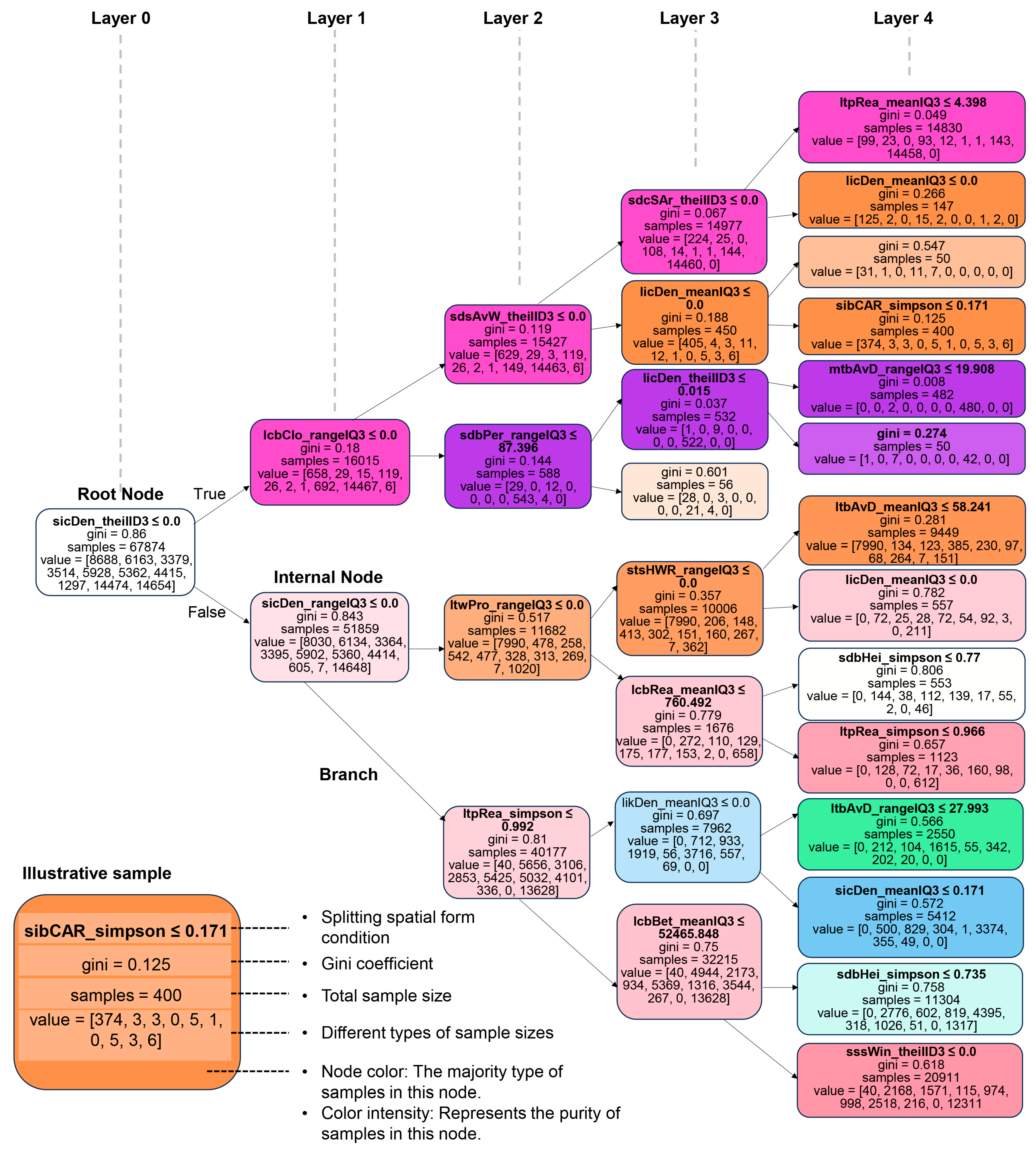
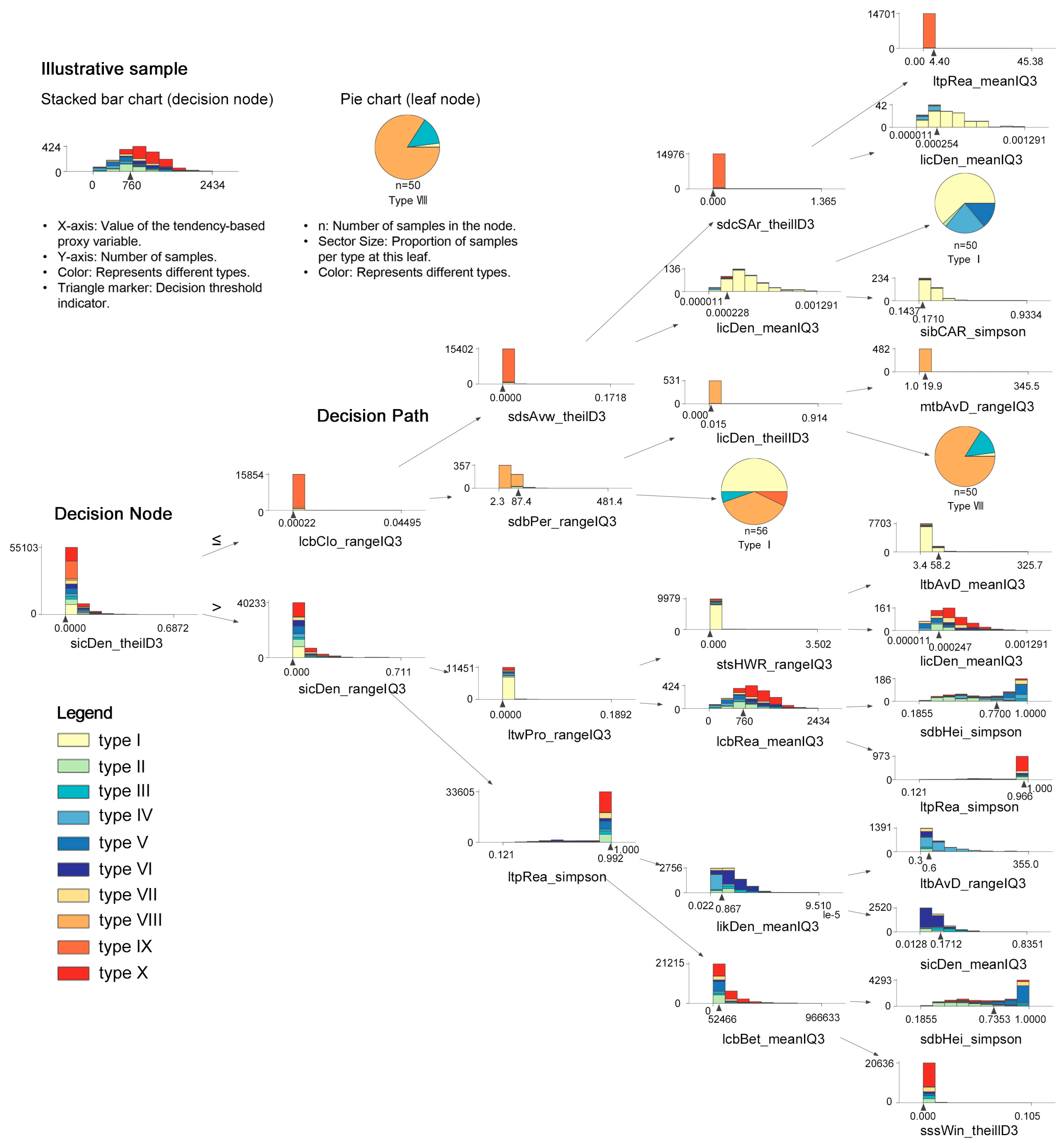
Given the extensive structure of the decision tree, each node represents the splitting spatial form conditions, the Gini coefficient, the total sample size, and the distribution of samples across target types. To enhance clarity in decision details, Figure 10 presents an illustrative structure diagram generated via Graphviz, depicting layers 0–4 as a schematic representation, while the full decision tree can be reconstructed using the corresponding script file provided in Supplementary File S2. Additionally, Dtreeviz is employed to generate stacked histograms at each node, incorporating annotations of extreme values and split thresholds for specific spatial form conditions (Figure 11). This approach offers a more intuitive visualization of hierarchical and purity changes in data distribution. Furthermore, pie charts illustrate the proportion of dominant types within the leaf nodes.
Based on the evidence presented in Figure 10 and Figure 11, a deeper interpretation of Table 3 and Table 4 was concluded. Taking Type I as an example, Table 3 presents its primary classification path as derived from the decision tree. The first-layer split is based on the condition “sicDen_rangeIQ3≤0”, followed by nine successive feature-based splits, ultimately reaching the leaf node dominated by Type I at the tenth layer. This leaf node contains a total of 8185 samples, with Type I accounting for approximately 95%, and a Gini coefficient of 0.096, indicating high data purity. Notably, after the first three splits, the cumulative reduction in data impurity—measured by the Gini coefficient—reaches 0.562 (i.e., 0.326 + 0.16 + 0.076). At this stage, the number of Type I samples stabilizes at 7990, covering 91.97% of its total sample count (8688), while simultaneously eliminating 42,370 samples from other types. Given this high classification efficiency, service density covered by a street segment (sicDen_rangeIQ3), proximity of water bodies within a local street network (ltwPro_rangeIQ3), and height-to-width ratio of a street segment (stsHWR_rangeIQ3), along with their corresponding threshold values, can be identified as the dominant spatial form conditions for distinguishing Type I. Furthermore, an analysis of the cost–benefit ratio—defined as the ratio of target sample loss to the number of excluded non-target samples at each selection of splitting attributes—reveals that while closeness (centrality) within a global street network (lcbClo_rangeIQ3), proximity of water bodies within a local street network (sdsLen_rangeIQ3), and height to width ratio of a street segment (svsDiv_theilID3) contribute less to Gini gain, they significantly enhance impurity reduction by effectively eliminating samples from other types. As such, they can be regarded as auxiliary spatial form conditions for Type I decision. By applying this approach, we infer the key spatial form conditions that play a decisive role in distinguishing different urban landscape types, along with their underlying feature points, as summarized in Table 4.

4.3. Advantages, Prospects, and Limitations of the Research Approach

Amidst the worldwide trend toward high-density urbanization, many cities are increasingly characterized by large spatial scales, mixed land uses, and frequent renewal cycles. As noted in the Section 1, a long-standing challenge of morphological analysis lies in its limited practical utility when confronted with massive urban datasets and the demands of fine-grained governance. This underscores the need for the digital transformation of urban landscape characterization through intelligent, data-driven approaches.
Indeed, recent years have seen the emergence of several related representative models. For instance, Pont and Haupt systematically developed an urban spatial typo-morphological analysis method based on the measurement of materialized density [39]. They constructed a three-dimensional diagrammatic model—Spacematrix—with multivariable density and proposed it as a morphological descriptive tool for quantitative urban design. This tool aids planners and designers in evaluating existing spatial capacity while simultaneously setting appropriate conditions for future spatial development [40]. Similarly, leveraging the quantitative effectiveness of Spacematrix, Space Syntax, and the Mixed-Use Index, Ye et al. synthesized an analytical framework for urban spatial morphological characteristics in their evidence-based investigation into the spatial form of urban vitality [41]. They further operationalized this framework by creating VitalVizor, a visual analytical system tool [41,42]. However, prevailing methods generally exhibit limitations in their capacity to synthesize morphological dimensions, integrate morphological and associated landscape elements, and operate across diverse environmental scales. These constraints are primarily attributable to the challenges in acquiring accurate cadastral plot data, which have conventionally served as the fundamental spatial units for morphological quantification. By contrast, MCs generated from building footprints (and street networks)—data that are themselves available from multiple sources—offer a versatile medium for hosting and linking more detailed, extensive, and valuable urban spatial information. It demonstrates significant cost advantages.
Our approach, combining GMM with a decision tree (i.e., CART), effectively decouples the exploration and explanation phases, which offers several advantages. (1) Handling complexity: Unlike methods reliant on linear assumptions, the proposed framework exhibits a superior capacity for handling complexity. It is particularly adept at capturing non-linear relationships and complex interaction effects among variables, making it exceptionally suited for modeling the intricate and heterogeneous nature of urban data. This capability enables a more flexible and assumption-lean workflow that seamlessly integrates classification, interpretation, and prediction. (2) Unbiased discovery: To ensure an objective and data-driven exploration of urban landscape types, GMM was employed for the clustering phase. Unlike supervised methods, such as discriminant analysis, which require pre-labeled training data, GMM operates without prior guidance to identify latent structures, grouping entities based on morphological similarity and allowing natural groupings to emerge organically from the feature set. This approach circumvents the subjectivity and potential biases inherent in researcher-defined taxonomies, thereby yielding a more robust and authentic representation of the intrinsic diversity of urban landscape spatial characteristics. (3) Enhanced interpretability: The subsequent application of the CART model provides a transparent, flowchart-like set of decision rules that elucidate the rationale behind cluster assignments. It is contended that these rule-based explanations furnish urban planners and policy-makers with a more intuitive and directly actionable framework than the outputs of linear equation-based, probabilistic classification models. Each condition within the rule set derived from our analysis represents an interpretable, physically meaningful threshold within the professional domain. These thresholds can be directly translated into specific, quantifiable planning targets and design criteria, while also providing a clear hierarchy of variable importance.
Furthermore, the proposed research approach can be extended to facilitate time-series change analysis, as well as to routine domains such as urban physical examination, planning implementation monitoring, and urban renewal potential evaluation. Looking ahead, it opens opportunities for novel modes of human–computer collaboration in planning practice. By establishing an intelligent, self-adaptive rule-based learning system, it can significantly enhance its generalization capability for application across diverse urban contexts, thereby providing robust support for fine-grained urban governance. For instance, in August 2025, the Chinese government unveiled a guideline aimed at promoting high-quality urban development. This national-level directive explicitly states that “China’s urbanization is shifting from a phase of rapid expansion to that of stable development. Urban growth is transitioning from large-scale incremental expansion to a stage focused on improving the quality and efficiency of existing capacity”. In this context, developing consistent frameworks to characterize cities and track their evolution has never been more important. Regarding theoretical research, this framework can be employed to conduct interdisciplinary studies that link the spatial characteristics of urban landscapes with their ecosystem service value, environmental performance, or economic productivity, thus contributing to the sustainable development of future cities.
Relevant methodological approaches have been preliminarily attempted in several cities distributed across different global regions (e.g., Barcelona, Europe; Houston, North America; Medellín, South America; Dar es Salaam, Africa; Singapore, Southeast Asia) [27]. The diverse manifestations of these similar concepts under different contexts can effectively facilitate cross-sectional comparisons among various city types and may even foster the development of a more comprehensive urban typological system. For instance, a macro-scale comparison reveals certain similarities in the distribution of urban landscape heterogeneity between Wuxi, China, and Boston, USA. Both cities exhibit clear directional tendencies and concentric gradient patterns. However, the typological patches in Wuxi are more fragmented and exhibit weaker spatial continuity. It must be acknowledged that the proposed framework is particularly well-suited to complex built environments in medium- and large-scale cities, where urban data are abundant and morphological differentiation across types is more pronounced. In contrast, its applicability may be limited in smaller towns, suburban areas, or scenic districts, which often possess a more integral morphological structure. Finally, we recommend that, with ongoing technological and societal advances in data generation, additional information—such as on urban (green) open spaces and public perceptions—should be integrated into this framework. This will further enrich the interpretation of urban landscape spatial morphological characteristics and align it more closely with lived experiential reality.

5. Conclusions

Contemporary urban landscape planning, development, and management increasingly operate at the scale of holistic spatial form, thereby necessitating new theoretical frameworks and analytical techniques capable of effectively capturing the inherent spatial characteristics of urban landscapes. This study introduces a comprehensive morphometric framework designed to objectively and generatively delineate urban spatial patterns based on typo-morphology. By attaching 48 constructed spatial form indicators to MCs, as the urban morphometric spatial units, the framework enables a fine-grained and computationally efficient representation of complex urban environments. The metrical information is systematically grouped into coherent TMZs through unsupervised clustering.
The application to Wuxi City demonstrates that the landscape spatial characteristics reflected in the typological mapping outputs can trace temporal urban expansion and stratify landscape structures, while also facilitating bottom-up interpretability. More importantly, through a universal conceptual medium of spatial form, these characteristics can feed back directly into the creative organization of landscape planning and design. This study thus highlights the potential of morphometric-based typologization of spatial characteristics as a standardized, scalable tool for environmental impact assessments, urban landscape governance, and sustainable spatial planning.

Supplementary Materials

The following supporting information can be downloaded at https://www.mdpi.com/article/10.3390/land14091854/s1, File S1: Formulas of 48 spatial form indicators; File S2: The script file of the full decision tree.

Author Contributions

Conceptualization, Y.F., H.Z. and Y.C.; methodology, Y.F., H.Z. and Y.C.; software, Y.F.; validation, H.Z., T.Z. and B.F.; formal analysis, Y.F. and H.Z.; investigation, Y.F., T.Z. and B.F.; resources, H.Z. and Y.C.; data curation, Y.F. and H.Z.; writing—original draft preparation, Y.F. and H.Z.; writing—review and editing, Y.F. and H.Z.; visualization, Y.F., H.Z. and T.Z.; supervision, Y.C.; funding acquisition, Y.C. All authors have read and agreed to the published version of the manuscript.

Funding

This research was funded by the National Natural Science Foundation of China, grant number 51838003.

Data Availability Statement

The data presented in this study are available from the corresponding author on reasonable request.

Conflicts of Interest

The authors declare no conflicts of interest. The funders had no role in the design of the study; in the collection, analyses, or interpretation of data; in the writing of the manuscript; or in the decision to publish the results.

Abbreviations

The following abbreviations are used in this manuscript:
MC(s)Morphological cell(s)
TMZ(s)Typo-morphological zone(s)
GMMGaussian mixture model
BICBayesian information criterion
OBIAObject-based image analysis
POI(s)Point(s) of interest
CARTClassification and regression tree

References

  1. Batty, M. A research programme for urban morphology. Environ. Plan. B Plan. Des. 1999, 26, 475–476. [Google Scholar] [CrossRef]
  2. Andersson, E.; Barthel, S.; Borgström, S.; Colding, J.; Elmqvist, T.; Folke, C.; Gren, Å. Reconnecting cities to the biosphere: Stewardship of green infrastructure and urban ecosystem services. Ambio 2014, 43, 445–453. [Google Scholar] [CrossRef]
  3. Marcus, L.; Pont, M.B.; Barthel, S. Towards a socio-ecological spatial morphology: Integrating elements of urban morphology and landscape ecology. Urban Morphol. 2019, 23, 115–124. [Google Scholar] [CrossRef]
  4. Kropf, K. An Enquiry into the Definition of Built Form in Urban Morphology. Ph.D. Thesis, University of Birmingham, Birmingham, UK, 1993. [Google Scholar]
  5. Osmond, P. The urban structural unit: Towards a descriptive framework to support urban analysis and planning. Urban Morphol. 2010, 14, 5–20. [Google Scholar] [CrossRef]
  6. Pauleit, S.; Duhme, F. Assessing the metabolism of urban systems for urban planning. In Urban Ecology; Breuste, J., Feldmann, H., Uhlmann, O., Eds.; Springer: Berlin/Heidelberg, Germany, 1998; pp. 65–69. [Google Scholar] [CrossRef]
  7. Wickop, E. Environmental quality targets for urban structural units in Leipzig with a view to sustainable urban development. In Urban Ecology; Breuste, J., Feldmann, H., Uhlmann, O., Eds.; Springer: Berlin/Heidelberg, Germany, 1998; pp. 49–54. [Google Scholar] [CrossRef]
  8. Scheer, B.C. Towards a minimalist definition of the plot. Urban Morphol. 2018, 22, 162–163. [Google Scholar]
  9. Forman, R.T. Land Mosaics: The Ecology of Landscapes and Regions, 1st ed.; Cambridge University Press: New York, NY, USA, 1995. [Google Scholar] [CrossRef]
  10. Löfvenhaft, K.; Björn, C.; Ihse, M. Biotope patterns in urban areas: A conceptual model integrating biodiversity issues in spatial planning. Landsc. Urban Plan. 2002, 58, 223–240. [Google Scholar] [CrossRef]
  11. Ståhle, A. Sociotope mapping: Exploring public open space and its multiple use values in urban and landscape planning practice. Nord. J. Archit. Res. 2006, 19, 59–71. [Google Scholar]
  12. Ståhle, A. Urban planning for a quality dense green structure, Stockholm sociotop map and park programme. In COST Action C1—Green Structure and Urban Planning—Final Report; Werquin, A.C., Duhem, B., Lindholm, G., Oppermann, B., Pauleit, S., Tjallingii, S., Eds.; Office for Official Publications of the European Communities: Luxembourg, 2005; pp. 287–293. [Google Scholar]
  13. Ye, Y.; Huang, R.; Zhang, L.Z. Quantitative urban morphology: Emergence, conceptualization and urban design’s response. Time Archit. 2021, 34–43. [Google Scholar] [CrossRef]
  14. Samuels, I. ISUF task force on research and practice in urban morphology: Interim report. Urban Morphol. 2013, 17, 40–43. [Google Scholar]
  15. Arribas-Bel, D. Accidental, open and everywhere: Emerging data sources for the understanding of cities. Appl. Geogr. 2014, 49, 45–53. [Google Scholar] [CrossRef]
  16. Fleischmann, M.; Feliciotti, A.; Kerr, W. Evolution of urban patterns: Urban morphology as an open reproducible data science. Geogr. Anal. 2022, 54, 536–558. [Google Scholar] [CrossRef]
  17. Glaeser, E.L.; Kominers, S.D.; Luca, M.; Naik, N. Big data and big cities: The promises and limitations of improved measures of urban life. Econ. Inq. 2018, 56, 114–137. [Google Scholar] [CrossRef]
  18. Wei, L.; Luo, Y.; Wang, M.; Cai, Y.; Su, S.; Li, B.; Ji, H. Multiscale identification of urban functional polycentricity for planning implications: An integrated approach using geo-big transport data and complex network modeling. Habitat Int. 2020, 97, 102134. [Google Scholar] [CrossRef]
  19. Araldi, A.; Fusco, G. From the street to the metropolitan region: Pedestrian perspective in urban fabric analysis. Environ. Plan. B Urban Anal. City Sci. 2019, 46, 1243–1263. [Google Scholar] [CrossRef]
  20. Bobkova, E.; Berghauser Pont, M.; Marcus, L. Towards analytical typologies of plot systems: Quantitative profile of five European cities. Environ. Plan. B Urban Anal. City Sci. 2021, 48, 604–620. [Google Scholar] [CrossRef]
  21. Dibble, J.; Prelorendjos, A.; Romice, O.; Zanella, M.; Strano, E.; Pagel, M.; Porta, S. On the origin of spaces: Morphometric foundations of urban form evolution. Environ. Plan. B Urban Anal. City Sci. 2019, 46, 707–730. [Google Scholar] [CrossRef]
  22. Gil, J.; Beirão, J.N.; Montenegro, N.; Duarte, J.P. On the discovery of urban typologies: Data mining the many dimensions of urban form. Urban Morphol. 2012, 16, 27–40. [Google Scholar] [CrossRef]
  23. Wang, J.G. Digital urban design based on human-computer interaction: Discussion on the fourth generation of urban design. Urban Plan. Int. 2018, 33, 1–6. [Google Scholar] [CrossRef]
  24. Fleischmann, M.; Feliciotti, A.; Romice, O.; Porta, S. Morphological tessellation as a way of partitioning space: Improving consistency in urban morphology at the plot scale. Comput. Environ. Urban. Syst. 2020, 80, 101441. [Google Scholar] [CrossRef]
  25. Hamaina, R.; Leduc, T.; Moreau, G. Towards urban fabrics characterization based on buildings footprints. In Bridging the Geographic Information Science; Gensel, J., Josselin, D., Vandenbroucke, D., Eds.; Springer: Berlin/Heidelberg, Germany, 2012; pp. 327–346. [Google Scholar] [CrossRef]
  26. Usui, H.; Asami, Y. Estimation of mean lot depth and its accuracy. J. City Plan. Inst. Jpn. 2013, 48, 357–362. [Google Scholar] [CrossRef]
  27. Arribas-Bel, D.; Fleischmann, M. Spatial signatures-understanding (urban) spaces through form and function. Habitat Int. 2022, 128, 102641. [Google Scholar] [CrossRef]
  28. Usui, H.; Asami, Y. Size distribution of urban blocks in the Tokyo Metropolitan Region: Estimation by urban block density and road width on the basis of normative plane tessellation. Int. J. Geogr. Inf. Sci. 2018, 32, 120–139. [Google Scholar] [CrossRef]
  29. Fleischmann, M. Momepy: Urban morphology measuring toolkit. J. Open Source Softw. 2019, 4, 1807. [Google Scholar] [CrossRef]
  30. Fleischmann, M.; Feliciotti, A.; Romice, O.; Porta, S. Methodological foundation of a numerical taxonomy of urban form. Environ. Plan. B Urban Anal. City Sci. 2022, 49, 1283–1299. [Google Scholar] [CrossRef]
  31. Duque, J.C.; Anselin, L.; Rey, S.J. The max-p-regions problem. J. Reg. Sci. 2012, 52, 397–419. [Google Scholar] [CrossRef]
  32. Vermunt, J.K.; Magidson, J. Latent class cluster analysis. In Applied Latent Class Analysis; Hagenaars, J.A., McCutcheon, A.L., Eds.; Cambridge University Press: New York, NY, USA, 2002; pp. 89–106. [Google Scholar] [CrossRef]
  33. Dahl, D.B. Model-based clustering for expression data via a Dirichlet process mixture model. In Bayesian Inference for Gene Expression and Proteomics; Do, K.A., Müller, P., Vannucci, M., Eds.; Cambridge University Press: New York, NY, USA, 2006; pp. 201–218. [Google Scholar] [CrossRef]
  34. Bouveyron, C.; Brunet-Saumard, C. Model-based clustering of high-dimensional data: A review. Comput. Stat. Data Anal. 2014, 71, 52–78. [Google Scholar] [CrossRef]
  35. Schwarz, G. Estimating the dimension of a model. Ann. Stat. 1978, 6, 461–464. [Google Scholar] [CrossRef]
  36. Ward, J.H., Jr. Hierarchical grouping to optimize an objective function. J. Am. Stat. Assoc. 1963, 58, 236–244. [Google Scholar] [CrossRef]
  37. CJJ/T85-2017; National Urban Green Space Classification Standard. China Architecture Publishing & Media Co., Ltd.: Beijing, China, 2017.
  38. Zhou, B.; Zhao, H.; Puig, X.; Fidler, S.; Barriuso, A.; Torralba, A. Scene parsing through ADE20K dataset. In Proceedings of the 2017 IEEE Conference on Computer Vision and Pattern Recognition (CVPR), Honolulu, HI, USA, 21–26 July 2017; IEEE: Piscataway, NJ, USA, 2017; pp. 633–641. [Google Scholar] [CrossRef]
  39. Pont, M.B.; Haupt, P. Spacematrix: Space, Density and Urban Form, Revised ed.; TU Delft OPEN Publishing: Delft, The Netherlands, 2023. [Google Scholar] [CrossRef]
  40. Pont, M.B.; Haupt, P. The Spacemate: Density and the typomorphology of the urban fabric. Nord. J. Archit. Res. 2015, 18, 55–68. [Google Scholar]
  41. Ye, Y.; Nes, A.v.N. Quantitative tools in urban morphology: Combining Space Syntax, Spacematrix and Mixed-Use Index in a GIS framework. Urban Morphol. 2014, 18, 97–118. [Google Scholar] [CrossRef]
  42. Zeng, W.; Ye, Y. VitalVizor: A visual analytics system for studying urban vitality. IEEE Comput. Graph. Appl. 2018, 38, 38–53. [Google Scholar] [CrossRef] [PubMed]
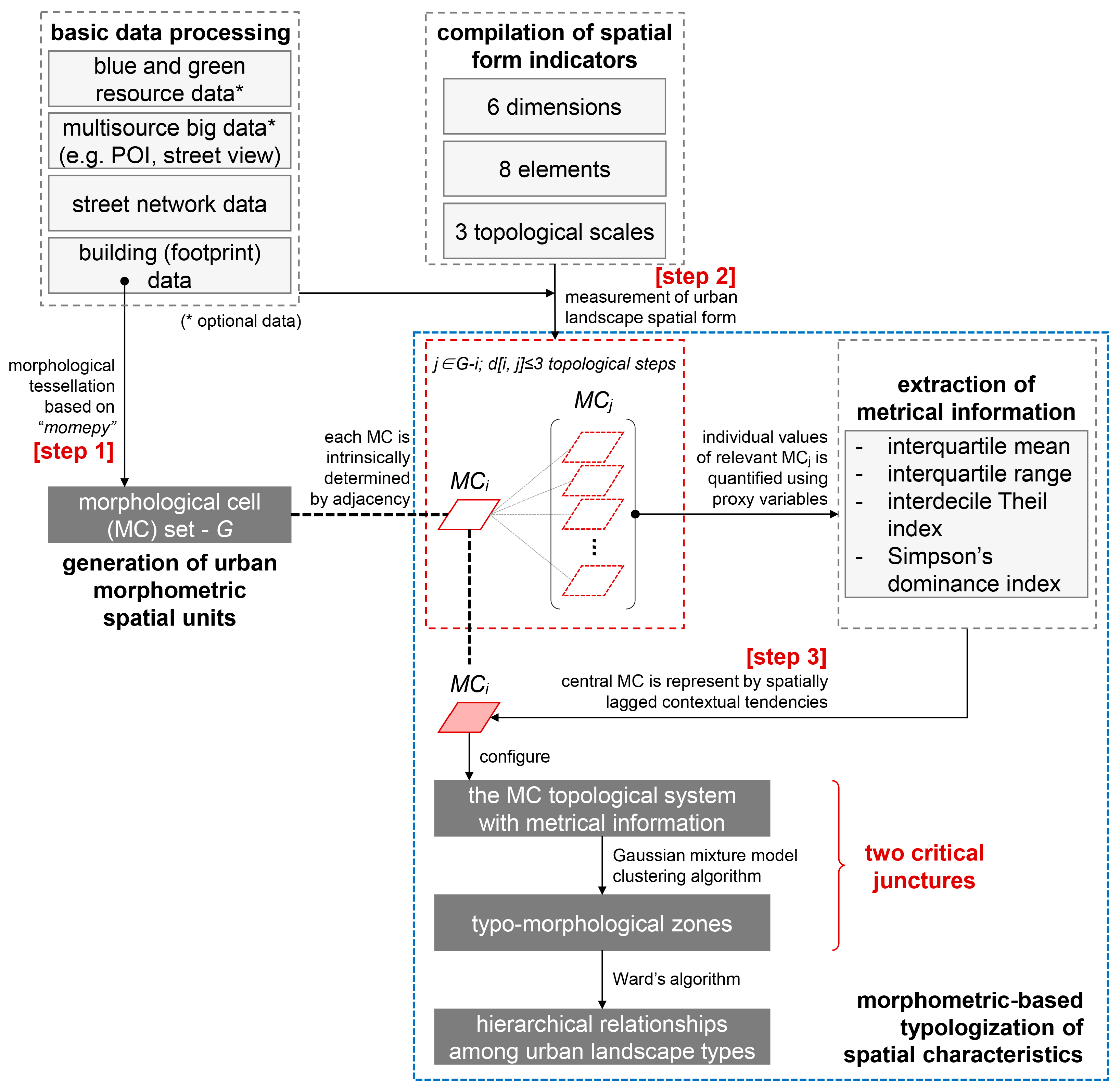
Figure 1. Diagram describing the methodology.
Land 14 01854 g001
Figure 2. The spatially lagged context derived from the topological structure of each given MC, for the tendency quantification of individual values in the area.
Land 14 01854 g002
Figure 3. The measurement environment setting of spatial form based on three topological scales.
Land 14 01854 g003
Figure 4. Processing of data related to the study case (Wuxi City, China).
Land 14 01854 g004
Figure 5. Variations in the BIC value for the corresponding numbers of clusters, with the shaded area representing the 95% confidence interval (right) and the spatial extent of TMZs generated by clustering (left).
Land 14 01854 g005
Figure 6. Typical samples of each urban landscape type are presented using building distribution maps overlaid with clustering results, accompanied by corresponding satellite and street view images. Notably, since Type I frequently appears as a peripheral extension of Type IX, these two types are displayed together to facilitate comparative analysis.
Land 14 01854 g006
Figure 7. The urban expansion of Wuxi aligns closely with the spatial configuration of the identified clusters, highlighting the temporal layering of urban growth and its reflection in TMZs.
Land 14 01854 g007
Figure 8. The number and area distribution of MCs across different urban landscape types.
Land 14 01854 g008
Figure 9. Hierarchical relationships among urban landscape types.
Land 14 01854 g009
Figure 10. Schematic illustration of the decision logic for urban landscape typologies based on spatial form conditions (partial view, layers 0–4 of the decision tree).
Land 14 01854 g010
Figure 11. Visualization of hierarchical variation and data purity in the decision process for urban landscape typologies (partial view, layers 0–4 of the decision tree).
Land 14 01854 g011
Table 1. Spatial form indicators identified based on multi-dimensional cognition of full-scale morphological and associated landscape elements.
No.ScalesDimensionsElementsFeaturesIndicators *
01s–single buildingsdimension (d)buildings (b)AreasdbAre
02s–single buildingsdimension (d)buildings (b)HeightsdbHei
03s–single buildingsdimension (d)buildings (b)PerimetersdbPer
04s–single buildingsdimension (d)buildings (b)VolumesdbVol
05s–single buildingsshape (s)buildings (b)Circular CompactnessssbCCo
06s–single buildingsshape (s)buildings (b)Equivalent Rectangular IndexssbERI
07s–single buildingsshape (s)buildings (b)ElongationssbElo
08s–single buildingsdistribution (t)buildings (b)OrientationstbOri
09s–single MCsdimension (d)MCs (c)AreasdcAre
10s–single MCsintensity (i)buildings (b)Coverage Area RatiosibCAR
11s–single MCsintensity (i)buildings (b)Floor Area RatiosibFAR
12s–single street segmentsdimension (d)MCs (c)Service AreasdcSAr
13s–single street segmentsdimension (d)street segments (s)LengthsdsLen
14s–single street segmentsdimension (d)street segments (s)Average WidthsdsAvW
15s–single street segmentsdimension (d)street segments (s)Average HeightsdsAvH
16s–single street segmentsshape (s)street segments (s)Straight to Winding RatiosssWin
17s–single street segmentsdistribution (t)buildings (b)Orientation AlignmentstbOAl
18s–single street segmentsdistribution (t)street segments (s)Height to Width RatiostsHWR
19s–single street segmentsdistribution (t)street segments (s)OpennessstsOpe
20s–single street segmentsintensity (i)MCs (c)(Service) DensitysicDen
21s–single street segmentsdiversity (v)street segments (s)Width DeviationsvsWDe
22s–single street segmentsdiversity (v)street segments (s)Height DeviationsvsHDe
23m–neighboring MCsdimension (d)MCs (c)AreamdcAre
24m–neighboring MCsdistribution (t)buildings (b)Average DistancemtbAvD
25m–neighboring MCsintensity (i)MCs (c)DensitymicDen
26m–neighboring street segmentsdimension (d)MCs (c)Service AreamdcSAr
27m–neighboring street segmentsdistribution (t)MCs (c)Reached NumbermtcRea
28l–MC aggregationsdimension (d)buildings (b)Average HeightldbAvH
29l–MC aggregationsdistribution (t)buildings (b)Average DistanceltbAvD
30l–MC aggregationsintensity (i)blocks (k)(Service) DensitylikDen
31l–local street networksdimension (d)street segments (s)Average LengthldsAvL
32l–local street networksdistribution (t)MCs (c)Reached NumberltcRea
33l–blocksdimension (d)blocks (k)ArealdkAre
34l–blocksintensity (i)MCs (c)DensitylicDen
35s–single MCsintensity (i)green vegetation/
park green spaces (g)
Vegetation CoveragesigVCo
36s–single MCsintensity (i)green vegetation/
park green spaces (g)
Green Looking RatiosigGLR
37s–single MCsintensity (i)water bodies (w)Water CoveragesiwWCo
38s–single MCsintensity (i)sky openness (y)Sky View FactorsiySVF
39s–single MCsdistribution (t)green vegetation/
park green spaces (g)
Enjoyment DegreestgEDe
40s–single street segmentsdiversity (v)street segments (s)(Interfacial) DiversitysvsDiv
41m–neighboring street segmentsdistribution (t)POIs (p)Reached (Public Transport Station Number)mtpRea
42l–MC aggregationsintensity (i)POIs (p)Facility DensitylipFDe
43l–MC aggregationsdiversity (v)POIs (p)(Functional) MixednesslvpMix
44l–local street networksdistribution (t)water bodies (w)ProximityltwPro
45l–global street networkconnectivity (c)buildings (b)Reach (Centrality)lcbRea
46l–global street networkconnectivity (c)buildings (b)Betweenness (Centrality)lcbBet
47l–global street networkconnectivity (c)buildings (b)Closeness (Centrality)lcbClo
48l–MC aggregationsdistribution (t)POIs (p)Reached (Historical and Humanistic Resource Number)ltpRea
Table 2. Descriptions of key spatial form tendency variables for globally distinguishing urban landscape types.
Spatial Form Tendency
Variables
Normalized Importance ScoresType IType IIType IIIType IVType VType VIType VIIType VIIIType IXType X
sicDen_theilID30.2782[0, 0.06][0, 0.14][0, 0.14][0, 0.19][0.01, 0.12][0, 0.15][0, 0.15][0, 0.03]≈0[0, 0.12]
sicDen_rangeIQ30.1216≈0[0, 0.09][0, 0.31][0, 0.15][0, 0.07][0, 0.11][0, 0.22][0, 0.10]≈0[0, 0.17]
ltpRea_simpson0.0764[0.89, 1.00][0.94, 1.00][0.54, 1.00][0.35, 1.00]≈1[0.47, 1.00][0.94, 1.00][0.50, 1.00][0.80 1.00]≈1
lcbBet_meanIQ3 (105)0.0661[0.25, 0.35][0.19, 0.99][0.14, 0.40][0.41, 1.08][0.64, 6.78][0.37, 1.88][0.20, 3.37][0, 1.62][0.22, 4.32][0.53, 2.97]
sdbHei_simpson0.0435[0.45, 1.00][0.32, 0.72][0.52, 1.00][0.41, 1.00][0.74, 1.00][0.36, 0.83][0.50, 1.00][0.63, 1.00][0.50, 1.00][0.41, 0.96]
sssWin_theilID30.0337≈0≈0[0, 0.01][0, 0.01]≈0≈0[0, 0.01]≈0≈0≈0
lcbClo_rangeIQ30.0286≈0≈0≈0≈0≈0≈0≈0[0, 0.01]≈0≈0
ltwPro_rangeIQ30.0275≈0[0, 0.04][0, 0.03][0, 0.05][0, 0.05][0, 0.05][0, 0.03][0, 0.02]≈0[0, 0.03]
likDen_meanIQ3 (105)0.0243[0.77, 3.17][0.78, 1.92][1.17, 4.62][0.08, 1.26][0.52, 1.61][1.09, 3.47][0.53, 2.40][1.13, 4.23][0.83, 3.85][1.08, 2.98]
sicDen_meanIQ30.0218[0.09, 0.37][0.04, 0.13][0.14, 0.42][0.03, 0.23][0.03, 0.11][0.05, 0.17][0.09, 0.33][0.19, 0.53][0.12 0.46][0.07, 0.27]
licDen_meanIQ3 (107)0.0204[0.20, 0.74][0.14, 0.39][0.34, 1.04][0.04, 0.32][0.08, 0.30][0.21, 0.65][0.14, 0.57][0.18, 0.94][0.18, 0.81][0.25, 0.71]
micDen_meanIQ3 (109)0.0188[0.24, 0.55][0.18, 0.28][0.33, 0.71][0.14, 0.35][0.14, 0.29][0.21, 0.40][0.23, 0.46][0.37, 0.69][0.28, 0.65][0.23, 0.45]
sdsAvW_theilID30.0176[0, 0.02][0, 0.03][0, 0.05][0, 0.03][0, 0.03][0, 0.04][0, 0.03][0, 0.01]≈0[0, 0.03]
lcbRea_theilID30.0166[0, 0.03][0, 0.02][0, 0.47][0, 0.11][0, 0.03][0, 0.01][0, 0.12][0, 1.10][0, 0.01][0, 0.01]
Table 3. The primary classification path of urban landscape Type I.
Tree DepthSplitting AttributeGini CoefficientGini GainNumber of Target Sample PurifiedCost–Benefit Ratio
Layer 1sicDen_rangeIQ3 ≤ 0g = 0.843Δg = 0.32679901:1003
Layer 2ltwPro_rangeIQ3 ≤ 0g = 0.517Δg = 0.16079900:1676
Layer 3stsHWR_rangeIQ3 ≤ 0g = 0.357Δg = 0.07679900:557
Layer 4ltbAvD_meanIQ3 ≤ 58.241g = 0.281Δg = 0.05377881:2
Layer 5lcbClo_rangeIQ3 ≤ 0g = 0.228Δg = 0.03177861:89
Layer 6sdsLen_rangeIQ3 ≤ 0.410g = 0.197Δg = 0.03677860:190
Layer 7svsDiv_theilID3 ≤ 0.029g = 0.161Δg = 0.02477841:61
Layer 8ltpRea_meanIQ3 ≤ 1.983g = 0.137Δg = 0.02677791:25
Layer 9svsDiv_rangeIQ3 ≤ 0g = 0.111Δg = 0.01577790:68
Table 4. The key spatial form conditions and feature points for the decisive classification of each urban landscape type.
TypesDominant and Auxiliary Spatial Form ConditionsSpatial Feature Points
Type IsicDen_rangeIQ3 ≤ 0 *, ltwPro_rangeIQ3 ≤ 0 *, stsHWR_rangeIQ3 ≤ 0 *, lcbClo_rangeIQ3 ≤ 0, sdsLen_rangeIQ3 ≤ 0.410, svsDiv_theilID3 ≤ 0.029(1) Type I is characterized by a zonal spatial pattern, frequently manifesting as a ring-like distribution encircling Type IX. (2) The spatial context on either side of this type exhibits pronounced differences, particularly with respect to street segment development intensity, local waterfront accessibility, street canyon effects, closeness centrality, and street segment length. (3) The overall diversity of street segment interfaces is relatively high; however, local variations remain limited.
Type IIlicDen_meanIQ3 > 8.7 × 10⁻⁵ *, lcbClo_theilID3 ≤ 0.093 *, sdcAre_meanIQ3 > 4430.746 *, sicDen_meanIQ3 ≤ 0.109 *, micDen_meanIQ3 ≤ 0.029, lvpMix_meanIQ3 > 1.762(1) The building distribution demonstrates a consistently sparse fabric across multiple topological scales. (2) At the scale of everyday pedestrian movement, the proximity among adjacent buildings remains relatively uniform. (3) A pronounced functional mix is observed, indicating a heightened capacity to sustain vibrant urban activities.
Type IIIltbAvD_meanIQ3 ≤ 23.370 *, sicDen_meanIQ3 > 0.184 *, mtbAvD_meanIQ3 ≤ 15.833 *, micDen_meanIQ3 > 0.038 *,
sdbVol_simpson > 0.708, licDen_meanIQ3 > 45.5 × 10⁻⁵, ltpRea_simpson ≤ 0.945
(1) At medium and small topological scales, the average building distance is relatively short, indicating a tightly clustered local building arrangement. This compactness remains evident even when observed at the aggregated morphological structure scale. (2) The area encompasses historical and cultural resource points, which exert a discernible influence on the configuration and evolution of the surrounding urban tissue. (3) Buildings within this type exhibit comparable volumetric characteristics, while the corresponding blocks are distinguished by a relatively high MC density.
Type IVltpRea_simpson ≤ 0.992 *,
likDen_meanIQ3 ≤ 0.9 × 10⁻⁵ *, ltbAvD_rangeIQ3 > 27.993 *, licDen_meanIQ3 ≤ 8.7 × 10⁻⁵ *,
lipFDe_meanIQ3 ≤ 0, siySVF_meanIQ3 ≤ 0.476
(1) The spatial zones within this type are characterized by relatively large MC areas and block scales, with buildings arranged in a scattered yet discernibly clustered configuration. (2) A notable number of historical and cultural resource points are present, exhibiting a tendency toward localized spatial aggregation. (3) The type demonstrates a high degree of sky openness, benefiting from advantageous natural environmental conditions. (4) At the MC aggregation scale, the density of urban facilities remains relatively low, suggesting a limited provision of functional services and amenities.
Type VsdbHei_simpson > 0.735 *, micDen_meanIQ3 ≤ 0.027 *, ssbERI_meanIQ3 > 0.969 *,
likDen_theilID3 ≤ 0.091
(1) Buildings within this type demonstrate a high degree of form homogeneity and low structural complexity, predominantly consisting of low-rise, strip-like structures with an average height of approximately 6 m. (2) Individual buildings possess extensive ground coverage, and the associated urban blocks exhibit relatively coarse spatial granularity. (3) Within the adjacent topological scales centered on this type, the building distribution density remains comparatively low.
Type VIltpRea_simpson ≤ 0.992 *, sicDen_meanIQ3 ≤ 0.171 *, lcbRea_meanIQ3 > 753.875 *, sigVCo_meanIQ3 ≤ 0.291(1) This type contains a notable concentration of historical and cultural resource points, which tend to exhibit localized clustering across multiple areas. (2) The street network is relatively dense, exerting a potential influence within typical daily walking distances and facilitating interaction with surrounding populations. (3) Land development intensity is high, while vegetation coverage within these MCs is generally lower compared to other types.
Type VIIldkAre_meanIQ3 > 783,001.406 *, micDen_meanIQ3 ≤ 0.038 *, sicDen_meanIQ3 > 0.109 *, licDen_meanIQ3 ≤ 46.5 × 10⁻⁵, siySVF_meanIQ3 > 0.181, lipFDe_meanIQ3 ≤ 0.001(1) Blocks within this type are relatively large, characterized by significant variation in the lengths of associated street segments. Within these blocks, MCs exhibit coarse spatial granularity, and the number of buildings is comparatively low. (2) At the adjacent topological scale, building distribution is sparse, serving as a key distinguishing feature between Type III and Type VII. (3) This type is marked by a relatively high degree of sky openness, reflecting lower building density and minimal vertical obstructions. (4) Facility density at the MC aggregation scale is low, leading to a comparatively limited provision of functional services.
Type VIIIsdbPer_rangeIQ3 ≤ 87.396 *, licDen_theilID3 ≤ 0.015, mtbAvD_rangeIQ3 ≤ 19.908(1) Buildings associated with this type are relatively small in scale and exhibit limited form diversity. (2) The density of MCs remains relatively uniform across the block topological scale, indicating a stable spatial pattern. (3) Within the concentration areas centered on this type, the average distance between buildings is low, reflecting a dense and compact built environment.
Type IXsicDen_theilID3 ≤ 0 *, sdsAvW_theilID3 ≤ 0 *, sdcSAr_theilID3 ≤ 0 *, lcbClo_rangeIQ3 ≤ 0, ltpRea_meanIQ3 ≤ 4.398,
sigGLR_theilID3 ≤ 0
(1) The concentration areas centered on this type are characterized by a pronounced degree of spatial pattern consistency, repetition, and regularity, with buildings along the streets exhibiting uniform spatial distribution, similar heights, and consistent construction intensity. (2) The street interfaces on both sides are well-organized, contributing to a highly structured and coherent urban form. (3) This type is largely unaffected by historical and cultural resources, distinguishing it from other urban landscape types that bear heritage significance. (4) MCs are locally clustered within the same street segment, exhibiting minimal internal variation in green visibility ratios, although distinct differences are observed between separate MC clusters.
Type XlcbRea_meanIQ3 > 760.492 *, ltpRea_simpson > 0.966 *,
lcbBet_meanIQ3 > 52,465.848 *, sssWin_theilID3 ≤ 0 *, lcbRea_theilID3 ≤ 0.033, sdcAre_meanIQ3 ≤ 3452.203, mdcSAr_meanIQ3 ≤ 2,491,315.500, svsDiv_theilID3 ≤ 0.012
(1) Street segments predominantly exhibit straight configurations with minimal curvature, contributing to a dense and highly interconnected street network. (2) This type, along with its surrounding areas, exerts substantial influence within the daily pedestrian network, facilitating frequent interactions and fostering engagement with adjacent communities. (3) The areas possess the capacity to accommodate substantial pedestrian flows and serve as a critical structural hub within the broader urban framework. (4) While the overall diversity of street interfaces is pronounced, localized variations remain limited. (5) This type is largely devoid of historical and cultural resource points. (6) MCs are relatively small in scale and exhibit a dense distribution, contributing to the compactness of the spatial pattern.
* Dominant spatial form conditions for distinguishing different urban landscape types.
Disclaimer/Publisher’s Note: The statements, opinions and data contained in all publications are solely those of the individual author(s) and contributor(s) and not of MDPI and/or the editor(s). MDPI and/or the editor(s) disclaim responsibility for any injury to people or property resulting from any ideas, methods, instructions or products referred to in the content.