
Optimizing Urban Greenery for Climate Resilience: A Case Study in Perth, Australia


Abstract
1. Introduction
1.1. A Review of Current Literature on UHI, NDVI and LST
1.2. Research Questions and Objectives
- How did urban development impact urban greenery (measured in terms of NDVI) and surface temperature (LST) over a given period of time (2014 to 2023)?
- Is NDVI more or less significant than urban development in influencing UHI over these 10 years?
- How does climate affect NDVI and is there a trend over the study period in terms of climate change?
- Is the UHI effect dependent on seasonal variations in temperature and rainfall and if so, in what way?
- How do land use and landcover (LULC) affect UHI?
- Investigate the trend of NDVI and LST in Perth over a 10-year period (2014–2023)
- Study the relationship between NDVI and climate, in particular temperature and precipitation.
- Understand the relationship between NDVI and LST across the seasons, in particular between summer and winter.
- Study the effect of LULC on NDVI and LST
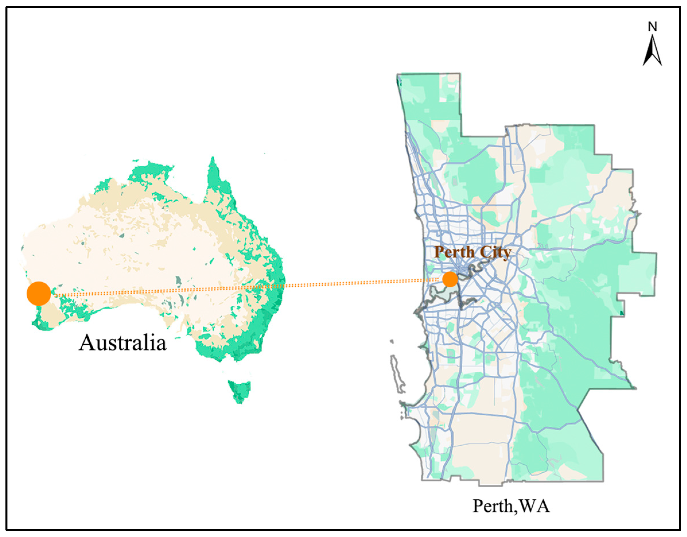
1.3. Study Area—Perth
1.4. Data and Pre-Processing
2. Methodology
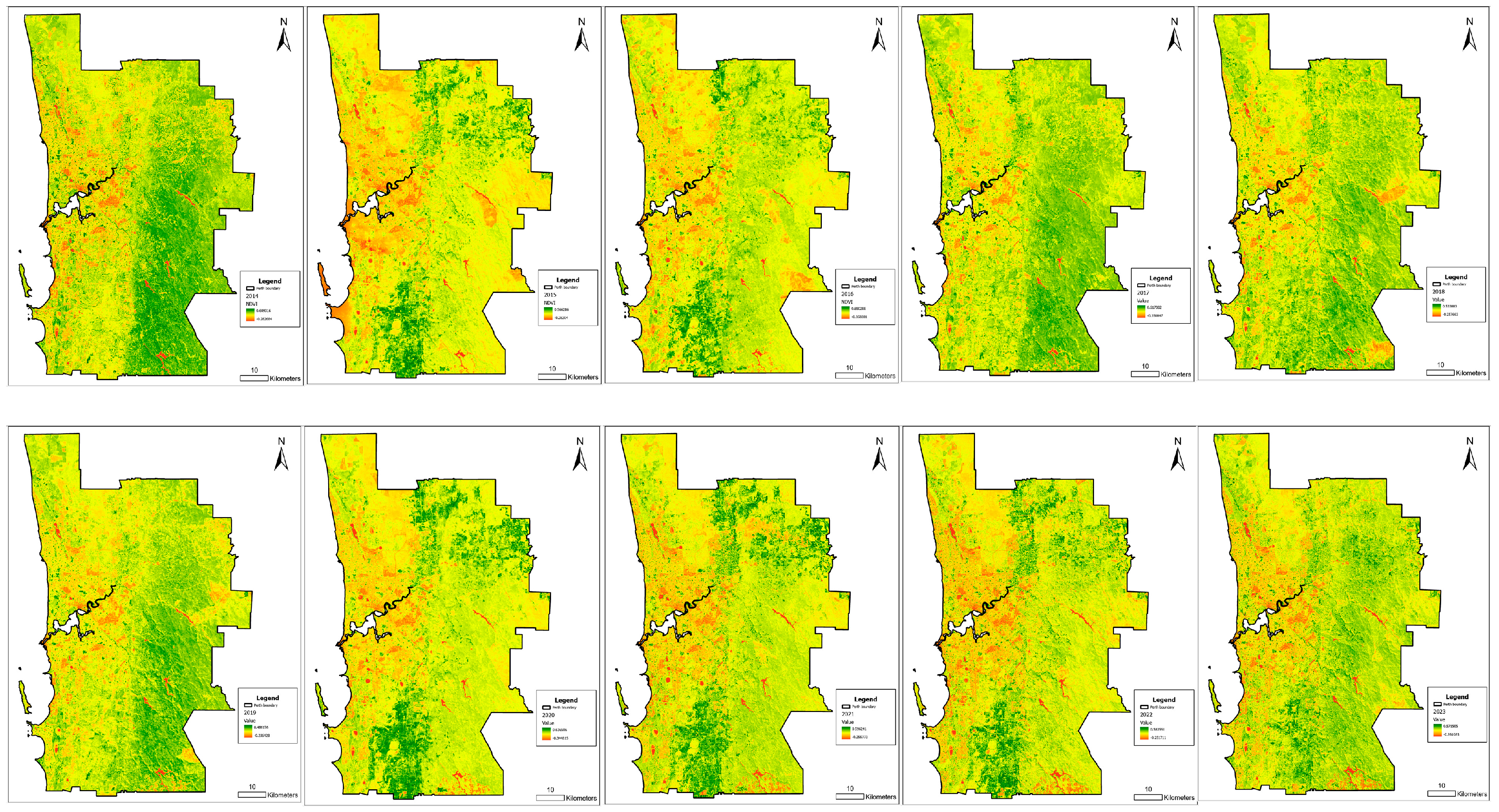
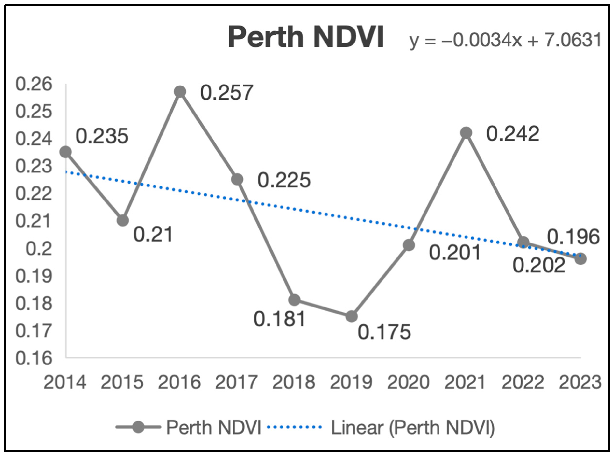
2.1. Stage 1: Trend of NDVI and LST in Perth over a 10-Year Period (2014–2023)
2.1.1. NDVI
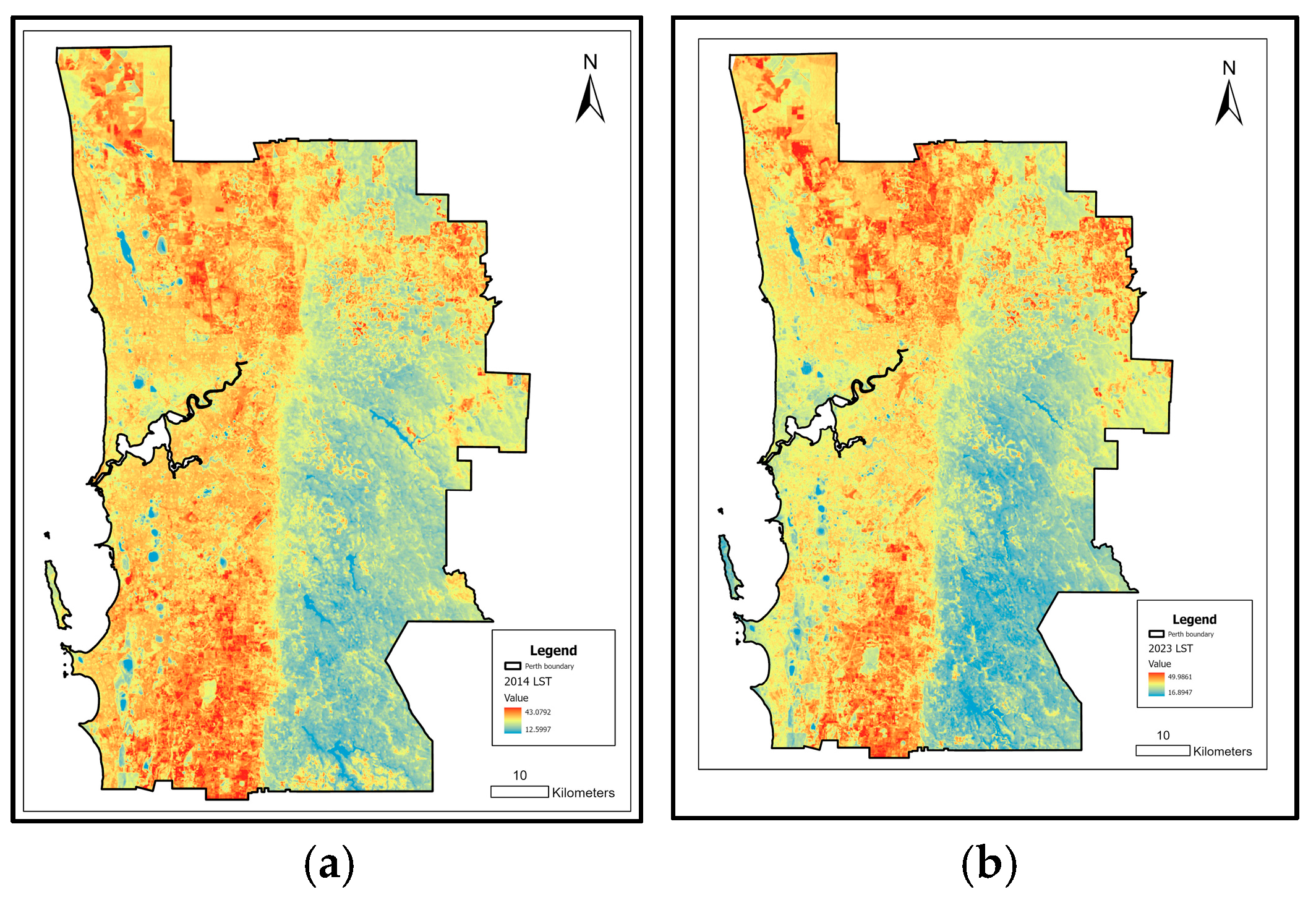
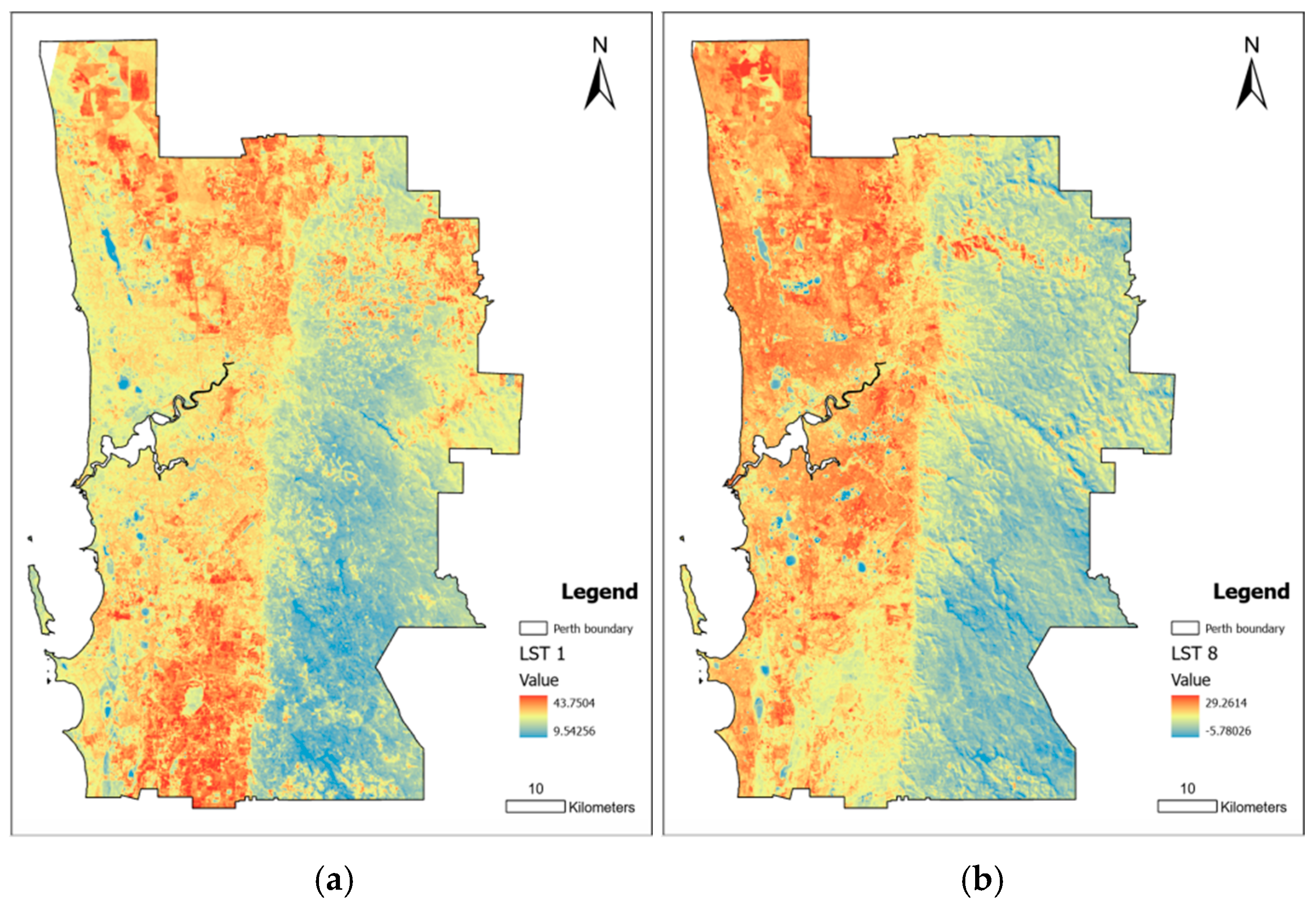
2.1.2. LST
2.1.3. Process and Results
2.2. Stage 2: Study the Relationship Between NDVI and Climate, Specifically Temperature and Precipitation
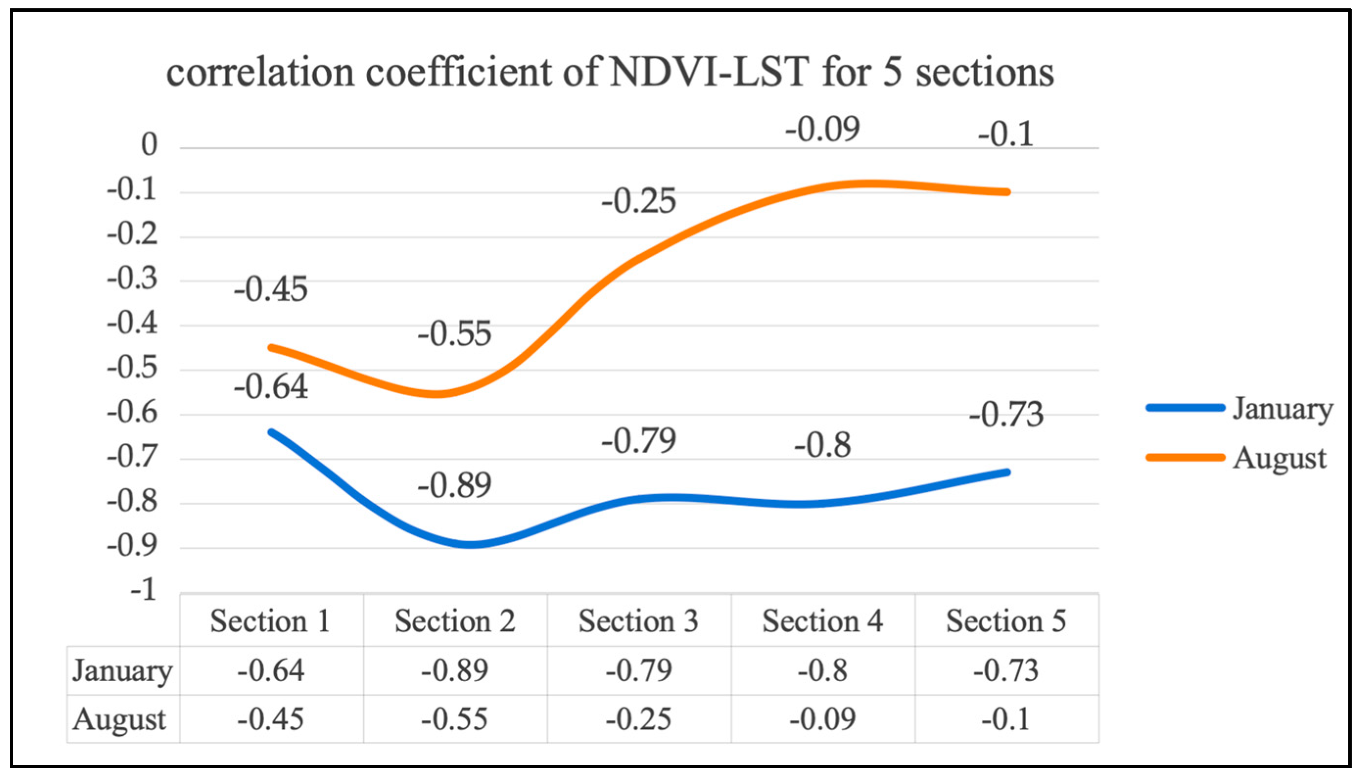
2.3. Stage 3: Understand the Relationship Between NDVI and LST Across the Seasons
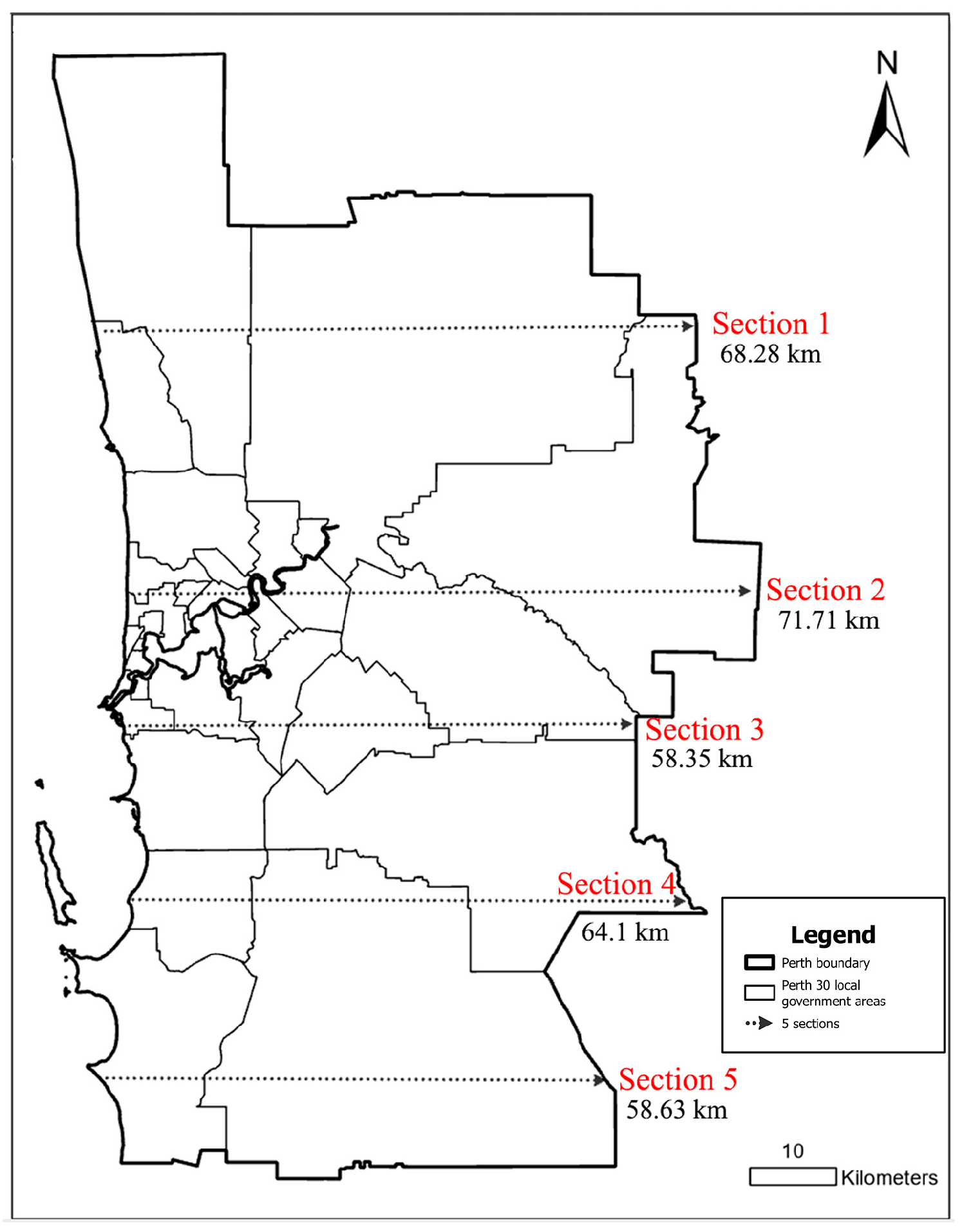
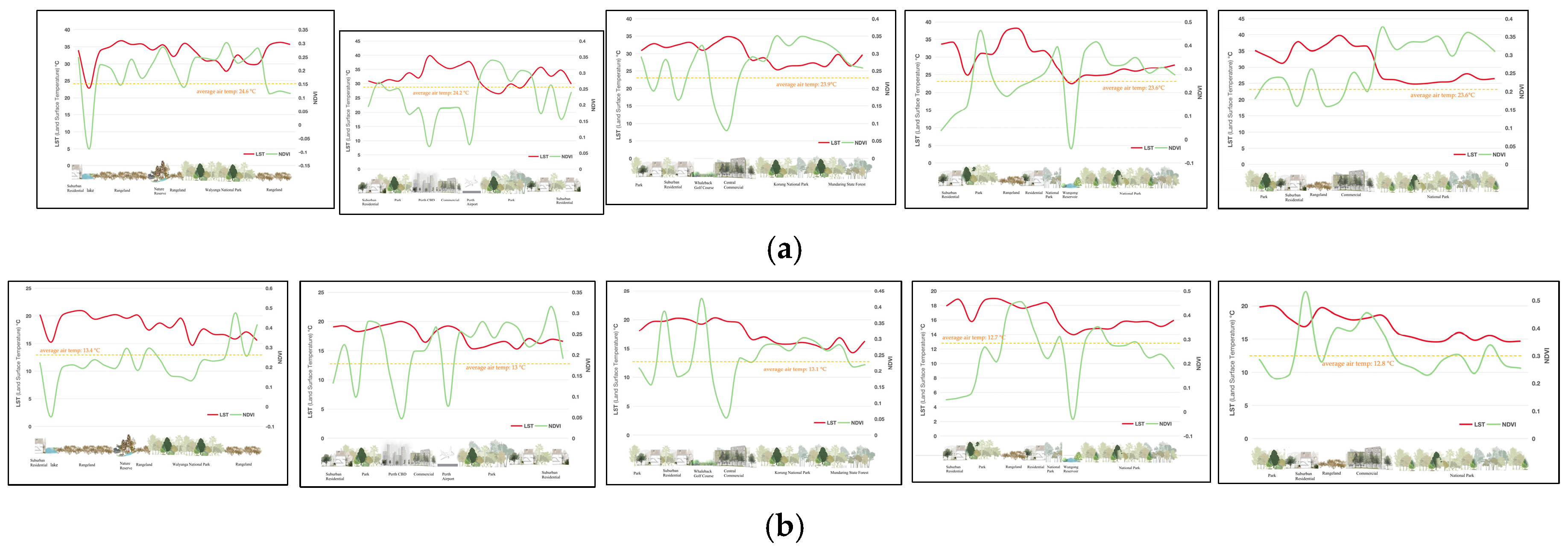
2.4. Stage 4: Study the Effect of LULC on NDVI and LST
3. Discussion
- (1)
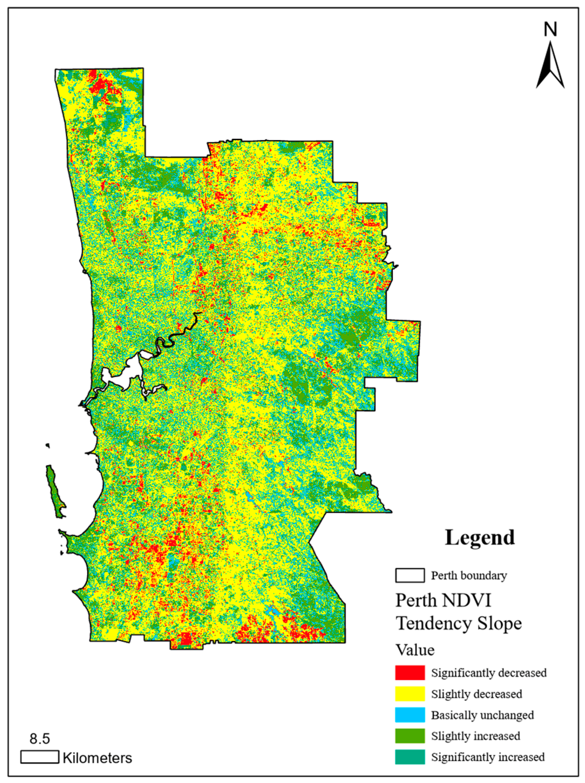
- From Stage 1, the observed decline in NDVI (55.4% of the study area) and concurrent rise in LST over the decade align with global trends where urban sprawl replaces green spaces with impervious surfaces, exacerbating UHI effects. The strong negative correlation between NDVI and LST (supported by previous work [36]) underscores vegetation’s role as a natural thermal regulator. Urban design that prioritizes NDVI enhancement, even in dense areas, can mitigate thermal stress, offering actionable strategies for sustainable city planning.
- (2)
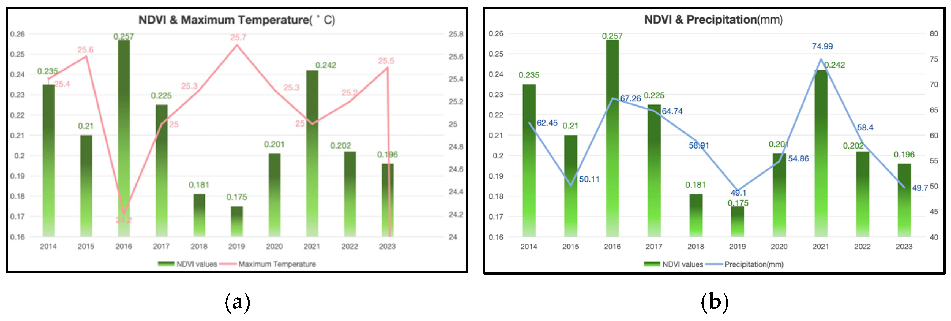
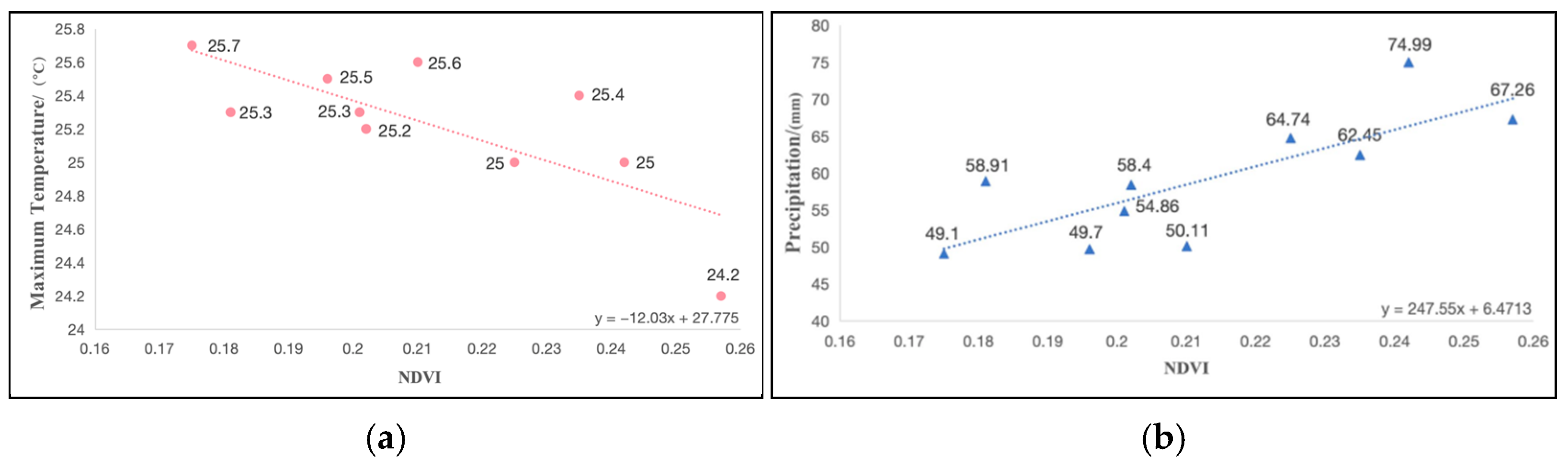
- From Stage 2, the significant correlations between NDVI and climatic variables (temperature: −0.754; precipitation: +0.779) highlight climate change as a dual-threat amplifier. Rising temperatures and altered precipitation patterns may compound vegetation loss caused by urbanization, creating feedback loops that intensify UHI. While these findings align with regional studies [37], they emphasize the urgency of integrating climate resilience into urban greening policies, particularly in semi-arid regions like Perth.
- (3)
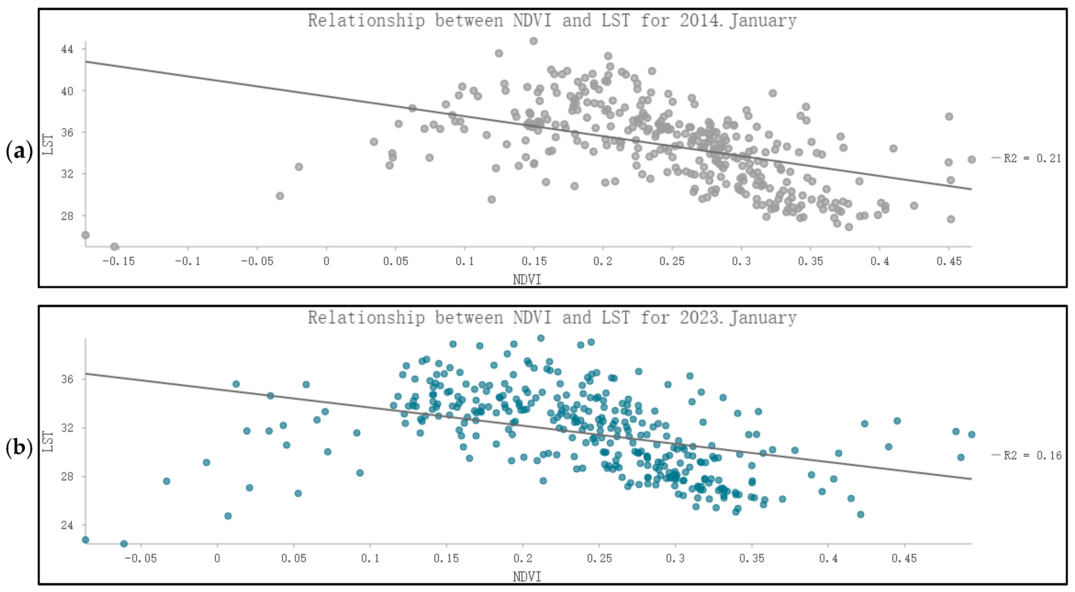
- From Stage 3, the stronger NDVI-LST correlation in summer (−0.5272) vs. winter (−0.1796) suggests seasonal vegetation activity and water availability mediate thermal regulation. Summer dryness reduces vegetation cooling efficiency, amplifying UHI during peak heat periods. This seasonality implies that UHI mitigation strategies, such as targeted irrigation or drought-resistant greening, will account for temporal variability in climate-vegetation interactions.
- (4)
- Urban density is not correlated with NDVI; Perth city has a lower NDVI than the suburbs. At the same time, in this study, LST is found to be correlated with NDVI, suggesting that increasing urban density is preferable to urban sprawl if greenery is used as a mitigating factor. This will allow the population to grow whilst reducing the urban footprint and maintaining a high NDVI within the city.
- (5)
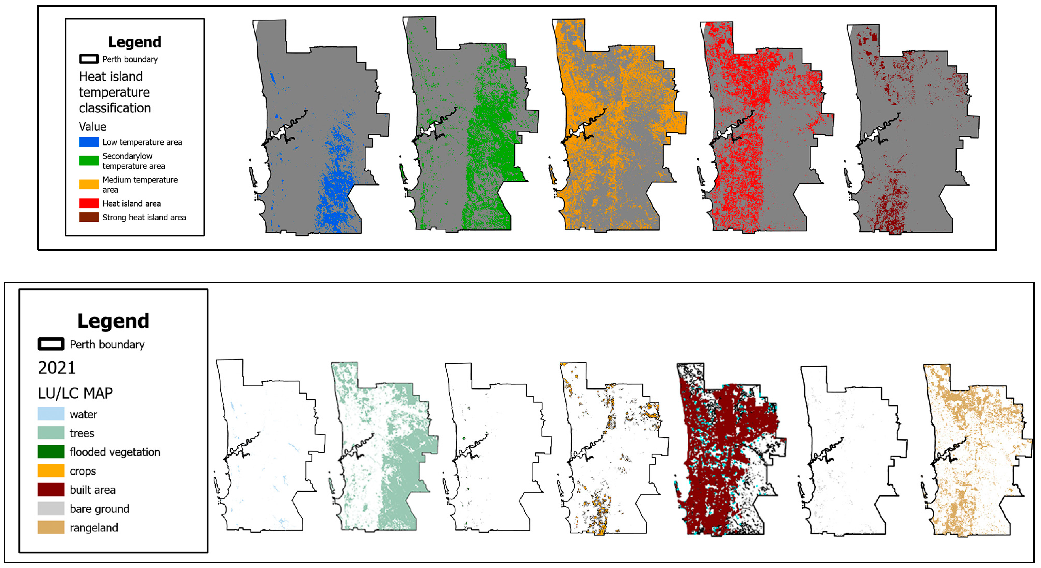
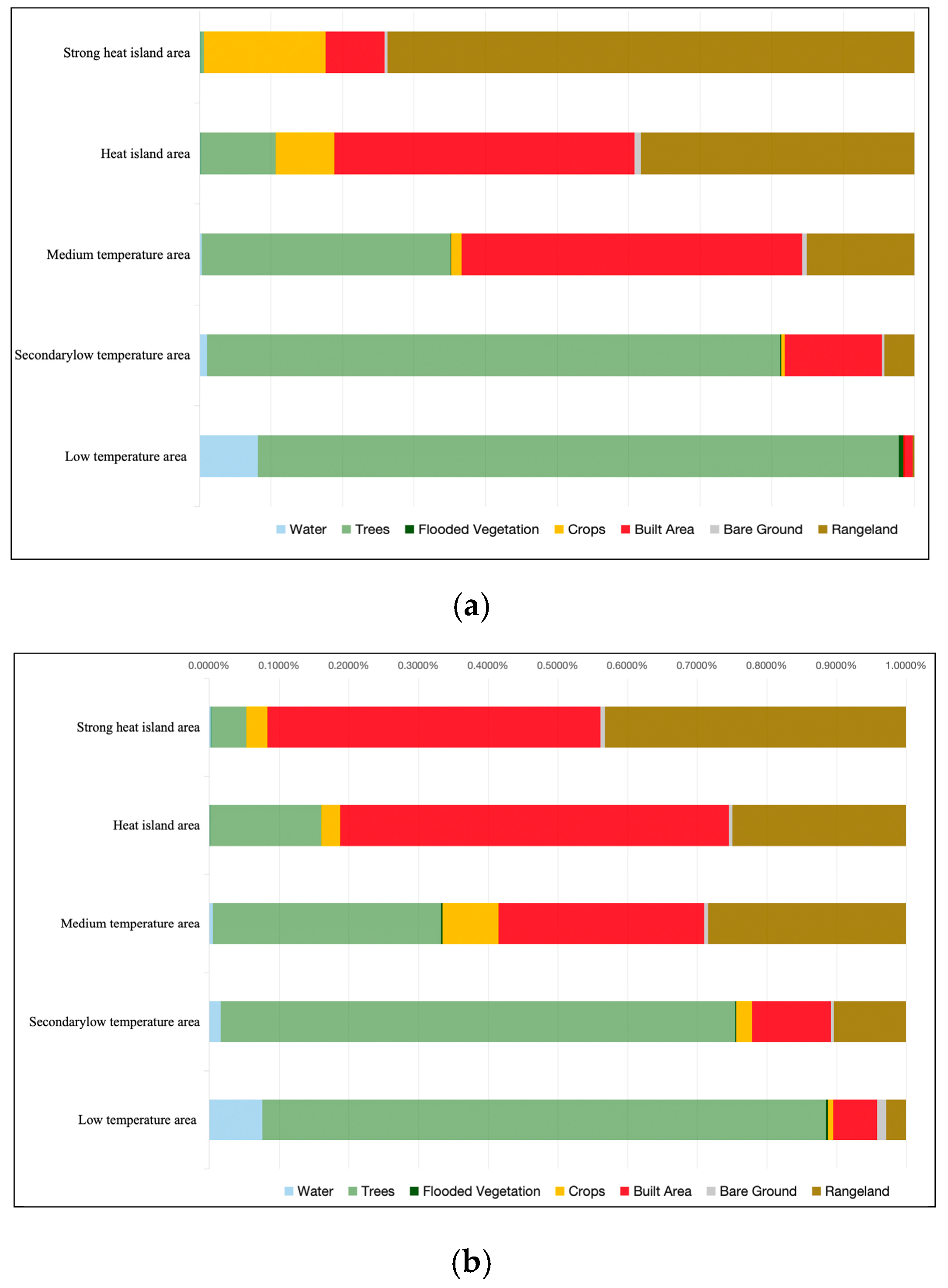
- In Stage 4, the medium and high temperature areas were mainly concentrated in urban dense areas and areas with low vegetation coverage, while the low temperature areas were mainly concentrated in areas with high vegetation coverage, such as forests. The results confirmed that areas with large vegetation coverage contributed significantly lower UHI values [38]. It was also confirmed by the LU/LC composition of heat island areas at all levels that areas with high tree and vegetation coverage have significantly lower surface temperatures (LST) and can provide “low temperature green islands” in the city, while built-up areas and low vegetation areas became the core components of high temperature areas.
- (6)
- Notably, rangelands emerged as unexpected contributors to summer UHI in Perth due to dry-season desiccation, challenging conventional views that non-urban vegetated areas uniformly cool cities. This finding calls for nuanced LU/LC management particularly in cities like Perth with long dry summers and arid natural landscapes.
4. Conclusions
Author Contributions
Funding
Data Availability Statement
Conflicts of Interest
References
- Desa, U.N. World Population Prospects 2022: Summary of Results; United Nations Department of Economic and Social Affairs: New York, NY, USA, 2022. [Google Scholar]
- The Intergovernmental Panel on Climate Change (IPCC). Climate Change 2007: Impacts, Adaptation and Vulnerability; Cambridge University Press: Genebra, Switzerland, 2001. [Google Scholar]
- Jabbar, H.K.; Hamoodi, M.N.; Al-Hameedawi, A.N. UHIs: A review of contributing factors, effects and data. In IOP Conference Series: Earth and Environmental Science; IOP Publishing: Bristol, UK, 2023; Volume 1129, p. 012038. [Google Scholar]
- Fu, J.; Dupre, K.; Tavares, S.; King, D.; Banhalmi-Zakar, Z. Optimized greenery configuration to mitigate urban heat: A decade systematic review. Front. Arch. Res. 2022, 11, 466–491. [Google Scholar] [CrossRef]
- Bowler, D.E.; Buyung-Ali, L.; Knight, T.M.; Pullin, A.S. Urban greening to cool towns and cities: A systematic review of the empirical evidence. Landsc. Urban Plan. 2010, 97, 147–155. [Google Scholar] [CrossRef]
- Zölch, T.; Maderspacher, J.; Wamsler, C.; Pauleit, S. Using green infrastructure for urban climate-proofing: An evaluation of heat mitigation measures at the micro-scale. Urban For. Urban Green. 2016, 20, 305–316. [Google Scholar] [CrossRef]
- Brovkin, V. Climate-vegetation interaction. J. Phys. IV 2002, 12, 57–72. [Google Scholar] [CrossRef]
- Ellison, D.; Morris, C.E.; Locatelli, B.; Sheil, D.; Cohen, J.; Murdiyarso, D.; Gutierrez, V.; van Noordwijk, M.; Creed, I.F.; Pokorny, J.; et al. Trees, forests and water: Cool insights for a hot world. Glob. Environ. Chang. 2017, 43, 51–61. [Google Scholar] [CrossRef]
- Sheil, D.; Murdiyarso, D. How forests attract rain: An examination of a new hypothesis. Bioscience 2009, 59, 341–347. [Google Scholar] [CrossRef]
- Lima Alves, E.D.; Lopes, A. The UHI effect and the role of vegetation to address the negative impacts of local climate changes in a small Brazilian City. Atmosphere 2017, 8, 18. [Google Scholar] [CrossRef]
- Buyantuyev, A.; Wu, J. Urban heat islands and landscape heterogeneity: Linking spatiotemporal variations in surface temperatures to land-cover and socioeconomic patterns. Landsc. Ecol. 2010, 25, 17–33. [Google Scholar] [CrossRef]
- Weng, Q.; Lu, D.; Schubring, J. Estimation of land surface temperature—Vegetation abundance relationship for UHI studies. Remote Sens. Env. 2004, 89, 467–483. [Google Scholar] [CrossRef]
- Dewan, A.M.; Corner, R.J. Impact of land use and land cover changes on urban land surface temperature. In Dhaka Megacity: Geospatial Perspectives on Urbanisation, Environment and Health; Springer: Dordrecht, The Netherlands, 2013; pp. 219–238. [Google Scholar]
- Weng, Q.; Fu, P.; Gao, F. Generating daily land surface temperature at Landsat resolution by fusing Landsat and MODIS data. Remote Sens. Environ. 2014, 145, 55–67. [Google Scholar] [CrossRef]
- Nichol, J. An emissivity modulation method for spatial enhancement of thermal satellite images in UHI analysis. Photogramm. Eng. Remote Sens. 2009, 75, 547–556. [Google Scholar] [CrossRef]
- Sobrino, J.A.; Oltra-Carrió, R.; Sòria, G.; Bianchi, R.; Paganini, M. Impact of spatial resolution and satellite overpass time on evaluation of the surface urban heat island effects. Remote Sens. Environ. 2012, 117, 50–56. [Google Scholar] [CrossRef]
- City of Perth Annual Report 2020/21. Available online: https://perth.wa.gov.au/council/reports-and-important-documents (accessed on 21 February 2025).
- Perth, Australian Metro Area Population 1950–2050. Available online: https://www.macrotrends.net/global-metrics/cities/206172/perth/population (accessed on 4 May 2025).
- Climate Change 2022: Impacts, Adaptation and Vulnerability. Available online: https://www.ipcc.ch/report/ar6/wg2/ (accessed on 4 May 2025).
- Vigneshwaran, S.; Vasantha Kumar, S. Extraction of built-up area using high resolution sentinel-2a and google satellite imagery. Int. Arch. Photogramm. Remote Sens. Spat. Inf. Sci. 2018, 42, 165–169. [Google Scholar] [CrossRef]
- Tucker, C.J. Red and photographic infrared linear combinations for monitoring vegetation. Remote Sens. Environ. 1979, 8, 127–150. [Google Scholar] [CrossRef]
- Huang, S.; Tang, L.; Hupy, J.P.; Wang, Y.; Shao, G. A commentary review on the use of NDVI (NDVI) in the era of popular remote sensing. J. For. Res. 2021, 32, 1–6. [Google Scholar] [CrossRef]
- Pettorelli, N.; Vik, J.O.; Mysterud, A.; Gaillard, J.M.; Tucker, C.J.; Stenseth, N.C. Using the satellite-derived NDVI to assess ecological responses to environmental change. Trends Ecol. Evol. 2005, 20, 503–510. [Google Scholar] [CrossRef]
- Piao, S.; Friedlingstein, P.; Ciais, P.; Viovy, N.; Demarty, J. Growing season extension and its impact on terrestrial carbon cycle in the Northern Hemisphere over the past 2 decades. Glob. Biogeochem. Cycles 2007, 21. [Google Scholar] [CrossRef]
- Colombo, R.; Bellingeri, D.; Fasolini, D.; Marino, C.M. Retrieval of leaf area index in different vegetation types using high resolution satellite data. Remote Sens. Environ. 2003, 86, 120–131. [Google Scholar] [CrossRef]
- Fan, L.Y.; Gao, Y.Z.; Brück, H.E.B.C.; Bernhofer, C. Investigating the relationship between NDVI and LAI in semi-arid grassland in Inner Mongolia using in-situ measurements. Theor. Appl. Climatol. 2009, 95, 151–156. [Google Scholar] [CrossRef]
- Lu, L.; Li, X.; Ma, M.G.; Che, T.; Huang, C.L.; Veroustraete, F.; Bogaert, J.; Dong, Q.; Ceulemans, R. Investigating relationship between Landsat ETM+ data and LAI in a semi-arid grassland of Northwest China. In Proceedings of the IGARSS 2004. 2004 IEEE International Geoscience and Remote Sensing Symposium, Anchorage, AK, USA, 20–24 September 2004; Volume 6, pp. 3622–3625. [Google Scholar]
- Gitelson, A.A.; Viña, A.; Arkebauer, T.J.; Rundquist, D.C.; Keydan, G.; Leavitt, B. Remote estimation of leaf area index and green leaf biomass in maize canopies. Geophys. Res. Lett. 2003, 30. [Google Scholar] [CrossRef]
- Sun, P.S.; Liu, S.R.; Liu, J.T.; Li, C.; Lin, Y.; Jiang, H. Derivation and validation of leaf area index maps using NDVI data of different resolution satellite imageries. Acta Ecol. Sin. 2006, 26, 3826–3834. [Google Scholar]
- Li, Z.L.; Tang, B.H.; Wu, H.; Ren, H.; Yan, G.; Wan, Z.; Trigo, I.F.; Sobrino, J.A. Satellite-derived land surface temperature: Current status and perspectives. Remote Sens. Environ. 2013, 131, 14–37. [Google Scholar] [CrossRef]
- D’Allestro, P.; Parente, C. GIS application for NDVI calculation using Landsat 8 OLI images. Int. J. Appl. Eng. Res. 2015, 10, 42099–42102. [Google Scholar]
- Oguz, H. LST calculator: A program for retrieving land surface temperature from Landsat TM/ETM+ imagery. Environ. Eng. Manag. J. 2013, 12, 549–555. [Google Scholar] [CrossRef]
- Adler, J.; Parmryd, I. Quantifying colocalization by correlation: The Pearson correlation coefficient is superior to the Mander’s overlap coefficient. Cytom. Part A 2010, 77, 733–742. [Google Scholar] [CrossRef]
- Quan, J.; Chen, Y.; Zhan, W.; Wang, J.; Voogt, J.; Wang, M. Multi-temporal trajectory of the urban heat island centroid in Beijing, China based on a Gaussian volume model. Remote Sens. Environ. 2014, 149, 33–46. [Google Scholar] [CrossRef]
- Xu, H.; Chen, Y.; Dan, S.; Qiu, W. Dynamical monitoring and evaluation methods to urban heat island effects based on RS&GIS. Procedia Environ. Sci. 2011, 10, 1228–1237. [Google Scholar]
- Karnieli, A.; Agam, N.; Pinker, R.T.; Anderson, M.; Imhoff, M.L.; Gutman, G.G.; Panov, N.; Goldberg, A. Use of NDVI and land surface temperature for drought assessment: Merits and limitations. J. Clim. 2010, 23, 618–633. [Google Scholar] [CrossRef]
- Ding, M.; Zhang, Y.; Liu, L.; Zhang, W.; Wang, Z.; Bai, W. The relationship between NDVI and precipitation on the Tibetan Plateau. J. Geogr. Sci. 2007, 17, 259–268. [Google Scholar] [CrossRef]
- Ukoha, P.A.; Okonkwo, S.J.; Adewoye, A.R. Evaluation of the Impact of Urban Forestry on UHI. J. Appl. Sci. Environ. Manag. 2023, 27, 893–898. [Google Scholar]
- City of Perth Urban Greening Strategy 2023–2036. Available online: https://perth.wa.gov.au/community/sustainability-hub/urban-greening (accessed on 20 April 2025).


| Land Cover | Regression | RMSE | |
|---|---|---|---|
| Coniferous forest | LAI = 1.8 (NDVI + 0.069)/(0.815 − NDVI) | 0.346 | 0.599 |
| Mixed forest | LAI = 4.686NDVI/(1.181 − NDVI) | 0.592 | 0.536 |
| Temperate deciduous shrub | LAI = 8.547NDVI − 0.932 | 0.583 | 0.384 |
| Alpine evergreen shrub | LAI = 9.174NDVI − 0.648 | 0.715 | 0.500 |
| Broadleaved forest | LAI = 7.813NDVI + 0.789 | 0.732 | 0.461 |
| Crop land | LAI = 6.211NDVI − 1.088 | 0.760 | 0.529 |
| Alpine meadow | LAI = 3.968NDVI + 1.202 | 0.871 | 0.470 |
| Perth | |
|---|---|
| Significantly decreased (−0.085 ≤ s ≤ −0.01) | 5.6% |
| Slightly decreased (−0.01 ≤ s ≤ −0.001) | 55.4% |
| Basically unchanged (−0.001 ≤ s ≤ 0.001) | 20.1% |
| Slightly increased (0.001 ≤ s ≤ 0.01) | 17.7% |
| Significantly increased (0.01 ≤ s ≤ 0.081) | 1.1% |
| LST (°C) | MAX (°C) | MIN (°C) | MEAN (°C) |
|---|---|---|---|
| 2014 | 43.079 | 12.6 | 31.732 |
| 2023 | 49.986 | 16.895 | 34.771 |
| Year 2014 | Year 2023 | |
|---|---|---|
| Correlation coefficient (r) | −0.456 | −0.396 |
| Year | Perth Monthly Precipitation (mm) | Perth Mean Maximum Temperature (°C) |
|---|---|---|
| 2014 | 62.45 | 25.4 |
| 2015 | 50.11 | 25.6 |
| 2016 | 67.26 | 24.2 |
| 2017 | 64.74 | 25 |
| 2018 | 58.91 | 25.3 |
| 2019 | 49.1 | 25.7 |
| 2020 | 54.86 | 25.3 |
| 2021 | 74.99 | 25 |
| 2022 | 58.4 | 25.2 |
| 2023 | 49.7 | 25.5 |
| Perth Monthly Precipitation (mm) | Perth Mean Maximum Temperature (°C) | |
|---|---|---|
| Correlation coefficient with NDVI (r) | 0.779 | −0.754 |
| Number | Crossed LGAs | LU/LC |
|---|---|---|
| Section 1 | Joondalup, Swan, Mundaring | Suburban Residential, Mariginiup Lake, Rangeland, Nature Reserve, Rangeland, Walyunga National Park, Rangeland |
| Section 2 | Cambridge, Netlands, Subiaco, Perth, Belmont, Kalamunda, Mundaring | Suburban Residential, Park, Perth CBD, Commercial, Perth Airport, National Park, Suburban Residential |
| Section 3 | Fremantle, Melville, Canning, Gosnells, Kalamunda | Park, Suburban Residential, Whaleback Golf Course, Central Commercial, Korung National Park, Mundaring State Forest |
| Section 4 | Kwinana, Serpentine-Jarrahdale, Armadale | Suburban Residential, Park, Rangeland, Residential, National Park, Wungong Reservoir, National Park |
| Section 5 | Rockingham, Serpentine-Jarrahdale | Park, Suburban Residential, Rangeland, Commercial, National Park |
| Classification | Interval of Temperature Classification |
|---|---|
| Strong heat island area | T > μ + 1.5σ |
| Heat island area | μ + 0.5σ < T ≤ μ + 1.5σ |
| Medium temperature area | μ − 0.5σ ≤ T ≤ μ + 0.5σ |
| Secondary low temperature area | μ − 1.5σ ≤ T < μ − 0.5σ |
| Low temperature area | T < μ − 1.5σ |
Disclaimer/Publisher’s Note: The statements, opinions and data contained in all publications are solely those of the individual author(s) and contributor(s) and not of MDPI and/or the editor(s). MDPI and/or the editor(s) disclaim responsibility for any injury to people or property resulting from any ideas, methods, instructions or products referred to in the content. |
© 2025 by the authors. Licensee MDPI, Basel, Switzerland. This article is an open access article distributed under the terms and conditions of the Creative Commons Attribution (CC BY) license (https://creativecommons.org/licenses/by/4.0/).
Share and Cite
Ma, X.; Ong, B.L. Optimizing Urban Greenery for Climate Resilience: A Case Study in Perth, Australia. Land 2025, 14, 1088. https://doi.org/10.3390/land14051088
Ma X, Ong BL. Optimizing Urban Greenery for Climate Resilience: A Case Study in Perth, Australia. Land. 2025; 14(5):1088. https://doi.org/10.3390/land14051088
Chicago/Turabian StyleMa, Xiaoqi, and Boon Lay Ong. 2025. "Optimizing Urban Greenery for Climate Resilience: A Case Study in Perth, Australia" Land 14, no. 5: 1088. https://doi.org/10.3390/land14051088
APA StyleMa, X., & Ong, B. L. (2025). Optimizing Urban Greenery for Climate Resilience: A Case Study in Perth, Australia. Land, 14(5), 1088. https://doi.org/10.3390/land14051088