
Optimizing Landscape Patterns for Tea Plantation Agroecosystems: A Case Study of an Important Agricultural Heritage System in Enshi, China


Abstract
1. Introduction
2. Materials and Methods
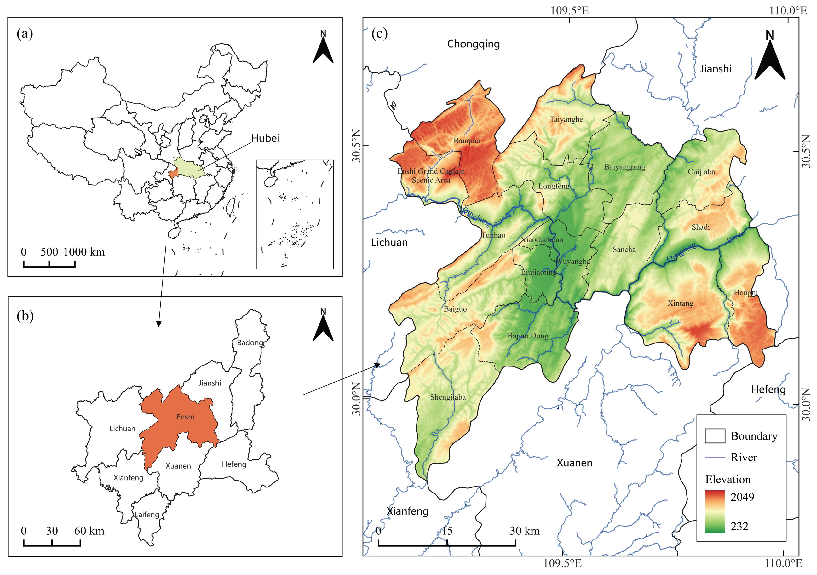
2.1. Study Area
2.2. Data Sources
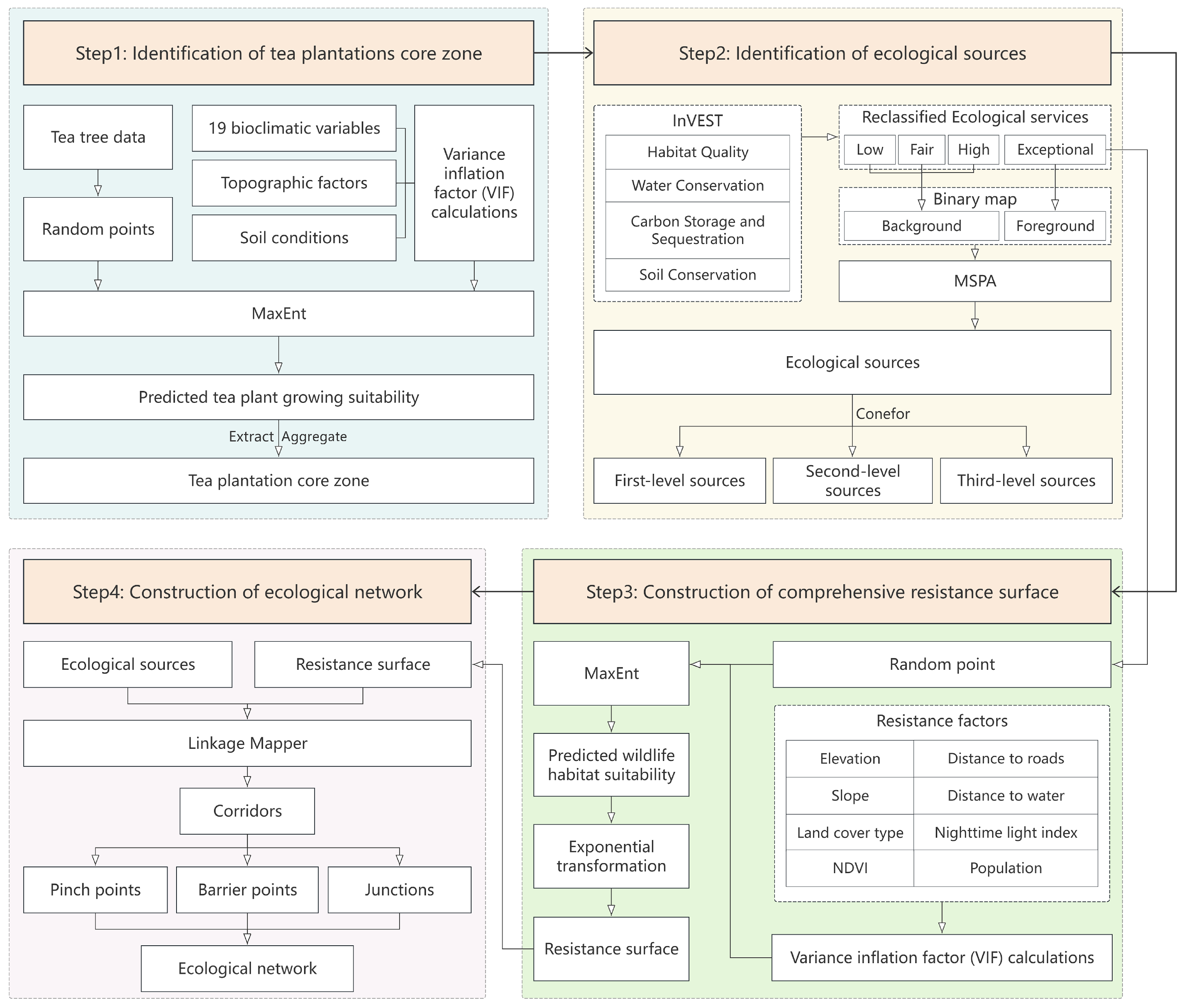
2.3. Methodology
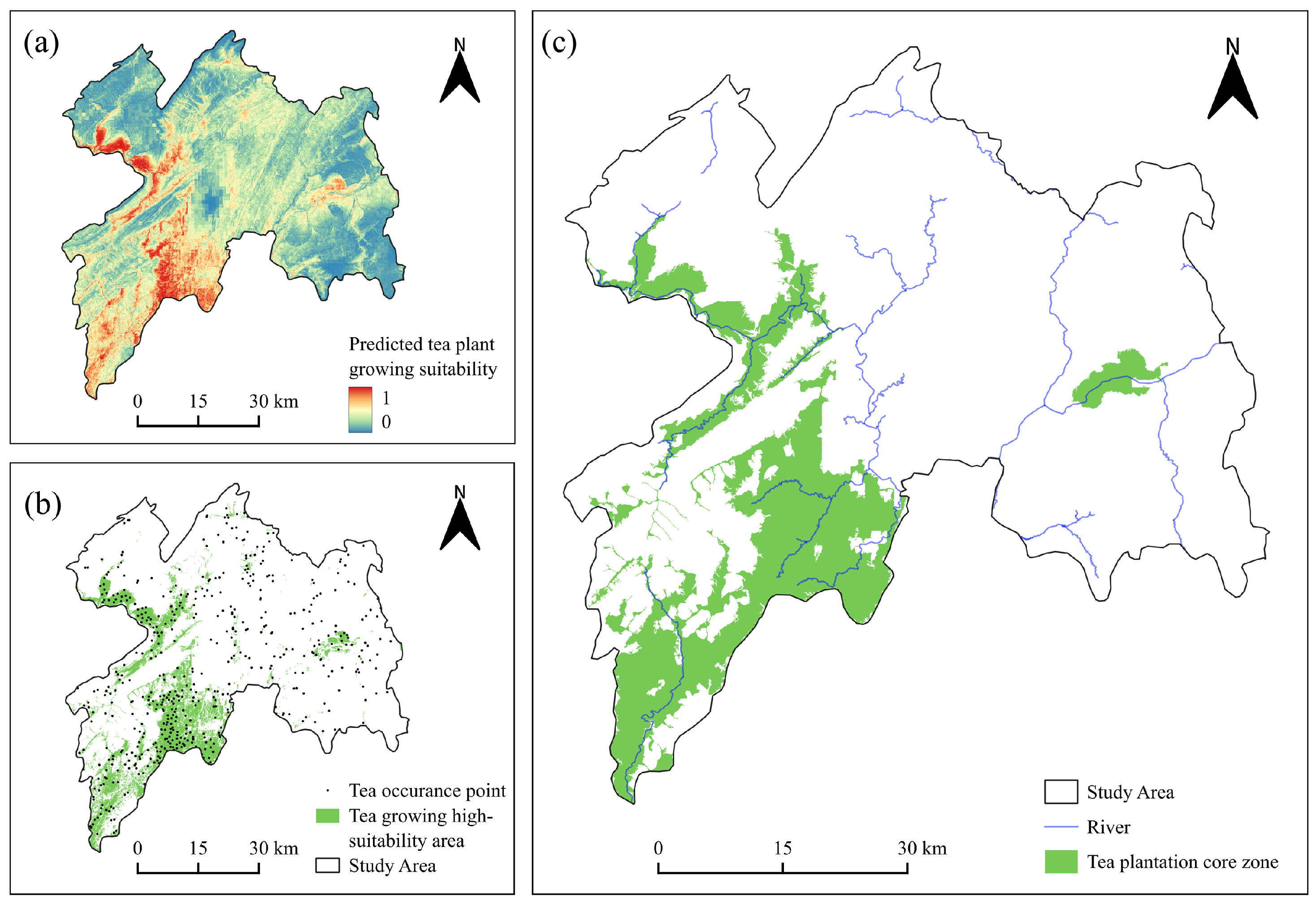
2.3.1. Identification of Tea Plantation Core Zone
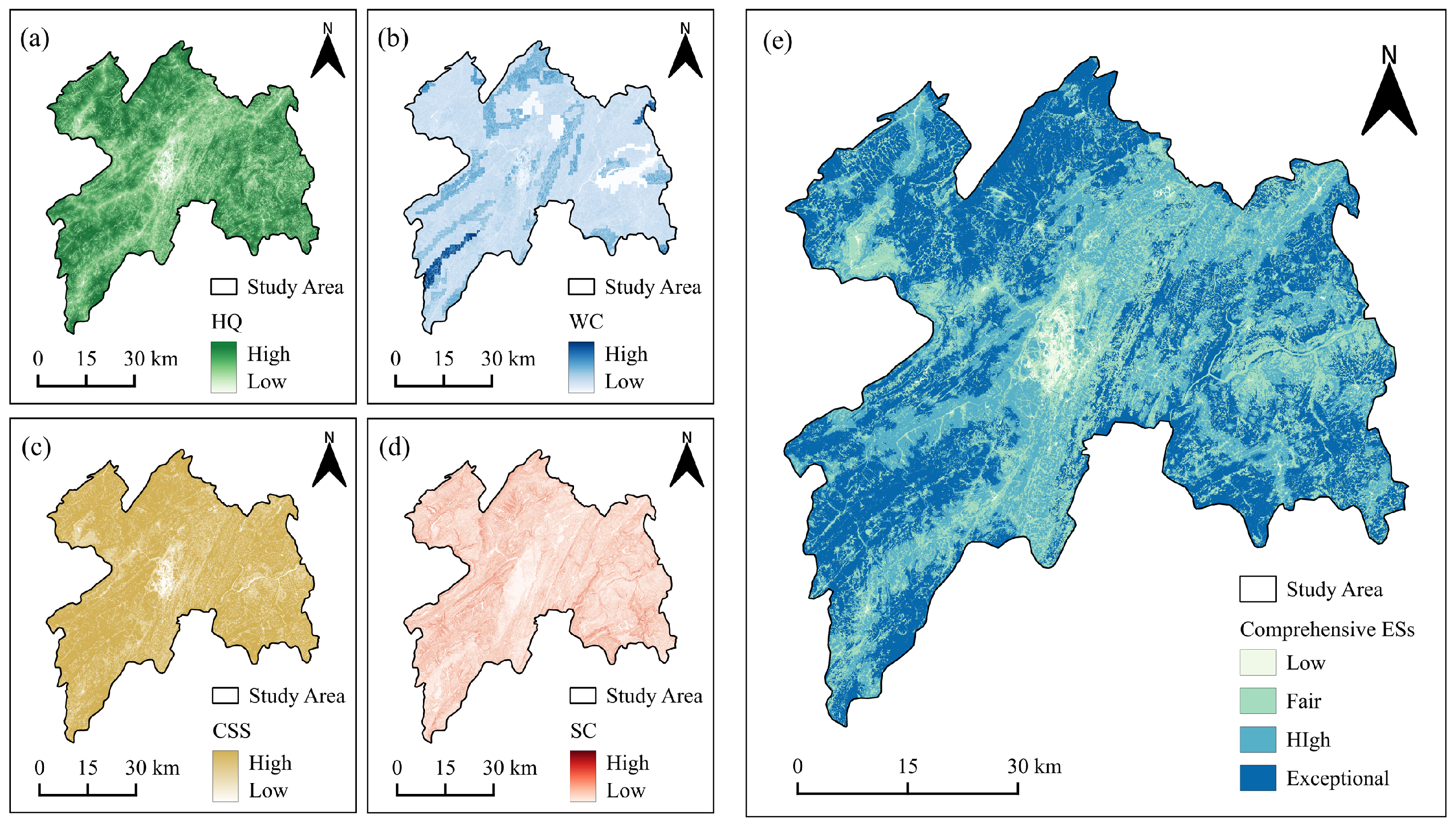
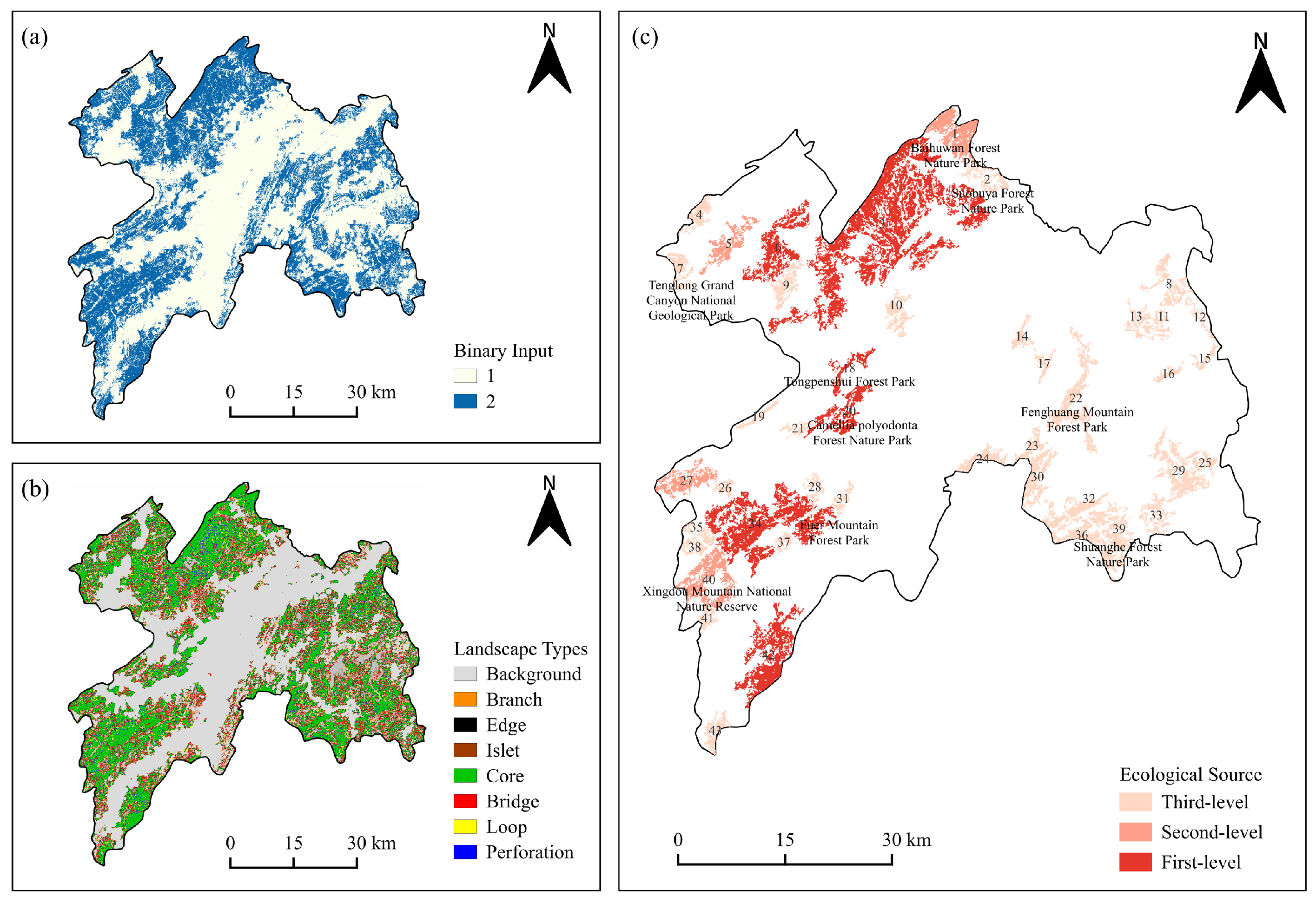
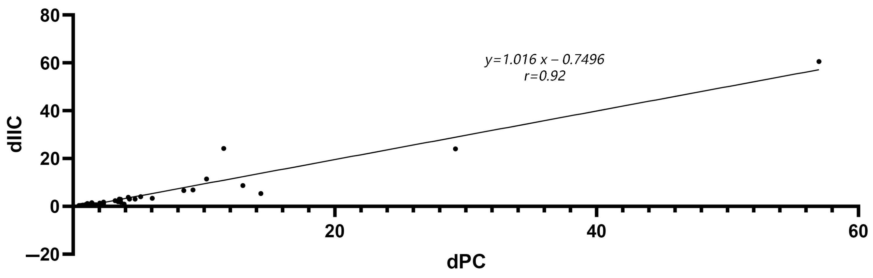
2.3.2. Identification of Ecological Sources
- (1)
- Habitat Quality
- (2)
- Water Conservation
- (3)
- Carbon Storage and Sequestration
- (4)
- Soil Conservation
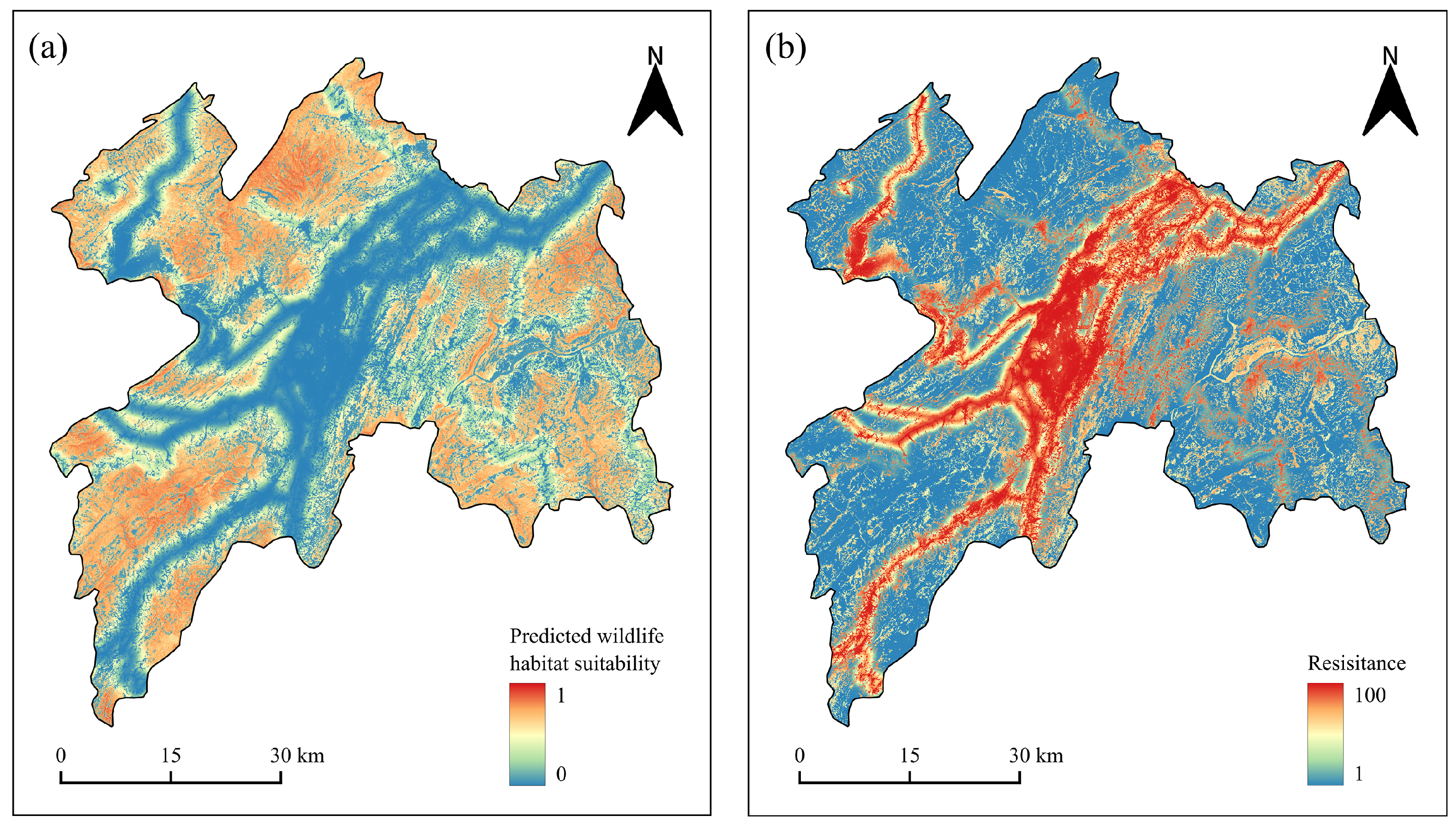
2.3.3. Construction of Comprehensive Resistance Surface
2.3.4. Construction of Ecological Network
2.3.5. Identification of Ecological Nodes
3. Result
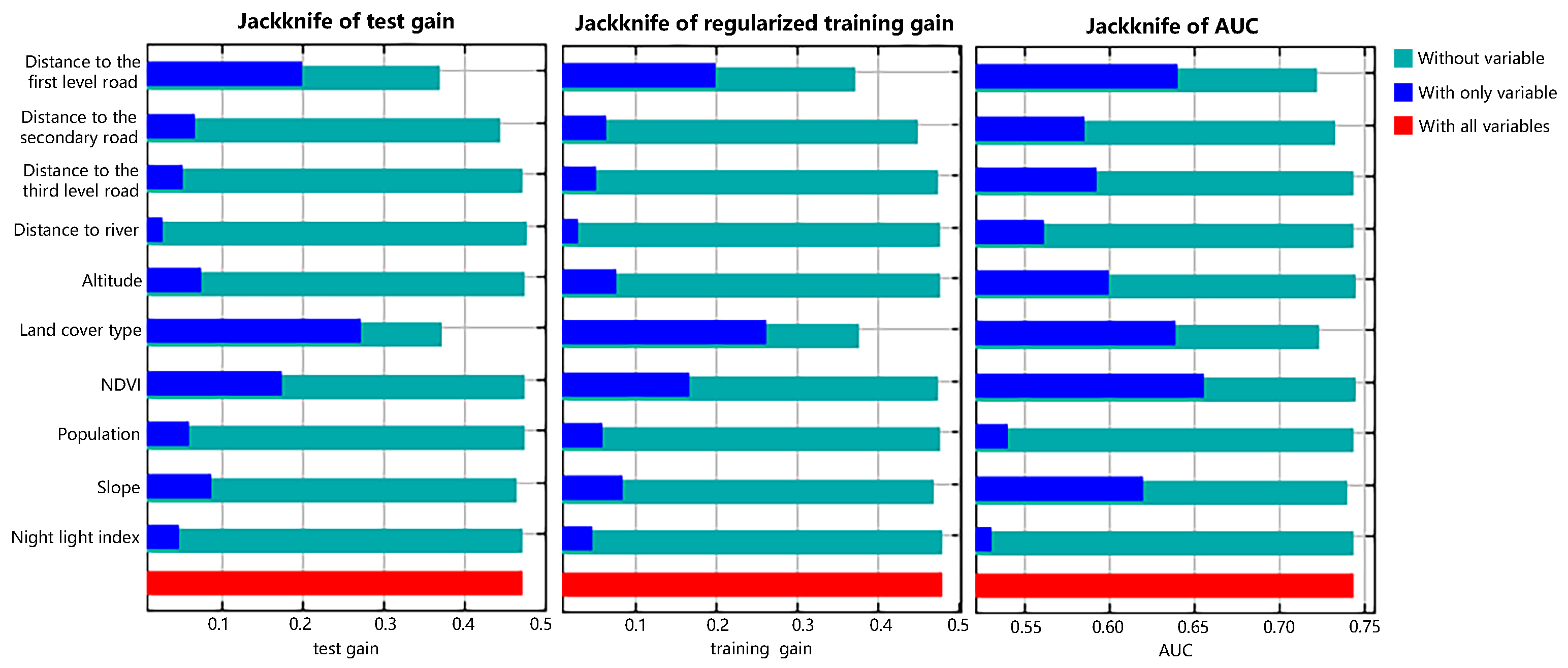
3.1. Tea Plantation Core Zone
3.2. Ecological Sources
3.3. Comprehensive Resistance Surface
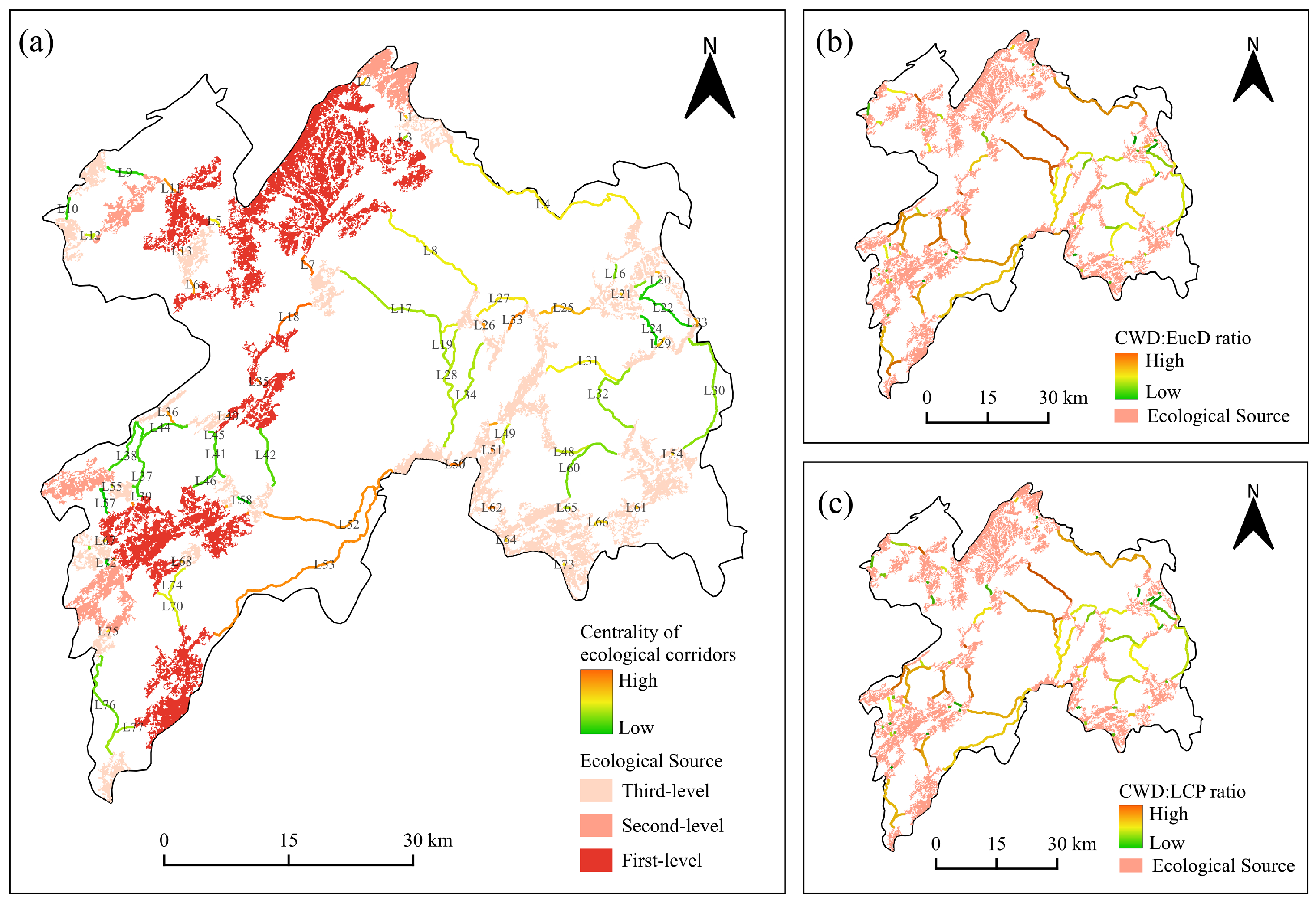
3.4. Ecological Corridors
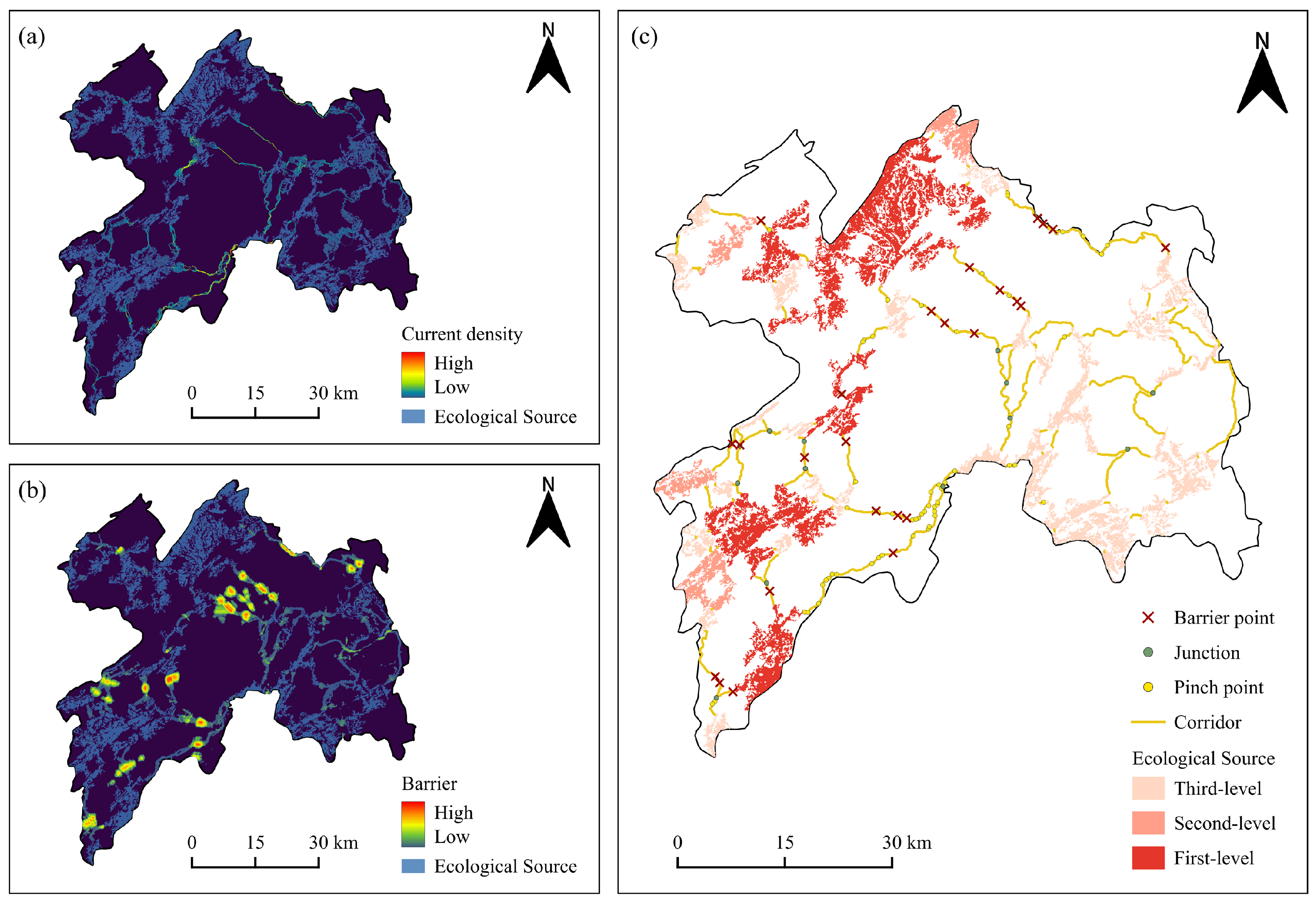
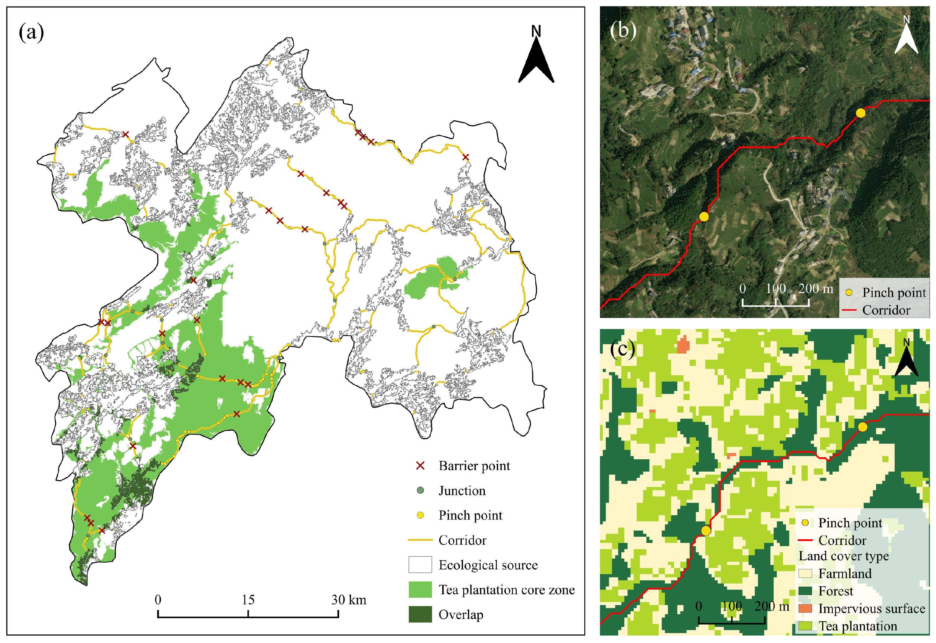
3.5. Ecological Nodes
4. Discussion
4.1. Distribution of Tea Plantations
4.2. Ecosystem Service Value and Resistance Surface
4.3. Ecological Benefits of Tea Fields
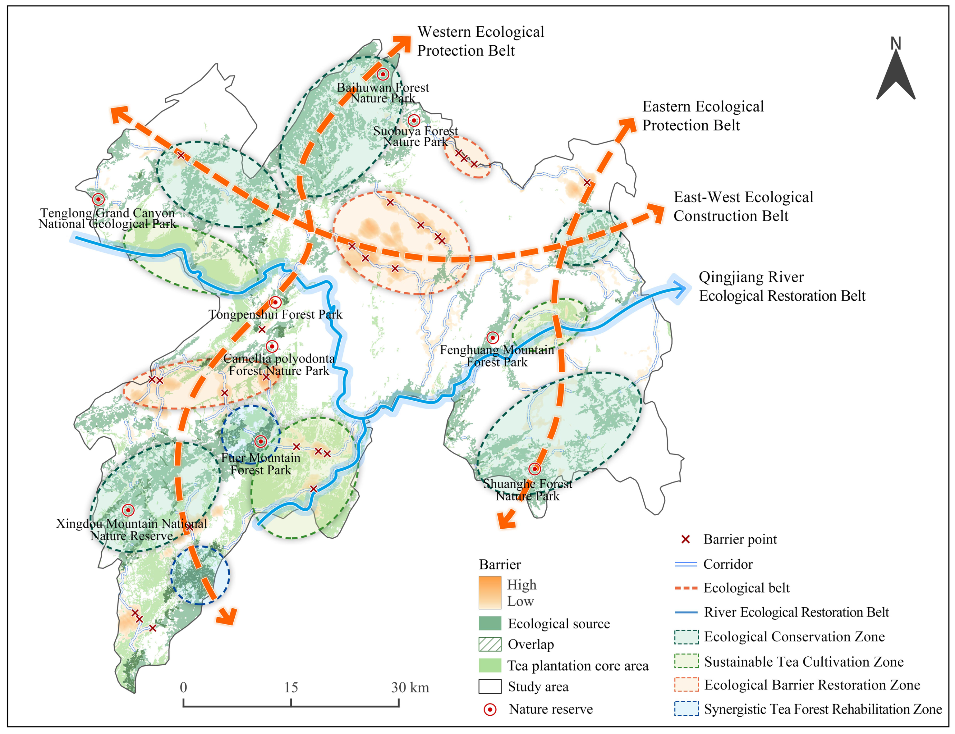
4.4. Landscape Pattern Optimization Approach
4.5. Other Limitations and Future Research Priorities
5. Conclusions
Author Contributions
Funding
Data Availability Statement
Acknowledgments
Conflicts of Interest
Appendix A

| Code | Biological Climate Variable | Code | Biological Climate Variable |
|---|---|---|---|
| Bio 1 | Annual Mean Temperature (°C) | Bio 11 | Mean Temperature of Coldest Quarter (°C) |
| Bio 2 | Mean Diurnal Range (°C) | Bio 12 | Annual Precipitation/mm |
| Bio 3 | Isothermality (bio2/bio7) | Bio 13 | Precipitation of Wettest Month/mm |
| Bio 4 | Temperature seasonality | Bio 14 | Precipitation of Driest Month/mm |
| Bio 5 | Max Temperature of Warmest Month (°C) | Bio 15 | Precipitation Seasonality/mm |
| Bio 6 | Min Temperature of Coldest Month (°C) | Bio 16 | Precipitation of Wettest Quarter/mm |
| Bio 7 | Temperature Annual Range (°C) | Bio 17 | Precipitation of Driest Quarter/mm |
| Bio 8 | Mean Temperature of Wettest Quarter (°C) | Bio 18 | Precipitation of Warmest Quarter/mm |
| Bio 9 | Mean Temperature of Driest Quarter (°C) | Bio 19 | Precipitation of Coldest Quarter/mm |
| Bio 10 | Mean Temperature of Warmest Quarter (°C) |
| Threat Factor | Maximum Impact Distance/km | Weight | Decay Type |
|---|---|---|---|
| Farmland | 2.00 | 0.50 | Exponential |
| Tea plantation | 2.00 | 0.30 | Exponential |
| Impervious surface | 6.00 | 0.80 | Exponential |
| First-level road | 3.00 | 0.50 | Linear |
| Secondary road | 1.50 | 0.40 | Linear |
| Third-level road | 0.50 | 0.20 | Exponential |
| Land Use Type | Habitat Suitability | Farmland | Impervious Surface | Tea Plantation | First-Level Road | Secondary Road | Third-Level Road |
|---|---|---|---|---|---|---|---|
| Farmland | 0.50 | 0.30 | 0.90 | 0.10 | 0.40 | 0.20 | 0.10 |
| Forest | 1.00 | 0.50 | 0.85 | 0.40 | 0.60 | 0.20 | 0.20 |
| Grassland | 0.70 | 0.50 | 0.60 | 0.30 | 0.50 | 0.30 | 0.10 |
| Tea plantation | 0.70 | 0.30 | 0.70 | 0.10 | 0.40 | 0.30 | 0.10 |
| Wetland | 1.00 | 0.65 | 0.75 | 0.50 | 0.50 | 0.30 | 0.10 |
| Water | 0.90 | 0.65 | 0.75 | 0.50 | 0.50 | 0.30 | 0.10 |
| Impervious surface | 0 | 0 | 0 | 0 | 0 | 0 | 0 |
| Land Cover Type | Root depth/mm | Kc | Velocity Coefficient | Usle_c | Usle_p |
|---|---|---|---|---|---|
| Farmland | 400 | 0.70 | 700 | 0.22 | 0.35 |
| Forest | 3000 | 0.95 | 200 | 0.05 | 1 |
| Grassland | 500 | 0.85 | 500 | 0.07 | 1 |
| Tea plantation | 1300 | 0.85 | 500 | 0.08 | 0.35 |
| Wetland | - | 0.95 | 1800 | 1 | 0 |
| Water | - | 1.00 | 2012 | 1 | 0 |
| Impervious surface | - | 0.45 | 2012 | 0.20 | 0 |
| Land Cover Type | C_above | C_below | C_soil | C_dead |
|---|---|---|---|---|
| Farmland | 4.02 | 0.75 | 98.13 | 2.11 |
| Forest | 22.62 | 18.03 | 126.75 | 2.78 |
| Grassland | 9.05 | 9.49 | 97.79 | 4.89 |
| Tea plantation | 14.49 | 7.27 | 105.15 | 2.5 |
| Wetland | 2.34 | 0 | 70.28 | 4.62 |
| Water | 1.59 | 0 | 64.03 | 3.98 |
| Impervious surface | 0.83 | 0.08 | 43.71 | 0 |
References
- Agnoletti, M.; Santoro, A. Agricultural heritage systems and agrobiodiversity. Biodivers. Conserv. 2022, 31, 2231–2241. [Google Scholar] [CrossRef]
- Turkalo, A.K.; Wrege, P.H.; Wittemyer, G. Long-term monitoring of Dzanga Bai forest elephants: Forest clearing use patterns. PLoS ONE 2013, 8, e85154. [Google Scholar] [CrossRef]
- Rocha, R.; López-Baucells, A.; Farneda, F.Z.; Ferreira, D.F.; Silva, I.; Acácio, M.; Palmeirim, J.M.; Meyer, C.F. Second-growth and small forest clearings have little effect on the temporal activity patterns of Amazonian phyllostomid bats. Curr. Zool. 2020, 66, 145–153. [Google Scholar] [CrossRef]
- Eldegard, K.; Eyitayo, D.L.; Lie, M.H.; Moe, S.R. Can powerline clearings be managed to promote insect-pollinated plants and species associated with semi-natural grasslands? Landsc. Urban Plan. 2017, 167, 419–428. [Google Scholar] [CrossRef]
- Gao, C.; Pan, H.; Wang, M.; Zhang, T.; He, Y.; Cheng, J.; Yao, C. Identifying priority areas for ecological conservation and restoration based on circuit theory and dynamic weighted complex network: A case study of the Sichuan Basin. Ecol. Indic. 2023, 155, 111064. [Google Scholar] [CrossRef]
- Biervliet, O.v.; Wiśniewski, K.; Daniels, J.; Vonesh, J.R. Effects of tea plantations on stream invertebrates in a global biodiversity hotspot in Africa. Biotropica 2009, 41, 469–475. [Google Scholar] [CrossRef]
- He, H.; Shi, L.; Yang, G.; You, M.; Vasseur, L. Ecological risk assessment of soil heavy metals and pesticide residues in tea plantations. Agriculture 2020, 10, 47. [Google Scholar] [CrossRef]
- Arafat, Y.; Tayyab, M.; Khan, M.U.; Chen, T.; Amjad, H.; Awais, S.; Lin, X.; Lin, W.; Lin, S. Long-term monoculture negatively regulates fungal community composition and abundance of tea orchards. Agronomy 2019, 9, 466. [Google Scholar] [CrossRef]
- Li, F.; Xia, H.; Miao, J.; Yang, J. Changes of the ecological environment status in villages under the background of traditional village preservation: A case study in Enshi Tujia and Miao Autonomous Prefecture. Sci. Rep. 2025, 15, 1504. [Google Scholar] [CrossRef]
- Xu, D.; Deng, X.; Guo, S.; Liu, S. Labor migration and farmland abandonment in rural China: Empirical results and policy implications. J. Environ. Manag. 2019, 232, 738–750. [Google Scholar] [CrossRef]
- Regina, D.; Rebecca, C.; Mónica, L. Tea Landscapes of Asia: A Thematic Study, 1st ed.; ICOMOS: Charenton-le-Pont, France, 2021. [Google Scholar]
- Sun, Y.; Jansen-Verbeke, M.; Min, Q.; Cheng, S. Tourism potential of agricultural heritage systems. Tour. Geogr. 2011, 13, 112–128. [Google Scholar] [CrossRef]
- Guo, Y.; Shen, Y.; Hu, B.; Ye, H.; Guo, H.; Chu, Q.; Chen, P. Decoding the chemical signatures and sensory profiles of Enshi Yulu: Insights from diverse tea cultivars. Plants 2023, 12, 3707. [Google Scholar] [CrossRef]
- Jian, X.; Xue, W.; Jian-jun, T.; Shi-ming, L.; Xin, C. Conservation of traditional rice varieties in a globally important agricultural heritage system (GIAHS): Rice-fish co-culture. Agric. Sci. China 2011, 10, 754–761. [Google Scholar] [CrossRef]
- Ren, W.; Hu, L.; Guo, L.; Zhang, J.; Tang, L.; Zhang, E.; Zhang, J.; Luo, S.; Tang, J.; Chen, X. Preservation of the genetic diversity of a local common carp in the agricultural heritage rice–fish system. Proc. Natl. Acad. Sci. USA 2018, 115, E546–E554. [Google Scholar] [CrossRef] [PubMed]
- Wang, N.; Fang, M.; Beauchamp, M.; Jia, Z.; Zhou, Z. An indigenous knowledge-based sustainable landscape for mountain villages: The Jiabang rice terraces of Guizhou, China. Habitat Int. 2021, 111, 102360. [Google Scholar] [CrossRef]
- Estacio, I.; Basu, M.; Sianipar, C.P.; Onitsuka, K.; Hoshino, S. Dynamics of land cover transitions and agricultural abandonment in a mountainous agricultural landscape: Case of Ifugao rice terraces, Philippines. Landsc. Urban Plan. 2022, 222, 104394. [Google Scholar] [CrossRef]
- Guo, X.; Min, Q. Analysis of landscape patterns changes and driving factors of the guangdong chaoan fenghuangdancong tea cultural system in China. Sustainability 2023, 15, 5560. [Google Scholar] [CrossRef]
- Hu, W.; Zhang, Y.; Wang, W.; Min, Q.; Zhang, W.; Zeng, C. Landscape characteristics and utilization in agro-cultural heritage systems in Lianhe Terrace. Chin. J. Eco-Agric. 2017, 25, 1752–1760. [Google Scholar] [CrossRef]
- Piras, F.; Pan, Y.; Santoro, A.; Fiore, B.; Min, Q.; Guo, X.; Agnoletti, M. Agro-Silvo-Pastoral Heritage Conservation and Valorization—A Comparative Analysis of the Chinese Nationally Important Agricultural Heritage Systems and of the Italian Register of Historical Rural Landscapes. Land 2024, 13, 988. [Google Scholar] [CrossRef]
- Gullino, P.; Larcher, F. Integrity in UNESCO World Heritage Sites. A comparative study for rural landscapes. J. Cult. Herit. 2013, 14, 389–395. [Google Scholar] [CrossRef]
- Wang, N.; Li, J.; Zhou, Z. Landscape pattern optimization approach to protect rice terrace Agroecosystem: Case of GIAHS site Jiache Valley, Guizhou, southwest China. Ecol. Indic. 2021, 129, 107958. [Google Scholar] [CrossRef]
- Bo, L.; Zhang, F.; Zhang, L.W.; Huang, J.F.; Zhi-Feng, J.; Gupta, D. Comprehensive suitability evaluation of tea crops using GIS and a modified land ecological suitability evaluation model. Pedosphere 2012, 22, 122–130. [Google Scholar] [CrossRef]
- Forman, R.T. Land Mosaics: The Ecology of Landscapes and Regions; Cambridge University Press: Cambridge, UK, 1995. [Google Scholar]
- Li, S.; Xiao, W.; Zhao, Y.; Lv, X. Incorporating ecological risk index in the multi-process MCRE model to optimize the ecological security pattern in a semi-arid area with intensive coal mining: A case study in northern China. J. Clean. Prod. 2020, 247, 119143. [Google Scholar] [CrossRef]
- Gippoliti, S.; Battisti, C. More cool than tool: Equivoques, conceptual traps and weaknesses of ecological networks in environmental planning and conservation. Land Use Policy 2017, 68, 686–691. [Google Scholar] [CrossRef]
- Foltête, J.C. How ecological networks could benefit from landscape graphs: A response to the paper by Spartaco Gippoliti and Corrado Battisti. Land Use Policy 2019, 80, 391–394. [Google Scholar] [CrossRef]
- Zhang, L.; Wan, Y.; Sun, Y.; He, G.; Lei, X.; Wei, X.; Jin, G. Optimizing ecological security patterns in a megacity by enhancing urban-rural connectivity: Insights from Wuhan, China. Appl. Geogr. 2025, 176, 103535. [Google Scholar] [CrossRef]
- Chen, W.; Liu, H.; Wang, J. Construction and optimization of regional ecological security patterns based on MSPA-MCR-GA Model: A case study of Dongting Lake Basin in China. Ecol. Indic. 2024, 165, 112169. [Google Scholar] [CrossRef]
- Dang, Z.; Hu, B.; Gao, C.; Wen, S.; Ren, J.; Liang, Y. Construction and Optimization of the Ecological Security Pattern of Pinglu Canal Economic Zone Based on the InVEST-Circuit Theory Model. Land 2025, 14, 1103. [Google Scholar] [CrossRef]
- Knaapen, J.P.; Scheffer, M.; Harms, B. Estimating habitat isolation in landscape planning. Landsc. Urban Plan. 1992, 23, 1–16. [Google Scholar] [CrossRef]
- Etherington, T.R.; Penelope Holland, E. Least-cost path length versus accumulated-cost as connectivity measures. Landsc. Ecol. 2013, 28, 1223–1229. [Google Scholar] [CrossRef]
- Wu, Y.; Han, Z.; Meng, J.; Zhu, L. Circuit theory-based ecological security pattern could promote ecological protection in the Heihe River Basin of China. Environ. Sci. Pollut. Res. 2023, 30, 27340–27356. [Google Scholar] [CrossRef]
- McClure, M.L.; Hansen, A.J.; Inman, R.M. Connecting models to movements: Testing connectivity model predictions against empirical migration and dispersal data. Landsc. Ecol. 2016, 31, 1419–1432. [Google Scholar] [CrossRef]
- Yang, S. Enshi Yulu Tea, 2nd ed.; China Agriculture: Beijing, China, 2015. [Google Scholar]
- People’s Government of Enshi Municipality. Overview of Enshi City. 2024. Available online: http://www.es.gov.cn/zjes/sqgk/202202/t20220214_1243634.shtml (accessed on 7 April 2025).
- Myers, N.; Mittermeier, R.A.; Mittermeier, C.G.; Da Fonseca, G.A.; Kent, J. Biodiversity hotspots for conservation priorities. Nature 2000, 403, 853–858. [Google Scholar] [CrossRef]
- Ministry of Agriculture of the People’s Republic of China. Ministry of Agriculture Notice on Announcing the Third Batch of China’s Important Agricultural Heritage Systems. 2015. Available online: https://www.moa.gov.cn/nybgb/2015/shiyiqi/201712/t20171219_6104092.html (accessed on 7 April 2025).
- Peng, Y.; Qiu, B.; Tang, Z.; Xu, W.; Yang, P.; Wu, W.; Chen, X.; Zhu, X.; Zhu, P.; Zhang, X.; et al. Where is tea grown in the world: A robust mapping framework for agroforestry crop with knowledge graph and sentinels images. Remote Sens. Environ. 2024, 303, 114016. [Google Scholar] [CrossRef]
- Liu, Y.; Zhong, Y.; Ma, A.; Zhao, J.; Zhang, L. Cross-resolution national-scale land-cover mapping based on noisy label learning: A case study of China. Int. J. Appl. Earth Obs. Geoinf. 2023, 118, 103265. [Google Scholar] [CrossRef]
- Stephan, J.; Korban, M. Ecological niche modelling using MaxEnt for riparian species in a Mediterranean context. Ecol. Indic. 2025, 171, 113167. [Google Scholar] [CrossRef]
- Huang, L.; Li, S.; Huang, W.; Jin, J.; Oskolski, A.A. Late Pleistocene glacial expansion of a low-latitude species Magnolia insignis: Megafossil evidence and species distribution modeling. Ecol. Indic. 2024, 158, 111519. [Google Scholar] [CrossRef]
- Bai, Y.; Li, X.; Feng, Y.; Liu, M.; Chen, C. Preserving traditional systems: Identification of agricultural heritage areas based on agro-biodiversity. Plants People Planet 2024, 6, 670–682. [Google Scholar] [CrossRef]
- Liao, M.; Wen, H.; Yang, L. Identifying the essential conditioning factors of landslide susceptibility models under different grid resolutions using hybrid machine learning: A case of Wushan and Wuxi counties, China. Catena 2022, 217, 106428. [Google Scholar] [CrossRef]
- Swets, J.A. Measuring the accuracy of diagnostic systems. Science 1988, 240, 1285–1293. [Google Scholar] [CrossRef]
- Vilar, L.; Gómez, I.; Martínez-Vega, J.; Echavarría, P.; Riaño, D.; Martín, M.P. Multitemporal modelling of socio-economic wildfire drivers in central Spain between the 1980s and the 2000s: Comparing generalized linear models to machine learning algorithms. PLoS ONE 2016, 11, e0161344. [Google Scholar] [CrossRef]
- Liu, J. Spatiotemporal Relationships of Ecosystem Service Trade-Offs and Synergies in the Qingjiang River Basin. Master’s Thesis, Central China Normal University, Wuhan, China, 2021. [Google Scholar] [CrossRef]
- Bao, Y.; Li, T.; Liu, H.; Ma, T.; Wang, H.; Liu, K.; Shen, Q.; Liu, X. Spatiotemporal variation of water conservation function in the Loess Plateau of Northern Shaanxi based on InVEST model. Geogr. Res. 2016, 35, 664–676. [Google Scholar] [CrossRef]
- Chen, H.; Sun, Y.; Yuan, H.; Tu, Y.; Zhang, Q.; Fang, X. Spatiotemporal evolution and scenario simulation of carbon storage in the Qingjiang River Basin, southwestern Hubei. J. Hubei Minzu Univ. (Natural Sci. Ed.) 2024, 42, 426–434. [Google Scholar] [CrossRef]
- Li, S.; Wu, X.; Xue, H.; Gu, B.; Cheng, H.; Zeng, J.; Peng, C.; Ge, Y.; Chang, J. Quantifying carbon storage for tea plantations in China. Agric. Ecosyst. Environ. 2011, 141, 390–398. [Google Scholar] [CrossRef]
- Han, J.; Cui, J.; Yang, W.; Xu, Y.; Qin, D.; Gao, F. Analysis of soil erosion changes and driving factors in low mountainous-hilly areas based on the InVEST model. J. Soil Water Conserv. 2022, 29, 32–39. [Google Scholar] [CrossRef]
- Hidalgo, P.J.; Hernández, H.; Sánchez-Almendro, A.J.; López-Tirado, J.; Vessella, F.; Porras, R. Fragmentation and connectivity of island forests in agricultural Mediterranean environments: A comparative study between the Guadalquivir Valley (Spain) and the Apulia Region (Italy). Forests 2021, 12, 1201. [Google Scholar] [CrossRef]
- Dong, X.; Wang, F.; Fu, M. Research progress and prospects for constructing ecological security pattern based on ecological network. Ecol. Indic. 2024, 168, 112800. [Google Scholar] [CrossRef]
- Zeller, K.A.; McGarigal, K.; Whiteley, A.R. Estimating landscape resistance to movement: A review. Landsc. Ecol. 2012, 27, 777–797. [Google Scholar] [CrossRef]
- Trainor, A.M.; Walters, J.R.; Morris, W.F.; Sexton, J.; Moody, A. Empirical estimation of dispersal resistance surfaces: A case study with red-cockaded woodpeckers. Landsc. Ecol. 2013, 28, 755–767. [Google Scholar] [CrossRef]
- Mateo-Sánchez, M.C.; Balkenhol, N.; Cushman, S.; Pérez, T.; Domínguez, A.; Saura, S. A comparative framework to infer landscape effects on population genetic structure: Are habitat suitability models effective in explaining gene flow? Landsc. Ecol. 2015, 30, 1405–1420. [Google Scholar] [CrossRef]
- Keeley, A.T.; Beier, P.; Gagnon, J.W. Estimating landscape resistance from habitat suitability: Effects of data source and nonlinearities. Landsc. Ecol. 2016, 31, 2151–2162. [Google Scholar] [CrossRef]
- Sun, X.; Long, Z.; Jia, J. Identifying core habitats and corridors for giant pandas by combining multiscale random forest and connectivity analysis. Ecol. Evol. 2022, 12, e8628. [Google Scholar] [CrossRef] [PubMed]
- Wang, X.; Yang, Y.T.; Wu, Y.; Xie, Y.; Tu, P.; Liu, M.L.; Zhang, M.J.; Lu, T. Construction of the Giant Panda National Park corridor and restoration of edible bamboo: A case study of from the Chengdu area region. Ecol. Indic. 2025, 171, 113143. [Google Scholar] [CrossRef]
- Lin, J.; Wang, Y.; Lin, Z.; Li, S. National-scale connectivity analysis and construction of forest networks based on graph theory: A case study of China. Ecol. Eng. 2025, 216, 107639. [Google Scholar] [CrossRef]
- Zhang, Y.; Lu, M.; Ma, W.; Meng, Q.; Li, Z.; Wu, Y. Urban multi-scale ecological network sequence and spatial structure optimization: A case study in Nanjing city, China. Ecol. Indic. 2024, 167, 112622. [Google Scholar] [CrossRef]
- Zhu, Q.; Yu, K.J.; Li, D.H. Ecological corridor width in landscape planning. J. Ecol. 2005, 25, 2406–2412. [Google Scholar] [CrossRef]
- McRae, B.H.; Dickson, B.G.; Keitt, T.H.; Shah, V.B. Using circuit theory to model connectivity in ecology, evolution, and conservation. Ecology 2008, 89, 2712–2724. [Google Scholar] [CrossRef]
- Carroll, C.; McRae, B.H.; Brookes, A. Use of linkage mapping and centrality analysis across habitat gradients to conserve connectivity of gray wolf populations in western North America. Conserv. Biol. 2012, 26, 78–87. [Google Scholar] [CrossRef]
- Urban, D.; Keitt, T. Landscape connectivity: A graph-theoretic perspective. Ecology 2001, 82, 1205–1218. [Google Scholar] [CrossRef]
- Zhang, K.; Zhang, Y.; Tao, J. Predicting the potential distribution of Paeonia veitchii (Paeoniaceae) in China by incorporating climate change into a maxent model. Forests 2019, 10, 190. [Google Scholar] [CrossRef]
- Fahrig, L. Effects of habitat fragmentation on biodiversity. Annu. Rev. Ecol. Evol. Syst. 2003, 34, 487–515. [Google Scholar] [CrossRef]
- Sahu, N.; Das, P.; Saini, A.; Varun, A.; Mallick, S.K.; Nayan, R.; Aggarwal, S.; Pani, B.; Kesharwani, R.; Kumar, A. Analysis of tea plantation suitability using geostatistical and machine learning techniques: A case of Darjeeling Himalaya, India. Sustainability 2023, 15, 10101. [Google Scholar] [CrossRef]
- Li, W.; Kang, J.; Wang, Y. Effects of habitat fragmentation on ecosystem services and their trade-offs in Southwest China: A multi-perspective analysis. Ecol. Indic. 2024, 167, 112699. [Google Scholar] [CrossRef]
- Benítez-López, A.; Alkemade, R.; Verweij, P.A. The impacts of roads and other infrastructure on mammal and bird populations: A meta-analysis. Biol. Conserv. 2010, 143, 1307–1316. [Google Scholar] [CrossRef]
- Xiong, G.; Yang, F.; Wang, T.; He, R.; Li, L. Impact of road infrastructure on wildlife corridors in Hainan rainforests. Transp. Res. Part D: Transp. Environ. 2025, 139, 104539. [Google Scholar] [CrossRef]
- Pettorelli, N.; Vik, J.O.; Mysterud, A.; Gaillard, J.M.; Tucker, C.J.; Stenseth, N.C. Using the satellite-derived NDVI to assess ecological responses to environmental change. Trends Ecol. Evol. 2005, 20, 503–510. [Google Scholar] [CrossRef]
- Tscharntke, T.; Clough, Y.; Wanger, T.C.; Jackson, L.; Motzke, I.; Perfecto, I.; Vandermeer, J.; Whitbread, A. Global food security, biodiversity conservation and the future of agricultural intensification. Biol. Conserv. 2012, 151, 53–59. [Google Scholar] [CrossRef]
- Liang, L.; Xiang, Y.; Takeuchi, K. Harnessing Ecosystem Services for Local Livelihoods: The Case of Tea Forests in Yunnan, China. TEEBcase. 2013. Available online: https://www.teebweb.org/media/2013/10/Harnessing-ESS....-in-Yunnan-China.pdf (accessed on 10 May 2025).
- Mohotti, A.; Pushpakumara, G.; Singh, V. Shade in tea plantations: A new dimension with an agroforestry approach for a climate-smart agricultural landscape system. In Agricultural Research for Sustainable Food Systems in Sri Lanka: Volume 2: A Pursuit for Advancements; Springer: Berlin/Heidelberg, Germany, 2020; pp. 67–87. [Google Scholar] [CrossRef]
- Shen, F.T.; Lin, S.H. Shifts in bacterial community associated with green manure soybean intercropping and edaphic properties in a tea plantation. Sustainability 2021, 13, 11478. [Google Scholar] [CrossRef]
- Li, Y.; Li, Z.; Li, Z.; Jiang, Y.; Weng, B.; Lin, W. Variations of rhizosphere bacterial communities in tea (Camellia sinensis L.) continuous cropping soil by high-throughput pyrosequencing approach. J. Appl. Microbiol. 2016, 121, 787–799. [Google Scholar] [CrossRef]
- Arafat, Y.; Wei, X.; Jiang, Y.; Chen, T.; Saqib, H.S.A.; Lin, S.; Lin, W. Spatial distribution patterns of root-associated bacterial communities mediated by root exudates in different aged ratooning tea monoculture systems. Int. J. Mol. Sci. 2017, 18, 1727. [Google Scholar] [CrossRef]
- Jose, S. Agroforestry for Ecosystem Services and Environmental Benefits: An Overview; Springer: Berlin/Heidelberg, Germany, 2009. [Google Scholar] [CrossRef]
- Feng, Y.; Sunderland, T. Feasibility of tea/tree intercropping plantations on soil ecological service function in China. Agronomy 2023, 13, 1548. [Google Scholar] [CrossRef]
- Zhang, X.; Chen, J.; Liang, Y. Advances in the effects of intercropping on ecological factors, growth and economic benefits of young tea garden. Guizhou Agric. Sci. 2014, 42, 67–71. [Google Scholar] [CrossRef]
- Ahmed, S. Toward the Implementation of Climate-Resilient Tea Systems: Agroecological, Physiological, and Molecular Innovations. In Stress Physiology of Tea in the Face of Climate Change; Springer: Berlin/Heidelberg, Germany, 2018; pp. 333–355. [Google Scholar] [CrossRef]
- Forman, R.T.; Alexander, L.E. Roads and their major ecological effects. Annu. Rev. Ecol. Syst. 1998, 29, 207–231. [Google Scholar] [CrossRef]
- Glista, D.J.; DeVault, T.L.; DeWoody, J.A. A review of mitigation measures for reducing wildlife mortality on roadways. Landsc. Urban Plan. 2009, 91, 1–7. [Google Scholar] [CrossRef]
- Babińska-Werka, J.; Krauze-Gryz, D.; Wasilewski, M.; Jasińska, K. Effectiveness of an acoustic wildlife warning device using natural calls to reduce the risk of train collisions with animals. Transp. Res. Part D Transp. Environ. 2015, 38, 6–14. [Google Scholar] [CrossRef]
- Van Renterghem, T.; Attenborough, K.; Jean, P. Designing vegetation and tree belts along roads. In Environmental Methods for Transport Noise Reduction; Nilsson, M., Bengtsson, J., Klæboe, R., Eds.; CRC Press: Boca Raton, FL, USA, 2015. [Google Scholar] [CrossRef]
- Saura, S.; Bodin, Ö.; Fortin, M.J. EDITOR’S CHOICE: Stepping stones are crucial for species’ long-distance dispersal and range expansion through habitat networks. J. Appl. Ecol. 2014, 51, 171–182. [Google Scholar] [CrossRef]
- Wenger, S. A Review of the Scientific Literature on Riparian Buffer Width, Extent and Vegetation; Institute of Ecology, University of Georgia Athens: Athens, GA, USA, 1999. [Google Scholar]
- Battisti, C. Habitat fragmentation, fauna and ecological network planning: Toward a theoretical conceptual framework. Ital. J. Zool. 2003, 70, 241–247. [Google Scholar] [CrossRef]
| Data | Data Type | Resolution | Data Sources |
|---|---|---|---|
| Tea tree data | Raster data | 10 m | https://doi.org/10.6084/m9.figshare.25047308 (accessed on 3 February 2025) |
| Land cover data | Raster data | 10 m | https://github.com/LiuGalaxy/CRLC (accessed on 3 February 2025) |
| Digital elevation model | Raster data | 12.5 m | https://nasadaacs.eos.nasa.gov/ (accessed on 18 February 2025) |
| Soil dataset | Raster data | 1 km | Harmonized world soil database v1.2: https://www.fao.org/soils-portal/data-hub/soil-maps-and-databases/harmonized-world-soil-database-v20/en/ (accessed on 21 February 2025) |
| Monthly precipitation | Raster data | 1 km | https://data.tpdc.ac.cn/zh-hans/data/faae7605-a0f2-4d18-b28f-5cee413766a2 (accessed on 4 February 2025) |
| 19 bioclimatic variables | Raster data | 30 s | WorldClim: https://www.worldclim.org (accessed on 4 February 2025) |
| River | Vector data | - | OpenStreetMap: https://www.openstreetmap.org (accessed on 21 February 2025) |
| Road | Vector data | - | OpenStreetMap: https://www.openstreetmap.org (accessed on 21 February 2025) |
| Night light index | Raster data | 15 arc s | https://dataverse.harvard.edu/dataset.xhtml?persistentId=doi:10.7910/DVN/YGIVCD (accessed on 22 February 2025) |
| NDVI | Raster data | 30 m | https://www.nesdc.org.cn/sdo/detail?id=60f68d757e28174f0e7d8d49 (accessed on 20 February 2025) |
| Population | Raster data | 100 m | WorldPop: https://hub.worldpop.org/geodata/summary?id=6524 (accessed on 23 February 2025) |
| Depth to bedrock | Raster data | 1 km | https://doi.org/10.1038/s41597-019-0345-6 (accessed on 23 February 2025) |
| Rank | Number | Area/ | dPC |
|---|---|---|---|
| 1 | 3 | 151.20 | 56.99 |
| 2 | 34 | 70.13 | 29.22 |
| 3 | 20 | 16.39 | 14.34 |
| 4 | 6 | 26.48 | 12.97 |
| 5 | 18 | 7.28 | 11.50 |
| 6 | 42 | 36.88 | 10.19 |
| 7 | 40 | 24.45 | 9.15 |
| 8 | 1 | 21.97 | 8.46 |
| 9 | 5 | 13.62 | 6.05 |
| 10 | 27 | 15.31 | 5.17 |
| Rank | Variable | Percent Contribution | Permutation Importance |
|---|---|---|---|
| 1 | Altitude | 28.9 | 36.8 |
| 2 | Bio 3 (Isothermality) | 15.9 | 1.6 |
| 3 | Slope | 12.3 | 7.7 |
| 4 | Bio 7 (Temperature annual range) | 11.3 | 7.4 |
| 5 | Bio 12 (Annual precipitation) | 6.9 | 4.8 |
| 6 | Bio 17 (Precipitation of driest quarter) | 5.7 | 2.3 |
| 7 | Bio 6 (Minimum temperature of coldest month) | 3.4 | 3.1 |
| 8 | Bio 2 (Mean diurnal temperature range) | 3.0 | 4.5 |
| 9 | Bio 18 (Precipitation of warmest quarter) | 2.0 | 8.7 |
| 10 | Bio 4 (Temperature seasonality) | 2.0 | 6.1 |
Disclaimer/Publisher’s Note: The statements, opinions and data contained in all publications are solely those of the individual author(s) and contributor(s) and not of MDPI and/or the editor(s). MDPI and/or the editor(s) disclaim responsibility for any injury to people or property resulting from any ideas, methods, instructions or products referred to in the content. |
© 2025 by the authors. Licensee MDPI, Basel, Switzerland. This article is an open access article distributed under the terms and conditions of the Creative Commons Attribution (CC BY) license (https://creativecommons.org/licenses/by/4.0/).
Share and Cite
Wu, J.; Li, C.; Wang, T. Optimizing Landscape Patterns for Tea Plantation Agroecosystems: A Case Study of an Important Agricultural Heritage System in Enshi, China. Land 2025, 14, 1491. https://doi.org/10.3390/land14071491
Wu J, Li C, Wang T. Optimizing Landscape Patterns for Tea Plantation Agroecosystems: A Case Study of an Important Agricultural Heritage System in Enshi, China. Land. 2025; 14(7):1491. https://doi.org/10.3390/land14071491
Chicago/Turabian StyleWu, Jiaqian, Chunyang Li, and Tong Wang. 2025. "Optimizing Landscape Patterns for Tea Plantation Agroecosystems: A Case Study of an Important Agricultural Heritage System in Enshi, China" Land 14, no. 7: 1491. https://doi.org/10.3390/land14071491
APA StyleWu, J., Li, C., & Wang, T. (2025). Optimizing Landscape Patterns for Tea Plantation Agroecosystems: A Case Study of an Important Agricultural Heritage System in Enshi, China. Land, 14(7), 1491. https://doi.org/10.3390/land14071491