Unsupervised Plot Morphology Classification via Graph Attention Networks: Evidence from Nanjing’s Walled City

Abstract

Urban plots are pivotal links between individual buildings and the city fabric, yet conventional plot classification methods often overlook how buildings interact within each plot. This oversight is particularly problematic in the irregular fabrics typical of many Global South cities. This study aims to create a plot classification method that jointly captures metric and configurational characteristics. Our approach converts each cadastral plot into a graph whose nodes are building centroids and whose edges reflect Delaunay-based proximity. The model then learns unsupervised graph embeddings with a two-layer Graph Attention Network guided by a triple loss that couples building morphology with spatial topology. We then cluster the embeddings together with normalized plot metrics. Applying the model to 8973 plots in Nanjing’s historic walled city yields seven distinct plot morphological types. The framework separates plots that share identical FAR–GSI values but differ in internal organization. The baseline and ablation experiments confirm the indispensability of both configurational and metric information. Each type aligns with specific renewal strategies, from incremental upgrades of courtyard slabs to skyline management of high-rise complexes. By integrating quantitative graph learning with classical typo-morphology theory, this study not only advances urban form research but also offers planners a tool for context-sensitive urban regeneration and land-use management.

1. Introduction

Plots are the smallest meaningful units of urban space and therefore the primary building blocks for analyzing urban form and its evolution [1,2]. At the cadastral scale, a plot is a land ownership parcel; at the morphological scale, it hosts building configurations that weave the city’s micro-texture. As the intermediate level between individual buildings and blocks, plot morphology is tightly coupled with the wider spatial structure of the city [3,4]. Accurately identifying plot types and their spatial structures allows researchers and practitioners to decipher complex built environments and to formulate precise indicators for urban-renewal decisions [5,6].

Classical urban morphology has long treated the plot as the fundamental unit for analyzing urban evolution and spatial hierarchy [7,8]. Such qualitative analyses laid the groundwork for recognizing the plot as a basic spatial unit. However, traditional methods still rely heavily on static attributes—area, floor-area ratio (FAR), and accessibility—and seldom engage with the spatial relations among buildings inside each plot. This treatment is inseparable from the initial definition of the plot. As a classical tool for reading urban space, the plot originally matched a single building—particularly in European settings. Both Caniggia’s view of the plot supporting a building type and Kropf’s hierarchical model of urban space make this relationship explicit. Basic parcel data such as FAR can therefore mirror the development mode of the land and the architectural form on it [4,9]. So long as the plot–building correspondence is regular, this metric-based approach is effective. When the scope expands, we find that urban fabrics in China, India, and other countries no longer exhibit neat correspondences. Defining plots by simple metrics fails because the plot–building relationship becomes vastly more complicated. Parcel sizes diverge enormously under unclear tenure: some extra-large parcels contain hundreds of buildings, while micro-parcels host only a few. Even plots sharing identical indices can display radically different internal arrangements—differences no single metric can capture. A new method that can recognize these hidden variations is therefore essential.

Plot classification targets vary across cultural and historical contexts. In European cities, clear cadastral boundaries and relatively uniform building stock allow qualitative descriptions and basic data to yield reliable plot typologies [10]. In the complex built environments of many Global South cities, vast numbers of irregular plots challenge straightforward metric or qualitative classification [11]. Although Global South is often used geopolitically [12], here, we employ the term analytically to characterize three plot-scale features: (a) irregular plots produced by rapid shifts in land ownership; (b) complex building relations caused by overlapping tenure and everyday survival needs; and (c) multiple historical layers accumulated over long-term development. Taking Nanjing as an example, the building–plot relationship is tightly tied to modes of land use. It displays pronounced complexity: plot sizes vary widely, boundaries are convoluted, and orderly grids coexist with highly irregular fabrics. This intricate distribution is inseparable from patterns of plot utilization. Individual buildings may span several plots, while a single plot can host anything from one to dozens of buildings—circumstances that exacerbate morphological analysis (Figure 1). The complex plot–building correspondence is dependent on more than a century of plot evolution. Among Chinese historic cities, Nanjing’s walled city presents particularly complex plot–building relationships that distinguish it from other walled cities. The historical transformation of that relationship makes such complex spatial fabric a textbook object for analysis. Existing qualitative and quantitative methods remain inadequate, particularly for fine-grained renewal tasks, making rigorous plot type classification an urgent research priority.

Addressing such complexity requires a modeling paradigm that can treat inter-building spatial relations as one of the metrics. Effective classification in such complex settings requires a framework that integrates plot morphology, building form, and inter-building relations—a capacity that graph theory can provide. By translating real-world systems into computational structures, graphs have become an indispensable approach for analyzing complex systems, including urban spatial networks [13,14]. Abstracting space as nodes and relations allows powerful network-based analyses of urban configurations [15]. Building on this foundation, Graph Neural Networks (GNNs) couple topological insight with neighborhood-aware learning to capture spatial relations both among buildings and between buildings and their host plots. Furthermore, Graph Attention Networks (GATs) are particularly effective in capturing salient patterns, and when coupled with self-supervised graph representation learning, they can reveal structural patterns without labeled data, offering significant promise for large-scale plot analysis [16]. These advances provide the technical foundation for automatically learning common plot patterns and deriving morphology-based plot types in complex urban settings.

Building on these advances, our research aims to develop an unsupervised plot classification method that incorporates inter-building spatial relations, thereby remaining effective when applied to morphologically complex urban plots. We hypothesize that explicitly encoding inter-building spatial relations in a graph structure will reveal plot clusters that metric-only methods cannot distinguish, exposing the latent typological structure of urban plots.

To test this hypothesis, our study pursues three objectives: translate each cadastral plot into a graph that captures spatial relations; learn unsupervised plot embeddings that fuse building morphology with inter-building spatial relations; and derive and interpret a plot classification. Based on cadastral maps and building footprint data obtained from the Nanjing Municipal Bureau of Natural Resources for the year 2016, we implement the following unsupervised graph representation approach. For each plot containing at least three buildings, we construct an individual graph whose nodes are building centroids and whose edges follow a Delaunay triangulation, thereby encoding intra-plot spatial relations. A Graph Attention Network then learns joint embeddings that integrate building morphology with spatial topology. The resulting graph-level embeddings are concatenated with standardized plot metrics to enable precise clustering. Plots that cannot form graphs (≤2 buildings) are classified by conventional attributes and merged with the graph-based results to yield a city-wide typology. This hybrid approach unites plot attributes with common building features, delivering a more accurate and effective plot classification.

The study’s contributions are as follows:

• We introduce a framework that models each plot as a graph and applies GAT-based representation learning, thereby extending quantitative tools at the plot scale and effectively incorporating both parcel attributes and intra-plot building relations.
• By designing a loss function that jointly learns building attributes and inter-building spatial relations, the model fuses morphological and structural information into a unified graph-level embedding, yielding plot clusters that retain clear architectural interpretability.
• The resulting fine-grained typology offers planners a more nuanced basis for urban renewal, providing detailed spatial guidance for urban renewal. The framework also contributes a transferable toolset for scientific inquiry in land use management.

Despite these strengths, two limitations should be acknowledged. First, the method is validated on the 2016 Nanjing dataset and awaits larger multi-city parcel records. Second, socioeconomic variables are not yet integrated and will be examined in future work.

The remainder of the paper is as follows. Section 2 reviews the evolution of plot definitions and classification methods and surveys recent machine learning advances in urban morphology. Section 3 details the methodological framework, including graph construction and graph-level embedding. Section 4 presents the application to Nanjing’s walled city. Section 5 discusses the method’s applicability, strengths, and limitations, and Section 6 concludes with key findings.

2. Literature Review

2.1. Urban Morphology at Plot Scale

2.1.1. Definitions of the Plot

Within urban morphology research, the plot is defined from several distinct perspectives. The British Conzen school defines the plot as one element within the plot–street–built area triad, thereby framing it as the basic unit of urban form [8]. The Italian Caniggia school, adopting an architectural typological lens, regards the lotta as a structural module that supports building types, and this evolutionary reading supports their plot definition [7]. Conversely, the Versailles school emphasizes the plot’s role as a key component of urban grain, linking it to streets and blocks [17]. Subsequently, the plot became a fundamental analytic tool. For example, plot-based urbanism treats the plot as a unit through which urban vitality and resilience can be assessed, shaping incremental renewal strategies [2]. Integrating these strands, Kropf distinguished between the plot as a legal parcel and as a physical entity, proposed the notion of the minimum plot, and used it to articulate a spatial hierarchy in which the plot links buildings to the urban structure [18]. Empirical work has confirmed the plot’s analytical value in non-Western contexts as well [19,20,21]. Across schools, traditional urban morphology converges on the view that the plot—land reserved for a specific function or tenure—is the basic spatial unit, classified according to its historical genesis and spatial form. These conceptual foundations paved the way for subsequent quantitative enquiry.

2.1.2. Quantitative Approaches to Plots

In recent years, research on plots has evolved into a multiscale, integrative endeavor. Plots constitute the structural backbone of urban form and are closely linked to economic activity and tenure; accordingly, several key quantitative indicators have been developed to capture plot types [22,23]. Area, perimeter, and building density define a plot’s geometric attributes and are widely used to measure spatial urban form [24]. When combined with space–syntax metrics and the Space Matrix approach, these attributes enable plot-based typologies derived purely from intrinsic characteristics [25]. Beyond intrinsic geometry, such as measures of compactness, researchers now integrate accessibility, population density, and other indicators of a plot’s position within the urban network, thus extending analysis from the plot to the city scale [26,27,28]. Topological similarity across districts has also been examined with composite indices such as street–wall continuity and plot connectivity, which link parcel attributes to their urban context [29]. Most studies therefore rely on a plot’s intrinsic metrics and its locational role within the urban structure. Functional data, such as land-use classes, have likewise become integral to discussions of plot morphology and classification [30,31]. Expressing land parcels and buildings as graphs allows a structurally coherent reading of urban space that explicitly incorporates plots [32].

Recently, GIS parcel vectors and remote sensing imagery have become standard data sources for quantifying plot morphology [33,34]. After computing morphological indicators from such high-resolution data, subsequent statistical analysis and clustering have proved effective for block-level classification [35]. However, where intra-plot building layout is critical, these methods require refinement. Scholars have begun treating the building lot as the basic unit [36] or deriving Voronoi diagrams from building footprints to encode spatial relations [37]. Accordingly, attention is shifting from parcel attributes to the relationships among buildings within each plot. However, the structural complexity and diversity of many Global-South cities call for methods that can merge fine-grained cadastral morphology with building-relation data. Responding to this need, we propose that graph representations, capable of capturing both geometric attributes and spatial relations, provide a powerful foundation for fine-grained plot analysis and classification.

2.2. Machine Learning Approaches to Plot Analysis

2.2.1. Machine Learning Techniques

Machine-learning algorithms have been widely employed to classify urban space and building morphology from large GIS datasets. Classic classifiers—support-vector machines (SVMs), random forests, k-nearest neighbors (kNN), and decision trees—typically ingest pre-computed morphological features and perform spatial clustering or classification. SVMs suit small samples because they handle high-dimensional features well [38], yet they struggle to separate subtle classes in complex plot geometries. Random forests share this high-dimensional capacity but are insensitive to class imbalance, a drawback when plot size and building counts vary greatly [39]. Because plot attributes are highly uneven, such imbalance can undermine a forest’s learning performance. When kNN confronts the very large feature sets of plot morphology, its accuracy drops sharply [40]. Decision trees perform comparatively well, but their sensitivity to noise introduces uncertainty in real-world plot analyses [41]. Various heuristic strategies, such as feature engineering and resampling, can mitigate these issues for plot-specific tasks [42]. A range of machine learning models can be further tuned for plot-related challenges—for instance, by continually identifying and incorporating new plot-specific features. Even so, studies that integrate both building-level and plot-level features still offer considerable room for future development. Initial attempts have modeled two separate feature tiers [43], yet inter-building spatial relations are still approximated rather than learned directly. Hence, while traditional methods have yielded useful insights, their reliance on planar geometry means inter-building relations are only partially captured. For plot-scale typology, explicitly embedding those spatial relations is essential for finer morphological classification.

2.2.2. Graph Neural Network Approaches

Graphs naturally encode buildings on a plot and the relations among them, allowing researchers to assess how individual buildings influence the overall form of a plot [44]. Urban elements can be formalized as graph components: nodes represent buildings, plots, or blocks, while edges denote adjacency, connectivity, or interaction [45]. Leveraging this topology, Graph Neural Networks (GNNs) propagate and aggregate information, jointly learning node attributes and spatial structure [46]. With multi-dimensional building data, GNNs further enhance morphological modelling and prediction [47]. Because urban form is, in essence, a spatial relation graph, GNNs are particularly effective at uncovering latent morphological rules and linking form to function [48]. By fusing multi-source attributes with spatial relations, GNNs capture complex networks that conventional metrics cannot, offering a new vantage point on plot morphology.

GNNs have proven effective for node prediction and graph classification [49], and their unsupervised implementations better reflect real-world heterogeneity [16]. Self-supervised techniques are particularly valuable when labeled data are limited. Building on these findings, we employ Graph Attention Networks (GATs) to assign adaptive weights to neighboring buildings, achieving more precise learning [50]. GATs reliably learn graph structure and rank among the most accurate current models [51]. We train the network with a contrastive loss, enabling discriminative embeddings without manual labels [52]. This strategy has already captured building layout and structural patterns in morphological studies [53], underscoring its relevance for plot classification that includes inter-building relations. Although GNNs hold considerable potential, complex, diverse plot morphologies in Global South cities still pose challenges that merit further exploration. Most existing research on land-use or function prediction still depends on labeled data, and scalable learning across thousands of unlabeled plots therefore remains an open avenue for further exploration. Developing a self-supervised GNN that embeds both spatial relations and plot attributes—and then clusters the resulting vectors—offers a fresh perspective on plot morphology.

3. Methods

3.1. Methods Architecture

To tackle the complexity of plot classification, we argue that a comprehensive analysis must integrate three aspects: plot-level morphological attributes, individual building attributes, and inter-building spatial relations. Our method introduces graph theory and employs a Graph Attention Network to fuse these three aspects into a single graph-level embedding that can later be clustered. As illustrated in Figure 2, our model consists of three stages: graph construction, graph representation learning, and clustering.

Graph construction. Each eligible plot is treated as an individual graph whose nodes are the centroids of its buildings; node features comprise building-shape attributes, and Delaunay edges are generated among the nodes to yield the computational graph used in the next stage (Section 3.2).

Graph representation learning. A Graph Attention Network is trained with a triple loss function to generate one graph-level embedding per plot; the embedding encompasses both node attributes and structural information, thus preparing the data for clustering (Section 3.3).

Clustering. The graph-level embedding is concatenated with four plot intensity and shape metrics to form a multi-dimensional feature vector, which is partitioned by k-means to assign a cluster label to each plot (Section 3.4).

3.2. Graph Construction

3.2.1. Graph Using Delaunay Triangulation

The study adopts cadastral parcels as the operational definition of plots [23,54]. Multiple strategies exist for converting each plot into an individual sub-graph. Given the complex building forms and inter-building spatial relations in the historic core, we assign each building centroid as a node and connect the nodes with a Delaunay triangulation within the plot, thereby producing the sub-graph (Figure 3). Delaunay edges are dual to Voronoi polygons and offer better connectivity [55]. Unlike a dense, fully connected graph, the Delaunay triangulation is sparse and captures intra-plot topology more effectively [56]. Because plots vary widely in shape, building count, and spatial arrangement, the Delaunay graph offers a compact yet informative abstraction of their internal topology. This procedure yields a complete graph set for the entire walled city (Appendix A, Figure A1).

The size and utilization of plots differ markedly owing to variations in ownership and land use. Accordingly, edges longer than 200 m are trimmed from the Delaunay graph after construction. The 200 m threshold is adopted because edges beyond this length fall into an extreme tail where density approaches zero. Such links carry little statistical significance and needlessly complicate computation. Empirically, such long-range links have a negligible influence on building interactions and can be excluded from subsequent clustering. Plots containing very few buildings require additional preprocessing before graph construction. A meaningful graph representation requires a minimum number of nodes to ensure valid message propagation. Plots with fewer than three buildings lack meaningful inter-building spatial relations for clustering. For plots with only 1 or 2 buildings, spatial relationships are relatively simple and can be fully described using standard morphological parameters. Once a plot contains more than 2 buildings, meaningful spatial configurations, such as triangular forms, enclosures, or linear arrangements, begin to emerge, which require graph structures for proper representation. We therefore split the dataset into two subsets: plots with one or two buildings, which are classified by conventional plot-level metrics, and plots with more than two buildings, for which inter-building relations are essential. The GAT is trained only on the multi-building subset, and the resulting labels are finally merged with those of the few-building subset to obtain complete clustering.

3.2.2. Morphological Features

Buildings are taken as graph nodes, and their morphological descriptors are commonly grouped into four domains: size, orientation, shape, and density [48]. Because our objective is plot classification, we retain only size- and shape-related building attributes. Size metrics include the elevation, number of stories, footprint area, perimeter, volume, slenderness ratio, and height-to-radius ratio, thereby incorporating both plan dimensions and vertical information. Shape metrics consist of the complexity index, isoperimetric quotient circularity [57], fractality [58], maximum circularity [48], and Gibbs compactness [59]. Shape metrics are selected solely on the basis of their power to characterize building form. Together, these two domains furnish each node with a rich morphological characteristic. At the plot level, two Space Matrix indices—GSI and FAR—are chosen to quantify development intensity; plot area and perimeter are added to reinforce intrinsic geometry (see

Table 1. Selected morphological features of buildings and plots.

Type		Features	Description
Buildings	Size	Elevation	Height of building
		Level	Number of stories
		Area	Footprint area
		Perimeter	Plan perimeter
		Volume	Footprint area × height
		Slenderness	Height divided by the square root of plan area
		Height radius ratio	Height divided by mean radius of footprint shape
	Shape	Complexity	Area divided by perimeter
		Isoperimetric quotient circularity	Quadratic relationship of building, between its area and the perimeter: ${\displaystyle \frac{4\pi A}{P^2}}$
		Fractality	Logarithmic relationship of building, between its area and the perimeter: $1-{\displaystyle \frac{\mathit{log}A}{2\mathit{log}P}}$
		Max circularity	Relationship between radius of the equal area circle and the longest radius of a polygon: ${\displaystyle \frac{\sqrt{\frac{A}{\pi }}}{r_m}}$
		Gibbs compactness	Ratio of a polygon to an ideal shape: ${\displaystyle \frac{4A}{\pi {L_m}^2}}$
Plots		Plot area	Plot area
		Plot perimeter	Plot perimeter
		GSI	Ground space index: describes the proportion of a plot’s horizontal surface covered by buildings
		FAR	Floor area ratio: an index that reflects development intensity and land use density

).

During preprocessing, considering the urban-scale classification task and the heterogeneity of building shapes, we extract only the outer footprint of each building; interior courtyards and rings are ignored to keep geometry comparable. If a building spans several plots, it is assigned to any plot that covers at least 20% of its ground projection, so that buildings spanning several plots are still represented as nodes in every relevant graph. For such cross-plot buildings, size features are measured only for the footprint portion inside the parcel, whereas shape features are derived from the whole outline. Before feeding the data into the GAT, all building features are z-score normalized, i.e., $z={\displaystyle \frac{x-\mu }{\sigma }}$, to equalize scale across dimensions. Normalization recenters every dimension around zero and prevents any single feature from dominating the embedding. After normalization, the size matrix is denoted as ${\mathit{F}}_{size}\in {\mathbb{R}}^{N\times d_s}$, and the shape matrix is denoted as ${\mathit{F}}_{shape}\in {\mathbb{R}}^{N\times d_{sh}}$; concatenating them yields the resulting node-feature matrix:

$$\mathit{F}=[{\mathit{F}}_{size}\parallel {\mathit{F}}_{shape}]\in {\mathbb{R}}^{N\times (d_s+d_{sh})}$$

(1)

where $N$ is the number of building nodes in the sub-graph, $d_s$ is the dimensionality of size features, and $d_{sh}$ is the dimensionality of shape features. Concatenating the two matrices yields a node-feature tensor of size $N\times (d_s+d_{sh})$, which captures the combined attributes of every building.

3.3. Multi-Dimensional Plot Vectors

3.3.1. Graph-Level Embeddings with Attention

With node features assigned, we train a two-layer Graph Attention Network to capture both building morphology and inter-building relations within each plot. Each plot is formalized as $G=(N,E)$, where $N$ denotes building nodes and $E$ contains Delaunay edges shorter than 200 m. At layer $l$, the node-embedding matrix is:

$${\mathit{H}}^{\mathit{l}}\in {\mathbb{R}}^{N\times d_l}$$

(2)

where $d_l$ denotes the feature dimension of $lt$-th layer. The attention equations in this subsection—Equations (3a) through (3d) as well as Equations (4) and (5)—are adapted from Velicković’s work [50], with minor variations introduced to suit the present study; in particular, Equation (3b) adds a distance-decay term proposed here. To capture spatial structure precisely while keeping computation low, we use a single attention head. The projected feature of node $i$ is:

$${\mathit{z}}_{\mathit{i}}=\mathit{W}{{\mathit{h}}_{\mathit{i}}}^{\mathit{l}}(\mathit{W}\in {\mathbb{R}}^{{\mathit{d}}_{\mathit{l}}\times {\mathit{d}}_{\mathit{l}+1}})$$

(3a)

with ${h_i}^l$ the layer-$l$ embedding of node $i$ and $\mathit{W}\in {\mathbb{R}}^{{\mathit{d}}_{\mathit{l}}\times {\mathit{d}}_{\mathit{l}+1}}$ a trainable weight matrix. Attention scores are computed and log-normalized for message aggregation:

$$e_{ij}=LeakyReLU\left({{\mathit{a}}_{src}}^{\top }{\mathit{z}}_i+{{\mathit{a}}_{dst}}^{\top }{\mathit{z}}_j\right)-\beta d_{ij}$$

(3b)

$$a_{ij}={\displaystyle \frac{exp\left(e_{ij}\right)}{{\sum }_{n\in N\left(i\right)}exp\left(e_{in}\right)}}$$

(3c)

In Equation (3b), ${\mathit{a}}_{src}$ and ${\mathit{a}}_{dst}$ are trainable scalars; multiplied by the attention head, they encode sender and receiver characteristics, compress the high-dimensional vector ${\mathit{z}}_{\mathit{i}}$ to a scalar score, and then pass it through a $LeakyReLU$. Because the task concerns built-environment analysis, we introduce a distance-decay term $\beta d_{ij}$, where $d_{ij}$ is the Euclidean distance between buildings $i$ and $j$. Equation (3c) normalizes the coefficients so that the incoming weights to each node sum to one, which enhances interpretability. The executed weighted aggregation updates node $i$:

$${\tilde{\mathit{h}}}_i={\sum }_{j\in N\left(i\right)}{a}_{ij}{\mathit{z}}_j$$

(3d)

In Equation (3d), the weighted sum of neighbor projections represents the information received by node $i$ along each edge. Since only one attention head is used, the node representation becomes:

$${{\mathit{h}}_i}^{l+1}=ELU({\tilde{\mathit{h}}}_i+b)$$

(4)

In Equation (4), $b$ denotes the bias term that produces the layer-$l+1$ embeddings. At layer $l+1$, the node-embedding matrix is:

$${\mathit{H}}^{\mathit{l}+1}\in {\mathbb{R}}^{N\times d_{l+1}}$$

(5)

The resulting matrix thus reflects both the number of buildings and their feature dimensions. Because the purpose of learning plot graph structure is clustering, we limit the network to two GAT layers to avoid over-smoothing. After the second convolution, a linear projection compresses the embeddings to the desired node dimension:

$${\mathit{s}}_i={\mathit{W}}_{proj}{{\mathit{h}}_i}^2$$

(6)

Equation (6) aligns node and graph dimensions, which enables the computation of loss between graph-level embeddings and node embeddings. Equal dimensionality is crucial whenever node- and graph-level embeddings must be compared. Here, ${\mathit{W}}_{proj}$ is a trainable parameter that is updated jointly with the rest of the network during back-propagation. Next, we obtain graph-level output embeddings through attention pooling:

$$w_i=\sigma \left(g\right({\mathit{s}}_i\left)\right)$$

(7a)

$$\mathit{g}={\sum }_i{w}_i{\mathit{s}}_i$$

(7b)

Global-attention pooling employs a two-layer MLP to assign a weight $w_i$ that reflects the importance of node $i$ to the entire graph. This global attention yields a graph-level embedding $\mathit{g}$, whose dimensionality matches that of the node vectors ${\mathit{s}}_i$. The graph-level embedding $\mathit{g}$ is a prerequisite for computing the composite loss. After convergence, this embedding—now enriched with multiple feature sources—serves as input to the subsequent clustering stage.

3.3.2. Triple Loss Function

To ensure that the graph-level embedding captures both node-wise building attributes and graph-structural relations, we design a triple-loss function for GAT training. The three parts are as follows: a mutual-information loss on node features $L_{info}$, a link-prediction loss $L_{link}$, and a diversity regulation loss $L_{div}$ that prevents embedding collapse. Together, these losses allow the graph-level embedding to learn both node content and connectivity patterns. First, the contrastive mutual-information loss $L_{info}$ between node and graph-level embeddings [60] is defined as:

$$L_{info}=-{\displaystyle \frac{1}{2N}}{\sum }_{i=1}^N[\mathit{log}\left(\sigma \left({{\mathit{s}}_i}^{\top }{\mathit{g}}_{p\left(i\right)}\right)\right)+\mathit{log}\left(1-\sigma \left({{\mathit{s}}_i}^{\top }{\mathit{g}}_{\pi p\left(i\right)}\right)\right)]$$

(8)

Equation (8) is adapted from Velicković’s work [61]. The goal is to maximize the mutual information between a node embedding ${\mathit{s}}_i$ and its own graph-level embedding ${\mathit{g}}_p$ while pushing it away from embeddings of other plots. In Equation (8), $({{\mathit{s}}_i,\mathit{g}}_{p\left(i\right)})$ constitutes the positive pair, whereas ${{(\mathit{s}}_i,\mathit{g}}_{\pi p\left(i\right)})$ forms the negative pair. Here, ${\mathit{s}}_i$ is the projected embedding of node $i$ (Equation (6)); ${\mathit{g}}_{p\left(i\right)}$ is the pooled embedding of its plot (Equation (7)); and ${\mathit{g}}_{\pi p\left(i\right)}$ is obtained by replacing that graph-level embedding with one drawn from a different graph. The function $\sigma \left(x\right)$ is the sigmoid, and the denominator $2N$ averages the loss over $N$ positive and $N$ negative pairs. The link-prediction loss is given by:

$$L_{link}=-{\displaystyle \frac{1}{{\sum }_{p=1}^P(\left|S_p^{+}\right|+k)}}{\sum }_{p=1}^P\left[{\sum }_{(u,v)\in S_p^{+}}\mathit{log}\left(\sigma \left({{\mathit{s}}_u}^{\top }{\mathit{s}}_v\right)\right)+{\sum }_{k=1}^K\mathit{log}\left(1-\sigma \left({{\mathit{s}}_{{\tilde{u}}_k}}^{\top }{\mathit{s}}_{{\tilde{v}}_k}\right)\right)\right]$$

(9)

Equation (9) is adapted from Grover and Leskovec’s work [62], with minor adjustments to the present graph setting. Its purpose is to encourage node embeddings to preserve the true topological structure by contrasting real and sampled edges. In Equation (9), positive pairs comprise all real edges $(u,v)\in S_p^{+}$; negative pairs are $K$ randomly sampled non-edges ${\{\left({\tilde{u}}_k,{\tilde{v}}_k\right)\}}_{k=1}^K=S_p^{-}$, with $({\tilde{u}}_k,{\tilde{v}}_k)\notin S_p^{+}$. Here, $S_p^{+}$ is the set of real edges in sub-graph $p$; $S_p^{-}$− is the negative-edge set of size $S_p^{-}$; ${\mathit{s}}_u$ and ${\mathit{s}}_v$ are the embeddings of nodes $u$ and $v$; and the denominator ${\sum }_{p=1}^P(\left|S_p^{+}\right|+k)$ averages over all positive and negative edges. This loss forces node embeddings to respect the original graph topology. To avert collapse, we compute pairwise Euclidean distances between graph-level embeddings and add a diversity regulation loss $L_{div}$ that penalizes embeddings that are too close. In the $L_{div}$, we introduce a temperature hyperparameter to control sensitivity.

The three terms are combined with weights to form the triple loss function:

$$L=L_{info}+\alpha L_{link}+\lambda L_{div}$$

(10)

Equation (10) of the combined loss is original to this study. Adjusting the coefficients of the mutual information and link prediction terms fine-tunes the learning focus, whereas the diversity term guards against embedding collapse. This loss design enables the GAT to capture both nodal attributes and structural features for every plot sub-graph. After the triple loss converges, a final forward pass produces graph-level embeddings for all sub-graphs, which serve as inputs to the next stage.

3.4. Clustering After Concatenation

Once training converges, we obtain a graph-level embedding for every plot that could be constructed. Each embedding encodes building morphology and scale, as well as the inter-building spatial relations captured by the plot’s graph structure. To obtain a more comprehensive feature set for clustering, we concatenate the z-score-normalized plot attributes with the graph-level embedding. The plot attribute vector is ${\mathit{x}}_p=(p_s,a_s,c_s,f_s)\in {\mathbb{R}}^4$, corresponding to the normalized perimeter, area, GSI, and FAR. The final clustering vector is defined as:

$${\mathit{h}}_{\mathit{p}}=\left[\begin{array}{c}{\mathit{g}}_{\mathit{p}}\\ \mathit{\phi }{\mathit{x}}_{\mathit{p}}\end{array}\right]\in {\mathbb{R}}^{D+4}$$

(11)

Equation (11) is an original formulation by the authors. Here, ${\mathit{g}}_p\in {\mathbb{R}}^D$ is the graph-level embedding of plot $p$, and $\mathit{\phi }$ is a scaling factor that balances the contribution of plot attributes. After concatenation, ${\mathit{h}}_{\mathit{p}}$ jointly represents building morphology, building relations, and plot-level form. Finally, we apply silhouette-guided k-means to the vectors for all plots in the city to uncover latent plot clusters.

Through this approach, we utilize graph theory to establish a unified structure connecting plots and buildings. In the Graph Attention Network stage, we integrate building morphology and spatial relationships, constructing graph-level output embeddings that capture both characteristics. We then concatenate plot morphological features, forming a unified feature vector that encompasses the three essential elements of plot analysis. Addressing the complex challenge of plot classification, we combine these three aspects to facilitate clustering and other quantitative analyses.

4. Results

4.1. Dataset and Hyperparameter Tuning

4.1.1. Data Description

We chose Nanjing’s walled city as the study area for plot clustering. After centuries of evolution, Nanjing’s walled city exhibits wide variation in plot size and composition; building morphologies and their spatial relations are likewise diverse, making it an exemplary case that reflects the urban complexity typical of Global South cities. Such uneven spatial distribution arises from issues such as illegal extensions and mixed tenure. This produces extreme variation in building count per parcel and complex intra-parcel spatial relations—historical legacies formed when urban land was limited and property rights were blurred. Although recent building codes have controlled new informal construction, Chinese cities typified by Nanjing must still deal with the complexity and diversity of parcels inherited from the past.

From the perspective of parcel transformation, Nanjing’s walled city is a textbook case of complex plot–building correspondence. The spatial distribution and variety of its parcels are inseparable from successive changes in land tenure [63]. Each institutional change reshaped the parcel fabric, creating layered spatial patterns and fostering informal adaptations that produced the highly complex plot–building relationships that typify Global South cities [64]. These transformations generated distinctive morphological characteristics that make Nanjing particularly suitable for analyzing complicated relations between buildings and plots. This historical complexity manifests in two distinctive characteristics that make Nanjing particularly suitable for our analysis: the prevalence of informal spatial adaptations, including unauthorized extensions and mixed land tenure arrangements, and the layered morphological patterns resulting from successive institutional transformations.

The dataset contains 8973 plots, each defined by its cadastral parcel. The plot area ranges from 19 m² to 941,229 m² (a large danwei compound), with a median of 1097 m². The floor area ratio (FAR) varies from almost 0 to 30, with a median of 2.29. Within the walled city, building heights span 3 m to 381 m (Zifeng Tower), the median being 15 m. Plot–building relationships exhibit significant heterogeneity: while some plots contain up to 427 buildings, others maintain a one-to-one correspondence with buildings, and certain buildings even span multiple plots. These figures confirm a dense yet uneven morphological and spatial pattern across the walled city. The dataset therefore serves both to test the method’s effectiveness and to evaluate its robustness on a large sample. We treat each plot as an individual graph and update its graph-level embedding during GNN training. Isolating plots as separate computation graphs enables precise capture of intra-plot morphology and relations while minimizing cross-parcel interference. Using buildings’ morphological features as node features and Delaunay edges to build the graph allows even the city’s most intricate plots to be represented quantitatively. Within the distribution of building morphologies, individual footprints range from 60 m² to 26,024 m². The most complex plot contains 1235 edges, and the second-most complex plot contains 538, whereas a single-building plot contains none.

4.1.2. Hyperparameter Tuning

Graph convolution relies on explicit node-to-node relations to encode spatial structure. When plots are modeled with buildings as nodes and Delaunay edges, not every plot yields a valid graph. Among the 8973 cadastral parcels, 2852 contain more than two buildings and can form meaningful graphs. The remaining plots with only one or two buildings lack sufficient internal spatial relationships for graph convolution analysis and are therefore processed separately. We thus divided the data before unsupervised training. Plots with up to two buildings are classified by plots’ static attributes, whereas those with more than two are processed by the GATs. This division refines plots rich in inter-building spatial relations while handling simpler cases with conventional methods.

After iterative tuning, the hyperparameters listed in

Table 2. Hyperparameter settings.

Name	Label	Number	Explanation
Batch size	BS	64	number of plot graphs per training batch
Hidden layer representation dimension	Hidden Dim	128	size of the hidden representation in the GAT
Output channel dimension	Output Dim	64	dimensionality of the final embedding used for feature concatenation
Heads	H	1	number of heads in the GAT
Dropout rate	Dropout	0.1	prevents over-fitting
Decay constant	β	0.1	distance decay factor for Delaunay edges, giving higher weight to near neighbors
Learning rate	η	1 × 10−3	gradient descent step size
Proportion of link prediction loss	α	0.2	sets ratio between link prediction loss and node–graph loss
Diversity loss	λ	0.35	regularizes inter-graph distance to prevent collapse
Temperature value of diversity loss	τ	0.7	sensitivity parameter for the diversity term
Feature fusion factor	φ	2	scaling factor for plot attributes before concatenation

are adopted for plots that form valid graphs. We conducted a sensitivity test for the scaling factor φ and found that φ = 2 yielded a robust separation in clustering results across both morphological and spatial dimensions.

4.2. Results Interpretation

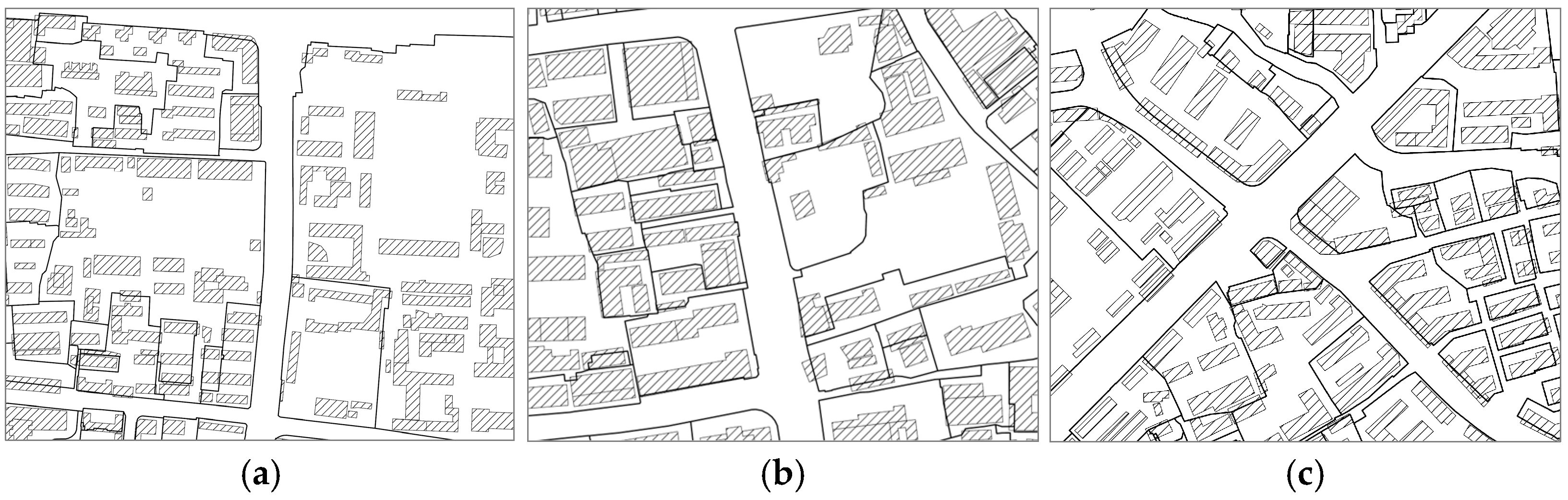
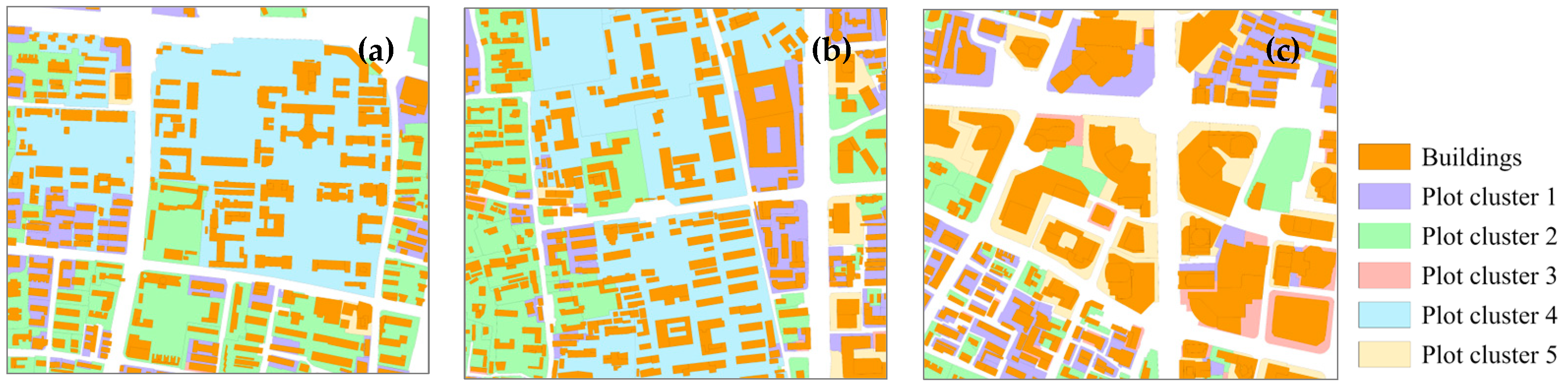
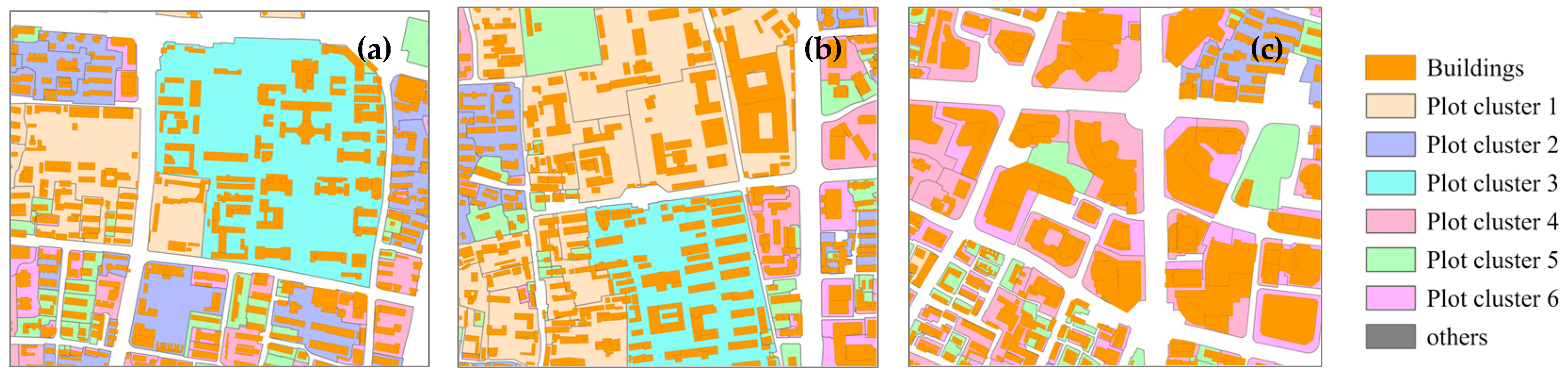
4.2.1. Morphological Types Identification

Among the plots that could be modeled as graphs, we randomly split the data into 70% for training and 30% for validation. After the training loss had converged, we concatenated the normalized plot-level attributes to each graph-level embedding, performed k-means clustering, and then mapped the cluster labels back onto the city map for spatial analysis (Figure 4). For plots that could form graphs, this procedure yielded five clusters once the embeddings and attributes were concatenated. Plots containing no more than two buildings were clustered directly by FAR, GSI, area, and perimeter; silhouette-guided k-means suggested two clusters in this subset. Taken together, the seven clusters are unevenly distributed: Cluster 6, characterized by low-FAR plots with only one or two buildings, encompasses 3647 parcels (40.6% of all plots) covering 4,644,257 m². In contrast, Cluster 3, featuring moderate-FAR but very large plots, includes only 16 parcels yet spans 4,543,404 m², with each parcel containing at least 29 buildings. Both the number of plots and the area share therefore vary markedly across clusters. When the seven cluster labels are visualized on the city map, it becomes evident that morphology-based classifications do not correspond neatly to geographic distributions within the walled city, revealing the spatial distribution of the identified morphological types.

Figure 5 visualizes how the seven clusters differ in four key morphological metrics: parcel area, building count, GSI, and FAR. Although overlap is visible, the box plots already reveal that certain metrics have separated the groups. Figure 6 therefore moves from aggregated statistics to spatial evidence: it zooms into three representative urban sectors and maps the cluster labels onto the actual urban fabric. By comparing the clusters in Figure 5 with the planform patterns in Figure 6, we can verify the proposed method indeed captures spatial relationship types more accurately. A closer examination of each cluster confirms these distinct differences (metrics of all clusters are presented in Appendix A,

Table A1. Basic metrics of plot clusters in Nanjing’s walled city.

Metrics	Cluster 1	Cluster 2	Cluster 3	Cluster 4	Cluster 5	Cluster 6	Cluster 7
plot_count	202	259	15	1113	1263	3647	2474
total_area	9,044,316	1,641,203	4,543,404	6,101,306	6,852,669	4,344,258	2,250,693
mean_area	44,773.84	6336.69	302,893.6	5481.857	5425.708	1191.187	909.7383
median_area	36,191.13	4865.828	215,958.1	4122.018	3633.609	839.7579	599.6674
max_area	149,108.6	28,247.99	941,229	29,456.58	34,180.04	93,661.29	28,865.74
plot_max_area	1243	6642	2282	2792	2364	4536	8001
min_area	10,096.85	676.7026	180,580.6	227.4779	130.8906	42.82825	19.28698
plot_min_area	8674	2259	244	8391	415	3005	1755
total_buildings	4793	1290	1781	6228	7025	4798	3129
mean_buildings	23.72772	4.980695	118.7333	5.595687	5.562154	1.315602	1.264753
median_buildings	20	4	105	4	4	1	1
max_buildings	91	32	427	31	32	2	2
plot_max_buildings	7612	7681	2282	6946	7393	7	14
min_buildings	3	3	29	3	3	1	1
plot_min_buildings	1637	33	1225	5	36	1	2
coverage_mean	0.27465	0.484504	0.193145	0.367458	0.418382	0.338197	0.64935
coverage_median	0.271831	0.469069	0.2342	0.360743	0.398814	0.352608	0.61968
coverage_max	0.630115	1.577616	0.28901	0.926781	1.124933	0.584816	1
coverage_min	0.022058	0.150293	0.04755	0.039009	0.048126	0.000442	0.247814
FAR_mean	1.730994	8.60342	1.238802	2.221596	2.456136	1.801078	3.693972
FAR_median	1.712884	7.429124	1.064944	2.143638	2.336872	1.763918	3.362612
FAR_max	5.564863	33.86183	4.514469	6.678434	6.262421	8.232607	46.52596
FAR_min	0.039021	3.248306	0.11144	0.039009	0.237339	0.001767	0.587176

). In Figure 6, although cluster 3 contains few plots, each of these plots accommodates a higher number of buildings compared to other clusters. However, its average GSI and FAR are the lowest, indicating that—even with many buildings and large land take—these plots are not built at a high density. The opposite holds for cluster 2, which contains few buildings and only a moderate average plot area but high average GSI and FAR signal-intensive development. Typical examples of cluster 2 are the university campus in the northeast of Figure 6a and the downtown commercial complex in the center of Figure 6c. Cluster 1 shows a classic mixed commercial–residential fabric; by contrast, cluster 4 consists of slab blocks in a single row, whereas cluster 5 exhibits more complex inter-building spatial relations owing to its irregular plot outlines. Clusters 6 and 7 are simple development plots whose classification is driven largely by overall building intensity.

4.2.2. Classification Strengthened by Building Relation Features

The incorporation of inter-building spatial relationships alongside building morphological features provides a more refined basis for typological classification. To verify the value of this approach, we constructed a Baseline 0 that clusters plots solely by their own morphology. Baseline 0 uses four indicators—area, perimeter, GSI, and FAR—as the clustering variables. Silhouette-driven k-means on these four metrics yielded five clusters across the walled city of Nanjing. Clusters 1 and 2 together hold 81.0% of the plots count but only 54.8% of the total area. Cluster 3, by contrast, contains only 2.5% of the plot count but 39.4% of the area, with mostly very large parcels. Because clustering is based only on plot attributes, those attributes dominate the partition. Measures such as GSI reflect building volume; compared with the Baseline 0, our approach captures inter-building spatial relations and therefore plays a more decisive role (Spatial distribution of Baseline 0 is presented in Appendix A, Figure A2).

Plotting the results in a Space Matrix diagram (Figure 7) makes the difference explicit. In the Baseline 0 clustering, each cluster occupies a well-defined wedge-shaped region, with the point distributions within each cluster forming compact groupings; FAR and GSI alone define the boundaries. In contrast, our results show significant overlap across identical FAR–GSI value ranges, with multiple clusters frequently appearing within what would traditionally be considered a single density category. Baseline 0 therefore classifies mainly by the density dyad—built floor area versus ground coverage—and overlooks morphological variation within a given FAR–GSI band. Our approach still separates plots within identical FAR and GSI values into multiple clusters. The algorithm clearly identifies clusters based on latent dimensional features that are not immediately visible in two-dimensional projections. These features include building distributions, building morphologies, and inter-building distances, which become apparent only when the high-dimensional GAT embeddings capture their complex relationships. For instance, within a similar FAR, tower-, slab- and composite-type plots are further distinguished. The color overlaps in the Space Matrix panel demonstrate that the new model has successfully introduced third- and fourth-dimensional shape information.

Figure 8 compares the results from both approaches in the same city sectors as Figure 6 to visualize the improved recognition of morphological patterns. The overall trends and broad types remain consistent, showing that both models capture the same direction of variation. For example, Figure 8a identifies school campuses, Figure 8b recognizes danwei compounds (work unit compounds characteristic of China’s socialist urban planning with enclosed collective living and working spaces), and Figure 8c detects major high-rise complexes. The small-scale, low-rise neighborhoods are uniformly colored, showing that the model correctly detects the “dense low-rise + narrow lane” graph structure, which is characterized by closely packed buildings of 1–3 stories arranged along narrow pedestrian pathways typical of traditional urban fabrics.

However, unlike the attribute-only baseline, our model gives decisive weight to inter-building spatial relations, enabling finer distinctions. In Figure 6a, an axial school campus is separated from adjacent living quarters, yet similar residential fabrics are consistently labeled in Figure 8a. In Figure 8b, the purple plots on the eastern side, though similar in GSI and area, were grouped into a single category by the baseline method. However, under our classification approach, these plots are classified as distinct types because of their different building relationship patterns (see eastern plots in Figure 6b). Similarly, in the lower-right corner of Figure 8c, plots with irregular shapes that were incorrectly grouped by the baseline method are properly classified when building form and spatial relationships are taken into account (see Figure 6c).

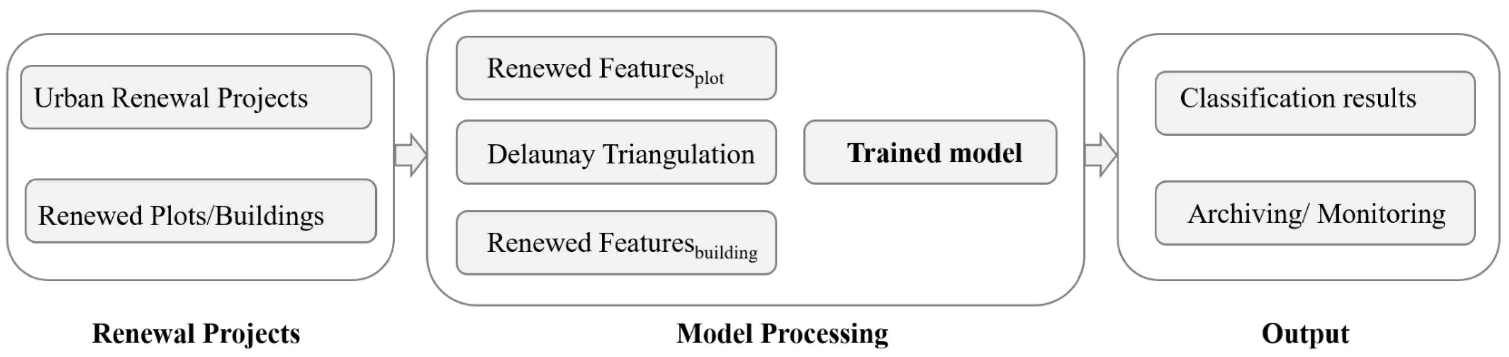
4.2.3. Urban Renewal Implications

The seven clusters possess distinct geometric and relational signatures—building count, orientation, and mutual arrangement (Figure 9)—which assist architects in understanding the urban fabric. Type 1 (median FAR around 1.7) consists of parallel slabs with occasional courtyard blocks and dense, uniform lanes, typical of 1980s–1990s worker housing. Type 2 (median FAR around 8.2) shows very high development intensity and falls in the high-FAR zone of the Space Matrix, representing mixed-use towers, offices, hotels, and complexes. Type 3 (median FAR around 1.3) covers universities, science parks, and old factories, usually with an auditorium or courtyard at the center. Type 4 (median FAR around 2.2) comprises widely spaced slab blocks, often serving as dormitories, hospitals, or research housing. Type 5 (median FAR around 2.5) mixes short slabs with interlocking courtyard blocks, common in older estates and resettlement areas. Type 6 contains one or two single-story to three-story buildings, typically petrol stations, corner supermarkets, warehouses, or small detached houses. Type 7 has the highest GSI (0.7) and an FAR of 3.7, marking landmark offices and five-star hotels; its extreme GSI is the key discriminator. The classification is therefore grounded in plot morphology, building form, and their spatial relations. These typological classifications are not completely aligned with functional uses but rather primarily reflect morphological characteristics. Each prototype depends not only on FAR/GSI but also on building count, shape, enclosure, and massing—all captured by the Delaunay–GAT convolutions.

Morphology-based classification can guide various urban renewal approaches in practical implementation. In practical renewal, Type 1 pinpoints plots suited to micro-renovation plus public-space upgrades; Type 2 locates high-capacity development nodes for FAR control and skyline studies; Type 3 guides zoning and phased reuse of industrial heritage; Type 4 supports green-belt redevelopment; Type 5 suggests pilot projects for neighborhood micro-circulation; Type 6 indicates strategic micro-interventions, such as pocket parks; and Type 7 serves as a baseline for skyline and daylight analysis. These seven plot archetypes thus carry practical value for urban regeneration. By introducing building relation classes alongside traditional functional categories, the typology provides a robust spatial data foundation for renewal strategies.

5. Discussion

5.1. Triple Loss Function Validation

Our method guides unsupervised learning and clustering through three essential elements of plot analysis. Compared to using only plot morphological features, our approach demonstrates more refined and accurate plot classification by incorporating both building morphology and inter-building spatial relations (see Section 4.2.2). To demonstrate the model’s ability to learn from both building morphology and spatial relation among buildings, we conducted ablation studies by either removing the link prediction loss (which guides inter-building spatial relations learning) or substantially reducing the proportion of mutual information loss on node features (which guides building morphology learning) in the GAT and then compared the clustering results. This analysis validates our method’s capability to capture comprehensive features.

For Baseline 1, we removed the link prediction loss from our triple-loss function, guiding GAT learning with only mutual information loss and regulation loss. When the model’s ability to learn the edge structure of the graph was disabled, it focused on learning the morphological features of each building node, aiming to minimize the distance between graph-level embeddings and node features at convergence. Although the computational graph of GAT inherently contains spatial structural features, meaning the converged graph-level embeddings still retain some latent structural characteristics, structural features were not explicitly optimized during learning. Through analysis, we found that Baseline 1 produced the same number of clusters as our full model (Spatial distribution is presented in Appendix A, Figure A3). This indicates that, similar to our model, Baseline 1 also learned multiple plot features through the GAT. However, there were differences in the specific category divisions. Since the focus was on learning building morphology, plots with similar building forms were classified together even when their spatial relationships differed. Conversely, plots with similar inter-building spatial relations but differences in building morphology were separated into different categories. For example, in Figure 10b, plots in the southeast that belong to the same category in our full model were divided into two categories due to inconsistencies in building morphology, and the strip-building plots on the west side of the southern compound were also divided into multiple categories.

For Baseline 2, we significantly reduced the proportion of mutual information loss from our triple loss function, guiding GAT learning primarily with link prediction loss and regulation loss. This disabled the model’s learning of building morphological features at the node level, focusing instead on the inter-building spatial relations to ensure that the graph-level embeddings captured edge features at convergence. The link prediction loss directed the model to bring the representations of positive node pairs (connected by edges) closer together while pushing apart negative node pairs (not connected by edges). Therefore, we anticipated that the learning results would emphasize graph connectivity while still incorporating some learning of building morphological features. Through analysis, we found that Baseline 2 produced six cluster types (the spatial distribution of Baseline 2 is presented in Appendix A, Figure A4). This indicates that learning based on structure identified some potential clustering patterns (compared to clustering results based solely on plot features), though the specific classifications differed from our full model. Because the focus was primarily on spatial structure learning, we observed that some plots with differences in building morphology were classified together due to high similarity in graph structure. Conversely, plots with similar building morphology but differences in structure were separated in the clustering. For example, in Figure 11b, the middle plots in the northern block were classified together with surrounding plots despite inconsistencies in building morphological features because their graph structural features were similar.

The purpose of our model design was to incorporate building morphology, inter-building spatial relations, and plot morphology as three essential aspects guiding unsupervised plot classification. Compared to learning only building morphological features or only building spatial relationship features, our triple loss function demonstrates the ability to effectively integrate all three aspects. Baselines 1 and 2 do not represent incorrect classifications, but rather, in the context of our method design aimed at fine-grained urban renewal practice, our full model better balances multiple aspects of features, thus providing a practice-oriented plot morphology classification.

5.2. Theoretical Implications

Our graph-based approach delivers computational insights into plot–building relations, reconciling divergent theoretical traditions within urban morphology. By treating buildings not as isolated objects but as spatially interrelated components embedded in their plots, the GAT model simultaneously captures the historical evolution stressed by the Conzen school and the building typology foregrounded in the Italian tradition. It thus bridges a long-standing theoretical gap: while Conzen and Whitehand established the plot as the fundamental morphological unit and Caniggia and Maffei emphasized building types as spatial modules, both traditions offered opportunities for developing quantitative tools to analyze how collective spatial relations shape plot characteristics. Our framework operationalizes this relation by encoding buildings as feature-rich nodes in a plot-defined graph, thereby providing a computational realization that unifies these complementary perspectives. The introduction of graph theory allows the hierarchical morphological scales—building, plot, block, and urban fabric—to be expressed through interlinked graph features, establishing a foundation for further analysis. Taken together, the synthesis demonstrates how graph theory can formalize morphological concepts previously described only qualitatively, enabling researchers to test and refine classical typological theories with large-scale quantitative methods.

Our three-aspect plot analysis approach combines building morphology, inter-building spatial relations, and plot attributes; the corresponding triple loss function design in the graph attention network guides the model to learn all three dimensions. The method makes unsupervised learning possible while preserving interpretability—a crucial balance for morphological analysis that must remain intelligible to planners—and therefore represents a methodological innovation. In doing so, it advances the theoretical agenda of plot-based urbanism, which positions the plot as a key lever for sustainable urban renewal [2]. Grounded in the fine-grained needs of renewal practice, we construct a detailed plot typology that implements this idea. By identifying seven distinct plot types in Nanjing, capturing variations in both plot metrics and internal building configurations, our approach provides the differentiated classification required for resilient urban form [6]. Each type points to a specific renewal strategy: Type 1 (parallel slabs with lanes) suggests incremental upgrading; Type 2 (high-intensity development) signals sites where FAR control is critical; and Types 3–7 offer targeted urban renewal templates ranging from heritage conservation to infill development. This direct link between theoretical classification and practical application illustrates how computational methods can extend morphological theory from analysis to an actionable planning framework for complex urban environments.

5.3. From Genesis to Application

5.3.1. Historical Genesis of the Seven Types

The seven plot types identified by our model did not emerge randomly; each reflects a distinct trajectory in Nanjing’s land use history and thus points to a specific renewal option. Precisely because these seven types grew out of different historical layers, urban designers can leverage their spatial features when reusing parcels and guiding renewal. In practice, recognizing which combination of plot and building belongs to which type allows designers to choose an appropriate intervention.

For type 1, these parallel slabs and occasional courtyard blocks can be traced back to the danwei system, when large state employers received land free of charge and followed uniform building codes. Most structures are now aging, and because parcel boundaries and road widths are fixed, small-scale refurbishment and structural reinforcement can produce the best results. Type 2 comprises the high-FAR tower-and-podium complexes that have risen since the 1990s. Their intense morphology calls for maintenance, skyline control, view-corridor protection, and podium permeability studies rather than demolition. As the institutional courtyard compound, Type 3’s regular rows of buildings around a central hall reflect planning for campuses and factories. Many such parcels have already been converted into science parks, and—in suitable locations—can also be opened as public parks. Type 4 shows fewer but denser slab blocks on relatively small plots. This pattern is especially common when a compact parcel must still accommodate relatively intensive building volume. These have become a priority for contemporary renewal, where measures such as rooftop solar retrofits improve energy efficiency without displacing residents. Type 5 consists of short slab buildings arranged on irregular parcels produced during village-in-city clearance. In the early stage of urban renewal, most relocated households were resettled in such estates. These neighborhoods feature active ground-floor commerce. Focusing on retail-quality upgrades and sanitation improvements is enough to keep them in good status. Type 6 represents the classical one-plot-one-building pattern common in Nanjing’s early modern expansion; because most parcels remain privately owned, renewal is steered mainly by urban design guidelines. Finally, Type 7 contains landmark high-rise parcels with isolated slender towers built to maximize branding in the commercial era. These parcels are usually quite recent. At present, they often require interior refurbishment to attract new office or hotel tenants and sustain vitality.

Several urban renewal architects have confirmed that classifying Nanjing’s plots into seven types is both reasonable and useful, helping architects sort thousands of plots efficiently and avoiding the randomness of purely manual judgment.

5.3.2. Application Workflow in Design Practice

When the model outputs the seven plot types, it simultaneously stores the converged weights. A 7:3 train–validation split guarantees robustness. Practitioners need not master every technical detail. They need only grasp the fundamental logic. That is, instead of judging plots by only morphological metrics, it is more useful to fuse building morphology, spatial relations, and parcel attributes. Because the fixed weights already encode Nanjing’s complex features, designers simply feed in updated plot and building data to obtain the corresponding type and guide renewal precisely.

Concretely, the steps are as follows: once a designer completes a scheme, the parcel’s numerical attributes—building shapes, spatial relations, parcel metrics—can be directly exported. A short script reads the new data, constructs the graph, and passes it through the fixed model once to extract a graph embedding (with trained weights). K-means then assigns the plot to the cluster whose centroid the embedding belongs to (Figure 12). In other words, the designer does not have to re-run the training process. Supplying the updated CAD file and using the pre-trained weights is adequate to produce the type label, greatly streamlining future renewal work.

5.4. Research Limitations

Qualitative, experience-based analyses have long been employed to classify urban plots according to practical needs. However, in the historic cores of complex Global South cities, plot types, distributions, and attributes are so intricate that qualitative methods become inefficient when faced with large datasets. Moreover, because such approaches depend on the expertise of traditional architects and practitioners, the resulting typologies are subject to personal value judgments. Conversely, conventional quantitative techniques—clustering plots by morphological and building metrics—can indeed deliver stable city-wide plot classifications. However, as research and renewal practice for historic districts reach a finer-grained stage, plot descriptors must capture not only building intensity and building count but also the spatial relations among buildings. Hence, an unsupervised plot classification framework that automatically derives plot types from plot and building data can boost both efficiency and accuracy while objectively incorporating building relations through graph structures and thereby combining the strengths of qualitative and quantitative approaches. Traditional classifications remain useful for tasks such as index regulation and FAR zoning that guide construction through development intensity controls. In contrast, the present method, which separates plots with similar indices but distinct morphologies, can underpin more precise urban-renewal interventions. Nevertheless, several limitations emerge when applying this morphology-oriented approach:

Data availability. Building data are comparatively easy to obtain from numerous repositories, whereas plot data are difficult to collect because they hinge on land ownership records. This study focused on methodological soundness and validated the approach with Nanjing data. For higher-precision results or a complete software package that reads data from multiple cities and outputs plot types, a much larger input of plot information will be required.

Algorithmic and model explainability. The triple-loss design combines spatial structure with plot morphology and produces interpretable outcomes; nevertheless, the constant structural patterns learned by the network—and their links to the input features—remain opaque. In addition, Delaunay triangulations, Voronoi graphs, and weighted fully connected graphs capture connectivity with differing sparsity and structural emphases; these differences alter the feature signals that the GAT receives and can, in turn, influence the clustering. Whether a sparser minimum-spanning tree graph or a hybrid fusing several graph types would yield conclusions better aligned with the research goals warrants further investigation.

Social perspective. Parcel evolution is the result of long-term historical processes—including ownership, modes of use, and the form and size of buildings—all closely tied to everyday living. Consequently, renewal strategies that take plot morphology as a starting point must integrate human factors. Although this study still concentrates on plots and buildings, future work will extend the framework to incorporate social variables.

To address these limitations, future work will explore the following:

Integrating richer data sources. Beyond the morphological variables considered here, introducing accessibility and functional data at the plot level could further refine the clusters and produce a more robust and generalizable framework.

Translating classifications into practice. With accessibility data in place, we will examine how morphology-accessibility clusters correlate with plot functions, thereby informing the prediction, design, and renewal of plot uses and forms in concrete urban-update projects.

Algorithmic optimization. The current feature set is still extensive and computationally demanding; forthcoming work will test the marginal contribution of each morphological indicator, retain only the most informative features, and thus achieve classification with fewer variables and lower computational cost. We will also assign learnable weights to different graph types and let the convolutional network optimize their contribution automatically so that building relations are captured with greater precision.

People-centered considerations. When implementing renewal strategies based on plot classification results, it is essential to further account for human needs. For instance, strategies may differ significantly depending on the function of the plot. In future work, we will incorporate user needs and community characteristics to refine and adapt plot-specific renewal strategies accordingly.

6. Conclusions

This research addressed the challenge of accurately classifying urban plots in complex built environments where conventional metrics fail to capture intricate spatial relationships among buildings, with the aim of enabling more refined urban renewal practices. By developing a graph-based representation learning approach, we sought to improve plot classification by explicitly modeling inter-building spatial relationships while maintaining morphological interpretability. Our key findings demonstrate that Graph Attention Networks can effectively learn latent patterns in both building morphology and spatial topology, producing meaningful plot classifications that extend beyond what conventional metric-based approaches capture.

Theoretically, this work contributes to urban morphology research by bridging quantitative and qualitative approaches. The graph-based representation offers a computational framework that aligns with morphological theories emphasizing relational aspects of urban form, while the resulting typology maintains architectural and spatial interpretability essential for planning practice. By modeling plots as graphs and buildings as nodes, our approach captures the hierarchical nature of urban form that traditional morphological schools have long emphasized.

Building on this theoretical contribution, this study also advances land use research. It offers a deep learning methodology that evaluates plot typologies by extending traditional indices into a three-dimensional set—plot metrics, building metrics, and spatial-relation metrics. Requiring only two common inputs (plot and building data), the framework can be transferred to other complex urban fabrics: each city can retrain the model on its own data and obtain its own typology system. Once converged, the model no longer needs retraining; updating the input data is sufficient to refresh plot types, enabling real-time monitoring. The work provides both morphological insight and a practical tool for land use management.

In conclusion, the graph-based approach presented in this study demonstrates that explicitly modeling spatial relationships among buildings significantly enhances our ability to classify urban plots, particularly in complex environments characteristic of many Global South cities. By capturing both metric and relational aspects of urban form, our framework provides both researchers and practitioners with a more precise tool for understanding urban morphology and guiding targeted interventions for sustainable urban regeneration.

References

1. Conzen, M.R.G. Alnwick, Northumberland: A Study in Town-Plan Analysis. Trans. Pap. (Inst. Br. Geogr.) 1960, iii–122. [Google Scholar] [CrossRef]
2. Porta, S.; Romice, O. Plot-Based Urbanism: Towards Time-Consciousness in Place-Making; University of Strathclyde: Glasgow, UK, 2010; pp. 1–39. [Google Scholar]
3. Kropf, K. Aspects of Urban Form. Urban Morphol. 2009, 13, 105–120. [Google Scholar] [CrossRef]
4. Kropf, K. Ambiguity in the Definition of Built Form. JUM 2013, 18, 41–57. [Google Scholar] [CrossRef]
5. Barbour, G.; Romice, O.; Porta, S. Sustainable Plot-Based Urban Regeneration and Traditional Master Planning Practice in Glasgow. Open House Int. 2016, 41, 15–22. [Google Scholar] [CrossRef]
6. Feliciotti, A.; Romice, O.; Porta, S. Urban Regeneration, Masterplans and Resilience: The Case of Gorbals, Glasgow. Urban Morphol. 2017, 21, 61–79. [Google Scholar] [CrossRef]
7. Caniggia, G.; Maffei, G.L. Composizione Architettonica e Tipologia Edilizia; FLORE: Marsilio, Venezia, 1979; Volume 1. [Google Scholar]
8. Conzen, M.R.G.; Whitehand, J.W.R. The Urban Landscape: Historical Development and Management; Academic Press: Cambridge, MA, USA, 1981. [Google Scholar]
9. Caniggia, G.; Maffei, G.L. Architectural Composition and Building Typology: Interpreting Basic Building; Alinea Editrice: Firenze, Italy, 2001; Volume 176. [Google Scholar]
10. Bobkova, E.; Berghauser Pont, M.; Marcus, L. Towards Analytical Typologies of Plot Systems: Quantitative Profile of Five European Cities. Environ. Plan. B Urban Anal. City Sci. 2021, 48, 604–620. [Google Scholar] [CrossRef]
11. Dovey, K.; van Oostrum, M.; Chatterjee, I.; Shafique, T. Towards a Morphogenesis of Informal Settlements. Habitat Int. 2020, 104, 102240. [Google Scholar] [CrossRef]
12. Simone, A. Cities of the Global South. Annu. Rev. Sociol. 2020, 46, 603–622. [Google Scholar] [CrossRef]
13. Batty, M. The New Science of Cities; MIT Press: Cambridge, MA, USA, 2013; ISBN 978-0-262-01952-1. [Google Scholar]
14. Ghosh, S.; Mallick, A.; Chowdhury, A.; De Sarkar, K.; Mukherjee, J. Graph Theory Applications for Advanced Geospatial Modelling and Decision-Making. Appl. Geomat. 2024, 16, 799–812. [Google Scholar] [CrossRef]
15. Marshall, S.; Gil, J.; Kropf, K.; Tomko, M.; Figueiredo, L. Street Network Studies: From Networks to Models and Their Representations. Netw. Spat. Econ. 2018, 18, 735–749. [Google Scholar] [CrossRef]
16. Wang, J.; Biljecki, F. Unsupervised Machine Learning in Urban Studies: A Systematic Review of Applications. Cities 2022, 129, 103925. [Google Scholar] [CrossRef]
17. Panerai, P.; Castex, J.; Depaule, J.-C.; Samuels, I. Urban Forms: The Death and Life of the Urban Block; Routledge: London, UK, 2004; ISBN 978-0-7506-5607-8. [Google Scholar]
18. Kropf, K. Plots, Property and Behaviour. JUM 2017, 22, 5–14. [Google Scholar] [CrossRef]
19. Attilio, P. After Amnesia. Learning from the Islamic Mediterranean; Icar: Bari, Italy, 2007; ISBN 9788895006031. [Google Scholar]
20. Song, Y.; Zhang, Y.; Han, D. Deciphering Built Form Complexity of Chinese Cities through Plot Recognition: A Case Study of Nanjing, China. Front. Archit. Res. 2022, 11, 795–805. [Google Scholar] [CrossRef]
21. Whitehand, J.W.R.; Gu, K.; Conzen, M.P.; Whitehand, S.M. The Typological Process and the Morphological Period: A Cross-Cultural Assessment. Environ. Plann. B Plann. Des. 2014, 41, 512–533. [Google Scholar] [CrossRef]
22. Elzeni, M.; Elmokadem, A.; Badawy, N.M. Classification of Urban Morphology Indicators towards Urban Generation. Port-Said Eng. Res. J. 2022, 26, 43–56. [Google Scholar] [CrossRef]
23. Hermosilla, T.; Ruiz, L.A.; Recio, J.A.; Cambra-López, M. Assessing Contextual Descriptive Features for Plot-Based Classification of Urban Areas. Landsc. Urban Plan. 2012, 106, 124–137. [Google Scholar] [CrossRef]
24. Berghauser Pont, M.; Marcus, L. Innovations in Measuring Density: From Area and Location Density to Accessible and Perceived Density. Nat. Astron. 2014, 26, 2–9. [Google Scholar]
25. Berghauser Pont, M.; Haupt, P.A. Spacematrix: Space, Density and Urban Form; TU Delft OPEN: Municipality of Norrköping, Sweden, 2023. [Google Scholar]
26. Marcus, L. Spatial Capital. A Proposal for an Extension of Space Syntax into a More General Urban Morphology. J. Space Syntax. 2010, 1, 30–40. [Google Scholar]
27. Marcus, L.; Bobkova, E. Spatial Configuration of Plot Systems and Urban Diversity: Empirical Support for a Differentiation Variable in Spatial Morphology. In Proceedings of the 12th Space Syntax Symposium, Beijing, China, 8–13 July 2019; Volume 494, p. 1. [Google Scholar]
28. Scoppa, M.D.; Peponis, J. Distributed Attraction: The Effects of Street Network Connectivity upon the Distribution of Retail Frontage in the City of Buenos Aires. Environ. Plann. B Plann. Des. 2015, 42, 354–378. [Google Scholar] [CrossRef]
29. Porta, S.; Romice, O.; Strano, E.; Venerandi, A.; Morello, E.; Viana, M.; Da Fontoura Costa, L. Plot-Based Urbanism and Urban Morphometrics: Measuring the Evolution of Blocks, Street Fronts and Plots in Cities. 2011. Available online: https://strathprints.strath.ac.uk/35639/ (accessed on 13 July 2025).
30. Bobkova, E. Towards a Theory of Natural Occupation: Developing Theoretical, Methodological and Empirical Support for the Relation between Plot Systems and Urban Processes. Ph.D. Thesis, Chalmers Tekniska Hogskola, Gothenburg, Sweden, 2019. [Google Scholar]
31. Ye, Y.; van Nes, A. Quantitative Tools in Urban Morphology: Combining Space Syntax, Spacematrix and Mixed-Use Index in a GIS Framework. Urban Morphol. 2014, 18, 97–118. [Google Scholar] [CrossRef]
32. Marshall, S. An Area Structure Approach to Morphological Representation and Analysis. JUM 2014, 19, 117–134. [Google Scholar] [CrossRef]
33. Braun, A.; Warth, G.; Bachofer, F.; Schultz, M.; Hochschild, V. Mapping Urban Structure Types Based on Remote Sensing Data—A Universal and Adaptable Framework for Spatial Analyses of Cities. Land 2023, 12, 1885. [Google Scholar] [CrossRef]
34. Li, R.; Sun, T.; Ghaffarian, S.; Tsamados, M.; Ni, G. GLAMOUR: GLobAl Building MOrphology Dataset for URban Hydroclimate Modelling. Sci. Data 2024, 11, 618. [Google Scholar] [CrossRef] [PubMed]
35. Vanderhaegen, S.; Canters, F. Mapping Urban Form and Function at City Block Level Using Spatial Metrics. Landsc. Urban Plan. 2017, 167, 399–409. [Google Scholar] [CrossRef]
36. Usui, H. Statistical Distribution of Building Lot Depth: Theoretical and Empirical Investigation of Downtown Districts in Tokyo. Environ. Plan. B Urban Anal. City Sci. 2019, 46, 1499–1516. [Google Scholar] [CrossRef]
37. Fleischmann, M.; Feliciotti, A.; Romice, O.; Porta, S. Methodological Foundation of a Numerical Taxonomy of Urban Form. Environ. Plan. B Urban Anal. City Sci. 2022, 49, 1283–1299. [Google Scholar] [CrossRef]
38. Karimi, F.; Sultana, S.; Shirzadi Babakan, A.; Suthaharan, S. An Enhanced Support Vector Machine Model for Urban Expansion Prediction. Comput. Environ. Urban Syst. 2019, 75, 61–75. [Google Scholar] [CrossRef]
39. Ruiz Hernandez, I.E.; Shi, W. A Random Forests Classification Method for Urban Land-Use Mapping Integrating Spatial Metrics and Texture Analysis. Int. J. Remote Sens. 2018, 39, 1175–1198. [Google Scholar] [CrossRef]
40. Liu, S.; Liu, R.; Tan, N. A Spatial Improved-kNN-Based Flood Inundation Risk Framework for Urban Tourism under Two Rainfall Scenarios. Sustainability 2021, 13, 2859. [Google Scholar] [CrossRef]
41. Jun, M.-J. A Comparison of a Gradient Boosting Decision Tree, Random Forests, and Artificial Neural Networks to Model Urban Land Use Changes: The Case of the Seoul Metropolitan Area. Int. J. Geogr. Inf. Sci. 2021, 35, 2149–2167. [Google Scholar] [CrossRef]
42. Zhang, P.; Ghosh, D.; Park, S. Spatial Measures and Methods in Sustainable Urban Morphology: A Systematic Review. Landsc. Urban Plan. 2023, 237, 104776. [Google Scholar] [CrossRef]
43. Chen, C.-Y.; Koch, F.; Reicher, C. Developing a Two-Level Machine-Learning Approach for Classifying Urban Form for an East Asian Mega-City. Environ. Plan. B 2024, 51, 854–869. [Google Scholar] [CrossRef]
44. Batty, M. Cities as Complex Systems: Scaling, Interaction, Networks, Dynamics and Urban Morphologies. In Encyclopedia of Complexity and Systems Science; Meyers, R.A., Ed.; Springer: New York, NY, USA, 2009; pp. 1041–1071. ISBN 978-0-387-30440-3. [Google Scholar]
45. Caruso, G.; Hilal, M.; Thomas, I. Measuring Urban Forms from Inter-Building Distances: Combining MST Graphs with a Local Index of Spatial Association. Landsc. Urban Plan. 2017, 163, 80–89. [Google Scholar] [CrossRef]
46. Fan, C.; Yang, Y.; Mostafavi, A. Neural Embeddings of Urban Big Data Reveal Spatial Structures in Cities. Humanit. Soc. Sci. Commun. 2024, 11, 409. [Google Scholar] [CrossRef]
47. Lei, B.; Liu, P.; Milojevic-Dupont, N.; Biljecki, F. Predicting Building Characteristics at Urban Scale Using Graph Neural Networks and Street-Level Context. Comput. Environ. Urban Syst. 2024, 111, 102129. [Google Scholar] [CrossRef]
48. Chen, D.; Feng, Y.; Li, X.; Qu, M.; Luo, P.; Meng, L. Interpreting Core Forms of Urban Morphology Linked to Urban Functions with Explainable Graph Neural Network. Comput. Environ. Urban Syst. 2025, 118, 102267. [Google Scholar] [CrossRef]
49. You, Y.; Chen, T.; Sui, Y.; Chen, T.; Wang, Z.; Shen, Y. Graph Contrastive Learning with Augmentations. Advances in neural information Process. Systems. arXiv 2020, arXiv:2010.13902. [Google Scholar]
50. Veličković, P.; Cucurull, G.; Casanova, A.; Romero, A.; Liò, P.; Bengio, Y. Graph Attention Networks. arXiv 2018, arXiv:1710.10903. [Google Scholar]
51. Wang, G.; Ying, R.; Huang, J.; Leskovec, J. Improving Graph Attention Networks with Large Margin-Based Constraints. arXiv 2019, arXiv:1910.11945. [Google Scholar] [CrossRef]
52. Zhu, Y.; Xu, Y.; Liu, Q.; Wu, S. An Empirical Study of Graph Contrastive Learning. arXiv 2021, arXiv:2109.01116. [Google Scholar] [CrossRef]
53. Fang, L.; Kou, Z.; Yang, Y.; Li, T. Representing Spatial Data with Graph Contrastive Learning. Remote Sens. 2023, 15, 880. [Google Scholar] [CrossRef]
54. Lelo, K. Analysing Spatial Relationships through the Urban Cadastre of Nineteenth-Century Rome. Urban Hist. 2020, 47, 467–487. [Google Scholar] [CrossRef]
55. Aurenhammer, F. Voronoi Diagrams—A Survey of a Fundamental Geometric Data Structure. ACM Comput. Surv. 1991, 23, 345–405. [Google Scholar] [CrossRef]
56. Lee, D.T.; Schachter, B.J. Two Algorithms for Constructing a Delaunay Triangulation. Int. J. Comput. Inf. Sci. 1980, 9, 219–242. [Google Scholar] [CrossRef]
57. Li, W.; Goodchild, M.F.; Church, R. An Efficient Measure of Compactness for Two-Dimensional Shapes and Its Application in Regionalization Problems. Int. J. Geogr. Inf. Sci. 2013, 27, 1227–1250. [Google Scholar] [CrossRef]
58. Basaraner, M.; Cetinkaya, S. Performance of Shape Indices and Classification Schemes for Characterising Perceptual Shape Complexity of Building Footprints in GIS. Int. J. Geogr. Inf. Sci. 2017, 31, 1952–1977. [Google Scholar] [CrossRef]
59. Gibbs, J.P. Urban Research Methods. In Van Nostrand Series in Sociology; University of Michigan: Ann Arbor, MI, USA, 1961. [Google Scholar]
60. Sun, F.-Y.; Hoffmann, J.; Verma, V.; Tang, J. InfoGraph: Unsupervised and Semi-Supervised Graph-Level Representation Learning via Mutual Information Maximization. arXiv 2020, arXiv:1908.01000. [Google Scholar]
61. Veličković, P.; Fedus, W.; Hamilton, W.L.; Liò, P.; Bengio, Y.; Hjelm, R.D. Deep Graph Infomax. arXiv 2018, arXiv:1809.10341. [Google Scholar] [CrossRef]
62. Grover, A.; Leskovec, J. Node2vec: Scalable Feature Learning for Networks. In Proceedings of the 22nd ACM SIGKDD International Conference on Knowledge Discovery and Data Mining, San Francisco, CA, USA, 13 August 2016; pp. 855–864. [Google Scholar]
63. Liu, P.; Neppl, M.; Dong, W. Smart Plot Division: Generating a Plot-Based Strategy for the Restoration of the Old South Historic Urban Area in Nanjing. Urban Des. Int. 2020, 25, 357–376. [Google Scholar] [CrossRef]
64. Caldeira, T.P. Peripheral Urbanization: Autoconstruction, Transversal Logics, and Politics in Cities of the Global South. Environ. Plan. D 2017, 35, 3–20. [Google Scholar] [CrossRef]
Figure 1. Complex plot–building relationships in Nanjing’s walled city: (a) danwei compounds and row housing with buildings spanning across multiple plots; (b) contrasting dense row layouts and sparse building arrangements; (c) diverse building morphologies and densities within plots. Source: authors, generated from the 2016 Nanjing dataset.
Land 14 01469 g001
Figure 2. Framework of the graph-based plot clustering methodology with three processing stages. Source: authors.
Land 14 01469 g002
Figure 3. Graph construction process: (a) original plot with buildings; (b) corresponding graph representation with buildings as nodes connected by Delaunay triangulation edges. Source: authors, generated from the 2016 Nanjing dataset.
Land 14 01469 g003
Figure 4. Spatial distribution of the seven plot morphology clusters across Nanjing’s walled city. Source: authors, generated from the 2016 Nanjing dataset.
Land 14 01469 g004
Figure 5. Distribution of key morphological indicators across the seven clusters: area, building count, GSI, and FAR. Source: authors, generated from the 2016 Nanjing dataset.
Land 14 01469 g005
Figure 6. Close-up views of plot classification results in three representative sectors: (a) educational and residential areas; (b) mixed-use neighborhood; (c) commercial district. Source: authors, generated from the 2016 Nanjing dataset.
Land 14 01469 g006
Figure 7. Comparison of plot distribution in Space Matrix diagram: (left) Baseline 0 clustering based only on plot metrics; (right) proposed method incorporating inter-building spatial relations. Source: authors, generated from the 2016 Nanjing dataset.
Land 14 01469 g007
Figure 8. Close-up views of the Baseline 0 clustering results (plot metrics only) in the same three sectors as Figure 6: (a) educational and residential areas; (b) mixed-use neighborhood; (c) commercial district. Source: authors, generated from the 2016 Nanjing dataset.
Land 14 01469 g008
Figure 9. Schematic representation of the seven morphological prototypes identified through the graph-based classification. Source: authors.
Land 14 01469 g009
Figure 10. Close-up views of clustering results from Baseline 1 (without link prediction loss) in the same sectors as Figure 6: (a) educational and residential areas; (b) mixed-use neighborhood; (c) commercial district. Source: authors, generated from the 2016 Nanjing dataset.
Land 14 01469 g010
Figure 11. Close-up views of clustering results from Baseline 2 (reduced mutual information loss) in the same sectors as Figure 6: (a) educational and residential areas; (b) mixed-use neighborhood; (c) commercial district. Source: authors, generated from the 2016 Nanjing dataset.
Land 14 01469 g011
Figure 12. Workflow for applying plot classification in urban renewal design. Source: authors.
Land 14 01469 g012