Article

Application of Semi-Supervised Clustering with Membership Information and Deep Learning in Landslide Susceptibility Assessment

1
Chongqing Jinfo Mountain Karst Ecosystem National Observation and Research Station, School of Geographical Sciences, Southwest University, Chongqing 400715, China
2
Chongqing Engineering Research Center for Remote Sensing Big Data Application, Southwest University, Chongqing 400715, China
3
State Key Laboratory of Cryospheric Science and Frozen Soil Engineering, Key Laboratory of Remote Sensing of Gansu Province, Heihe Remote Sensing Experimental Research Station, Northwest Institute of Eco-Environment and Resources, Chinese Academy of Sciences, Lanzhou 730000, China
*
Author to whom correspondence should be addressed.
Land 2025, 14(7), 1472; https://doi.org/10.3390/land14071472
Submission received: 4 June 2025 / Revised: 12 July 2025 / Accepted: 13 July 2025 / Published: 15 July 2025

Abstract

Landslide susceptibility assessment (LSA) plays a crucial role in disaster prevention and mitigation. Traditional random selection of non-landslide samples (labeled as 0) suffers from poor representativeness and high randomness, which may include potential landslide areas and affect the accuracy of LSA. To address this issue, this study proposes a novel Landslide Susceptibility Index–based Semi-supervised Fuzzy C-Means (LSI-SFCM) sampling strategy combining membership degrees. It utilizes landslide and unlabeled samples to map landslide membership degree via Semi-supervised Fuzzy C-Means (SFCM). Non-landslide samples are selected from low-membership regions and assigned membership values as labels. This study developed three models for LSA—Convolutional Neural Network (CNN), U-Net, and Support Vector Machine (SVM), and compared three negative sample sampling strategies: Random Sampling (RS), SFCM (samples labeled 0), and LSI-SFCM. The results demonstrate that the LSI-SFCM effectively enhances the representativeness and diversity of negative samples, improving the predictive performance and classification reliability. Deep learning models using LSI-SFCM performed with superior predictive capability. The CNN model achieved an area under the receiver operating characteristic curve (AUC) of 95.52% and a prediction rate curve value of 0.859. Furthermore, compared with the traditional unsupervised fuzzy C-means (FCM) clustering, SFCM produced a more reasonable distribution of landslide membership degrees, better reflecting the distinction between landslides and non-landslides. This approach enhances the reliability of LSA and provides a scientific basis for disaster prevention and mitigation authorities.

1. Introduction

Landslides are geological phenomena in which surface materials or rock masses move downslope under the influence of gravity. They typically occur on steep slopes or at the base of mountains, triggered by natural factors like rising groundwater levels, earthquakes, and rainfall [1], as well as human activities like overdevelopment, excavation, or irrational land use [2]. Landslides present significant threats to human life, infrastructure, and settlements [3], making timely assessment and prediction crucial for early risk warning [4], land-use planning [5], and social stability. Early susceptibility assessments primarily employed qualitative methods such as field surveys, manual mapping, and expert judgment based on engineering and geomechanical insights [6]. While sometimes effective, these approaches are inherently subjective, time-consuming, and labor-intensive. Consequently, enhancing efficiency and objectivity in landslide susceptibility assessment (LSA) has become a central aim in current disaster risk reduction research.
With the rapid advancements in deep learning and remote sensing, data-driven models have been increasingly applied to LSA [7]. Machine learning algorithms, such as support vector machines (SVMs) [8], random forests (RFs) [9], multilayer perceptrons [10], and artificial neural networks [11], have been widely used for natural disaster assessments. These models capture nonlinear relationships between triggering factors and landslide susceptibility, reduce overfitting, and achieve high prediction accuracy [2]. For instance, Xiao et al. combined RF and SHAP (SHapley Additive exPlanations) to establish an interpretable landslide susceptibility model [12]. Khuc et al. evaluated susceptibility using RF, gradient boosting, and SVM [13]. However, traditional machine learning algorithms often struggle to extract high-level representative features, capture complex nonlinear patterns, and efficiently process large-scale datasets [14]. In response, deep learning algorithms, especially convolutional neural networks (CNNs), are gradually being applied in disaster assessment [15,16,17]. The data-driven models are built by incorporating various independent triggering factors as input features and training on labeled landslide and non-landslide samples [18]. However, the performance of these data-driven models depends heavily on the quality and representativeness of both landslide and non-landslide samples, especially the latter, which can introduce uncertainty into the modeling process [19].
Samples form the foundation of landslide susceptibility modeling. Traditional datasets typically consist of positive and negative samples. Positive samples (labeled as 1) are usually obtained from historical landslide inventories, remote sensing interpretation, or field investigations. In contrast, the selection of negative samples (labeled as 0) is often characterized by subjectivity, randomness, and non-uniform distribution [20]. Common selection methods include random sampling [21], buffer exclusion around known landslides [22], low-slope filtering [23], and semi-supervised methods [24]. For example, Dou et al. used buffer zones and an information model for negative sample selection [25], but the choice of buffer distance remains subjective. Wang et al. selected negative samples from low-slope areas [26], which may neglect other critical factors contributing to landslide occurrence. Huang et al. chose negative samples from initially low-susceptibility zones [10], though their optimization strategy fails to fully capture the characteristics of non-landslide areas. Liu et al. applied unsupervised clustering to identify non-landslide samples from low-susceptibility regions [27]. Although the clustering approach reduces human intervention, it relies solely on inter-sample similarity and does not incorporate prior landslide knowledge, leading to uncertainties in the initial classification. Moreover, most existing studies assign a fixed label of 0 to all non-landslide samples, treating them as entirely “risk-free” regions [28,29]. In reality, however, these areas typically have a lower probability of landslide occurrence rather than being completely risk-free. While this simplification facilitates the modeling process, it overlooks the continuous nature of potential risk levels. This approach tends to mask the internal risk gradient within the samples, resulting in underrepresentation of negative sample features during model training and ultimately compromising prediction accuracy and practical reliability.
Therefore, this study proposes a semi-supervised clustering sampling strategy incorporating membership information to obtain more accurate non-landslide samples and enrich sample features. Semi-supervised clustering (SSC) is a technique that combines semi-supervised learning with clustering algorithms and has emerged as a new research direction in the field of machine learning in recent years [30]. Unlike unsupervised clustering, SSC integrates unlabeled and partially labeled data to guide the clustering process, thereby improving clustering accuracy [31]. Semi-supervised fuzzy C-means clustering (SFCM), a type of SSC, introduces membership degrees to effectively handle the uncertainty in sample class assignments. By mining the latent spatial structure of unlabeled samples and incorporating limited labeled landslide data to guide the clustering, SFCM yields reasonable clustering results and corresponding landslide membership degrees [32]. These membership values can be used to represent the initial Landslide Susceptibility Index (LSI). Based on this, a novel Landslide Susceptibility Index–based Semi-supervised Fuzzy C-Means (LSI-SFCM) sampling strategy was proposed. The LSI-SFCM sampling strategy selects non-landslide samples from low-membership regions and assigns the membership values as their labels, thereby enhancing the diversity of non-landslide samples.
To validate the effectiveness of the proposed method, this study takes Ya’an City, Sichuan Province, as a case study. Three negative sample sampling strategies—LSI-SFCM, semi-supervised clustering with labels set to 0 (SFCM), and random sampling (RS)—are used to construct U-Net, CNN, and SVM models. The model performance and spatial distribution characteristics of landslide susceptibility under different strategies are compared and analyzed.

2. Study Area

Ya’an City, located in the western Sichuan Basin, is bordered by Chengdu to the east, Ganzi Tibetan Autonomous Prefecture to the west, Liangshan Yi Autonomous Prefecture to the south, and Aba Tibetan and Qiang Autonomous Prefecture to the north. The city lies between 28°51′10″ to 30°56′40″ N latitude and 101°56′26″ to 103°23′28″ E longitude, covering 15,046 km2. Ya’an has a subtropical monsoonal mountain climate, with an average annual temperature generally above 14 °C and significant temperature variation by elevation. The terrain is predominantly mountainous (94%), with higher elevations in the north, west, and south, and lower land to the east. Ya’an experiences abundant precipitation, which is unevenly distributed and primarily concentrated in the central region. The average annual rainfall typically exceeds 1000 mm, with heavy rainstorms in the summer and persistent drizzle in the autumn, earning it the nickname “Rain City”. Geologically, the region is situated within an active tectonic zone and is intersected by major faults, such as the Longmenshan Fault, Hanyuan–Ganluo Fault, and Xiaojinhe Fault. The stratigraphy is thick and relatively complete, with a wide variety of basement lithologies and highly heterogeneous rock structures. The combination of strong tectonic activity, complex stratigraphic structure, and steep terrain creates favorable conditions for the initiation and development of landslides. Human activities such as road construction and urban expansion further exacerbate slope instability. According to the literature review, remote sensing images and historical geological disaster statistics (www.gisrs.cn, accessed on 4 May 2024), a total of 1379 landslides have occurred in the Ya’an region, with the distribution shown in Figure 1.

3. Materials and Methods

3.1. Data Sources

The datasets used in this study include the following: (1) 30 m resolution Digital Elevation Model (DEM): utilized to derive topographic factors such as elevation, slope, aspect, surface roughness, plane curvature, profile curvature, and the Topographic Wetness Index (TWI); (2) digital geological map: used to extract lithology and fault-related information; (3) Normalized Difference Vegetation Index (NDVI): obtained from the Remote Sensing Team for Land Use and Global Change at the Institute of Geographic Sciences and Natural Resources Research, Chinese Academy of Sciences [33]; (4) land use data: sourced from the China annual land cover product developed by Jie Yang et al. using Landsat satellite imagery on the Google Earth Engine (GEE) platform [34]; (5) soil map; (6) road and river: provided by the National Geomatics Center of China; (7) precipitation: derived from the rainfall data table provided by the Sichuan Meteorological Bureau using ArcGIS spatial interpolation. Detailed data source information is provided in Table 1.

3.2. Landslide Factors

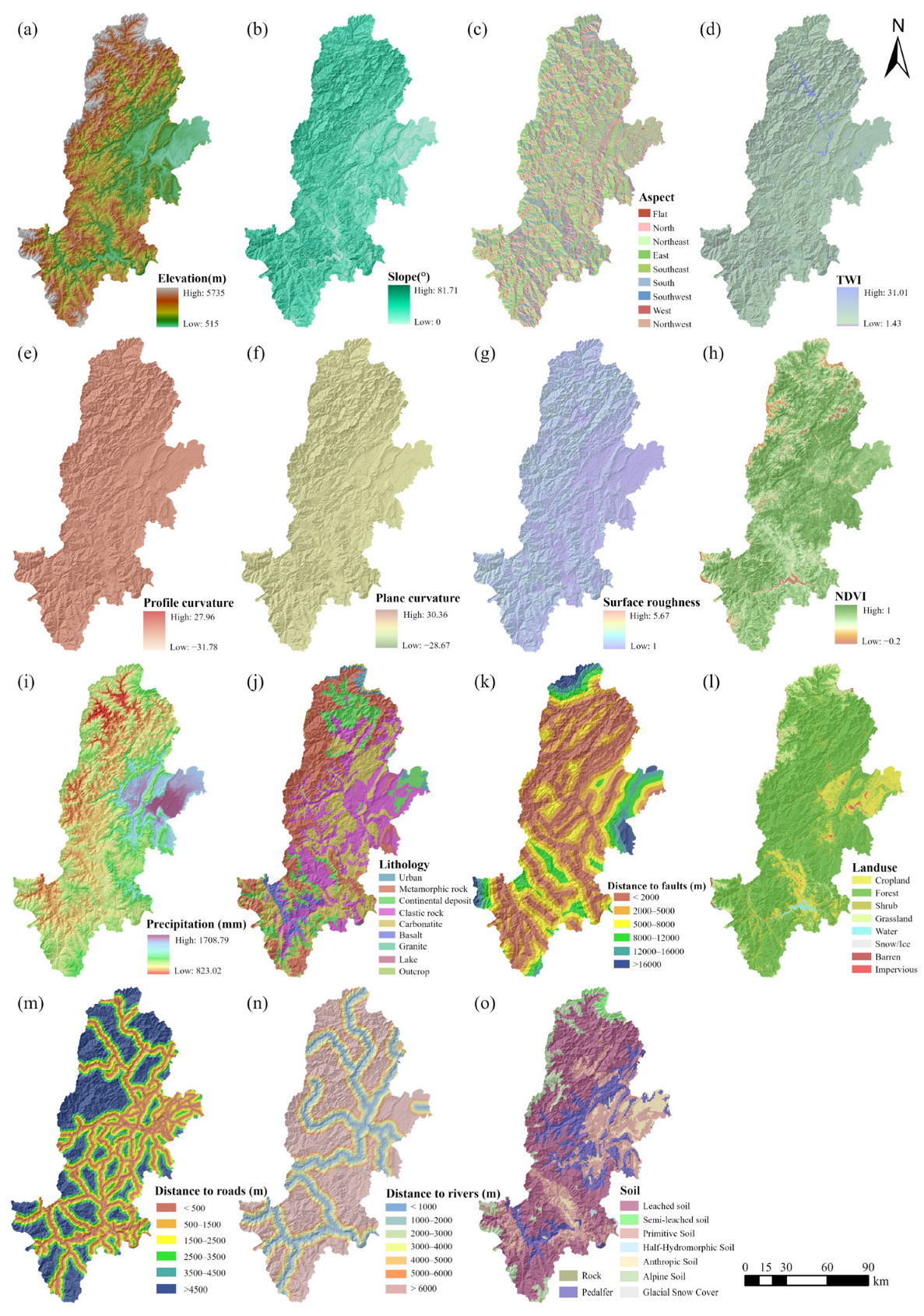
Landslide occurrence is strongly influenced by environmental conditions, which vary by region. Therefore, the selection of influencing factors must consider the specific characteristics of the study area. Based on regional features and previous studies, 15 evaluation factors were selected from four categories: topography, geological conditions, land cover, and hydrology. These factors include elevation, slope, aspect, profile curvature, plane curvature, TWI, surface roughness, lithology, distance to faults, NDVI, land use type, soil type, distance to roads, distance to rivers, and precipitation (Figure 2). The basic datasets were processed using ArcGIS (https://www.arcgis.com/) and MapGIS (https://mapgis-map-gis.hub.arcgis.com/) to extract the evaluation factors. All spatial layers were unified to a common coordinate system and resampled to a 30 m × 30 m resolution, resulting in 16,730,339 grid cells for subsequent analysis.
To assess the influence of conditioning factors on landslide development, the frequency ratio (FR) method was applied to quantify the correlation between landslide occurrences and each factor. Higher FR values indicate a stronger association with landslide susceptibility. Continuous variables were discretized using a combination of natural breaks and equal-interval methods. FR curves were then used to identify inflection points as classification thresholds, enabling a more robust stratification of continuous data [35]. Classification results are summarized in Table 2.
(1)
Topographic factors: These include elevation, slope, aspect, surface roughness, plane curvature, profile curvature, and the TWI. Aspect affects the amount of solar radiation received by slopes, thereby influencing moisture and temperature conditions, vegetation growth, and ultimately the spatial distribution of landslides [36]. Slope directly affects runoff, stability, and gravitational forces. Curvature metrics reflect terrain complexity and material transport [37]. Landslides are mainly concentrated in areas with elevation < 1300 m, slope < 28°, aspect < 250°, plan curvature [−0.8, 0.5), profile curvature [−0.4, 0.5), and TWI > 22.6—all corresponding to higher FR values.
(2)
Geological factors: Lithology and distance to faults significantly affect landslide potential. Landslides in the study area are primarily distributed in regions dominated by clastic rocks and carbonate rocks. Clastic rocks are highly weathered with high porosity and permeability, making them structurally weak and prone to failure. Carbonate rocks such as limestone and dolomite are susceptible to dissolution, which compromises rock integrity and facilitates the formation of potential sliding surfaces and fracture zones.
(3)
Land cover factors: NDVI, land use, soil type, and distance to roads influence landslide occurrence. High susceptibility is observed in areas with NDVI < 0.7, within 2500 m of roads, and land use types such as cultivated land and impervious surfaces. Soils like Entisols and anthropogenic soils further contribute to instability.
(4)
Hydrological factors: Distance to rivers and precipitation levels also play a key role. Areas within 4000 m of rivers and with annual precipitation > 1300 mm show elevated FR values, suggesting that excessive rainfall and proximity to water bodies increase the risk of slope saturation, reduced shear strength, and ultimately landslide initiation.

3.3. Methods

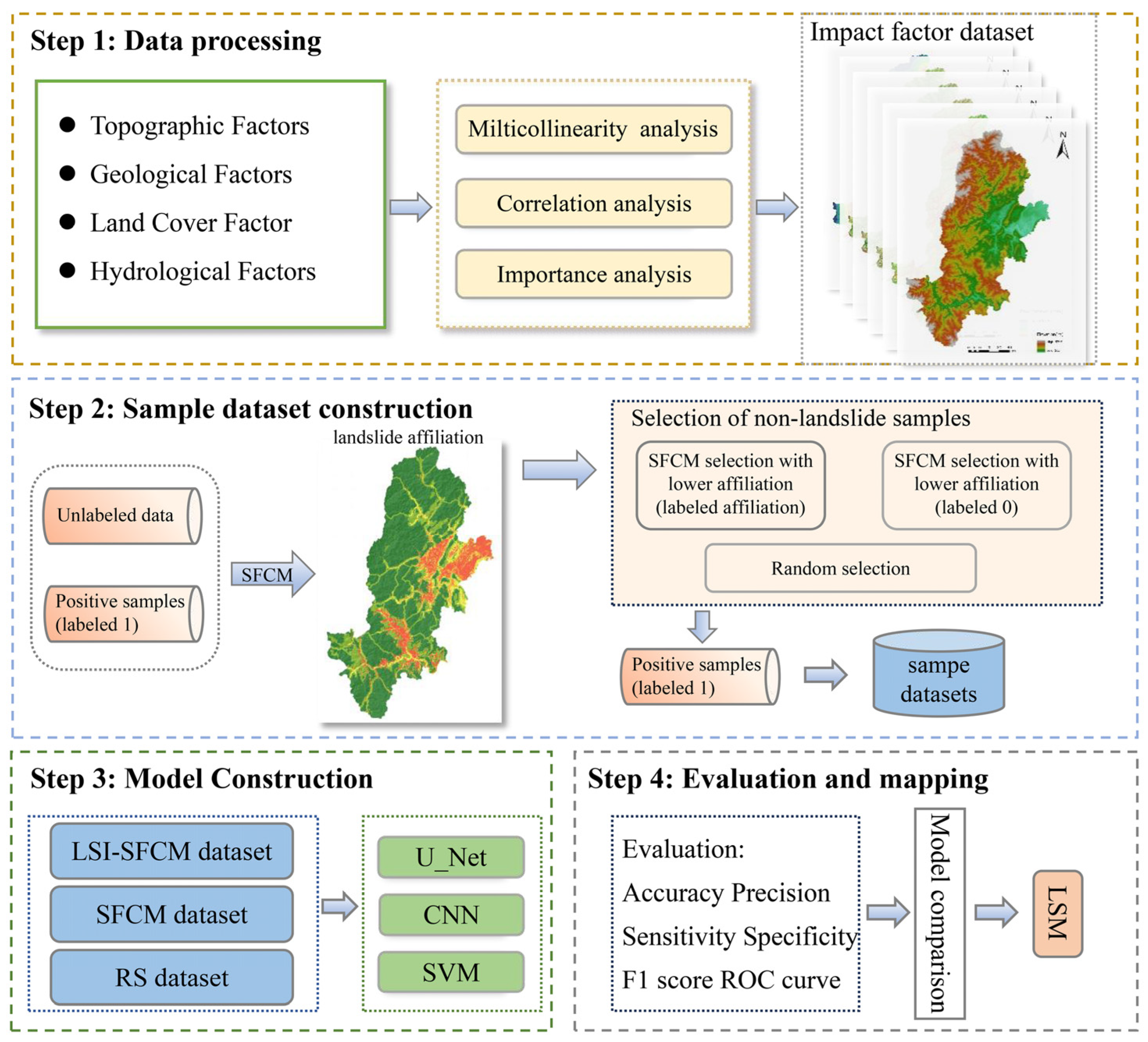
Historical landslide records provide crucial reference data for building reliable susceptibility models and identifying high-risk areas [38]. These records are typically used as positive samples (labeled as 1), offering relatively high accuracy. In contrast, the selection of negative samples remains uncertain. Traditional approaches typically assign a label of 0 to negative samples, effectively treating non-landslide areas as entirely risk-free. However, although these areas may not have yet met the triggering conditions for landslides, the possibility of future occurrences cannot be ruled out due to the presence of latent susceptibility factors [24]. To improve sample reliability and prediction accuracy, this study proposes a semi-supervised clustering-based strategy incorporating membership values for negative sample selection. The approach involves (1) reclassifying all conditioning factors and selecting key variables through multicollinearity, correlation, and importance analysis to construct a composite factor dataset. (2) Applying SFCM clustering with prior landslide knowledge to derive landslide membership values as initial LSI results. Negative samples were selected from low-membership areas: for the LSI-SFCM dataset, membership values were assigned as labels; for the SFCM and RS datasets, labels were set to 0 based on low-membership regions and random sampling outside landslide zones, respectively. (3) Training U-Net, CNN, and SVM models using the three datasets for landslide susceptibility prediction. (4) Evaluating model performance and generating susceptibility maps. The technical workflow is shown in Figure 3.

3.3.1. Semi-Supervised Fuzzy C-Means Clustering (SFCM)

Traditional clustering methods primarily rely on hard clustering, where each object is assigned to a single category, often leading to binary classification. However, when object features exhibit uncertainty or lack clear class boundaries, hard clustering can result in errors [39]. Fuzzy clustering, as a type of soft clustering, allows each object to have varying degrees of membership in different categories [40]. A higher membership value indicates a stronger association with that category, thereby effectively handling the ambiguity between classes.
The fuzzy C-means clustering (FCM) algorithm, proposed by Bezdek based on fuzzy set theory, has gained significant attention in research [41]. The SFCM algorithm was proposed by Pedrycz and Waletzky in 1997 as a semi-supervised extension of the FCM algorithm [42]. By incorporating a small amount of labeled data into the clustering process, SFCM enhances the clustering performance. The objective function of the SFCM algorithm is defined as follows:
J = i = 1 c j = 1 N u i j m d i j 2 + α i = 1 c j = 1 N ( u i j f i j b j ) m d i j 2
where m is the fuzziness index, an empirical parameter typically set to 2 [43,44]; α ( α ≥ 0) is a balancing parameter that adjusts the balance between unsupervised and supervised information; c i denotes the i-th cluster center; d i j = x j c i represents the Euclidean distance between the j-th sample x j and cluster center c i ; u i j is the membership degree of x j to cluster i ; f i j denotes the membership degree of labeled sample x j to cluster i ; b j is a Boolean variable indicating whether x j is a labeled sample (1 for labeled, 0 otherwise).
Under the conditions of satisfying the constraints, the Lagrange multiplier method is applied to the objective function J , yielding u i j and c i , as shown in the following equation:
u i j = 1 1 + α 1 + α 1 b j k = 1 c f k j k = 1 C d i j d k j 2 + α f i j b j
c i = j = 1 n ( u i j 2 x j ) + α j = 1 n u i j b j f i j 2 x j j = 1 n u i j 2 + α j = 1 n u i j b j f i j 2
The specific steps of the SFCM algorithm are as follows:
(1)
Incorporate labeled data into the dataset for initial partitioning and obtain the initial cluster centers;
(2)
Calculate the distance between all samples (both labeled and unlabeled) and the cluster centers. Then compute the initial membership matrix using Equation (2);
(3)
Compute the objective function value using Equation (1). If the value is below a predefined threshold or the change from the previous iteration is smaller than the threshold, stop the iteration and output the membership matrix and cluster centers;
(4)
Otherwise, update the cluster centers using Equation (3), return to step (2), and repeat the process until convergence.

3.3.2. Convolutional Neural Network (CNN)

CNN is a widely used deep learning model, extensively applied in image detection, speech recognition, and natural language processing [45]. The network structure consists of three parts: convolutional layers, pooling layers, and fully connected layers. The convolutional layer performs feature extraction on the input data by computing the input data with convolutional kernels, thereby generating feature maps. The convolution calculation formula is as follows:
C j = i N f w j × x i + b j , j = 1,2 , , k
where k represents the number of convolutional kernels; C j denotes the output of the j-th convolutional kernel; f is the nonlinear activation function; i indicates the spatial position of the convolution; x i is the input data to the convolutional layer; and w j and b j are the weights and biases, respectively.
The pooling layer, also known as downsampling, employs methods such as max pooling and average pooling. Its operational process is similar to that of convolution, extracting the most representative features to prevent overfitting, reduce parameters, and enhance the model’s generalization ability [46]. The fully connected layer flattens all extracted feature maps into a 1 × x vector, which partially loses spatial structure information. The final output is obtained by applying an activation function.
In the proposed LSI-SFCM sampling strategy, negative samples are assigned membership values derived from SFCM clustering, thereby transforming the original binary classification task into a regression problem for landslide probability. This “soft label” approach provides a more detailed characterization of the spatially continuous variation in landslide susceptibility. Compared to the traditional method of assigning all negative samples a label of 0, it helps to reduce the oversimplification of boundary samples. However, this approach also introduces a risk of semantic ambiguity in the labels, where the model may misclassify high-membership negative samples, potentially reducing its ability to distinguish true landslide instances. To mitigate this risk, early stopping and dropout regularization are applied during training to control model complexity and enhance generalization. In the validation phase, a threshold of 0.5 is set for binary determination based on the output probability values, enabling the calculation of evaluation metrics and ensuring both clarity and practical usability. The output layer consists of a single neuron with a sigmoid activation function, which outputs the landslide probability.

3.3.3. U-Net Model

The U-Net model is a variant of CNNs, originally developed for biomedical image segmentation [47]. It has since demonstrated strong adaptability in geospatial applications [48,49]. The model effectively captures spatial correlations among raster cells within local regions. Through skip connections between the encoder and decoder paths, it compensates for information loss during decoding. This allows the model to fully exploit and integrate abstract features from deep layers with contextual semantic information from shallow layers. U-Net offers strong feature learning capability and high prediction accuracy [50].
The U-Net model consists of an encoder–decoder structure, as shown in Figure 4. The left side is the encoder path, which includes several convolutional layers and max-pooling layers. The convolutional layers extract local features from the input image, while the pooling layers reduce redundant information, decrease computation, and improve processing speed. The operation of downsampling by convolution and pooling forms a pyramid of features from low to high dimensions [50]. The right side is the decoder path, which includes several convolutional layers and transposed convolution layers. The transposed convolution layers perform upsampling to generate feature maps corresponding to the original feature pyramid, with dimensions halved at each level [51]. Skip connections between the encoder and decoder paths fuse the decoder outputs with the feature maps from the symmetric positions in the encoder. This helps reduce gradient vanishing and recover lost information during decoding [52].
In this study, the LSI-SFCM-U-Net model is built based on the LSI-SFCM sample dataset. It outputs landslide susceptibility probabilities. In the final layer, a sigmoid activation function is used to generate prediction values in the range of 0 to 1. Values greater than 0.5 are considered positive samples, and values less than 0.5 are considered negative samples.

3.3.4. Support Vector Machine (SVM)

SVM is a supervised learning algorithm widely used for classification and regression tasks. Its core idea is to construct one or more hyperplanes to optimally separate data points. The goal is to maximize the margin between samples of different classes and find the optimal hyperplane [53]. In many complex classification and regression problems, data cannot be easily separated linearly. To address this, SVM introduces kernel functions (such as linear kernel and radial basis function kernel) to map data into a higher-dimensional feature space, where a linearly separable hyperplane can be constructed [54]. For regression tasks, SVM uses the ε-insensitive loss function to build the optimal regression plane. Only support vectors outside the ε-margin are considered, which helps control model complexity and improves robustness to noise [55].
In this study, the LSI-SFCM-SVM model was constructed based on the LSI-SFCM sample dataset. The SVR function from the sklearn library was used to handle the regression problem. Grid search was applied to find the optimal parameters (C = 1, γ = 0.1), and the model outputs reasonable landslide susceptibility probability values.

3.3.5. Evaluation Indicators

In this study, the accuracy, precision, recall, specificity, and F1-score were selected to measure model performance. Accuracy reflects the overall correctness of the model’s predictions across all samples. Precision indicates the proportion of true positive samples among all samples predicted as positive, while recall assesses the model’s ability to correctly identify positive samples. F1-Score combines both precision and recall, serving as a comprehensive performance metric [56]. The Receiver Operating Characteristic (ROC) curve is commonly used to assess overall performance, with the Area Under the Curve (AUC) indicating better performance with higher values [57]. The prediction rate curve is used to evaluate how well landslide samples fit the landslide susceptibility index (LSI) map by mapping landslide samples onto the susceptibility map [6]. First, the LSI values of the study area are sorted in descending order and divided into 20 equal intervals. Then, the number of landslide samples within each interval is calculated. Finally, a curve is plotted with the interval rank on the x-axis and the cumulative percentage of landslides on the y-axis [58]. The area under the prediction rate curve (AUC) is used as an evaluation metric, with higher values indicating better prediction accuracy. The evaluation metric is defined as follows:
A c c u r a c y = T P + T N F P + F N + T P + T N
P r e c i s i o n = T P T P + F P
R e c a l l = T P T P + F N
S p e c i f i c i t y = T N T N + F P
F 1 _ S o c r e = 2     P r e c i s i o n     R e c a l l P r e c i s i o n + R e c a l l
where T P denotes the number of positive samples correctly categorized, T N denotes the number of negative samples correctly categorized, F P denotes the number of negative samples incorrectly categorized, and F N denotes the number of positive samples incorrectly categorized.

4. Landslide Susceptibility Assessment

4.1. Influencing Factors Screening

Multicollinearity may exist among the initially selected landslide influencing factors. Including all factors in the model can make it difficult to accurately determine their relative contributions, leading to imbalanced weight assignment, which may interfere with model training and result in unstable predictions [59]. To ensure the independence of selected factors, the variance inflation factor (VIF) and tolerance (TOL) were first used to assess multicollinearity. A VIF greater than 10 or a TOL less than 0.1 indicates significant multicollinearity among factors [60]. Pearson correlation coefficients were then used for further verification. A correlation coefficient greater than 0.5 suggests a strong relationship between factors, which should be removed or adjusted [61].
Table 3 and Figure 5 show the VIF values and Pearson correlation coefficients of the initial factors. All VIF values are below 10, indicating no strong multicollinearity. However, the correlation results show that elevation has strong correlations (absolute values > 0.5) with lithology, soil type, and distance to roads. The correlation coefficient between slope and surface roughness is 0.81, and the absolute correlation between plane curvature and profile curvature is also greater than 0.5. As elevation is strongly correlated with multiple factors, it was excluded. The other two highly correlated pairs were evaluated using importance analysis to decide which to retain.
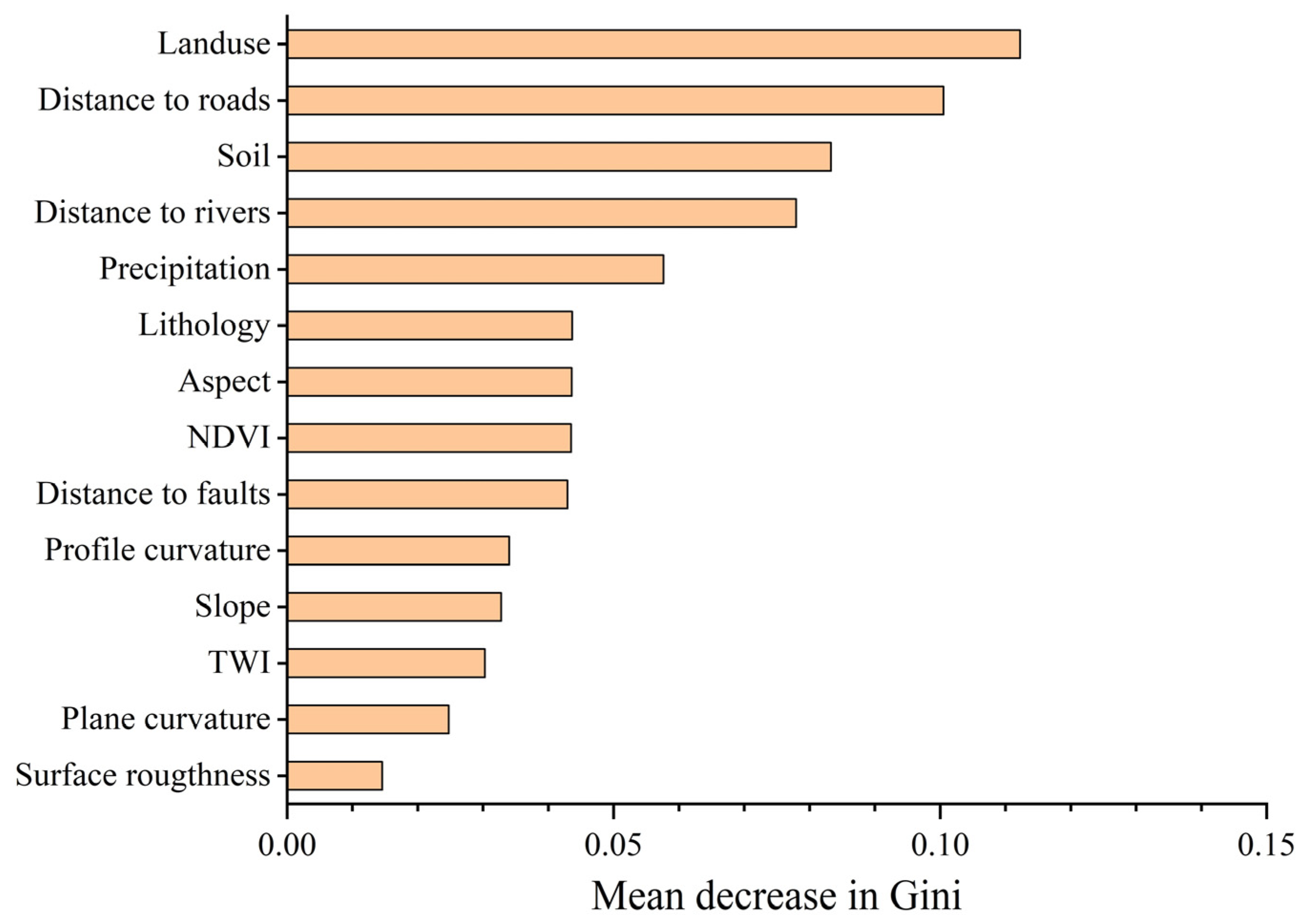
Including factors with limited impact on landslides may introduce redundant information and reduce the efficiency of model training and prediction. To improve model accuracy, this study used the ‘RandomForestRegressor’ module from scikit-learn to analyze the importance of landslide conditioning factors. As shown in Figure 6, land use type had the highest importance score (0.11), followed by distance to roads. Surface roughness and plane curvature had the lowest importance, both below 0.03. Additionally, the previous correlation analysis revealed strong correlations between slope and surface roughness, plane curvature, and profile curvature. Therefore, plane curvature and surface roughness—both with low importance—were excluded.
In summary, elevation, surface roughness, and plane curvature were excluded based on multicollinearity, Pearson correlation, and importance analysis. The final 12 selected conditioning factors used for landslide susceptibility analysis are: slope, aspect, precipitation, profile curvature, TWI, lithology, distance to faults, NDVI, land use, soil type, distance to roads, and distance to rivers.

4.2. Selection of Non-Landslide Samples Based on SFCM

In this study, the SFCM algorithm was employed during the non-landslide sample selection phase, which can effectively deal with the ambiguity problem. Similar fuzzy or semi-supervised approaches have been widely applied in geospatial modeling to handle data uncertainty and improve classification accuracy. For instance, Huang et al. proposed a semi-supervised imbalanced sampling strategy that selects reliable non-landslide samples from low-susceptibility areas and uses soft labels to enhance model accuracy [24]. Parsian et al. applied a fuzzy logic-based framework combined with AHP weighting to integrate multiple remote sensing and GIS factors, achieving over 95% prediction accuracy [62]. These studies demonstrate that fuzzy labeling can enhance model interpretability and robustness by capturing susceptibility rather than rigid binary labels. Our SFCM-based strategy aligns with these approaches by using fuzzy membership to construct more representative training samples, thereby supporting more reliable susceptibility predictions in this section.
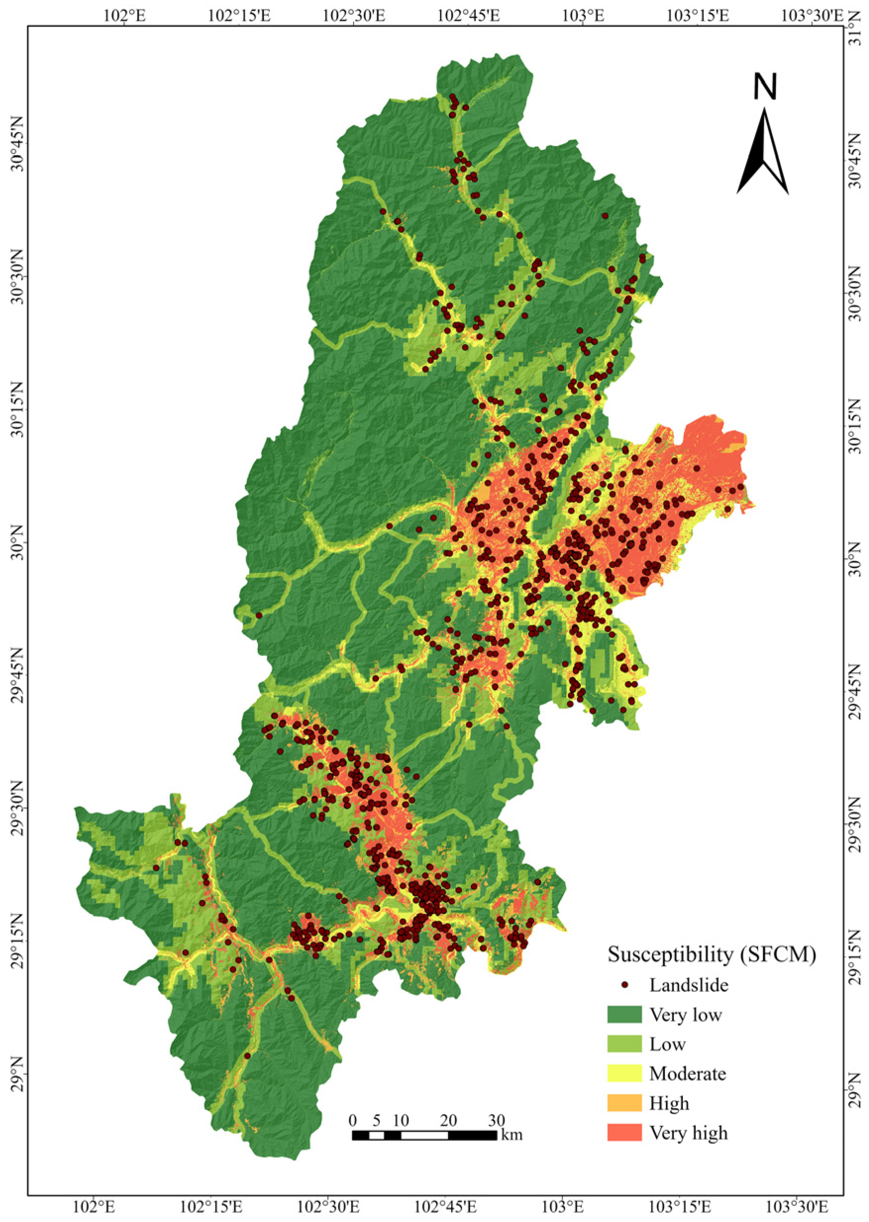
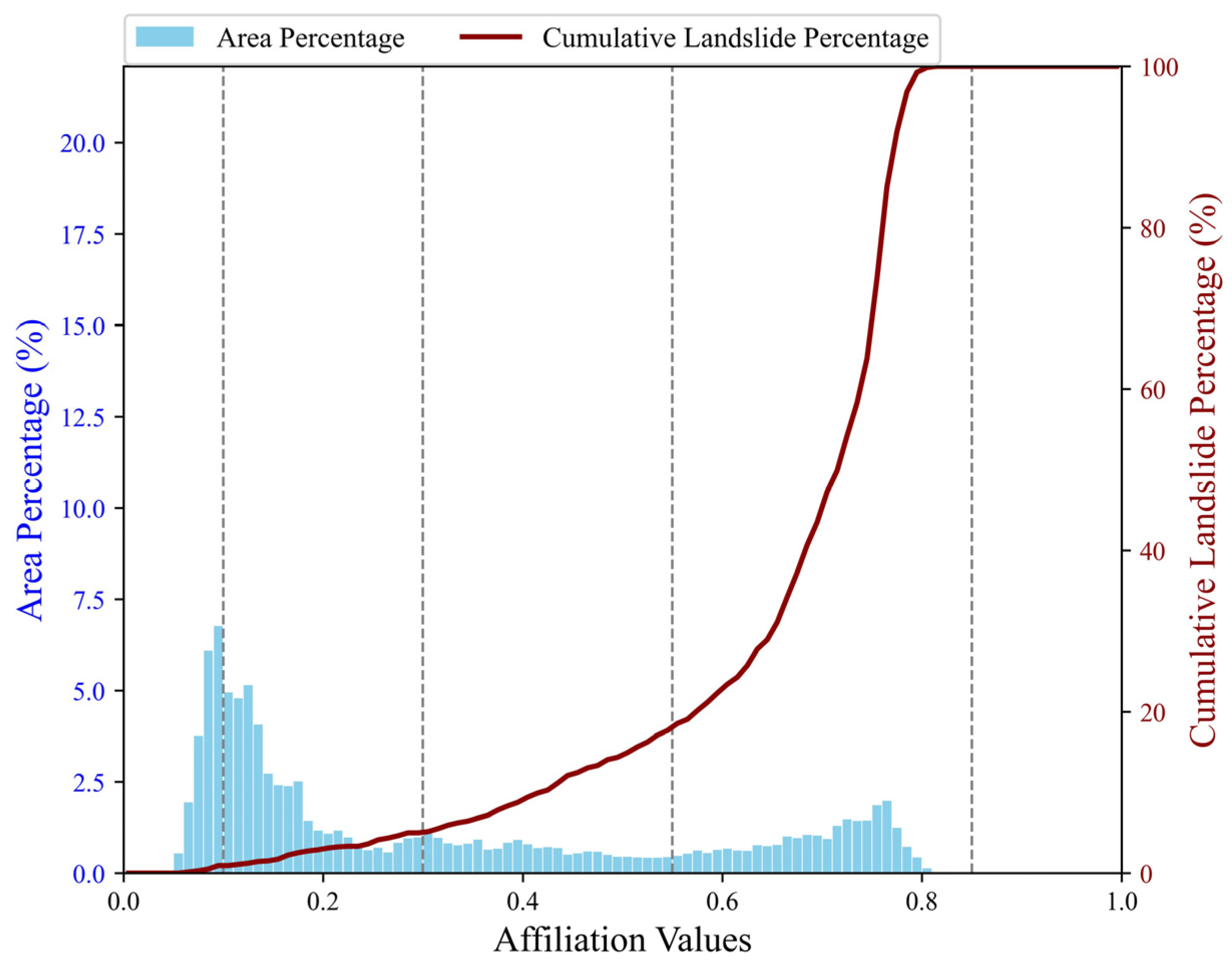
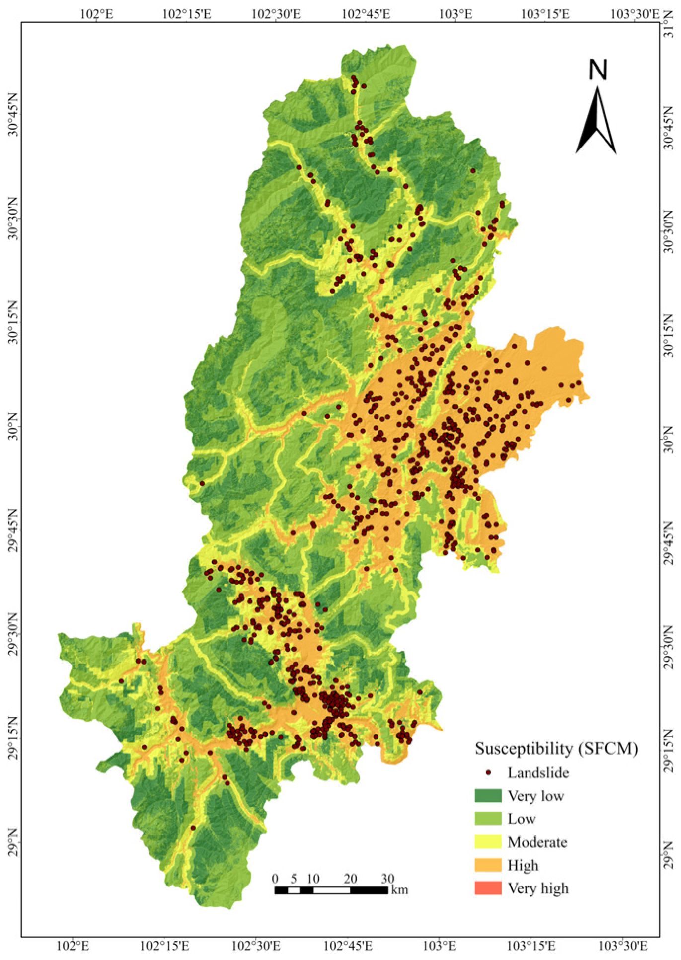
Twelve selected landslide conditioning factors were used as input data, along with the frequency ratio and labeled positive samples. The number of clusters C was set to 2 to distinguish between landslide and non-landslide classes, which helps improve the clarity and interpretability of the clustering results. The clustering process was guided by known sample information, and the cluster centers and membership matrix were iteratively optimized until the objective function reached the minimum threshold. The membership degree of the landslide class was used as the initial LSI. The LSI distribution and the cumulative percentage curve of landslides are shown in Figure 7. Based on the membership degree of each unit, the study area was classified into five susceptibility levels: very low (0–0.1), low (0.1–0.3), moderate (0.3–0.55), high (0.55–0.85), and very high (0.85–1), as shown in Figure 8.
According to Figure 7, the cumulative percentage curve of landslides rises slowly at low membership values but increases sharply in the range of 0.85–1. In this range, landslides account for 52% of the total, while the corresponding area proportion is relatively small. In contrast, areas with low membership values cover a large proportion of the total area. This is consistent with the general pattern of landslide occurrence, where landslides remain low-probability events across the entire study area [63]. As shown in Figure 8, the spatial distribution of landslide susceptibility indicates that high-susceptibility areas are mainly concentrated in the eastern and southeastern parts. Very high and high susceptibility zones are distributed in strips along roads and rivers. These areas are characterized by low elevation, high rainfall, dense road and clastic rock distribution, low vegetation cover, and intensive human activities, resulting in high landslide risk. This pattern is consistent with the historical distribution of landslides, indicating that the SFCM algorithm effectively identifies landslide-prone features and produces reasonable susceptibility results.
To exclude high-susceptibility landslide areas while ensuring sample diversity and avoiding spatial clustering effects, non-landslide samples equal in number to the positive samples were selected from areas with membership degrees below 0.55 to form multiple negative sample sets. Specifically, (1) the membership values of the selected negative samples were used as their labels and combined with positive samples to construct the LSI-SFCM dataset; (2) the selected negative samples were assigned a uniform label of 0 and combined with positive samples to form the SFCM dataset; (3) an equal number of negative samples were randomly selected, labeled as 0, and combined with positive samples to create the RS dataset. These three sample construction strategies were used for subsequent landslide susceptibility modeling and comparative analysis.

4.3. Model Accuracy Analysis

All sample datasets were divided into training and testing sets at a ratio of 7:3 for model training and testing. The optimal hyperparameters for each model were obtained using grid search. Table 4 shows the accuracy results of each model under the three sampling strategies.
The results show that the LSI-SFCM strategy outperforms both the SFCM and RS strategies across evaluation metrics, demonstrating superior overall performance. In particular, the U-Net model achieved the highest accuracy (0.902), specificity (0.921), and F1-score (0.886), indicating strong classification capability. The SFCM strategy performed best in terms of precision, reaching a maximum value of 0.901 with the SVM model. However, its recall and specificity were slightly lower than those of LSI-SFCM. This is mainly due to the strict boundary classification mechanism of the SVM model, which makes positive predictions more conservative, effectively reducing false positives but at the cost of lower recall. In comparison, the RS strategy showed generally lower performance across all models. Notably, the SVM model under RS yielded the lowest specificity (0.727) and precision (0.747), indicating that traditional random negative sampling has certain limitations in ensuring model prediction performance.
Figure 9 shows the ROC curves of different models under various sampling strategies. All models achieved AUC values above 85%, indicating good prediction performance. Under the LSI-SFCM sampling strategy, each model achieved higher AUC values than under the other two strategies, suggesting better predictive capability. In addition, under all three sampling strategies, deep learning models (U-Net and CNN) performed better than the SVM model in terms of AUC. Among them, the LSI-SFCM-CNN model (AUC = 95.52%) ranked second only to the LSI-SFCM-U-Net model (AUC = 95.85%), followed by the LSI-SFCM-SVM model (AUC = 94.95%). All three models showed the lowest performance under the RS sampling strategy. These results indicate that the LSI-SFCM sampling strategy improves model prediction accuracy, and the U-Net model performs better than the CNN and SVM models.
Figure 10 shows the prediction rate curves of different models under various sampling strategies. Overall, the LSI-SFCM strategy achieved the best performance across all models. The prediction rate of the CNN model reached 0.859, followed by U-Net (0.837) and SVM (0.817), all higher than the other two strategies. Under this strategy, the prediction rate curve rises steeply at the beginning, indicating that the models can effectively identify high-susceptibility landslide areas and better capture spatial distribution patterns. In the SFCM strategy, non-landslide samples were labeled as 0. Although the AUCs of CNN, U-Net, and SVM reached 94.28%, 94.80%, and 92.76%, respectively, their prediction rates were lower than those of the LSI-SFCM strategy (0.809, 0.808, and 0.766). This difference suggests that assigning a fixed value of 0 to non-landslide areas may limit the model’s ability to learn spatial variability, potentially leading to overfitting and inaccurate risk estimation. In comparison, the RS strategy showed the worst performance in all models, with the lowest AUC and prediction rate values. This indicates that random sampling failed to reflect the spatial patterns of landslide occurrence, weakening the model’s ability to identify high-susceptibility areas. In addition, labeling all non-landslide samples as 0 further reduced the model’s sensitivity to potential risks in these areas.
It is worth noting that the prediction rate curves of the SVM model were less smooth compared to CNN and U-Net. The curve rose slowly in the early stage and accelerated slightly later. This may be due to the SVM’s reliance on support vectors, making it more sensitive to data distribution and less effective in capturing complex spatial heterogeneity and nonlinear features. In summary, the LSI-SFCM sampling strategy improved the model’s recognition of spatial patterns and prediction accuracy. Among the models, CNN performed the best and is more suitable for landslide susceptibility prediction in complex geological environments.

4.4. Results of Landslide Susceptibility Mapping (LSM)

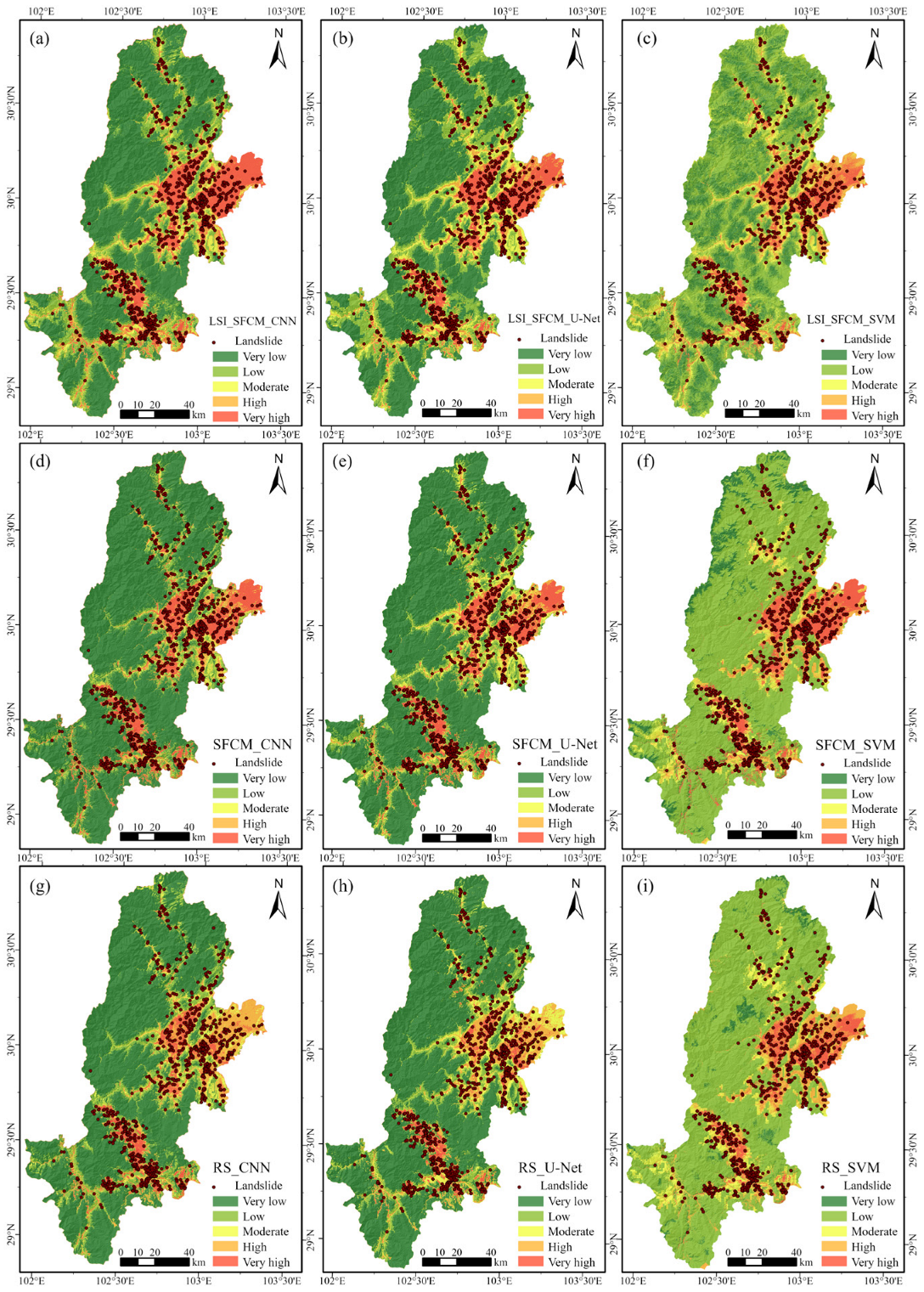
The twelve landslide conditioning factors were input into the trained models for prediction. Based on the statistical distribution of the predicted probability values and previous studies [64,65], the study area was classified into five susceptibility levels: very low (0–0.1), low (0.1–0.3), moderate (0.3–0.55), high (0.55–0.85), and very high (0.85–1). The results are shown in Figure 11.
Overall, the prediction results of all models exhibited similar spatial distribution patterns. High-susceptibility zones were mainly concentrated in the eastern and southeastern areas, where roads are densely interlaced, river systems are well-developed, rainfall is abundant, and human activities are intensive—making landslides more likely. Compared with machine learning models, deep learning models identified larger areas as very low susceptibility zones, which better excludes potential landslide hazards. To further evaluate the reliability of the susceptibility mapping results, the number of landslides and the area percentage within each susceptibility zone were calculated, as shown in Table 5 and Table 6.
As shown in Table 5 and Table 6, under the LSI-SFCM sampling strategy, all models successfully covered more than 74% of landslide points in the very high susceptibility zone, significantly outperforming the SFCM and RS strategies. This indicates a stronger ability to identify landslides. Meanwhile, the area proportion of the very low susceptibility zone remains high, with a very low number of landslides in that zone. This effectively avoids misclassifying high-risk areas as low-risk and reduces false alarms. In contrast, although the SFCM and RS strategies show slightly higher area proportions in the very low susceptibility zone, the number of landslides in these areas is also higher. This suggests that the models may underestimate the risk in these zones and show a more conservative prediction pattern. Especially under the RS strategy, the very high susceptibility zone has a clearly lower area proportion, resulting in insufficient coverage of landslide points and a higher risk of missed alarms.
Overall, although the LSI-SFCM strategy results in a larger area of very high susceptibility, it captures more actual landslide points and significantly reduces the risk of missing high-risk zones. In practical applications, moderate overestimation of high-risk areas is acceptable compared to the severe consequences of missed predictions. Therefore, the LSI-SFCM-based results offer better risk control value and are more meaningful for landslide disaster prevention and mitigation.

5. Discussion

5.1. Discussion on the Semi-Supervised Sampling Strategy

Traditional random sampling methods are easy to implement but have notable limitations in landslide susceptibility modeling. They often misclassify high-risk areas as negative samples, reducing the representativeness of the dataset and affecting the model’s discrimination ability and prediction accuracy [66]. Low-slope and buffer-based sampling can partly avoid high-risk areas. However, the former often leads to uneven spatial distribution and limited feature diversity, while the latter depends on user-defined buffer distances, which lack objective justification and introduce subjectivity [67]. In recent years, unsupervised clustering has attracted increasing attention due to its independence from large-scale manual labeling. In LSA, unsupervised clustering can automatically divide potential categories based on the similarity of sample attributes, providing a possible way to identify landslide and non-landslide areas [68]. However, most existing methods, such as K-means, are hard clustering algorithms. They only output fixed category labels and cannot express the uncertainty of sample membership. This limitation is particularly problematic in transition zones near landslide boundaries, where geological conditions are inherently ambiguous. Moreover, clustering without prior knowledge often deviates from the actual landslide distribution, reducing the representativeness of selected samples and the generalization of the model.
This study uses a semi-supervised clustering method that incorporates membership values to select non-landslide samples. By introducing labeled landslide samples to guide the clustering process, the model generates membership information indicating the likelihood of belonging to the landslide class. This approach improves the representativeness and rationality of non-landslide samples.
Figure 12 and Figure 13 show the cumulative curve and membership distribution of landslides generated by the unsupervised FCM algorithm. The results indicate that FCM membership values are mainly concentrated in low, moderate, and high susceptibility areas, while the proportion of areas with very high or very low susceptibility is relatively small. This leads to weak model learning in high-confidence zones. In low-membership regions, although the cumulative curve is flatter, the small area coverage may cause the model to underestimate the risk in low-susceptibility areas. These findings reflect the limitations of FCM in capturing feature diversity among non-landslide samples. In contrast, the SFCM approach provides a more continuous membership distribution and preserves greater variability in areas of very low susceptibility, demonstrating stronger capability in expressing spatial heterogeneity.
Based on this, the LSI-SFCM dataset is constructed using membership values instead of traditional binary labels for negative samples. This enhances the representation of fuzzy class boundaries in the training data and reduces classification errors caused by hard labeling. Compared with traditional random sampling (RS), LSI-SFCM more accurately captures the spatial patterns of landslide occurrence. Compared with SFCM without membership information, this strategy adds uncertainty information to negative samples, improving the model’s ability to distinguish non-landslide areas, reducing false alarms, and increasing adaptability under complex terrain conditions.

5.2. Discussion of the Landslide Susceptibility Mapping

The LSI-SFCM sampling strategy exhibits a more conservative pattern in landslide susceptibility mapping, characterized by a slight decrease in the proportion of areas classified as “very low” susceptibility and an increase in the “high” and “very high” categories. This shift does not represent a systematic bias, but rather reflects the model’s enhanced capacity to identify latent risk zones that might be underestimated by conventional methods. In contrast to conventional random sampling, which is typically based solely on the geospatial sampling schemes and may mistakenly include potentially hazardous areas as negative samples, thereby weakening the model’s ability to identify true landslide-prone regions. The LSI-SFCM approach integrates both spatial and attribute information. By incorporating landslide probability labels, it avoids extreme labeling, enriches the information of negative samples, and improves their reliability. Although it slightly reduces the area classified as “very low” susceptibility, it ensures better coverage of high-risk zones and minimizes the risk of false negatives. This trade-off is acceptable in practical hazard mapping, as it prioritizes the identification of vulnerable areas and supports public safety. Evaluation results across multiple models further confirm the validity of this shift. The LSI-SFCM strategy consistently yields higher AUC and prediction rates without compromising performance in low-susceptibility areas.

5.3. Limitations and Future Work

Although the proposed semi-supervised clustering sampling strategy based on membership information significantly improved model performance and generated a more reasonable spatial distribution of landslide susceptibility, some limitations remain and should be addressed in future work:
(1)
The selected landslide conditioning factors in this study cover topography, geological environment, land cover, hydrology, and human activities, forming a relatively comprehensive system. However, the variables related to human activities are limited and do not fully reflect external disturbances such as engineering construction. This restricts the model’s sensitivity and generalization to human-induced landslides. Future studies should incorporate more indicators of human activity intensity, such as road density, engineering activity frequency, and settlement density, to enhance model adaptability under complex human disturbances.
(2)
Deep learning models (e.g., U-Net and CNN) showed high accuracy and strong ability in capturing spatial patterns, especially excelling in modeling complex nonlinear features. However, they require substantial computational resources and prediction time, which limits their large-scale application. Moreover, their “black-box” nature reduces interpretability and trust in real-world disaster management. Future work should focus on developing lightweight network architectures to balance predictive performance with computational efficiency. In addition, attention mechanisms and explainable AI techniques—such as SHAP—should be employed to investigate internal feature contributions, thereby enhancing model interpretability, transparency, and trustworthiness in landslide risk management.
(3)
In this study, the number of non-landslide samples was set equal to that of landslide samples to control for class imbalance effects and isolate the influence of the sampling strategy. While the quantity of non-landslide samples is known to affect susceptibility mapping outcomes, particularly in imbalanced data settings, this factor was intentionally held constant in order to focus the analysis on sampling strategy performance. Future studies may extend this work by exploring how varying non-landslide sample ratios impact model accuracy, stability, and generalization.
(4)
Although the LSI-SFCM sampling strategy effectively enriches the feature representation of non-landslide samples and improves model performance, its reproducibility and adaptability to other geographic regions or hazard domains require further investigation. Landslide susceptibility modeling involves multiple stages—including sample construction, factor selection, and model design—each of which may introduce uncertainty and error. In particular, under conditions of sparse or noisy ground truth data (e.g., incomplete landslide inventories or uncertain labels), model robustness and generalizability may be compromised. To address this, future studies may explore integrating the proposed method with transfer learning, semi-supervised or weakly supervised frameworks, leveraging auxiliary data sources and applying data augmentation techniques to enhance model resilience and extend its applicability to broader, data-limited environments.

6. Conclusions

To address the issues of poor representativeness of traditional negative samples and unreasonable label assignment, this study proposes a semi-supervised clustering sampling strategy incorporating landslide membership information (LSI-SFCM). This strategy was applied to U-Net, CNN, and SVM models. The prediction performance and spatial distribution rationality of the models were systematically evaluated under three different sampling strategies. The results show that: (1) Sampling strategy has a significant impact on model performance. Models based on LSI-SFCM achieved the highest AUC values on the test set—95.85%, 95.52%, and 94.95%—and outperformed other strategies in prediction accuracy and spatial distribution. The strategy effectively enhances the representativeness and diversity of negative samples. (2) Compared with the unsupervised FCM algorithm, the SFCM method, incorporating prior landslide information, better distinguishes between landslide and non-landslide samples. The resulting susceptibility distribution aligns more closely with actual landslide patterns. (3) All three models performed well in LSA. Deep learning models (U-Net and CNN) showed better stability and evaluation capability. Nevertheless, their high computational cost and limited interpretability remain key challenges. Future work should explore lightweight architectures and explainable AI techniques to improve model efficiency and transparency. Consequently, the proposed LSI-SFCM strategy provides a valuable reference for disaster risk reduction. It holds promise for supporting early warning systems and land-use planning, thereby contributing to informed decision-making in hazard-prone regions.

Author Contributions

H.X. and Z.Q. designed research; H.X. and Y.L. performed research; H.X. and Y.T. analyzed data; H.X. wrote the paper; Y.T., R.Z. and H.L. revised it critically for important intellectual content. All authors have read and agreed to the published version of the manuscript.

Funding

This work was supported in part by the National Natural Science Foundation of China under grant 42301102 and the Gansu Youth Science and Technology Fund Program under grant no. 24JRRA100.

Data Availability Statement

The data presented in this study are available on request from the corresponding author.

Acknowledgments

Thanks Songwei Gu for providing valuable revisions in the study to improve the article.

Conflicts of Interest

All authors certify that they have no affiliations with or involvement in any organization or entity with any financial interest or non-financial interest in the subject matter or materials discussed in this manuscript.

References

  1. Huang, F.; Chen, J.; Liu, W.; Huang, J.; Hong, H.; Chen, W. Regional rainfall-induced landslide hazard warning based on landslide susceptibility mapping and a critical rainfall threshold. Geomorphology 2022, 408, 108236. [Google Scholar] [CrossRef]
  2. Li, Y.; Wang, X.; Mao, H. Influence of human activity on landslide susceptibility development in the Three Gorges area. Nat. Hazards 2020, 104, 2115–2151. [Google Scholar] [CrossRef]
  3. Gizzi, F.T.; Bentivenga, M.; Lasaponara, R.; Danese, M.; Potenza, M.R.; Sileo, M.; Masini, N. Natural Hazards, Human Factors, and “Ghost Towns”: A Multi-Level Approach. Geoheritage 2019, 11, 1533–1565. [Google Scholar] [CrossRef]
  4. Gamperl, M.; Singer, J.; Garcia-Londoño, C.; Seiler, L.; Castañeda, J.; Cerón-Hernandez, D.; Thuro, K. Recommendations for Landslide Early Warning Systems in Informal Settlements Based on a Case Study in Medellín, Colombia. Land 2023, 12, 1451. [Google Scholar] [CrossRef]
  5. Fell, R.; Corominas, J.; Bonnard, C.; Cascini, L.; Leroi, E.; Savage, W.Z. Guidelines for landslide susceptibility, hazard and risk zoning for land use planning. Eng. Geol. 2008, 102, 85–98. [Google Scholar] [CrossRef]
  6. Chung, C.-J.; Fabbri, A.G. Predicting landslides for risk analysis—Spatial models tested by a cross-validation technique. Geomorphology 2008, 94, 438–452. [Google Scholar] [CrossRef]
  7. Xu, S.; Song, Y.; Hao, X. A Comparative Study of Shallow Machine Learning Models and Deep Learning Models for Landslide Susceptibility Assessment Based on Imbalanced Data. Forests 2022, 13, 1908. [Google Scholar] [CrossRef]
  8. Hong, H.; Pradhan, B.; Sameen, M.I.; Chen, W.; Xu, C. Spatial prediction of rotational landslide using geographically weighted regression, logistic regression, and support vector machine models in Xing Guo area (China). Geomat. Nat. Hazards Risk 2017, 8, 1997–2022. [Google Scholar] [CrossRef]
  9. Lu, M.; Tay, L.T.; Mohamad-Saleh, J. Landslide susceptibility analysis using random forest model with SMOTE-ENN resampling algorithm. Geomat. Nat. Hazards Risk 2024, 15, 2314565. [Google Scholar] [CrossRef]
  10. Huang, F.; Cao, Z.; Jiang, S.-H.; Zhou, C.; Huang, J.; Guo, Z. Landslide susceptibility prediction based on a semi-supervised multiple-layer perceptron model. Landslides 2020, 17, 2919–2930. [Google Scholar] [CrossRef]
  11. Moayedi, H.; Mehrabi, M.; Mosallanezhad, M.; Rashid, A.S.A.; Pradhan, B. Modification of landslide susceptibility mapping using optimized PSO-ANN technique. Eng. Comput. 2019, 35, 967–984. [Google Scholar] [CrossRef]
  12. Xiao, X.; Zou, Y.; Huang, J.; Luo, X.; Yang, L.; Li, M.; Yang, P.; Ji, X.; Li, Y. An interpretable model for landslide susceptibility assessment based on Optuna hyperparameter optimization and Random Forest. Geomat. Nat. Hazards Risk 2024, 15, 2347421. [Google Scholar] [CrossRef]
  13. Khuc, T.D.; Truong, X.Q.; Nguyen, A.B.; Phi, T.T. Application of potential machine learning models in landslide susceptibility assessment: A case study of Van Yen district, Yen Bai province, Vietnam. Quat. Sci. Adv. 2024, 14, 100181. [Google Scholar] [CrossRef]
  14. Andrieu, C.; De Freitas, N.; Doucet, A.; Jordan, M.I. An introduction to MCMC for machine learning. Mach. Learn. 2003, 50, 5–43. [Google Scholar] [CrossRef]
  15. Sameen, M.I.; Pradhan, B.; Lee, S. Application of convolutional neural networks featuring Bayesian optimization for landslide susceptibility assessment. Catena 2020, 186, 104249. [Google Scholar] [CrossRef]
  16. Qin, Z.; Zhou, X.; Li, M.; Tong, Y.; Luo, H. Landslide susceptibility mapping based on resampling method and FR-CNN: A case study of Changdu. Land 2023, 12, 1213. [Google Scholar] [CrossRef]
  17. Tong, Y.X.; Luo, H.X.; Qin, Z.L.; Xia, H.; Zhou, X.Y. Enhanced Landslide Susceptibility Assessment in Western Sichuan Utilizing DCGAN-Generated Samples. Land 2025, 14, 34. [Google Scholar] [CrossRef]
  18. Chen, C.; Fan, L. Selection of contributing factors for predicting landslide susceptibility using machine learning and deep learning models. Stoch. Environ. Res. Risk Assess. 2023. [Google Scholar] [CrossRef]
  19. Chang, Z.L.; Huang, J.S.; Huang, F.M.; Bhuyan, K.; Meena, S.R.; Catani, F. Uncertainty analysis of non-landslide sample selection in landslide susceptibility prediction using slope unit-based machine learning models. Gondwana Res. 2023, 117, 307–320. [Google Scholar] [CrossRef]
  20. Liu, J.; Liang, E.; Xu, S.; Liu, M.; Wang, Y.; Zhang, F.; Luo, A. Multi-kernel support vector machine considering sample optimization selection for analysis and evaluation of landslide disaster susceptibility. Acta Geod. Et Cartogr. Sin. 2022, 51, 2034. [Google Scholar] [CrossRef]
  21. Imtiaz, I.; Umar, M.; Latif, M.; Ahmed, R.; Azam, M. Landslide susceptibility mapping: Improvements in variable weights estimation through machine learning algorithms—A case study of upper Indus River Basin, Pakistan. Environ. Earth Sci. 2022, 81, 112. [Google Scholar] [CrossRef]
  22. Lucchese, L.V.; de Oliveira, G.G.; Pedrollo, O.C. Investigation of the influence of nonoccurrence sampling on landslide susceptibility assessment using Artificial Neural Networks. Catena 2021, 198, 105067. [Google Scholar] [CrossRef]
  23. Kavzoglu, T.; Sahin, E.K.; Colkesen, I. Landslide susceptibility mapping using GIS-based multi-criteria decision analysis, support vector machines, and logistic regression. Landslides 2014, 11, 425–439. [Google Scholar] [CrossRef]
  24. Huang, F.; Xiong, H.; Jiang, S.-H.; Yao, C.; Fan, X.; Catani, F.; Chang, Z.; Zhou, X.; Huang, J.; Liu, K. Modelling landslide susceptibility prediction: A review and construction of semi-supervised imbalanced theory. Earth-Sci. Rev. 2024, 250, 104700. [Google Scholar] [CrossRef]
  25. Dou, H.; He, J.; Huang, S.; Jian, W.; Guo, C. Influences of non-landslide sample selection strategies on landslide susceptibility mapping by machine learning. Geomat. Nat. Hazards Risk 2023, 14, 2285719. [Google Scholar] [CrossRef]
  26. Wang, C.H.; Lin, Q.G.; Wang, L.B.; Jiang, T.; Su, B.D.; Wang, Y.J.; Mondal, S.K.; Huang, J.L.; Wang, Y. The influences of the spatial extent selection for non-landslide samples on statistical-based landslide susceptibility modelling: A case study of Anhui Province in China. Nat. Hazards 2022, 112, 1967–1988. [Google Scholar] [CrossRef]
  27. Liu, M.M.; Liu, J.P.; Xu, S.H.; Zhou, T.; Ma, Y.; Zhang, F.H.; Konecny, M. Landslide susceptibility mapping with the fusion of multi-feature SVM model based FCM sampling strategy: A case study from Shaanxi Province. Int. J. Image Data Fusion 2021, 12, 349–366. [Google Scholar] [CrossRef]
  28. Chang, L.; Xing, G.; Yin, H.; Fan, L.; Zhang, R.; Zhao, N.; Huang, F.; Ma, J. Landslide susceptibility evaluation and interpretability analysis of typical loess areas based on deep learning. Nat. Hazards Res. 2023, 3, 155–169. [Google Scholar] [CrossRef]
  29. Liang, Z.; Wang, C.M.; Duan, Z.J.; Liu, H.L.; Liu, X.Y.; Khan, K.U.J. A Hybrid Model Consisting of Supervised and Unsupervised Learning for Landslide Susceptibility Mapping. Remote Sens. 2021, 13, 1464. [Google Scholar] [CrossRef]
  30. Cai, J.; Hao, J.; Yang, H.; Zhao, X.; Yang, Y. A review on semi-supervised clustering. Inf. Sci. 2023, 632, 164–200. [Google Scholar] [CrossRef]
  31. Zhang, B.; Huang, L.; Wang, J.; Zhang, L.; Wu, Y.; Jiang, Y.; Xia, K. Semi-supervised fuzzy C means based on membership integration mechanism and its application in brain infarction lesion segmentation in DWI images. J. Intell. Fuzzy Syst. 2023, 46, 2713–2726. [Google Scholar] [CrossRef]
  32. Jiang, Y.; Wang, W.; Zou, L.; Cao, Y. Regional landslide susceptibility assessment based on improved semi-supervised clustering and deep learning. Acta Geotech. 2024, 19, 509–529. [Google Scholar] [CrossRef]
  33. Yang, J.; Dong, J.; Xiao, X.; Dai, J.; Wu, C.; Xia, J.; Zhao, G.; Zhao, M.; Li, Z.; Zhang, Y. Divergent shifts in peak photosynthesis timing of temperate and alpine grasslands in China. Remote Sens. Environ. 2019, 233, 111395. [Google Scholar] [CrossRef]
  34. Yang, J.; Huang, X. The 30 m annual land cover datasets and its dynamics in China from 1985 to 2023. Zenodo 2024. [Google Scholar] [CrossRef]
  35. Zhou, C.; Yin, K.; Xiang, Z.; Yang, B. Quantitative evaluation of the landslide susceptibility in Chun’an County based on GIS. Saf. Environ. Eng. 2015, 22, 45–50. [Google Scholar] [CrossRef]
  36. Zhou, Y.; Ding, M.; Huang, T.; He, Y. Spatial heterogeneity of influencing factors of landslide disasters in Lushan County. Geol. Surv. China 2022, 9, 45–55. [Google Scholar] [CrossRef]
  37. Huang, F.M.; Yin, K.L.; Huang, J.S.; Gui, L.; Wang, P. Landslide susceptibility mapping based on self-organizing-map network and extreme learning machine. Eng. Geol. 2017, 223, 11–22. [Google Scholar] [CrossRef]
  38. Luino, F.; Barriendos, M.; Gizzi, F.T.; Glaser, R.; Gruetzner, C.; Palmieri, W.; Porfido, S.; Sangster, H.; Turconi, L. Historical Data for Natural Hazard Risk Mitigation and Land Use Planning. Land 2023, 12, 1777. [Google Scholar] [CrossRef]
  39. Verma, H.; Verma, D.; Tiwari, P.K. A population based hybrid FCM-PSO algorithm for clustering analysis and segmentation of brain image. Expert Syst. Appl. 2021, 167, 114121. [Google Scholar] [CrossRef]
  40. Ezugwu, A.E.; Ikotun, A.M.; Oyelade, O.O.; Abualigah, L.; Agushaka, J.O.; Eke, C.I.; Akinyelu, A.A. A comprehensive survey of clustering algorithms: State-of-the-art machine learning applications, taxonomy, challenges, and future research prospects. Eng. Appl. Artif. Intell. 2022, 110, 104743. [Google Scholar] [CrossRef]
  41. Bezdek†, J.C. Cluster Validity with Fuzzy Sets. J. Cybern. 1973, 3, 58–73. [Google Scholar] [CrossRef]
  42. Pedrycz, W.; Waletzky, J. Fuzzy clustering with partial supervision. IEEE Trans. Syst. Man Cybern. Part B 1997, 27, 787–795. [Google Scholar] [CrossRef] [PubMed]
  43. Liang, Z.; Wang, C.M.; Han, S.L.; Khan, K.U.J.; Liu, Y.A. Classification and susceptibility assessment of debris flow based on a semi-quantitative method combination of the fuzzy C-means algorithm, factor analysis and efficacy coefficient. Nat. Hazards Earth Syst. Sci. 2020, 20, 1287–1304. [Google Scholar] [CrossRef]
  44. Gao, R.Y.; Wu, D.; Liu, H.L.; Liu, X.Y. A debris flow susceptibility mapping study considering sample heterogeneity. Earth Sci. Inform. 2024, 17, 5459–5470. [Google Scholar] [CrossRef]
  45. Su, Y.; Huang, S.; Lai, X.; Chen, Y.; Yang, L.; Lin, C.; Xie, X.; Huang, B. Evaluation of Trans-Regional Landslide Susceptibility of Reservoir Bank Based on Transfer Component Analysis. Earth Sci. 2024, 49, 1636–1653. [Google Scholar] [CrossRef]
  46. Wu, X.; Yang, J.; Niu, R. A landslide susceptibility assessment method using SMOTE and convolutional neural network. Geomat. Inf. Sci. Wuhan Univ. 2020, 45, 1223–1232. [Google Scholar] [CrossRef]
  47. Ronneberger, O.; Fischer, P.; Brox, T. U-Net: Convolutional Networks for Biomedical Image Segmentation. In Proceedings of the Medical Image Computing and Computer-Assisted Intervention—MICCAI 2015, Munich, Germany, 5–9 October 2015; Springer: Cham, Switzerland, 2015; pp. 234–241. [Google Scholar]
  48. Melgar-García, L.; Martínez-Alvarez, F.; Bui, D.T.; Troncoso, A. A novel semantic segmentation approach based on U-Net, WU-Net, and U-Net plus plus deep learning for predicting areas sensitive to pluvial flood at tropical area. Int. J. Digit. Earth 2023, 16, 3661–3679. [Google Scholar] [CrossRef]
  49. Singh, H.; Ang, L.; Srivastava, S.K. Benchmarking Artificial Neural Networks and U-Net Convolutional Architectures for Wildfire Susceptibility Prediction: Innovations in Geospatial Intelligence. IEEE Trans. Geosci. Remote Sens. 2025, 63, 4700915. [Google Scholar] [CrossRef]
  50. Liu, P.; Wei, Y.M.; Wang, Q.J.; Chen, Y.; Xie, J.J. Research on Post-Earthquake Landslide Extraction Algorithm Based on Improved U-Net Model. Remote Sens. 2020, 12, 894. [Google Scholar] [CrossRef]
  51. Tan, L.; Zhang, L.; Wei, X.; Liu, D.; Du, C.; Li, H. Study on regional landslide susceptibility assessment method based on U-Net semantic segmentation network and its cross-generalization ability. Tumu Gongcheng Xuebao/China Civ. Eng. J. 2024, 58, 103–116. [Google Scholar] [CrossRef]
  52. Su, J.; Yang, L.; Jing, W. U-Net Based Semantic Segmentation Method for High Resolution Remote Sensing Image. Comput. Eng. Appl. 2019, 55, 207–213. [Google Scholar] [CrossRef]
  53. Kavzoglu, T.; Colkesen, I. A kernel functions analysis for support vector machines for land cover classification. Int. J. Appl. Earth Obs. Geoinf. 2009, 11, 352–359. [Google Scholar] [CrossRef]
  54. Cortes, C.; Vapnik, V. Support-Vector Networks. Mach. Learn. 1995, 20, 273–297. [Google Scholar] [CrossRef]
  55. Smola, A.J.; Schölkopf, B. A tutorial on support vector regression. Stat. Comput. 2004, 14, 199–222. [Google Scholar] [CrossRef]
  56. Xiong, Y.; Zhou, Y.; Wang, F.; Wang, S.; Wang, Z.; Ji, J.; Wang, J.; Zou, W.; You, D.; Qin, G. A novel intelligent method based on the gaussian heatmap sampling technique and convolutional neural network for landslide susceptibility mapping. Remote Sens. 2022, 14, 2866. [Google Scholar] [CrossRef]
  57. Schneider, M.J.; Gorr, W.L. ROC-based model estimation for forecasting large changes in demand. Int. J. Forecast. 2015, 31, 253–262. [Google Scholar] [CrossRef][Green Version]
  58. Pradhan, B.; Lee, S.; Buchroithner, M.F. A GIS-based back-propagation neural network model and its cross-application and validation for landslide susceptibility analyses. Comput. Environ. Urban Syst. 2010, 34, 216–235. [Google Scholar] [CrossRef]
  59. Zhou, C.; Yin, K.; Cao, Y.; Li, Y. Landslide Susceptibility Assessment by Applying the Coupling Method of Radial Basis Neural Network and Adaboost: A Case Study from the Three Gorges Reservoir Area. Earth Sci. 2020, 45, 1865. [Google Scholar] [CrossRef]
  60. Du, G.-l.; Zhang, Y.-s.; Iqbal, J.; Yang, Z.-h.; Yao, X. Landslide susceptibility mapping using an integrated model of information value method and logistic regression in the Bailongjiang watershed, Gansu Province, China. J. Mt. Sci. 2017, 14, 249–268. [Google Scholar] [CrossRef]
  61. Wang, Y.; Wu, X.; Chen, Z.; Ren, F.; Feng, L.; Du, Q. Optimizing the predictive ability of machine learning methods for landslide susceptibility mapping using SMOTE for Lishui City in Zhejiang Province, China. Int. J. Environ. Res. Public Health 2019, 16, 368. [Google Scholar] [CrossRef]
  62. Parsian, S.; Amani, M.; Moghimi, A.; Ghorbanian, A.; Mahdavi, S. Flood Hazard Mapping Using Fuzzy Logic, Analytical Hierarchy Process, and Multi-Source Geospatial Datasets. Remote Sens. 2021, 13, 4761. [Google Scholar] [CrossRef]
  63. Guo, Z.; Shi, Y.; Huang, F.; Fan, X.; Huang, J. Landslide susceptibility zonation method based on C5. 0 decision tree and K-means cluster algorithms to improve the efficiency of risk management. Geosci. Front. 2021, 12, 101249. [Google Scholar] [CrossRef]
  64. Wang, H.; Wang, L.; Zhang, L. Transfer learning improves landslide susceptibility assessment. Gondwana Res. 2023, 123, 238–254. [Google Scholar] [CrossRef]
  65. Bornaetxea, T.; Rossi, M.; Marchesini, I.; Alvioli, M. Effective surveyed area and its role in statistical landslide susceptibility assessments. Nat. Hazards Earth Syst. Sci. 2018, 18, 2455–2469. [Google Scholar] [CrossRef]
  66. Guo, Z.; Tian, B.; Zhu, Y.; He, J.; Zhang, T. How do the landslide and non-landslide sampling strategies impact landslide susceptibility assessment?—A catchment-scale case study from China. J. Rock Mech. Geotech. Eng. 2024, 16, 877–894. [Google Scholar] [CrossRef]
  67. Zhu, Y.; Deliang, S.; Haijia, W.; Qiang, Z.; Qin, J.; Changming, L.; Pinggen, Z.; Zhao, J. Considering the effect of non-landslide sample selection on landslide susceptibility assessment. Geomat. Nat. Hazards Risk 2024, 15, 2392778. [Google Scholar] [CrossRef]
  68. Melchiorre, C.; Matteucci, M.; Azzoni, A.; Zanchi, A. Artificial neural networks and cluster analysis in landslide susceptibility zonation. Geomorphology 2008, 94, 379–400. [Google Scholar] [CrossRef]
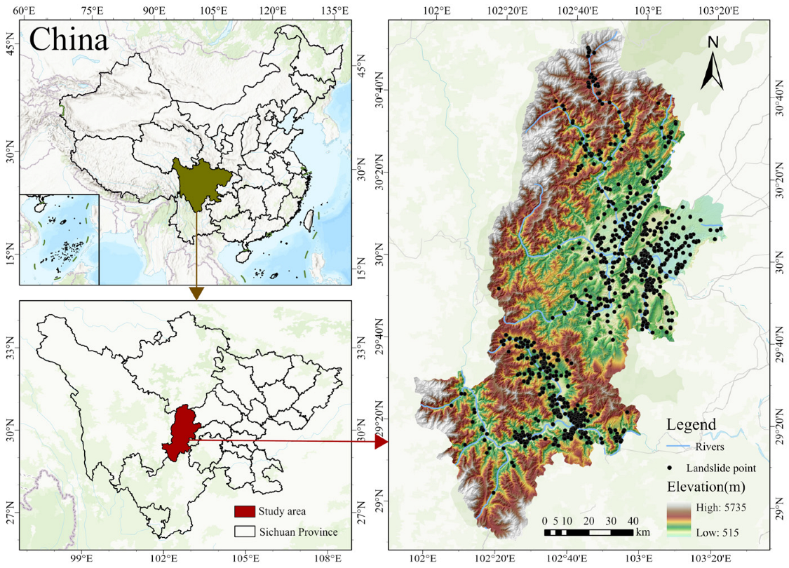
Figure 1. Location of the study area and spatial distribution of historical landslide points.
Land 14 01472 g001
Figure 2. Landslide influencing factors. (a) elevation, (b) slope, (c) aspect, (d) the topographic wetness index (TWI), (e) profile curvature, (f) plane curvature, (g) surface roughness, (h) the Normalized Difference Vegetation Index (NDVI), (i) prediction, (j) lithology, (k) distance to faults, (l) landuse, (m) distance to roads, (n) distance to rivers, (o) soil.
Land 14 01472 g002
Figure 3. Technical roadmap.
Land 14 01472 g003
Figure 4. The structure of the U-Net model.
Land 14 01472 g004
Figure 5. Correlation of landslide influencing factors.
Land 14 01472 g005
Figure 6. Feature importance of landslide influencing factors.
Land 14 01472 g006
Figure 7. Distribution of affiliation value and cumulative percentage curve of landslides.
Land 14 01472 g007
Figure 8. Landslide susceptibility map based on SFCM.
Land 14 01472 g008
Figure 9. Model performance analysis using ROC curves under different sampling strategies: (a) CNN, (b) U-Net and (c) SVM.
Land 14 01472 g009
Figure 10. Prediction rate curves of different models under various sampling methods: (a) CNN, (b) U-Net and (c) SVM.
Land 14 01472 g010
Figure 11. (ai) Landslide susceptibility zoning maps.
Land 14 01472 g011
Figure 12. FCM membership distribution and associated landslide cumulative curve.
Land 14 01472 g012
Figure 13. Landslide susceptibility zonation result based on FCM.
Land 14 01472 g013
Table 1. Data information of this study.
DataSourcesResolution
ElevationGeospatial Data Cloud Platform (http://www.gscloud.cn, accessed on 1 June 2024)30 m
Geological faultsGeological Cloud Platform (https://geocloud.cgs.gov.cn, accessed on 1 June 2024)1:1,000,000
LithologyNational 1:200,000 digital geological map (https://geocloud.cgs.gov.cn, accessed on 1 June 2024)1:200,000
NDVINational Ecosystem Science Data Center (http://www.nesdc.org.cn, accessed on 1 June 2024)30 m
Land useChina Land Cover Dataset (CLCD) (https://zenodo.org/records/12779975, accessed on 1 June 2024)30 m
SoilSoil map of the People’s Republic of China (https://www.resdc.cn, accessed on 1 June 2024)1:1,000,000
RoadNational Basic Geographic Database (https://www.webmap.cn, accessed on 1 June 2024)1:1,000,000
RiverNational Basic Geographic Database (https://www.webmap.cn, accessed on 1 June 2024)1:1,000,000
PrecipitationSichuan Meteorological Bureau-
Table 2. Frequency ratio of landslide influencing factor classification.
FactorsCategoryFRCategoryFR
Elevation (m)<13003.012700–35000.07
1300–20000.95>35000.00
2000–27000.16
Aspect (°)<1060.94250–2880.97
106–1421.04>2880.84
142–2501.17
Slope (°)0–151.9035–480.32
15–281.4348–550.11
28–350.48>550.23
Plane curvature<−3.20.000.5–3.30.65
−3.2–−0.80.67>3.30.18
−0.8–0.51.33
Profile curvature<−2.50.200.5–2.90.95
−2.5–−0.40.78>2.90.53
−0.4–0.51.36
Surface roughness<1.21.361.7–2.80.20
1.2–1.30.29>2.80.00
1.3–1.70.24
TWI<5.20.7615.7–22.62.97
5.2–12.51.21>22.63.66
12.5–15.71.35
LithologyUrban0.15Basalt0.94
Metamorphic rock0.11Granite0.95
Continental deposit0.54Lake6.45
Clastic rock1.92Outcrop0.00
Carbonatite1.04
Distance to faults (m)<20000.718000–12,0002.00
2000–50000.9112,000–16,0001.33
5000–80001.35>16,0000.51
NDVI<0.20.290.5–0.71.07
0.2–0.41.05>0.70.68
0.4–0.51.55
Land useCropland4.72Water0.81
Forest0.48Snow/Ice0.00
Shrub0.41Barren0.00
Grassland0.19Impervious1.92
SoilLeached soil0.29Alpine Soil0.00
Semi-leached soil0.00Pedalfer0.90
Primitive Soil2.62Rock0.00
Half-Hydromorphic Soil0.00Glacial Snow Cover0.00
Anthropic Soil2.80
Distance to roads (m)<5003.312500–35000.88
500–15001.613500–45000.50
1500–25001.06>45000.30
Precipitation (mm)<11000.781500–16003.07
1100–13000.38>16003.93
1300–15002.47
Distance to rivers (m)<10002.744000–50000.90
1000–20002.125000–60000.61
2000–30001.49>60000.33
3000–40001.01
Table 3. Multi-collinearity analysis of landslide factors.
FactorsVIFTOL
Elevation3.780 0.265
Aspect1.013 0.987
Slope6.084 0.164
Surface roughness4.686 0.213
Profile curvature1.764 0.567
Plane curvature1.759 0.569
Distance to faults1.151 0.868
NDVI1.222 0.818
Precipitation1.727 0.579
TWI1.335 0.749
Lithology1.624 0.616
Land use1.663 0.601
Soil2.158 0.463
Distance to rivers1.379 0.725
Distance to roads1.734 0.577
Table 4. Evaluation of landslide susceptibility assessment models.
Sampling StrategyModelAccuracy (%)Precision (%)Recall (%)F1 Score (%)Specificity (%)
LSI-SFCMCNN0.895 0.877 0.8810.879 0.906
U-Net0.9020.895 0.877 0.8860.921
SVM0.882 0.8980.859 0.878 0.904
SFCMCNN0.878 0.897 0.815 0.854 0.927
U-Net0.8840.890 0.8370.8630.920
SVM0.850 0.9010.794 0.844 0.909
RSCNN0.8200.7670.8460.8050.800
U-Net0.815 0.761 0.840 0.799 0.795
SVM0.772 0.747 0.818 0.781 0.727
Table 5. Area proportion statistics of different landslide susceptibility zones.
Sample
Selection
ModelArea Percentage (%)
Very LowLowModerateHighVery High
LSI-SFCMCNN50.2918.438.146.3716.77
U-Net50.1718.469.635.8515.90
SVM21.4544.0113.179.5711.80
SFCMCNN64.3611.644.874.9214.20
U-Net59.3413.908.116.1512.50
SVM6.3566.236.356.5814.48
RSCNN60.99 14.285.8910.738.12
U-Net61.6213.248.7910.445.91
SVM3.4167.238.3412.208.82
Table 6. Landslide proportion statistics in different landslide susceptibility zones.
Sample
Selection
ModelLandslides Percentage (%)
Very LowLowModerateHighVery High
LSI-SFCMCNN1.674.065.5111.3977.37
U-Net1.523.778.7010.0175.78
SVM0.804.218.5612.3374.11
SFCMCNN4.355.877.6911.7570.34
U-Net2.904.869.4315.9566.86
SVM0.2917.693.3410.3068.38
RSCNN3.637.476.9628.2153.73
U-Net3.057.0311.3935.1743.36
SVM0.0716.246.6030.1746.92
Disclaimer/Publisher’s Note: The statements, opinions and data contained in all publications are solely those of the individual author(s) and contributor(s) and not of MDPI and/or the editor(s). MDPI and/or the editor(s) disclaim responsibility for any injury to people or property resulting from any ideas, methods, instructions or products referred to in the content.