Abstract
This study focuses on the Dongting Lake region in China and evaluates ecological vulnerability using the Sensitivity–Resilience–Pressure (SRP) framework, integrated with Spatial Principal Component Analysis (SPCA) to calculate the Ecological Vulnerability Index (EVI). The EVI values were classified into five levels using the Natural Breaks (Jenks) method, and spatial autocorrelation analysis was applied to reveal spatial differentiation patterns. The Geodetector model was used to analyze the driving mechanisms of natural and socioeconomic factors on EVI, identifying key influencing variables. Furthermore, the LightGBM algorithm was used for feature optimization, followed by the construction of six machine learning models—Multilayer Perceptron (MLP), Extremely Randomized Trees (ET), Decision Tree (DT), Random Forest (RF), LightGBM, and K-Nearest Neighbors (KNN)—to conduct multi-class classification of ecological vulnerability. Model performance was assessed using ROC–AUC, accuracy, recall, confusion matrix, and Kappa coefficient, and the best-performing model was interpreted using SHAP (SHapley Additive exPlanations). The results indicate that: ① ecological vulnerability increased progressively from the core wetlands and riparian corridors to the transitional zones in the surrounding hills and mountains; ② a significant spatial clustering of ecological vulnerability was observed, with a Moran’s I index of 0.78; ③ Geodetector analysis identified the interaction between NPP (q = 0.329) and precipitation (PRE, q = 0.268) as the dominant factor (q = 0.50) influencing spatial variation of EVI; ④ the Random Forest model achieved the best classification performance (AUC = 0.954, F1 score = 0.78), and SHAP analysis showed that NPP and PRE made the most significant contributions to model predictions. This study proposes a multi-method integrated decision support framework for assessing ecological vulnerability in lake wetland ecosystems.
1. Introduction
As a key ecological security barrier in the middle reaches of the Yangtze River and a wetland of international importance, the Dongting Lake region plays a critical role in maintaining biodiversity and supporting the sustainable development of the Yangtze River Economic Belt. In recent years, under the compound stress of climate change, land reclamation, and hydraulic engineering, the region has faced increasingly severe ecological issues, including wetland degradation and disrupted hydrological regimes, leading to significantly heightened ecological vulnerability [1,2,3]. Scientifically assessing the spatial heterogeneity of ecological vulnerability and accurately identifying its driving mechanisms has become a pressing need in implementing the strategy of “ecological priority and green development” in the Yangtze River Economic Belt.
Numerous methods for evaluating ecological vulnerability have been proposed in recent years. Among them, the Ecological Vulnerability Index (EVI) based on the Sensitivity–Resilience–Pressure (SRP) model has gained widespread adoption due to its scientific rigor and practical applicability [4,5,6,7]. By integrating sensitivity factors, resilience indicators, and pressure drivers, the SRP model effectively captures the vulnerability of ecological systems. Its validity has been confirmed in various regions such as the Yellow River Basin and the Loess Plateau [8,9]. Given the high-dimensional nature of EVI calculation, Spatial Principal Component Analysis (SPCA) has been increasingly used as a dimensionality reduction technique. It not only extracts key information but also mitigates multicollinearity among variables while preserving essential data characteristics [10,11,12]. In the SRP framework, the choice of classification method is equally important. The Natural Breaks (Jenks) method, a widely used unsupervised classification technique, automatically determines threshold values based on intrinsic data characteristics, thereby avoiding subjective bias [13,14]. To further analyze spatial differentiation, spatial autocorrelation techniques, including global Moran’s I and local indicators of spatial association (LISA) clustering, are frequently employed. These methods help identify the spatial clustering and hot–cold spot patterns of ecological vulnerability [15,16,17,18].
Following ecological vulnerability assessment, it is crucial to identify the driving forces. Traditional evaluations often rely on static indicators and linear assumptions, which may fail to capture the complex and nonlinear interactions among environmental, climatic, and socioeconomic factors. The emerging Geodetector technique addresses this limitation by offering novel methodological tools for identifying ecological drivers through factor detection and interaction detection [19,20]. It has demonstrated significant advantages in landscape ecological risk assessment and vegetation dynamics research [21,22,23], enabling robust identification of dominant and synergistic influencing factors.
The rapid advancement of Machine Learning algorithms has provided new opportunities for ecological vulnerability classification. Algorithms such as LightGBM have shown excellent performance in both feature optimization and model construction [24,25]. Various multi-class models, including Multilayer Perceptron (MLP), Random Forest (RF), and K-Nearest Neighbors (KNN), have been widely applied in ecological studies [26,27,28], particularly for handling high-dimensional, nonlinear data. However, the lack of interpretability remains a major limitation. To address this, the SHAP (SHapley Additive exPlanations) method has been introduced to interpret the decision-making processes of models. Based on cooperative game theory, SHAP quantitatively measures feature contributions, offering transparent decision support in water quality prediction, ecological assessment, and integrated disaster risk analysis [29,30,31].
This study takes the Dongting Lake region as the study area and integrates the SRP model, SPCA, Geodetector, and Machine Learning techniques to achieve the following objectives:
- (1)
- calculate the EVI based on the SRP model and classify ecological vulnerability levels;
- (2)
- explore the spatial heterogeneity of EVI and investigate its natural and socioeconomic drivers;
- (3)
- perform feature selection and construct six multi-class Machine Learning models (MLP, ET, DT, RF, LightGBM, KNN), identify the most efficient and cost-effective model, and interpret it using the SHAP framework.
This research aims to provide a scientific foundation for ecological protection and restoration in the Dongting Lake region and explore the applicability of Machine Learning approaches in ecological vulnerability assessment.
2. Materials and Methods
2.1. Study Area Overview
The Dongting Lake region (28°10′–30°10′ N, 111°30′–113°50′ E) is located in the north-central part of Hunan Province, China. It serves as both a wetland ecosystem of international importance and a key ecological barrier in the Yangtze River Basin. The study area encompasses the administrative territories of Yueyang, Yiyang, and Changde, with a total area of approximately 37,267 km2 (Figure 1). The region is centered around Dongting Lake, featuring a dense river network fed by major tributaries such as the Xiangjiang, Zishui, Yuanjiang, and Lishui Rivers.
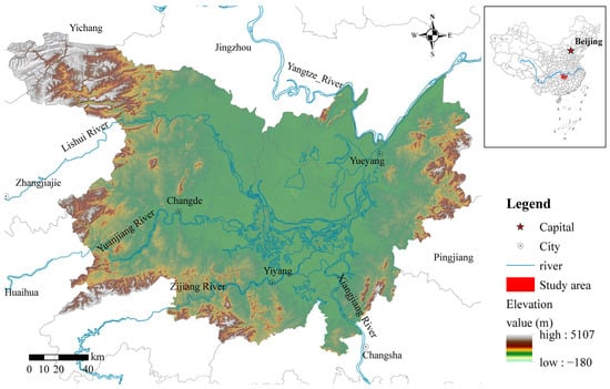
Figure 1.
Geographical location of the Dongting Lake region.
Geomorphologically, the lake basin forms a horseshoe-shaped depression, open to the north, surrounded by the Wuling Mountains to the west, the Xuefeng Mountains to the south, and the Mufu Mountains to the east. This topographic configuration creates a landscape described as “enclosed on three sides by mountains and open to the Yangtze River in the north.”
The region exhibits a subtropical monsoon climate, characterized by four distinct seasons. The mean annual precipitation ranges from 1200 to 1500 mm, with rainfall predominantly occurring during the summer and autumn months. The average annual temperature is approximately 16–17 °C. The warm and humid climatic conditions provide favorable circumstances for vegetation growth and ecological succession in the Dongting Lake area. Moreover, the wetland ecosystems in this region play a vital role in regulating water levels and stabilizing the climate within the broader Yangtze River Basin.
2.2. Data Sources and Processing
To accurately assess ecological vulnerability in the Dongting Lake region, this study focused on collecting both natural environmental and socioeconomic indicators. A total of 14 variables were selected, with detailed sources listed in Table 1. To ensure spatial consistency and alignment across datasets, all raw data were projected to the CGCS2000 111° zone coordinate system using ArcGIS 10.8.2 and Python 3.10.8. Further preprocessing steps included filling missing values, clipping to the study area, and resampling. All raster data were standardized to a spatial resolution of 500 m.

Table 1.
Ecological vulnerability assessment indicators, data sources, and resolution.
2.3. Methodology
2.3.1. Technical Framework
This study consisted of four main steps. First, an evaluation indicator system was constructed based on the Sensitivity–Resilience–Pressure (SRP) framework by selecting 14 indicators representing natural environmental and socioeconomic factors. Second, Spatial Principal Component Analysis (SPCA) was applied to reduce dimensionality, retaining principal components that, together, explained over 85% of the total variance. These components were used to calculate the Ecological Vulnerability Index (EVI) based on their respective weights. Subsequently, global and local spatial autocorrelation of EVI was analyzed using Moran’s I to identify spatial clustering patterns.
Third, the Geodetector model was employed to perform both single-factor and interaction detection on the 14 indicators to explore the driving mechanisms of ecological vulnerability in the Dongting Lake region. Finally, the LightGBM algorithm was introduced for feature selection. Based on the selected features, multiple Machine Learning models for multi-class ecological vulnerability classification were constructed, including hyperparameter tuning and model performance evaluation. The optimal model was then interpreted using the SHAP method to identify the contribution of each selected variable. The complete technical framework is illustrated in Figure 2.
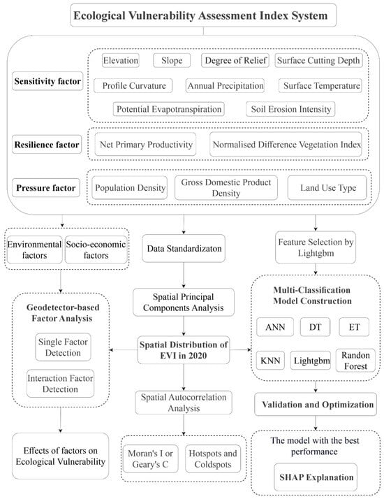
Figure 2.
Flowchart of ecological vulnerability assessment and analysis in the Dongting Lake region.
2.3.2. Construction of the Ecological Vulnerability Assessment System
The selection of evaluation indicators is a complex process. In this study, an ecological vulnerability assessment system was developed based on the SRP model, with consideration of the ecological and environmental characteristics of the Dongting Lake region. The indicator selection followed the principles of scientific validity, comprehensiveness, representativeness, and the integration of qualitative and quantitative approaches, aiming to holistically reflect the regional ecological conditions [32,33]. A total of 14 indicators were selected under two broad categories—natural environment and socioeconomic factors—encompassing terrain, land ecology, climate, and human activity. The indicators and their spatial distribution are shown in Table 1 and Figure 3.
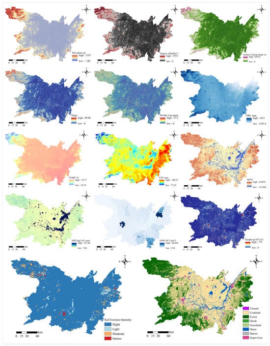
Figure 3.
Spatial distribution of each indicator.
Ecological sensitivity refers to the degree to which an ecosystem responds to external environmental changes and is a critical component of ecological vulnerability assessment. Areas with higher sensitivity are more prone to ecological degradation when disturbed. In this study, nine indicators were selected to quantify ecological sensitivity: elevation of digital elevation model (DEM), slope, profile curvature (PCV), degree of relief (DR), surface cutting depth (SCD), soil erosion intensity (SEI), annual precipitation (PRE), land surface temperature (TEMP), and potential evapotranspiration (EVT).
Ecological resilience describes the ability of an ecosystem to self-regulate and recover following disturbances. Two indicators were chosen to represent this dimension: net primary productivity (NPP) and the normalized difference vegetation index (NDVI). Both effectively capture vegetation growth and recovery capacity in the study region.
Ecological pressure refers to the intensity of external stresses on ecosystems, primarily from socioeconomic activities and human interventions. This study selected gross domestic product density (GDP), population density (POP), and land use types (LUT) as proxies for ecological pressure, reflecting both anthropogenic and economic impacts.
The interactions among these indicators are complex. Specifically, higher ecological sensitivity and pressure levels are generally associated with increased ecological vulnerability, while greater resilience tends to mitigate vulnerability. A comprehensive analysis of these indicators enables a systematic assessment of the ecological status in the study area.
2.3.3. Index Data Standardization
To eliminate dimensional inconsistencies and directional heterogeneity among multi-source data, a standardized and comparable indicator matrix was constructed using two standardization strategies based on indicator attributes:
- (1)
- Quantitative indicators were standardized using the dynamic range method [34], which retains the original distribution characteristics of the data:
Positive indicators (positively correlated with vulnerability) were normalized using:
Negative indicators (negatively correlated with vulnerability) were normalized using:
where, and represent the standardized values of the positive and negative indicator ; denotes the original value of the indicator ; and and refer to the maximum and minimum values of the indicator .
- (2)
- Qualitative indicators, such as land use type and soil erosion intensity, were normalized based on expert scoring and literature-based classification schemes. The standardized values are shown in Table 2.
Table 2. Standardized values of land use types and soil erosion intensity.
2.3.4. Spatial Principal Component Analysis (SPCA)
To address spatial autocorrelation among multidimensional ecological indicators, Spatial Principal Component Analysis (SPCA) was applied to the 14 standardized indicators to decouple spatial dependencies. Unlike traditional PCA, SPCA introduces a kernel density-based spatial weight matrix to incorporate spatial heterogeneity in the dimensionality reduction process [35].
The SPCA was performed via singular value decomposition (SVD) of the correlation coefficient matrix, resulting in 14 principal components. Based on the criterion of accumulated variance contribution ≥ 85%, the first five components (PC1–PC5) were retained as composite variables. These components effectively preserve the core information of the original indicators, reduce data redundancy, and eliminate multicollinearity, thereby enhancing the accuracy and interpretability of ecological vulnerability assessments.
The comprehensive Ecological Vulnerability Index (EVI) was computed using:
where is the weight of the i-th principal component, is the score of the i-th component, and is the number of selected components.
The results of the SPCA are presented in Table 3, and the analysis was conducted using ArcGIS 10.8.
Table 3.
SPCA results of ecosystem vulnerability in the Dongting Lake region.
2.3.5. Classification of the Ecological Vulnerability Index (EVI)
To objectively classify the Ecological Vulnerability Index (EVI), this study employed the Natural Breaks Classification (NBC) method to statistically categorize EVI values for the Dongting Lake region in 2020 [36]. This method identifies natural gaps in the data distribution to establish classification thresholds, allowing the division of ecological vulnerability into five levels: slight vulnerability, light vulnerability, medium vulnerability, heavy vulnerability, and extreme vulnerability.
The primary advantage of NBC lies in its ability to maximize within-class homogeneity and between-class heterogeneity by identifying optimal breakpoints based on the intrinsic distribution of the data. This approach effectively reduces subjective bias associated with manually defined thresholds, ensuring greater statistical objectivity and classification accuracy.
2.3.6. Spatial Autocorrelation Analysis
To explore spatial relationships of EVI, global and local spatial autocorrelation analyses were conducted using ArcGIS 10.8. Given that geographic elements typically exhibit spatial dependency, Moran’s I was employed to assess global clustering tendencies [37,38], calculated as:
where and represent EVI values in spatial units and ; is the spatial weight between units; and is the mean. Significance testing was performed using Z-scores and p-values. A significantly positive Moran’s I indicates strong spatial clustering, while a negative value reflects dispersion.
Local Indicators of Spatial Association (LISA) were used to identify spatial heterogeneity patterns such as High–High clusters (vulnerability hotspots) and Low–Low clusters (stable zones). This dual-scale approach enhances spatial interpretability and provides insights for localized vulnerability mitigation.
2.3.7. Factor Analysis Using the Geodetector Model
The Geodetector model was employed in conjunction with Python scripting to automate the analysis of large-scale spatial data and uncover the driving mechanisms of EVI spatial heterogeneity [39,40]. The model quantifies the independent and interactive effects of the 14 selected indicators on ecological vulnerability.
Gridded pixels were used as extraction units, linking the 14 indicators as independent variables and the EVI as the dependent variable. To manage data scale, continuous variables were discretized into five classes using the jenkspy library (Figure 4).
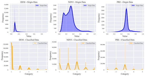
Figure 4.
Comparison of data before and after natural breaks classification for typical indicators.
The q-statistic of each factor was calculated using:
where is the number of strata, and are the sample size and variance within stratum , and and are the total sample size and variance. The q-value ranges from 0 to 1, indicating the explanatory power of each factor on EVI spatial variation.
For interaction detection, pairs of variables were tested to assess their combined explanatory power, identifying synergistic or nonlinear effects. These results, ranked by explanatory strength, provide a deeper understanding of how factor combinations influence spatial vulnerability distributions.
2.3.8. Feature Selection and Machine Learning Model
Using ArcGIS raster analysis and point value extraction, all 14 standardized indicators (feature variables) were spatially linked to the EVI classification (target variable) to construct the dataset. This was done based on a grid resolution of 500 m × 500 m, and the indicators were treated as continuous variables.
Given the class imbalance in EVI categories, a 1 km × 1 km stratified sampling approach was applied to oversample the underrepresented classes. Compared to the traditional random sampling method, this technique better preserves the original data characteristics and spatial uniformity of oversampled categories. The dataset was then split into training and testing sets using a 7:3 ratio, resulting in 43,433 training samples and 18,615 testing samples.
A LightGBM model was built and evaluated using 5-fold cross-validation. The Area Under the Curve (AUC) was calculated for each fold and averaged to assess model performance. Feature importance scores were extracted for the 14 indicators, and features were sequentially added based on descending importance to iteratively construct models with varying numbers of features. A feature–AUC curve was plotted to identify the optimal feature subset that maximizes model performance while ensuring parsimony. This feature selection process aimed to optimize model efficiency and accuracy [41,42].
Based on this analysis, eight key indicators (PRE, NPP, ETP, NDVI, GDP, TEMP, DEM, and LUT) were selected to reconstruct the classification models while retaining as many categorical features as possible (Figure 5).
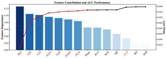
Figure 5.
Relationship between feature contribution and the AUC performance of LightGBM.
- ①
- Multilayer Perceptron (MLP)
MLP is a classic deep learning model composed of an input layer, one or more hidden layers, and an output layer. It captures nonlinear and complex relationships through multiple transformation layers. In ecological vulnerability classification, MLP effectively learns the mapping between multidimensional environmental features and vulnerability categories, delivering high prediction accuracy.
- ②
- Decision Tree (DT)
DT is a tree-based algorithm that recursively splits the feature space into decision regions. Each leaf node represents a predicted class. It is highly interpretable and well-suited for classification problems.
- ③
- Extra Trees (ET)
Extra Trees is an ensemble learning algorithm that builds multiple decision trees while introducing randomness in both feature selection and split thresholds. Compared to conventional decision trees, ET offers faster training, better generalization, and reduced overfitting.
- ④
- K-Nearest Neighbors (KNN)
KNN is a non-parametric method that classifies instances based on similarity in feature space. For each test sample, the Euclidean distance to training samples is calculated, and the 7 nearest neighbors are identified (k = 7). The class label is determined by majority voting. KNN is particularly effective for high-dimensional data and requires no explicit model training.
- ⑤
- Light Gradient Boosting Machine (LightGBM)
LightGBM is a highly efficient gradient boosting algorithm that uses histogram-based algorithms for faster feature splits. It supports categorical variables and missing value handling, with low memory consumption, making it ideal for large-scale geospatial data.
- ⑥
- Random Forest (RF)
RF is another ensemble method based on bagging. It generates multiple decision trees using bootstrap samples and aggregates their results through majority voting (classification). This approach improves model robustness and generalization by reducing variance.
In this study, a distinct set of hyperparameters was defined for each of the six Machine Learning models. To optimize these parameters automatically, the GridSearchCV module within the Scikit-learn framework was employed.
A nested 5-fold cross-validation procedure was implemented to ensure robust and unbiased model selection. During each parameter iteration, the training set was randomly partitioned into five mutually exclusive folds. In each round, four folds were used for training and the remaining fold for validation, such that every fold was used once as the validation set.
The macro-F1 score was adopted as the evaluation criterion, and the hyperparameter configuration that achieved the highest macro-F1 score across the validation folds was selected as optimal. This nested strategy effectively reduces the risk of bias introduced by a single train–test split and ensures that the selected parameters exhibit strong generalization performance on unseen data.
2.3.9. Evaluation Metrics for Classification Models and SHAP-Based Interpretation
To evaluate the classification performance of the Machine Learning models, several commonly used metrics were employed:
- ①
- Accuracy:
Accuracy is defined as the ratio of correctly classified samples to the total number of samples, reflecting the overall performance of the model.
- ②
- Precision:
Precision is the ratio of true positive predictions to all predicted positives. It reflects the model’s ability to correctly identify positive classes.
- ③
- Recall (Sensitivity):
Recall is the ratio of correctly predicted positive instances to all actual positive instances, measuring the model’s coverage of true positive samples.
- ④
- F1 Score:
The F1 score is the harmonic mean of precision and recall. It provides a balanced evaluation of a classifier, particularly under imbalanced class distributions.
- ⑤
- ROC–AUC (Receiver Operating Characteristic–Area Under the Curve):
The ROC–AUC curve plots the true positive rate (TPR) against the false positive rate (FPR). The AUC value measures the classifier’s ability to distinguish between classes. An AUC closer to 1.0 indicates superior performance.
In this study, a One-vs-Rest (OvR) strategy was used to compute the macro-average AUC in the multiclass setting. An AUC > 0.90 was considered indicative of excellent classification performance. All other evaluation metrics were also macro-averaged across classes.
Definitions:
TP: true positives.
TN: true negatives.
FP: false positives.
FN: false negatives.
- ⑥
- Cohen’s Kappa Coefficient:
Kappa measures the overall agreement between the predicted and actual classifications, adjusted for chance agreement. It ranges from −1 to 1, where values above 0.6 are generally considered to indicate substantial consistency.
where represents the number of samples located on the i-th row and i-th column of the confusion matrix; n is the total number of classes; denotes the total number of samples used for accuracy evaluation; and are the total number of samples in the i-th row and i-th column.
- ⑦
- SHAP (SHapley Additive exPlanations):
SHAP is an explainable Machine Learning framework based on cooperative game theory, particularly the Shapley value. It quantifies the contribution of each feature to the model’s prediction.
The prediction output of a Machine Learning model can be decomposed as:
where is the model prediction for sample , is the baseline value (mean prediction across all samples), and is the Shapley value of the i-th feature, representing its marginal contribution to the prediction.
The SHAP framework provides both local and global interpretability. Local interpretation explains individual predictions by visualizing sample-level contribution heatmaps, identifying key factors driving the outcome. Global interpretation aggregates SHAP values across samples to assess overall feature importance and the direction of influence [43,44].
3. Results
3.1. Spatial Differentiation Patterns of Ecological Vulnerability
In 2020, the ecological vulnerability in the Dongting Lake region exhibited a distinct gradient pattern, with EVI values ranging from 0.29 to 1.14. Five levels of ecological vulnerability—slight, light, medium, heavy, and extreme—were identified using the Natural Breaks Classification method (Table 4, Figure 6).
Table 4.
Area and proportion of different ecological vulnerability levels in the Dongting Lake region in 2020.
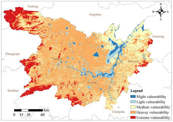
Figure 6.
Spatial distribution of ecological vulnerability in the Dongting Lake region.
The low-vulnerability core areas, namely the slight and light vulnerability zones, covered relatively small areas of 1144.78 km2 and 1760.31 km2, accounting for 3.07% and 4.72% of the total area, respectively. These zones were mainly concentrated in the central water body of Dongting Lake and along buffer strips of major rivers such as the Xiang River and Zishui River. Benefiting from hydrological regulation by wetlands, these areas exhibited better vegetation coverage, experienced less human disturbance than surrounding zones, and maintained a relatively stable ecosystem.
The medium vulnerability zone covered 8242.26 km2, accounting for 22.12% of the total area. It was primarily distributed in the eastern and northeastern parts of the lake region along the southern bank of the Yangtze River, with scattered patches in the west. This zone was under moderate ecological pressure due to seasonal hydrological fluctuations, intensive agricultural practices, and stress from low-mountain forest lands. However, overall ecological functions remained sustainable.
The high-vulnerability expansion areas—comprising the heavy and extreme vulnerability zones—covered 21,943.19 km2 and 4176.47 km2, accounting for 58.88% and 11.21%, respectively. The heavy vulnerability zone was the most extensive, widely distributed across the central-western parts of the region, particularly in Changde and Yiyang. This area corresponds to the former West Dongting Lake, where land reclamation and urban expansion have caused significant shrinkage of natural wetlands, rendering the ecosystem more susceptible to external disturbances. Extreme vulnerability areas appeared in fragmented patches, mostly located along the southern slopes of the Xuefeng Mountains in the west and the residual ridges of the Mufu Mountains in the east. Rugged terrain, steep-slope cultivation, and mining relics compounded the ecological fragility, limiting restoration potential and resulting in low ecological resilience.
Overall, ecological vulnerability in the Dongting Lake region displays a complex spatial differentiation pattern with notable inter-regional disparities. In particular, the distribution of heavy and extreme vulnerability zones reflects the combined influence of human activities and natural conditions. Targeted and region-specific ecological restoration and protection strategies should be implemented based on the vulnerability characteristics of each zone.
3.2. Spatial Autocorrelation Characteristics of Ecological Vulnerability
This study employed spatial autocorrelation models to reveal the spatial dependency pattern of ecological vulnerability in the Dongting Lake region. The Global Moran’s I index was calculated as 0.78 (Z = 425.68, p < 0.01), indicating a statistically significant positive spatial correlation. This suggests that adjacent areas exhibit similar levels of vulnerability, demonstrating a strong degree of spatial dependency and a highly clustered distribution (Figure 7a).
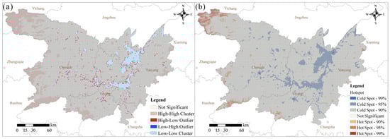
Figure 7.
LISA and Getis-Ord Gi* analysis of ecological vulnerability in the Dongting Lake region: Local Indicators of Spatial Association cluster analysis (a); Getis–Ord Gi* hotspot analysis (b).
Based on Local Indicators of Spatial Association (LISA) cluster analysis, four spatial association patterns were identified (Figure 7b). High–High clusters were mainly concentrated in the western region of the lake, particularly along the Wuling Mountain foothills, the peak-cluster area of the Xuefeng Mountains in the southwest, and the low slopes of the Mufu Mountains in the east. These zones exhibited significantly higher average EVI values and terrain ruggedness, forming key sources of ecological vulnerability diffusion.
Low–Low clusters were centered around the Dongting Lake water body and extended in a belt-like pattern along the main courses of the Xiang and Yuan rivers. These zones had the highest NDVI averages and wetland coverage rates, coupled with relatively low human disturbance indices, indicating ecological stability cores.
High–Low and Low–High (LH) transitional clusters were sporadically distributed in the lake–mountain transition zones and buffer regions along major tributaries.
Getis–Ord Gi* hotspot analysis (99% confidence level) further revealed significant spatial clustering of both hotspot and coldspot areas. Hotspots were spatially coupled with HH clusters and covered areas such as the Xuefeng and Mufu Mountains, which represent regions with extreme ecological vulnerability. These hotspots play a dominant role in shaping the overall spatial pattern of vulnerability. In contrast, coldspots were mainly distributed in the lake center and confluence zones of major rivers, reflecting the stabilizing effect of wetland ecosystems in suppressing the spread of ecological vulnerability.
3.3. Factor Driving Analysis Using Geodetector
3.3.1. Results of Single-Factor Detection
Based on the Geodetector model, all 14 selected driving factors passed the significance test (p = 0), indicating that each contributes to the spatial differentiation of ecological vulnerability in the Dongting Lake region. However, the explanatory power of these factors exhibited a clear gradient of variation (Figure 8).
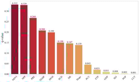
Figure 8.
Sorting of q-values for the single-factor detection of ecological vulnerability in the Dongting Lake region.
Among them, NDVI, NPP, PRE, TEMP, and DEM emerged as the dominant driving factors, with q-values of 0.332, 0.329, 0.268, 0.208, and 0.199. These results suggest that natural factors—particularly vegetation resilience, hydrothermal conditions, and topography—play a major role in shaping ecological vulnerability patterns across the study area.
In contrast, GDP, SEI, POP, and LUT were found to be weaker explanatory factors, with q-values all below 0.011. This implies that while socioeconomic and anthropogenic stressors contribute to ecological vulnerability, their influence is relatively limited in comparison to natural environmental variables in the Dongting Lake context.
3.3.2. Results of Interaction Detection
The interaction analysis using the Geodetector model indicates that the spatial differentiation of ecological vulnerability in the Dongting Lake region is primarily governed by nonlinear synergistic effects among multiple factors. The interaction explanatory power (q-values) of all factor combinations significantly exceeded those of individual factors, highlighting the amplifying role of factor interplay.
The dominant interaction types were nonlinear enhancement and bilinear enhancement, and the explanatory power of leading interaction combinations exhibited clear hierarchical variation. Notably, the combinations of NPP ∩ PRE, NPP ∩ TEMP, NPP ∩ DEM, and NDV ∩ PRE demonstrated the highest explanatory power, with q-values approaching 0.5 (Figure 9). These results emphasize the strong coupling between vegetation productivity and climatic or topographic conditions, which is essential for maintaining ecosystem stability and mitigating ecological vulnerability across the Dongting Lake basin.
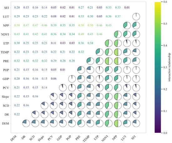
Figure 9.
Interaction analysis of ecological vulnerability factors in the Dongting Lake region.
Moreover, other interaction pairs also exhibited considerable enhancement effects, further reinforcing the collective explanatory capacity of the driving factors and jointly shaping the spatial distribution of ecological vulnerability.
In summary, ecological vulnerability in the Dongting Lake region is not merely the result of individual driving factors but rather a complex manifestation of multi-factor interactions. These interactions exert a significant magnifying influence on spatial heterogeneity and should be comprehensively considered in the formulation of ecological protection and management strategies.
3.4. Evaluation of Multi-Class Ecological Vulnerability Models
To explore a more efficient and cost-effective method for classifying ecological vulnerability levels, this study systematically constructed six classification models—Artificial Neural Network (ANN), Decision Tree (DT), Extra Trees (ET), K-Nearest Neighbors (KNN), LightGBM, and Random Forest (RF)—based on the eight key indicators selected in Section 2.3.8. Under rigorous five-fold cross-validation and a macro-averaged evaluation framework, the models demonstrated significant performance variability.
According to the macro-averaged ROC–AUC evaluation, ensemble learning models showed clear superiority in capturing nonlinear boundaries and high-order interactive effects in ecological vulnerability classification. RF, ET, and LightGBM all achieved an AUC value of 0.954, forming the top-performing tier and outperforming DT, KNN, and ANN (Figure 10a). Across conventional classification metrics, all models exhibited convergence, with macro-averaged accuracy, precision, recall, and F1-score ranging within 0.76 ± 0.02, reflecting the inherent complexity of vulnerability level classification. The Kappa coefficient (0.70 ± 0.02) further confirmed strong consistency between the predicted and actual classifications. Among all models, Random Forest performed best, achieving an F1-score and accuracy of 0.78, with a Kappa coefficient of 0.71, indicating substantial agreement (Figure 10b).
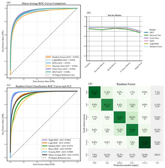
Figure 10.
Presentation of evaluation metrics for Machine Learning models.
To further assess category-level prediction performance, the Random Forest model—selected based on its superior macro-AUC and F1-score—was used to generate ROC–AUC curves and a confusion matrix for each ecological vulnerability class (Figure 10c,d). The results showed that the AUC values for all five vulnerability classes exceeded 0.90, indicating high discriminative capacity. The extremely vulnerable class achieved the highest AUC at 0.990, followed closely by the slightly vulnerable class with 0.986. The AUC values for lightly, moderately, and heavily vulnerable classes were 0.956, 0.913, and 0.920, respectively, all reflecting strong classification performance.
The confusion matrix revealed that the prediction accuracies for the extremely and slightly vulnerable categories were 91.7% and 82.6%, respectively, highlighting the model’s robustness in identifying extreme ecological conditions. The moderately and heavily vulnerable classes were also predicted with relatively high accuracy (above 74%). In contrast, the lightly vulnerable class had the lowest prediction accuracy at 68.1%, indicating challenges in modeling transitional vulnerability states.
These results demonstrate that the constructed multi-class classification models are sufficiently accurate for identifying both extreme and low ecological vulnerability conditions. However, further refinement is needed to improve classification performance in intermediate zones, where ecological characteristics are often more complex and less distinguishable.
3.5. SHAP Interpretation of the Random Forest Model
To uncover the nonlinear driving mechanisms underlying ecological vulnerability classification, the SHAP framework was applied to the RF model. The global feature importance analysis (Figure 11a) indicated that NPP, PRE, LUT, and DEM were the dominant predictors of ecological vulnerability levels. In contrast, the explanatory power of the socioeconomic factor GDP was significantly lower than that of the natural variables, reaffirming the nature-dominated formation mechanisms of ecological vulnerability in the study area.
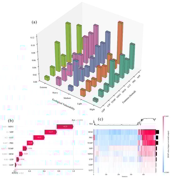
Figure 11.
Analysis of the driving factors for ecological vulnerability based on SHAP: The global feature importance analysis (a); local SHAP waterfall plot for the first correctly predicted slightly vulnerable sample (b); SHAP heatmap for the extremely vulnerable class (c).
At the class-specific level, slightly and lightly vulnerable regions were mainly influenced by NPP, LUT, and NDVI, suggesting that vegetation-related variables play a central role in maintaining low levels of vulnerability. In contrast, the extremely vulnerable category was predominantly controlled by PRE, DEM, and TEMP, underscoring the critical roles of climatic and topographic conditions in driving extreme ecological fragility.
To enhance interpretability and visualization, we further constructed a local SHAP waterfall plot for the first correctly predicted slightly vulnerable sample and an SHAP heatmap for the extremely vulnerable class (Figure 11b,c). The local SHAP waterfall plot illustrated that all eight indicators contributed positively to the prediction of slight vulnerability for this instance, with NDVI, NPP, and LUT acting as the primary drivers. The SHAP heatmap confirmed that DEM, PRE, and TEMP were the dominant predictors for the extremely vulnerable category.
In summary, the combined global and local SHAP analyses enabled a comprehensive identification of key drivers for each ecological vulnerability class. These results not only validate the relative importance of various predictors but also provide a deeper interpretive perspective for understanding the spatial heterogeneity of ecological vulnerability.
4. Discussion
4.1. Advantages and Limitations of the SRP Model
This study established an ecological vulnerability assessment framework for the Dongting Lake region based on the SRP model, integrating SPCA to compute the ecological vulnerability index. The SRP framework effectively captures the complexity of ecosystem vulnerability by combining natural sensitivity, ecological resilience, and anthropogenic pressure, thus overcoming the limitations of single-factor assessments. The SPCA retained five principal components with a cumulative variance contribution of 87.90%, demonstrating the efficiency of the SRP model in multi-source data integration.
However, in practical application, the selection and calculation methods of indicators in each SRP dimension (Sensitivity, Resilience, and Pressure) can significantly affect assessment outcomes. Despite employing SPCA for dimensionality reduction and data optimization, the model remains sensitive to the input data sources. The indicators used in this study to calculate vulnerability have been widely recognized as sensitive and responsive proxies of ecosystem status [45,46]. Nevertheless, we also acknowledge that potentially important ecological factors such as soil microbial activity and biodiversity were not included due to the lack of reliable spatial data at the regional scale, which may have introduced some bias into the results. Moreover, ecological vulnerability is inherently a dynamic process—driven by both climate change and human activities—where static assessments based on 2020 snapshot data cannot fully capture temporal dynamics [47,48]. The SRP model primarily reflects vulnerability under specific stressors, yet it does not explicitly account for self-regulation and adaptive capacities of ecosystems. This omission may lead to an overly pessimistic portrayal of ecological fragility.
Despite these limitations, the SRP-based assessment framework remains a valuable tool for uncovering the multi-factorial mechanisms and spatial heterogeneity of ecological vulnerability. Future improvements should consider integrating ecosystem service evaluations and time-series monitoring data, such as interannual water level fluctuations, to enhance the model’s capacity to capture spatiotemporal variations in vulnerability.
4.2. Evaluation Metrics and Challenges in Multi-Class Machine Learning Models
By comparing the classification performance of six Machine Learning models, this study highlights the complexity of evaluation metric selection in multi-class ecological tasks and the ecological implications of different metrics. Although all models achieved macro-average AUC values exceeding 0.90, conventional classification metrics such as accuracy and F1-score were generally below 0.80, with Kappa coefficients lower than 0.75. These discrepancies reflect the conflicts among evaluation perspectives and the unique classification challenges posed by ecological vulnerability gradations [49].
Two major factors account for this inconsistency:
- (1)
- Class ambiguity: Slightly and moderately vulnerable regions exhibit complex environmental characteristics influenced by multiple overlapping factors, making it difficult for models to delineate clear boundaries, thus lowering classification accuracy. In contrast, the features of extremely and minimally vulnerable regions are more distinct, enabling more accurate classification.
- (2)
- Class imbalance: Despite manual oversampling strategies, significant differences remain in spatial distribution and sample sizes across vulnerability classes—especially in heavily and moderately vulnerable zones. The limited representation of minority classes reduces model performance in those categories. Combined with class ambiguity, this often leads to misclassification, such as assigning slightly vulnerable samples to more severe classes, which negatively impacts overall performance.
While ROC–AUC is a robust metric for evaluating performance under varying thresholds, discrepancies across accuracy, recall, and Kappa highlight the limitations of standard metrics in handling imbalanced and complex ecological data [50]. Future studies may explore uncertainty quantification frameworks and multi-task learning architectures to enhance model robustness in complex ecological gradients, shifting the evaluation paradigm from “statistical optimality” toward “management-oriented optimality.”
4.3. Interpretation Discrepancies Between Machine Learning and Geodetector
Both Geodetector and SHAP-based Random Forest models revealed the dominant role of natural variables (NDVI, NPP, PRE, DEM) in driving ecological vulnerability in the Dongting Lake region but presented divergent assessments regarding the contribution of anthropogenic factors such as land use type (LUT). This discrepancy arises from methodological differences and the interaction between analytical frameworks and data structures.
Geodetector identifies dominant drivers by quantifying spatial stratified heterogeneity via the q-statistic, assuming that influencing factors have significant spatial differentiation and linear additivity. It focuses primarily on spatially explicit relationships and linear effects. As a result, it may underestimate the influence of variables like LUT, whose ecological effects may be embedded in secondary responses of other indicators such as NPP and NDVI.
In contrast, SHAP—based on game theory—calculates the marginal contribution of each feature to model predictions, accounting for both independent and interactive, nonlinear effects. SHAP interaction values reveal conditional dependencies among features, allowing for deeper insights into synergistic mechanisms. LUT was assigned greater explanatory importance in the SHAP framework, particularly in the slightly and lightly vulnerable categories, where it contributes significantly to ecological stability. This finding supplements the understanding of LUT’s role within specific vulnerability contexts.
Differences in data structure also influence factor importance interpretation. Geodetector requires categorical inputs, and the choice of classification methods directly impacts result reliability. Conversely, Machine Learning models handle continuous variables and were trained on an oversampled dataset to address class imbalance. SHAP explanations are derived from model-trained samples, which differ structurally from the Geodetector’s classified data inputs, leading to discrepancies in results.
In essence, the differences between Geodetector and SHAP reflect a broader methodological divide between global linear additivity and local nonlinear interactions. Future research should integrate the strengths of both approaches to build multi-level factor attribution frameworks, enhancing ecological vulnerability assessments with both mechanistic interpretability and predictive precision, thereby supporting regional sustainability strategies [51,52].
5. Conclusions
This study established an integrated multi-method framework for assessing ecological vulnerability, using the Dongting Lake region as a case study. The ecological vulnerability index was quantified based on the Sensitivity–Resilience–Pressure (SRP) model and Spatial Principal Component Analysis (SPCA). The results indicate significant spatial heterogeneity in vulnerability across the region, with areas of very slight, slight, moderate, severe, and extreme vulnerability accounting for 3.07%, 4.72%, 22.12%, 58.88%, and 11.21% of the total area. Areas of high vulnerability were concentrated in mountainous and rugged terrains, whereas very slight and slight vulnerability zones were primarily located near lake and river centers and their buffer zones. A Moran’s I value of 0.78 indicates strong spatial clustering of vulnerability, with local spatial autocorrelation patterns dominated by High–High and Low–Low clusters.
To identify the driving mechanisms of vulnerability, this study conducted a comparative analysis integrating Geodetector and Machine Learning models. Results from Geodetector showed that the interaction between net primary productivity (NPP) and precipitation (PRE) (q = 0.50) was the dominant factor driving spatial differentiation in vulnerability. In Machine Learning modeling, the Random Forest (RF) model demonstrated the highest classification performance (AUC = 0.954), outperforming traditional approaches in explanatory accuracy. SHAP-based analysis further confirmed that NPP and precipitation were the most influential variables in model decisions, consistent with Geodetector results. However, the model additionally revealed the critical role of land use type (LUT), whose differential effects in very slight and slight vulnerability areas were not fully captured by Geodetector.
The innovation of this study lies in its methodological integration and practical application. Geodetector excels at identifying large-scale factor interactions, while Machine Learning models effectively capture nonlinear responses and local patterns. Their combination enhances the comprehensiveness of vulnerability mechanism interpretation. The adopted workflow—feature optimization, model evaluation, and multi-method validation—offers a scientifically grounded and operationally feasible decision-support tool for managing lake wetland ecosystems. Future studies should integrate dynamic remote sensing data with field survey data to improve the responsiveness of vulnerability assessment to complex human–environment interactions.
Author Contributions
F.L.: writing—original draft, visualization, validation, software, resources, methodology, formal analysis, conceptualization. T.N.: writing—review and editing, validation, methodology, conceptualization. H.Z.: supervision, conceptualization, formal analysis. K.L.: formal analysis, funding acquisition. K.X.: formal analysis, investigation. Y.P.: writing—review and editing, funding acquisition. All authors have read and agreed to the published version of the manuscript.
Funding
This work was supported by China Geological Survey Project (DD20230506 and DD20251301).
Data Availability Statement
Data will be made available on request.
Conflicts of Interest
The authors declare that they have no known competing financial interests or personal relationships that could have appeared to influence the work reported in this paper.
References
- He, L.; Shen, J.; Zhang, Y. Ecological vulnerability assessment for ecological conservation and environmental management. J. Environ. Manag. 2018, 206, 1115–1125. [Google Scholar] [CrossRef]
- Yang, X.; Liu, S.; Jia, C.; Liu, Y.; Yu, C. Vulnerability assessment and management planning for the ecological environment in urban wetlands. J. Environ. Manag. 2021, 298, 113540. [Google Scholar] [CrossRef]
- Zhao, Y.; Luo, J.; Li, T.; Chen, J.; Mi, Y.; Wang, K. A Framework to Identify Priority Areas for Restoration: Integrating Human Demand and Ecosystem Services in Dongting Lake Eco-Economic Zone, China. Land 2023, 12, 965. [Google Scholar] [CrossRef]
- Gu, H.; Huan, C.; Yang, F. Spatiotemporal Dynamics of Ecological Vulnerability and Its Influencing Factors in Shenyang City of China: Based on SRP Model. Int. J. Environ. Res. Public Health 2023, 20, 1525. [Google Scholar] [CrossRef]
- Li, Q.; Shi, X.; Wu, Q. Effects of protection and restoration on reducing ecological vulnerability. Sci. Total Environ. 2021, 761, 143180. [Google Scholar] [CrossRef] [PubMed]
- Sun, Z.; Liu, Y.; Sang, H. Spatial-temporal variation and driving factors of ecological vulnerability in Nansi Lake Basin, China. Int. J. Environ. Res. Public Health 2023, 20, 2653. [Google Scholar] [CrossRef] [PubMed]
- Li, D.; Huan, C.; Yang, J.; Gu, H. Temporal and Spatial Distribution Changes, Driving Force Analysis and Simulation Prediction of Ecological Vulnerability in Liaoning Province, China. Land 2022, 11, 1025. [Google Scholar] [CrossRef]
- Wang, X.; Duan, L.; Zhang, T.; Cheng, W.; Jia, Q.; Li, J.; Li, M. Ecological vulnerability of China’s Yellow River Basin: Evaluation and socioeconomic driving factors. Environ. Sci. Pollut. Res. 2023, 30, 115915–115928. [Google Scholar] [CrossRef]
- Zhang, L.X.; Fan, J.W.; Zhang, H.Y.; Zhou, D.C. Spatial-temporal Variations and Their Driving Forces of the Ecological Vulnerability in the Loess Plateau. Environ. Sci. 2022, 43, 4902–4910. [Google Scholar] [CrossRef]
- Hou, K.; Li, X.; Zhang, J. GIS Analysis of Changes in Ecological Vulnerability Using a SPCA Model in the Loess Plateau of Northern Shaanxi, China. Int. J. Environ. Res. Public Health 2015, 12, 4292–4305. [Google Scholar] [CrossRef]
- Montano, V.; Jombart, T. An Eigenvalue test for spatial principal component analysis. BMC Bioinform. 2017, 18, 562. [Google Scholar] [CrossRef]
- Wang, Q.; Zhao, X.Q.; Pu, J.W.; Yue, Q.F.; Chen, X.Y.; Shi, X.Q. Spatial-temporal variations and influencing factors of eco-environment vulnerability in the karst region of Southeast Yunnan, China. J. Appl. Ecol. 2021, 32, 2180–2190. [Google Scholar] [CrossRef]
- Feng, Z.; Yang, X.; Li, S. New insights of eco-environmental vulnerability in China’s Yellow River Basin: Spatio-temporal pattern and contributor identification. Ecol. Indic. 2024, 167, 112655. [Google Scholar] [CrossRef]
- Ke, C.; He, S.; Qin, Y. Comparison of natural breaks method and frequency ratio dividing attribute intervals for landslide susceptibility mapping. Bull. Eng. Geol. Environ. 2023, 82, 384. [Google Scholar] [CrossRef]
- Demšar, U.; Harris, P.; Brunsdon, C.; Fotheringham, A.S.; McLoone, S. Principal component analysis on spatial data: An overview. Ann. Assoc. Am. Geogr. 2013, 103, 106–128. [Google Scholar] [CrossRef]
- Zhang, J.X.; Li, H.Y.; Cao, E.J.; Gong, J. Assessment of ecological vulnerability in multi-scale and its spatial correlation: A case study of Bailongjiang Watershed in Gansu Province, China. J. Appl. Ecol. 2018, 29, 2897–2906. [Google Scholar] [CrossRef]
- Zou, T.; Chang, Y.; Chen, P.; Liu, J. Spatial-temporal variations of ecological vulnerability in Jilin Province (China), 2000 to 2018. Ecol. Indic. 2021, 133, 108429. [Google Scholar] [CrossRef]
- Wu, S.; Zeng, G.; Sun, J.; Liu, X.; Li, X.; Zeng, Q.; Gu, S. Assessment of the Spatiotemporal Evolution Characteristics and Driving Factors of Ecological Vulnerability in the Hubei Section of the Yangtze River Economic Belt. Land 2025, 14, 996. [Google Scholar] [CrossRef]
- Zhu, Q.; Zhou, W.M.; Jia, X.; Zhou, L.; Yu, D.P.; Dai, L.M. Ecological vulnerability assessment on Changbai Mountain National Nature Reserve and its surrounding areas, Northeast China. J. Appl. Ecol. 2019, 30, 1633–1641. [Google Scholar] [CrossRef]
- Song, R.; Li, X. Urban Human Settlement Vulnerability Evolution and Mechanisms: The Case of Anhui Province, China. Land 2023, 12, 994. [Google Scholar] [CrossRef]
- Gao, B.P.; Li, C.; Wu, Y.M.; Zheng, K.J.; Wu, Y. Landscape ecological risk assessment and influencing factors in ecological conservation area in Sichuan-Yunnan provinces, China. J. Appl. Ecol. 2021, 32, 1603–1613. [Google Scholar] [CrossRef]
- Kolluru, V.; John, R.; Chen, J.; Xiao, J.; Amirkhiz, R.G.; Giannico, V.; Kussainova, M. Optimal ranges of social-environmental drivers and their impacts on vegetation dynamics in Kazakhstan. Sci. Total Environ. 2022, 847, 157562. [Google Scholar] [CrossRef] [PubMed]
- Zhang, J.; Yang, T.; Deng, M.; Huang, H.; Han, Y.; Xu, H. Spatiotemporal variations and its driving factors of NDVI in Northwest China during 2000–2021. Environ. Sci. Pollut. Res. 2023, 30, 118782–118800. [Google Scholar] [CrossRef]
- Ke, G.; Meng, Q.; Finley, T.; Wang, T.; Chen, W.; Ma, W.; Ye, Q.; Liu, T.-Y. Lightgbm: A highly efficient gradient boosting decision tree. Neural Inf. Process. Syst. 2017, 30, 3149–3157. [Google Scholar]
- Sun, D.; Chen, D.; Zhang, J.; Mi, C.; Gu, Q.; Wen, H. Landslide Susceptibility Mapping Based on Interpretable Machine Learning from the Perspective of Geomorphological Differentiation. Land 2023, 12, 1018. [Google Scholar] [CrossRef]
- Cui, S.; Gao, Y.; Huang, Y.; Shen, L.; Zhao, Q.; Pan, Y.; Zhuang, S. Advances and applications of machine learning and deep learning in environmental ecology and health. Environ. Pollut. 2023, 335, 122358. [Google Scholar] [CrossRef]
- Kruk, M.; Pakulnicka, J. Habitat selection ecology of the aquatic beetle community using explainable machine learning. Sci. Rep. 2024, 14, 28903. [Google Scholar] [CrossRef]
- Nan, T.; Cao, W.; Wang, Z.; Gao, Y.; Zhao, L.; Sun, X.; Na, J. Evaluation of shallow groundwater dynamics after water supplement in North China Plain based on attention-GRU model. J. Hydrol. 2023, 625, 130085. [Google Scholar] [CrossRef]
- Lundberg, S.M.; Lee, S.-I. A unified approach to interpreting model predictions. Neural Inf. Process. Syst. 2017, 30, 4768–4777. [Google Scholar]
- De Meester, J.; Willems, P. Analysing spatial variability in drought sensitivity of rivers using explainable artificial intelligence. Sci. Total Environ. 2024, 931, 172685. [Google Scholar] [CrossRef]
- Park, J.; Lee, W.H.; Kim, K.T.; Park, C.Y.; Lee, S.; Heo, T.-Y. Interpretation of ensemble learning to predict water quality using explainable artificial intelligence. Sci. Total Environ. 2022, 832, 155070. [Google Scholar] [CrossRef] [PubMed]
- Li, H.; Song, W. Spatiotemporal Distribution and Influencing Factors of Ecosystem Vulnerability on Qinghai-Tibet Plateau. Int. J. Environ. Res. Public Health 2021, 18, 6508. [Google Scholar] [CrossRef] [PubMed]
- Luo, M.; Jia, X.; Zhao, Y.; Zhang, P.; Zhao, M. Ecological vulnerability assessment and its driving force based on ecological zoning in the Loess Plateau, China. Ecol. Indic. 2024, 159, 111658. [Google Scholar] [CrossRef]
- Stevens, S.S. On the theory of scales of measurement. Science 1946, 103, 677–680. [Google Scholar] [CrossRef]
- Wartenberg, D. Multivariate spatial correlation: A method for exploratory geographical analysis. Geogr. Anal. 1985, 17, 263–283. [Google Scholar] [CrossRef]
- Jenks, G.F.; Caspall, F.C. Error on choroplethic maps: Definition, measurement, reduction. Ann. Assoc. Am. Geogr. 1971, 61, 217–244. [Google Scholar] [CrossRef]
- Moran, P.A. Notes on continuous stochastic phenomena. Biometrika 1950, 37, 17–23. [Google Scholar] [CrossRef]
- dos Santos, D.d.A.; Lopes, T.R.; Damaceno, F.M.; Duarte, S.N. Evaluation of deforestation, climate change and CO2 emissions in the Amazon biome using the Moran Index. J. S. Am. Earth Sci. 2024, 143, 105010. [Google Scholar] [CrossRef]
- Wang, J.; Zhang, T.; Fu, B. A measure of spatial stratified heterogeneity. Ecol. Indic. 2016, 67, 250–256. [Google Scholar] [CrossRef]
- Wang, J.; Xu, C. Geodetector: Principle and prospective. Acta Geogr. Sin. 2017, 72, 116–134. [Google Scholar] [CrossRef]
- Hu, J.; Xu, J.; Li, M.; Jiang, Z.; Mao, J.; Feng, L.; Miao, K.; Li, H.; Chen, J.; Bai, Z.; et al. Identification and validation of an explainable prediction model of acute kidney injury with prognostic implications in critically ill children: A prospective multicenter cohort study. eClin. Med. 2024, 68, 102409. [Google Scholar] [CrossRef] [PubMed]
- You, J.; Guo, Y.; Kang, J.-J.; Wang, H.-F.; Yang, M.; Feng, J.-F.; Yu, J.-T.; Cheng, W. Development of machine learning-based models to predict 10-year risk of cardiovascular disease: A prospective cohort study. Stroke Vasc. Neurol. 2023, 8, 475–485. [Google Scholar] [CrossRef]
- Chen, Y.; Wang, B.; Zhao, Y.; Shao, X.; Wang, M.; Ma, F.; Yang, L.; Nie, M.; Jin, P.; Yao, K.; et al. Metabolomic machine learning predictor for diagnosis and prognosis of gastric cancer. Nat. Commun. 2024, 15, 1657. [Google Scholar] [CrossRef] [PubMed]
- Yu, B.; Yan, J.; Li, Y.; Xing, H. Risk Assessment of Multi-Hazards in Hangzhou: A Socioeconomic and Risk Mapping Approach Using the CatBoost-SHAP Model. Int. J. Disaster Risk Sci. 2024, 15, 640–656. [Google Scholar] [CrossRef]
- Zhang, Y.; Xiong, K.; Chen, Y.; Bai, X. Spatiotemporal changes and driving factors of ecological vulnerability in karst World Heritage sites based on SRP and geodetector: A case study of Shibing and Libo-Huanjiang karst. NPJ Herit. Sci. 2025, 13, 65. [Google Scholar] [CrossRef]
- Gu, W.; Fu, H.; Jin, W. Landscape Pattern Changes and Ecological Vulnerability Assessment in Mountainous Regions: A Multi-Scale Analysis of Heishui County, Southwest China. Land 2025, 14, 314. [Google Scholar] [CrossRef]
- Jin, L.; Xu, Q. Research on Ecological Vulnerability Evaluation of Yunnan Province Based on SRP Model. In Proceedings of the 2021 IEEE 4th Advanced Information Management, Communicates, Electronic and Automation Control Conference (IMCEC), Chongqing, China, 18–20 June 2021; pp. 1022–1026. [Google Scholar]
- Xue, L.; Wang, J.; Zhang, L.; Wei, G.; Zhu, B. Spatiotemporal analysis of ecological vulnerability and management in the Tarim River Basin, China. Sci. Total Environ. 2019, 649, 876–888. [Google Scholar] [CrossRef] [PubMed]
- Fang, N.; Yao, L.; Wu, D.; Zheng, X.; Luo, S. Assessment of Forest Ecological Function Levels Based on Multi-Source Data and Machine Learning. Forests 2023, 14, 1630. [Google Scholar] [CrossRef]
- Bujang, S.D.A.; Selamat, A.; Ibrahim, R.; Krejcar, O.; Herrera-Viedma, E.; Fujita, H.; Ghani, N.A.M. Multiclass Prediction Model for Student Grade Prediction Using Machine Learning. IEEE Access 2021, 9, 95608–95621. [Google Scholar] [CrossRef]
- Ahmed, I.A.; Talukdar, S.; Sultana, J.; Baig, M.R.I.; Hang, H.T.; Rahman, A. Integration of Machine Learning Models with Game Theory for Understanding Water-Induced Soil Erosion in an Urban Watershed. In Water Resource Management in Climate Change Scenario; Talukdar, S., Shahfahad, Pal, S., Naikoo, M.W., Ahmed, S., Rahman, A., Eds.; GIScience and Geo-environmental Modelling; Springer Nature: Cham, Switzerland, 2024; pp. 95–110. [Google Scholar]
- Yang, L.; Ji, X.; Li, M.; Yang, P.; Jiang, W.; Chen, L.; Yang, C.; Sun, C.; Li, Y. A comprehensive framework for assessing the spatial drivers of flood disasters using an Optimal Parameter-based Geographical Detector–machine learning coupled model. Geosci. Front. 2024, 15, 101889. [Google Scholar] [CrossRef]
Disclaimer/Publisher’s Note: The statements, opinions and data contained in all publications are solely those of the individual author(s) and contributor(s) and not of MDPI and/or the editor(s). MDPI and/or the editor(s) disclaim responsibility for any injury to people or property resulting from any ideas, methods, instructions or products referred to in the content. |
© 2025 by the authors. Licensee MDPI, Basel, Switzerland. This article is an open access article distributed under the terms and conditions of the Creative Commons Attribution (CC BY) license (https://creativecommons.org/licenses/by/4.0/).