Article

Unveiling the Spatial Heterogeneity of Urban Vitality Using Machine Learning Methods: A Case Study of Tianjin, China

1
Jangho Architecture College, Northeastern University, Shenyang 110169, China
2
Liaoning Key Laboratory of Urban and Architectural Digital Technology, Shenyang 110169, China
*
Author to whom correspondence should be addressed.
Land 2025, 14(7), 1316; https://doi.org/10.3390/land14071316
Submission received: 17 May 2025 / Revised: 15 June 2025 / Accepted: 16 June 2025 / Published: 20 June 2025
(This article belongs to the Topic Spatial Decision Support Systems for Urban Sustainability)

Abstract

The impact of the built environment (BE) on urban vitality (UV) has become a key issue in the field of urban planning. However, few studies have explored the impact of the BE on UV from the perspective of urban function zones (UFZs). Taking the central urban area of Tianjin as an example, this paper explores the nonlinear influences and threshold effects of the BE on UV using machine learning methods. It also reveals the spatiotemporal variations in UV across different UFZs during the daytime and nighttime on weekdays and weekends. The results show the following: (1) Education and culture zones showed the highest UV during weekday daytime, while commercial zones dominated at other times. Industrial zones remained the least active throughout. Residential zones demonstrated higher nighttime UV than daytime UV on weekdays, with the opposite pattern observed on weekends. Public service zones maintained a comparable level of UV between the daytime and nighttime on weekdays. Other function zones generally displayed higher daytime UV. During the daytime on weekends, all function zones except industrial zones demonstrated higher UV compared to other time periods. (2) In commercial zones, the floor area ratio (FAR) exerted the strongest influence, displaying distinct threshold effects. Residential zones showed dual sensitivity to building height (BH) and the FAR. Public service zones were predominantly influenced by Road Density (RD) and Bus Station Density (BSD). RD exhibited higher marginal utility for enhancing UV during the nighttime. Education and culture zones were significantly influenced by the FAR, RD, and POI Density (POID).

1. Introduction

With the acceleration of the urban social transformation and urbanization process, the impacts of the built environment (BE) on urban vitality (UV) have become a hot research topic in urban geography and urban planning [1]. Although urbanization has led to economic growth and social development, it has also been accompanied by issues such as low-quality sprawl, degraded living conditions, and insufficient physical activity among urban residents, all of which severely hinder sustainable urban development [2,3]. High-quality infrastructure and resource allocation in cities can promote the aggregation and prosperity of human activities. However, when underutilized, these assets can render urban spaces monotonous and even lead to the phenomenon of “ghost cities” [4,5]. Such issues often stem from inadequate UV. Enhancing UV is key to addressing these challenges and promoting sustainable development.
The concept of UV was first introduced by Jane Jacobs (1961), who described it as the “24-h life of a neighborhood,” emphasizing active street activities and human interactions [6]. It reflects a place’s capacity to attract people to participate in diverse activities, encompassing multiple dimensions of urban life such as economic vitality, social interaction, cultural richness, and physical livability. Although there is no consensus in academia regarding the definition and measurement of UV, it is generally agreed that the central focus lies on the “aggregation of people” [1,7]. UV comes from good urban spatial morphology, well-developed urban function, and sufficient urban activity, constituting a fundamental element for achieving urban quality of life [4]. Urban function zones (UFZs) accommodate specific socioeconomic activities, human activities, and BE elements [8]. Within different UFZs, the spatial distribution and configuration patterns of BE elements vary, thereby resulting in differential impacts on UV. Therefore, UFZs provide us with a unique perspective. UV embodies the interaction between daily human activities and urban spaces. Many studies have demonstrated that human activities and public spaces are driving factors behind UV [9]. A vibrant urban environment is capable of attracting investment and skilled individuals, boosting competitiveness and innovation, improving living quality, and facilitating a city’s sustainable development [10,11]. Therefore, a thorough investigation into UV and its driving factors can help foster more vibrant cities, improve residents’ quality of life, and enhance urban sustainability.
Some scholars have assessed UV using traditional data, such as questionnaires or case studies. However, these small-scale data are insufficient for measuring UV on a larger spatial scale [12]. The advent of big data has addressed this limitation. Indicators such as the density of small catering businesses, POI Density, functional mix, and land use diversity have been widely adopted by researchers to measure UV [13,14,15]. Thanks to the accessibility of big data, many studies have utilized multi-source datasets to evaluate UV from economic, social, and cultural dimensions. Nighttime light data are commonly used to measure urban economic vitality, while cultural POIs are used for assessing cultural vitality [16,17,18,19]. Nonetheless, UV is inherently dynamic and closely linked to human activities. These data based on the BE primarily reflect the static characteristics of UV, failing to reflect the actual intensity of human activities and capture the dynamic aspects of UV. In recent years, the development of mobile phone data has opened new avenues for analyzing the dynamic characteristics of UV. Lots of location-based service (LBS) data have been applied to the study of UV. An increasing number of scholars have utilized mobile data such as mobile phone signaling data [20], Baidu heatmap data [21,22], social media check-in data [23,24], and taxi arrival data [25] to reveal the dynamic changes in UV. For example, Deng et al. employed Baidu Huiyan data to investigate the impacts of urban morphology, urban function, and sociodemographic factors on UV [26]. Advances in machine learning have further expanded research approaches, with some scholars employing street view imagery to extract urban elements and assess UV [27,28]. However, most studies have primarily focused on specific time points or general vitality assessments, often overlooking the temporal dynamic changes in UV [29]. UV exhibits distinct characteristics across different time periods, such as between weekdays and weekends or daytime and nighttime. Xia et al. demonstrated the diurnal variation in the factors influencing UV [9]. Thus, understanding how BE features impact UV across different times is crucial for planners to optimize urban space and resource allocation, ultimately enhancing both the overall vibrancy and livability of cities.
The BE not only shapes the physical aspects of a city but also influences the lives and activities of its residents. Numerous studies have confirmed that it has a significant impact on UV [30,31,32,33]. The 5D framework of the BE proposed by Ewing et al., including density, diversity, design, destination accessibility, and distance to transition, has been widely adopted in research on UV [34]. BE factors play a critical role in shaping UV. For instance, Li et al. found that neighborhood attributes, urban functions, and landscape features are key contributors to enhancing UV [35]. Some studies have highlighted the importance of street accessibility, walkability, and pedestrian-friendly street design in fostering UV [13,23]. Many existing studies rely on traditional linear regression models, such as OLS, GWR, and MGWR [7,36,37], which typically assume linear relationships between variables. However, the relationship between the BE and UV is often more complex in practice. For example, when certain BE features exceed specific thresholds, changes in UV tend to deviate from a simple linear pattern. However, many studies have overlooked this complex relationship [38,39]. Traditional linear models are limited in their ability to capture the complex relationships between human activity and the BE and are often affected by multicollinearity among variables. In contrast, machine learning methods offer a powerful alternative by effectively addressing these challenges [11]. Compared to traditional regression methods, machine learning approaches have been widely proven to perform better in studies examining the relationship between UV and the BE [40,41,42]. Therefore, more and more scholars have begun to pay attention to the nonlinear relationships and threshold effects between the BE and UV. Existing studies have demonstrated that the BE exhibits significant nonlinear associations with UV, with influence occurring only within specific value ranges [5,43].
Numerous studies have explored the relationship between the BE and UV across various spatial scales, such as at city, street, block, traffic analysis zone (TAZ), and grid levels [4,44,45]. Chen et al. examined the spatiotemporal associations between the BE and UV at the grid level, while Ling et al. investigated the nonlinear relationships and synergistic effects between these factors at the neighborhood scale [5,21]. However, few studies have revealed the relationship between the BE and UV from the perspective of urban functional zones, ignoring how functional characteristics shape UV dynamics within the study units. UFZs are the fundamental units where cities allocate resources and carry out socioeconomic activities, reflecting variations in human activity intensity and the distribution of social services [46,47]. In different types of UFZs, such as residential, commercial and institutional zones, human activities exhibit distinct behavioral characteristics throughout the day, which creates differences in UV [48,49].Additionally, the BE in different UFZs varies in terms of factors such as building density, functional mix, and road network density, which may lead to diverse impacts on human activities. Therefore, exploring the differences in UV across UFZs and their influencing factors is essential for enhancing overall UV and promoting sustainable development.
To address these research gaps, this study selects Tianjin’s central urban area as a case study. Baidu heatmap data are used to measure UV at the block scale across five dimensions of the BE: density, design, diversity, distance to transition, and destination accessibility. This study employs the XGBoost-SHAP model to investigate the spatiotemporal dynamics of UV across different UFZs, as well as the relationships between BE factors and UV. Our specific study aims are as follows: (1) to examine how UV varies across space and time in different UFZs; (2) to identify the key BE factors shaping UV across different UFZs and time periods; and (3) to uncover the nonlinear relationships and threshold effects between BE factors and UV across different UFZs and time periods. Given the few studies exploring the relationship between the BE and UV from the perspective of UFZs, this study mainly focuses on comparing how this relationship differs across various UFZs. Ultimately, this research aims to provide urban planners with more accurate data and informed decision-making tools to design targeted interventions that enhance UV.

2. Materials and Methods
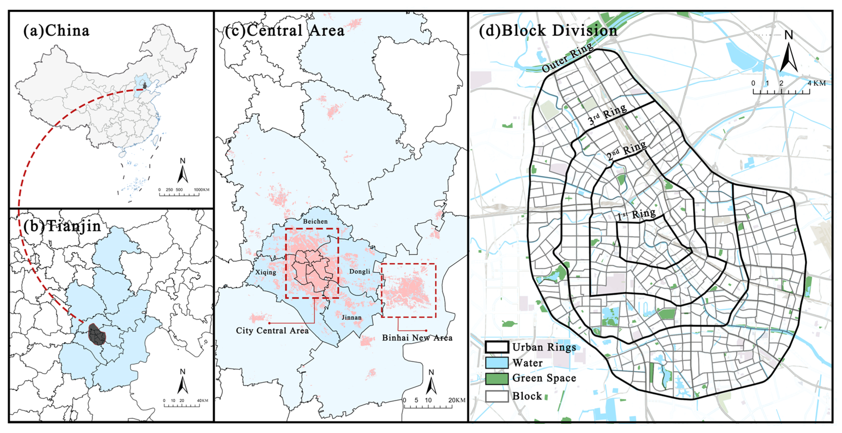
2.1. Study Area

Tianjin, one of China’s four municipalities directly under the Central Government, is a major industrial and port city in northern China. Located in the northeastern part of the North China Plain, it serves as the core city of the Bohai Economic Rim and plays a crucial role in regional economic development. By the end of 2024, Tianjin’s permanent population reached 13.64 million, with an urbanization rate of 86.01%. The study area focuses on Tianjin’s central urban area, covering 330 square kilometers. It primarily includes 11 administrative districts: Hexi, Heping, Hedong, Hebei, Nankai, and Hongqiao, along with parts of the districts of Dongli, Jinnan, Xiqing, and Beichen. As Tianjin’s core area, the central urban area is characterized by high population density, comprehensive functionality, excellent transportation connectivity, and significant variations in UV and exhibits a typical urban spatial structure defined by high density, strong functionality, and complex interactions. However, with the acceleration of urban renewal, the existing infrastructure and environment struggle to meet the growing demand for better living conditions. The region faces considerable challenges, including high living costs and competitive pressures. Furthermore, disparities in UV and BE quality are becoming increasingly pronounced. Therefore, studying UV in Tianjin’s central urban area is crucial for enhancing sustainable urban development.
Due to the precision limitations of Baidu heatmap data, differences at the street scale are not obvious because of the large area of each unit. At the community scale (with an average unit area of approximately 0.2 km2) and for smaller grid units (250 m × 250 m), the data lacks sufficient support. Additionally, the grid units tend to divide zones with the same functions into separate sections. Blocks are fundamental urban units that host the majority of socioeconomic activities. Studying UV at the block scale ensures the functional integrity of the research unit while avoiding issues caused by excessively large or small scales. Exploring the vitality patterns of blocks within a city and identifying their influencing factors is a critical approach to understanding UV [50,51]. Therefore, this study defines the research units at the block scale based on the OSM road network and remote sensing images. The average unit area is 0.74 km2, resulting in a total of 453 blocks, as shown in Figure 1.

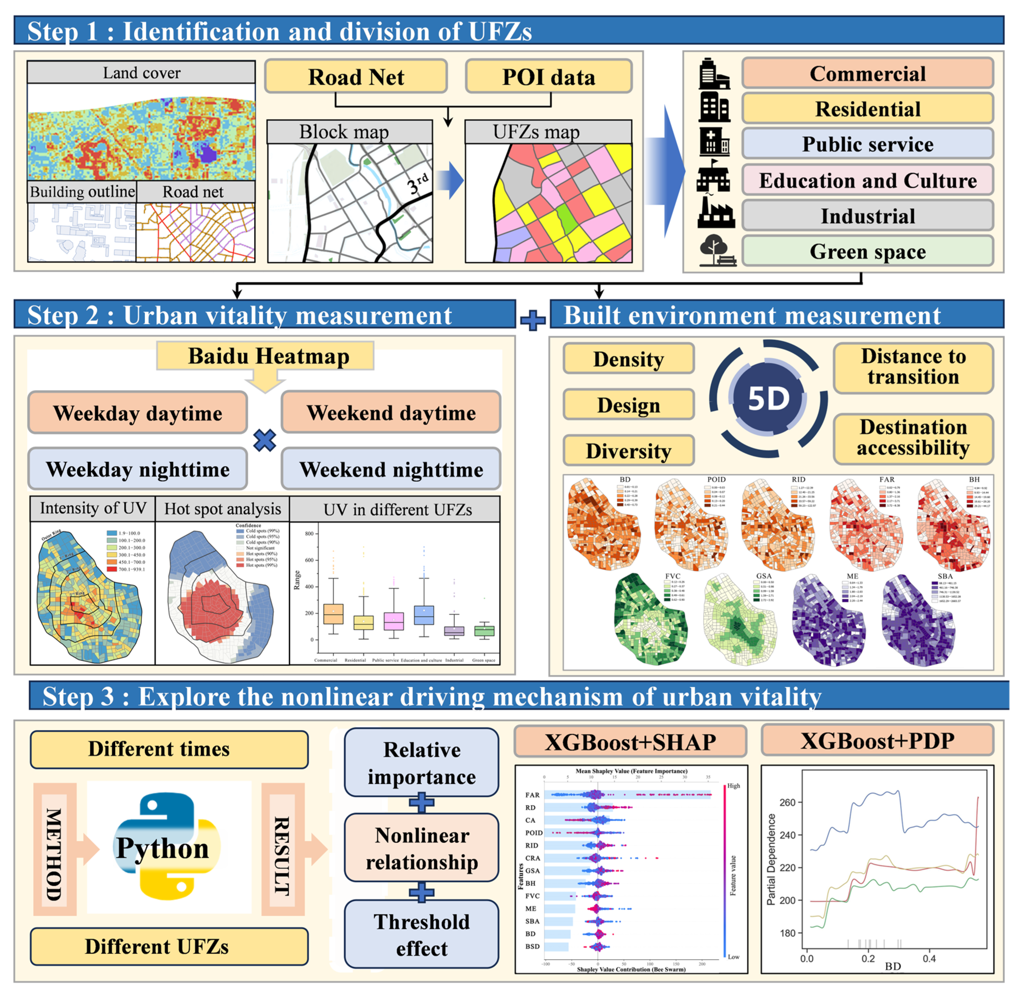
2.2. Research Framework

The proposed method is illustrated in the framework shown in Figure 2. In this study, we adopt blocks as the basic unit of analysis to explore how BE factors in different UFZs influence UV during the daytime and nighttime on weekdays and weekends. Different types of POI data are cleaned, reclassified, and used to categorize each block into a specific UFZ type. Next, UV is characterized using Baidu heatmap data and segmented into four time periods. Subsequently, BE indicators based on the 5D dimensions (such as building density, building height, accessibility, etc.) are extracted for each block for analysis. Finally, machine learning methods are employed to investigate the relationships between the BE and UV across different time periods and UFZs.

2.3. Data Source and Processing

2.3.1. Data

The basic research data used in this study include Baidu heatmap data, POI data, road network data, building data, and land cover data, as shown in Table 1. Specifically, (1) the Baidu heatmap data are obtained from the Baidu Huiyan Open Platform and capture the dynamic temporal continuity of UV. (2) The POI data and building data are sourced from the Amap Open Platform. Redundant, duplicate, and incomplete POI points are removed, and the remaining data are reclassified. They support UFZ identification and the calculation of metrics like functional density, functional mix, and accessibility. The building data are utilized to derive indicators including the building density, building height, and floor area ratio. (3) The road network data are collected from the official OSM platform. The original network was generalized to single-line representation, manually corrected against reference imagery, and topologically adjusted to facilitate block-level unit delineation. (4) The land cover data are obtained from the Geospatial Data Cloud, based on publicly available Landsat 8 imagery with a spatial resolution of 30 m. After raster processing, the data are used to calculate greening rates.

2.3.2. Urban Vitality

The flow of people in urban areas directly determines the prosperity of the region. The distribution and movement patterns of the population are the key driving forces of UV [52]. The principle of Baidu heatmap data is that when users are stationary or walking slowly, they actively visit or passively generate “location service” data, which has GPS positioning and timestamps. By providing detailed population density and activity information, it can display high-density population aggregation areas and real-time population movement. This data can accurately reflect the population distribution characteristics within smaller spatial units in the city, further expanding the application channels of big data in urban planning. Therefore, it is feasible to use Baidu heatmap data to represent the level of UV. Additionally, traditional demographic data only reflect static characteristics, while LBS mobile signaling data can capture dynamic features but are difficult to obtain and come with high processing costs [22]. In comparison, Baidu heatmap data, which are updated every 15 min, offer the advantages of easy accessibility and real-time dynamic updates, making them well-suited to revealing the spatiotemporal dynamics of human activities in urban areas. Therefore, this study employs Baidu heatmap data to characterize UV.

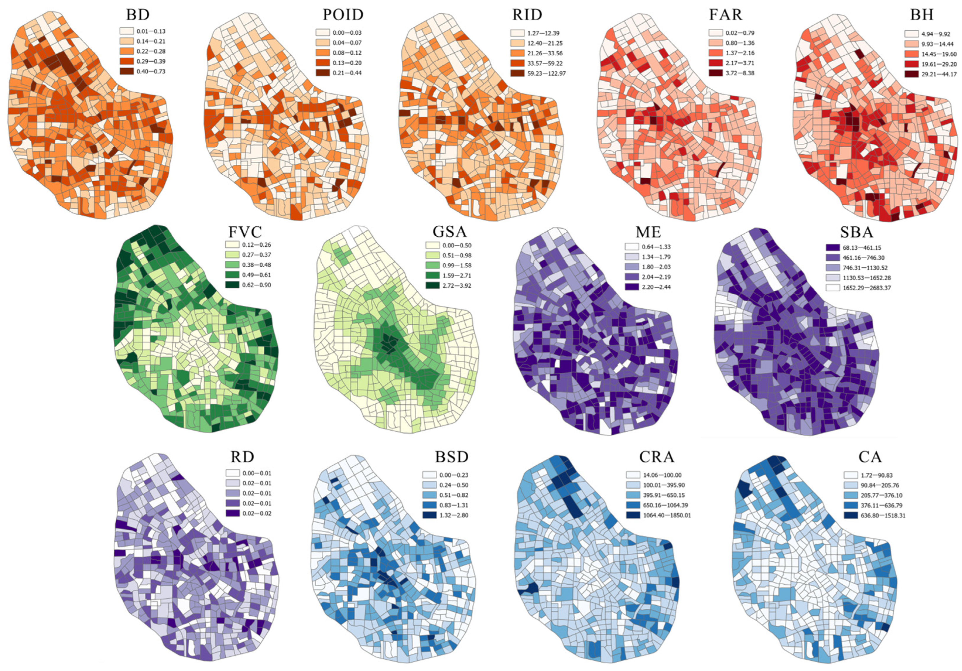
2.3.3. Built Environment

The BE refers to the various buildings and spaces created through human construction and modification [53]. This study is based on the existing BE indicator system, referencing the “5D” dimension indicator system proposed by Ewing et al. It measures the BE level in Tianjin’s central urban area from five dimensions: density, diversity, design, distance to transition, and destination accessibility. To eliminate the influence of multicollinearity among the factors, variance inflation factor (VIF) tests were conducted for each factor, and 13 BE indicators with a VIF ≤ 7.5 were retained for further analysis, as shown in Table 2.
The density dimension includes the BD, POID, and FAR, which reflect the distribution characteristics of urban space in terms of buildings and functions. The design dimension includes the RID, BH, and FVC, mainly reflecting the level and quality of the urban environment. The diversity dimension is measured by the functional mix of POIs (ME), which indicates the degree of functional diversity in the city. The distance to transition dimension includes the RD, SBA, and BSD, describing the transport convenience for urban residents. The destination accessibility dimension includes GSA, CA, and CRA, primarily reflecting the convenience with which urban residents can access various facilities for daily use. All data are projected, clipped, and unified into the divided block units for spatial data computation and analysis. Figure 3 shows the levels of various BE factors within the blocks.

2.4. Methods

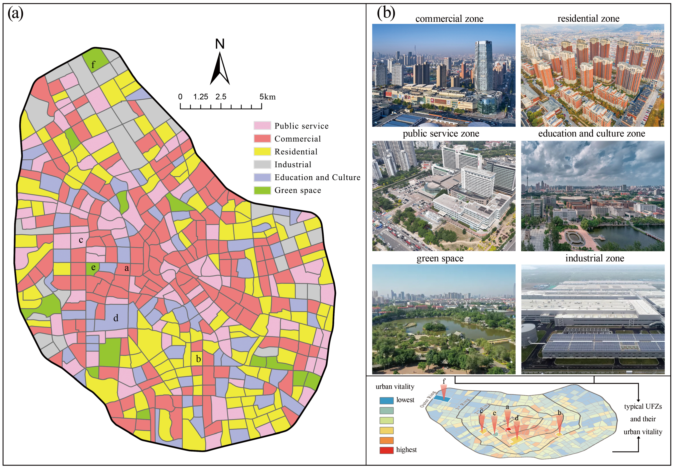
2.4.1. Identification of UFZs

In recent years, with the development of big data, many scholars have conducted research on UFZ identification using POI data combined with bus card swiping data, taxi trajectory data, etc. [54]. Open-source POI data are characterized by easy accessibility, low cost, and dynamic updates, and they can reflect information about human activities and help us to understand dynamic environments [55]. Therefore, this study uses POI data for UFZ classification. For UFZ identification, we use the frequency density and type ratio of POIs (POI feature vector) within the study unit to define the urban functional layout. The frequency density and ratio index of each block are calculated based on six types of points of interest [56]. Additionally, to facilitate comparison across different POI types, the CR vector is used to represent the percentage of each POI type within the unit based on its density. The formulas are as follows:
F i = n i N i
C i = F i i = 1 6 F i × 100 %
In the formulas, F i represents the frequency density of the i th type of POI in the research unit; n is the number of the i th type of POI in the research unit; N i is the total number of the i th type of POI in the study area; and C i denotes the proportion of the frequency density of the i th POI in the research unit. Researchers typically use a threshold of 50%, and if the CR vector value is greater than or equal to 50%, the unit is defined as a single UFZ [57]. Additionally, this study combines Baidu image data, urban land use classification data, and relevant empirical knowledge to improve the accuracy of UFZ classification. The UFZ classification results were validated and corrected through visual interpretation and manual adjustment. The classification results are shown in Figure 4.

2.4.2. XGBoost Model and SHAP Method

This study employs the Extreme Gradient Boosting (XGBoost) model to statistically analyze the impact of BE factors on UV across different time periods and UFZs. XGBoost is an enhanced version of the GBDT model that incorporates regularization terms to reduce model complexity, prevent overfitting, and improve robustness. It also handles missing values directly and is less affected by outliers [58,59]. Furthermore, XGBoost optimizes the loss function using a second-order Taylor expansion, effectively minimizing prediction errors [60]. Known for its strong performance with large-scale datasets, XGBoost is particularly well-suited for modeling complex nonlinear relationships, making it ideal for simulating the intricate relationship between the BE and UV. For XGBoost, key parameters like n_estimators, learning_rate, and max_depth are crucial for model performance. To balance the runtime and predictive performance, this paper selects 100 decision trees. The test results show that with n_estimators = 100, learning_rate = 0.1, and max_depth = 4, XGBoost achieves its highest R2, indicating better model performance.
For complex machine learning models like XGBoost, although they generally outperform traditional linear regression models in terms of accuracy and generalization, their “black-box” nature makes it difficult to interpret their internal mechanisms. To address this limitation, this study uses the SHAP method to interpret the complex impact of BE factors on UV [61]. SHAP is a game-theoretic approach that explains the marginal contribution of each feature to the model’s prediction by calculating its SHAP value, thereby reflecting the feature’s influence on the target variable [62,63]. In the UV prediction model, SHAP can identify the marginal contributions of various BE factors, enhancing the model’s interpretability and helping us understand the specific impact of BE factors on UV across different UFZs and time periods.

3. Results

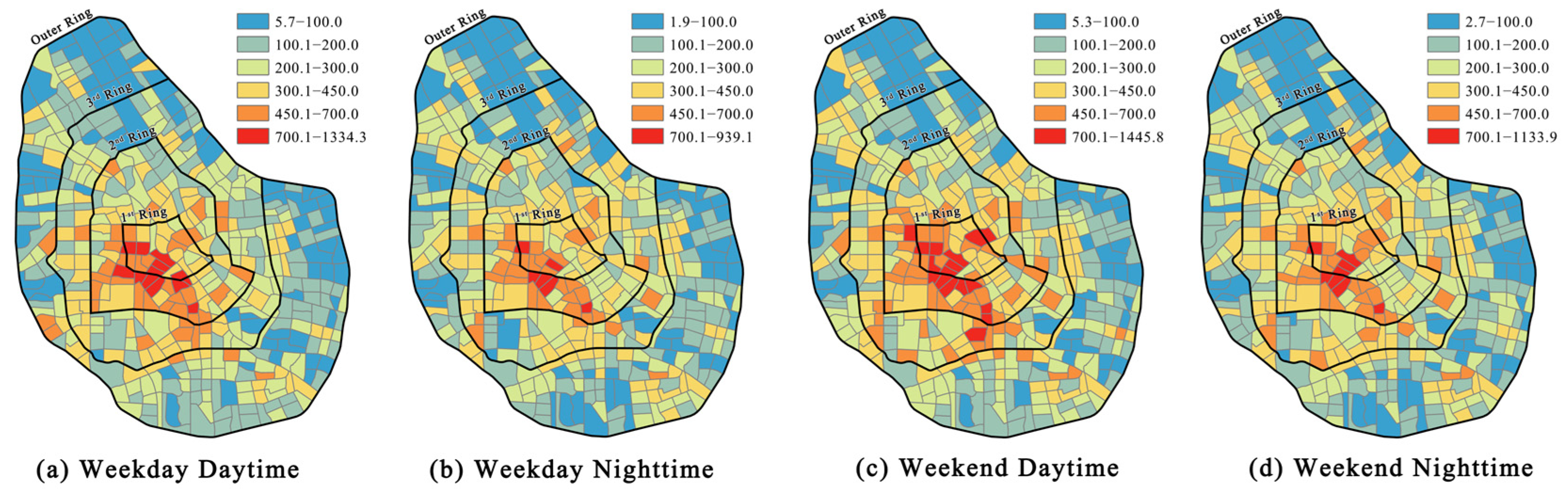
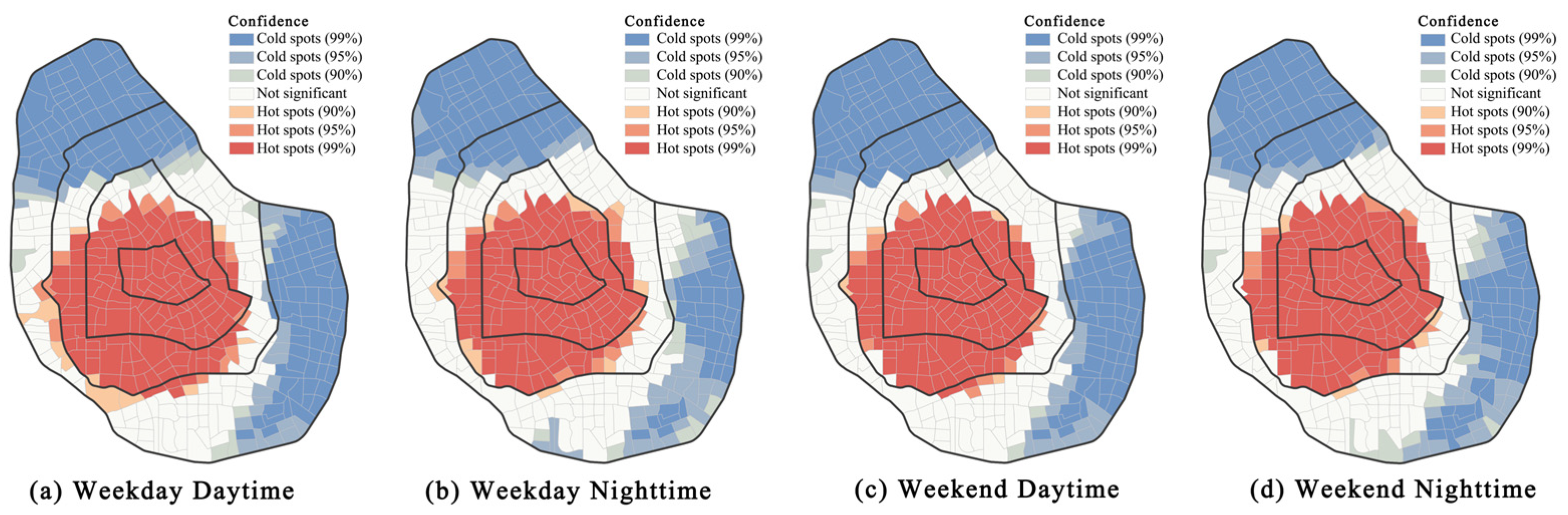
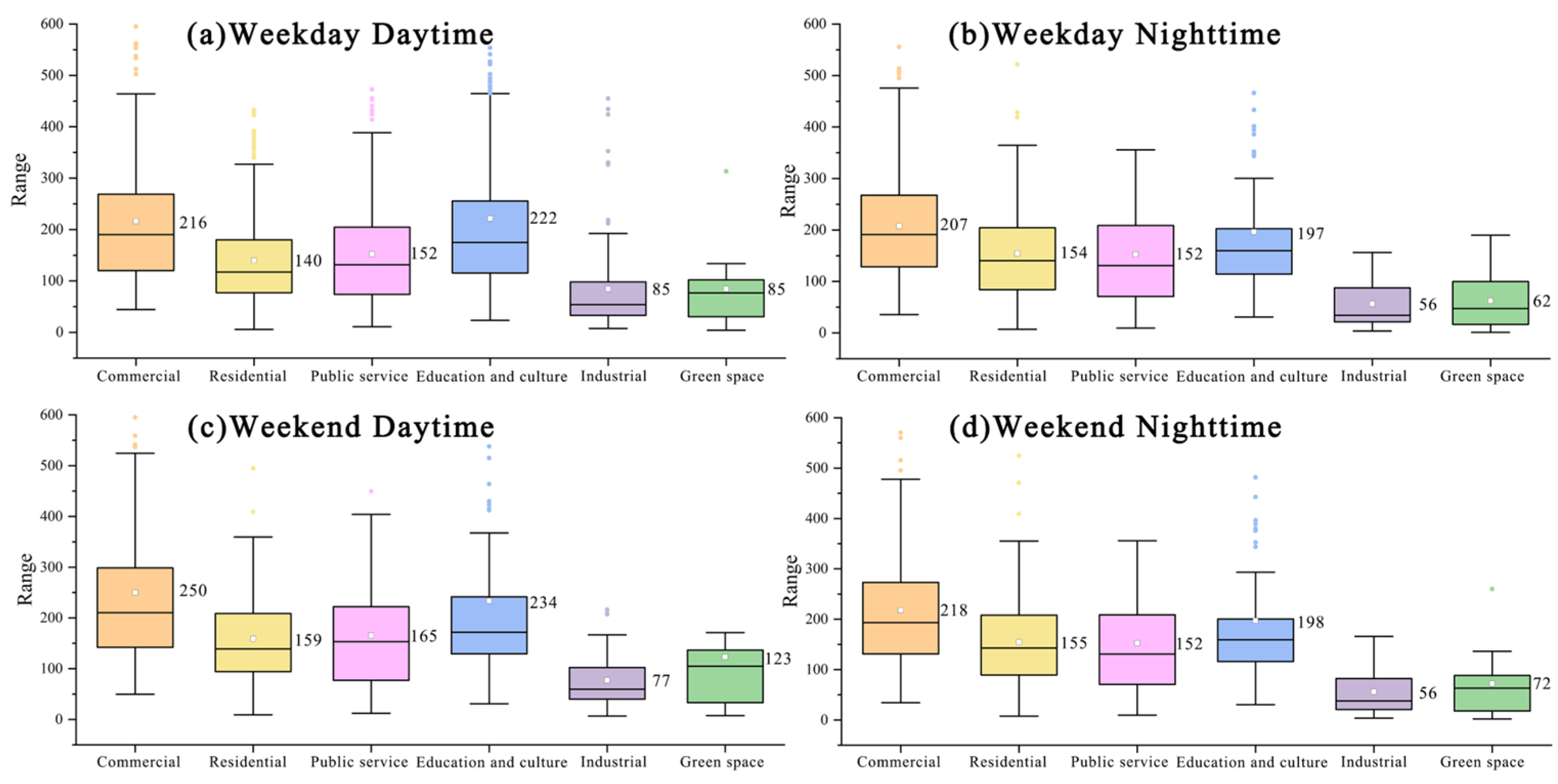
3.1. Spatial Distribution of Urban Vitality Across Different Times

Table 3 presents the differences in UV across different time periods. Comparing the four time periods reveals that UV is highest and most volatile during the daytime on weekends, with an average value of 194.8, while it is lowest and least volatile during the nighttime on weekdays, with an average of 166.9. During weekend nights, although UV decreases to an average of 172.7, it remains relatively close to the daytime UV on weekdays, which has an average value of 174.8. Overall, UV shows significant temporal variation, with higher UV typically observed during the daytime compared to the night and higher UV on weekends compared to on weekdays. These differences highlight the rhythmic nature of human activity and reflect the strong connection between activity patterns and time.
Using the natural breaks method, the UV values in Tianjin’s central area were classified, revealing how UV varies across different times, as shown in Figure 5. In all four time periods, the pattern of UV shows higher values in the center and lower values on the periphery, with a clear radial structure. Specifically, the core areas exhibit higher UV concentrations, which gradually decrease towards the outer regions, indicating a declining trend from the center outward. Zones with high UV are mainly located in the heart of the central city, which features abundant commercial and tourism resources, as well as well-developed infrastructure, making it a hub for high-density human activity. Zones with low UV are primarily found in the northern and eastern parts, where the zones are mainly residential and industrial. Hot spot and cold spot analysis further emphasizes the “single-center” vitality distribution in the city, Figure 6. Compared to in the daytime, UV at the edges of the central area increases at night, while UV in the core area decreases. On the one hand, the central area is bustling with workers during the daytime, but at night, residents from the outskirts return home, which boosts UV in those areas. On the other hand, the use of Baidu-related mobile apps may decrease at night, leading to a drop in activity in the center.
Figure 7 illustrates the spatial distribution of urban vitality across different UFZs during four time periods. Overall, commercial zones and education and culture zones consistently exhibit higher levels of UV compared to other functional zones, while industrial zones and green space remain at relatively low levels. UV is generally higher during the daytime than at night across all UFZs. However, residential zones show a contrasting pattern on weekdays, with lower UV during the daytime (140) than at night (154). Across different UFZs, UV tends to be higher on weekends than on weekdays, except for in industrial zones, which demonstrate greater UV during weekdays. Apart from industrial zones, UV in other UFZs reaches its peak during the daytime on weekends, reflecting a significant increase in residents’ activities in commercial, cultural, and recreational spaces during this period. During weekday daytime, education and culture zones record the highest UV levels, whereas in other time periods, commercial zones dominate, with UV peaking during weekend daytime (250) and dropping to a lower level during weekday nights (207). The UV of education and culture zones is comparable to that of commercial zones, particularly prominent during weekday daytime (222) and weekend daytime (234), but declines at night. Public service zones exhibit moderate and relatively stable vitality, with minor fluctuations across time periods. In residential zones, UV peaks during weekend daytime (159) but drops to its lowest point during weekday daytime (140), while nighttime UV remains relatively high, reflecting the typical temporal usage patterns of residential zones. Compared to other time periods, green space shows a notable increase in UV during weekend daytime (123). Industrial zones reach their highest UV during weekday daytime. However, compared to other UFZs, industrial zones consistently exhibit the lowest UV across all time periods.

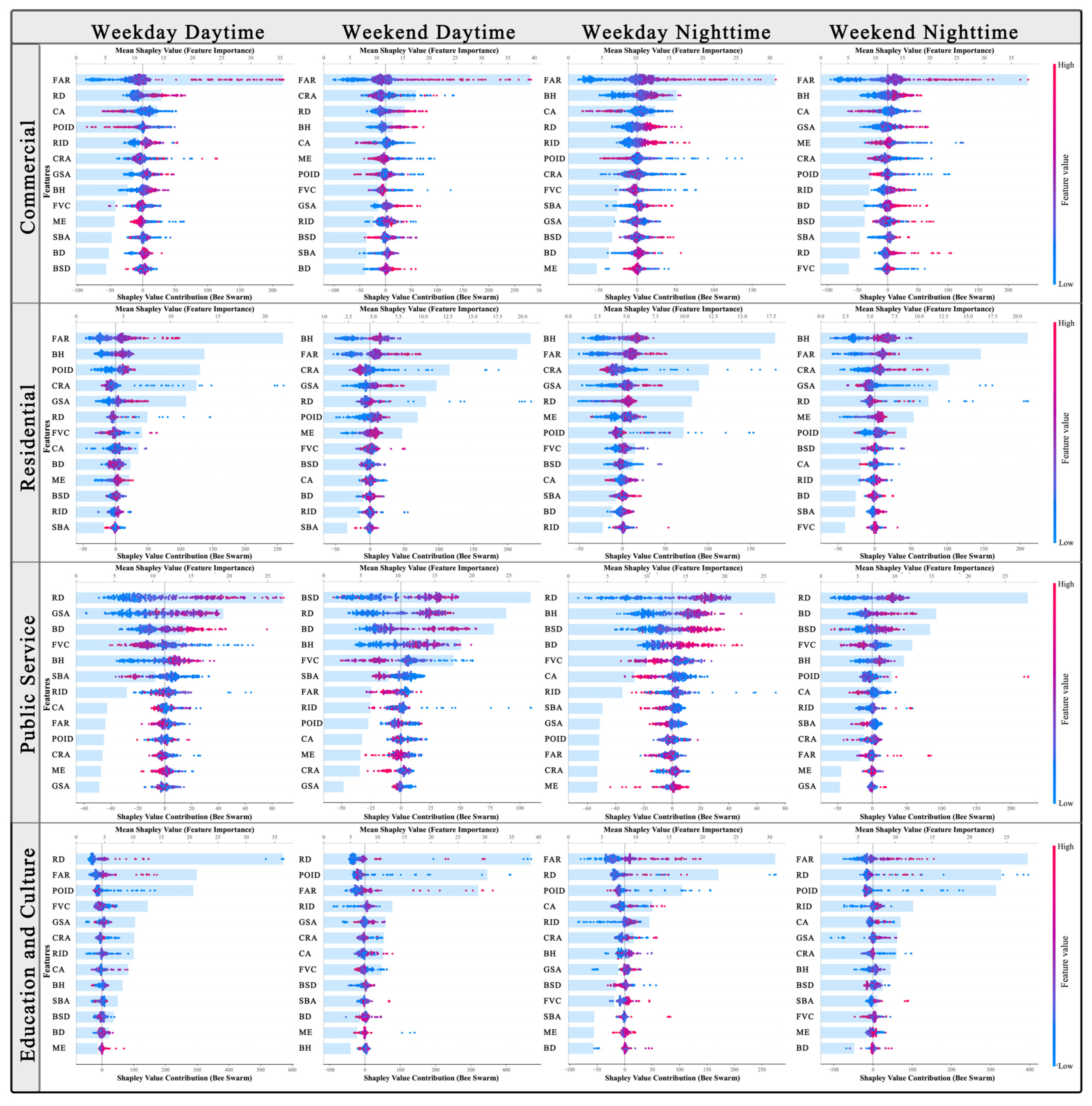
3.2. Relative Impact of Built Environment on Urban Vitality Across Different Times and UFZs

To analyze the impact of BE factors on UV across different times and UFZs, we selected four types of urban functional zones with higher UV values for study. Using the XGBoost model, we calculated the relative contribution of each indicator and visualized their SHAP values. This allowed us to assess the contribution and impact trends of various BE characteristics across different time periods and UFZs. The BE features were ranked in descending order based on their overall contribution to UV. A higher contribution indicates a greater influence of the BE on UV. The bee swarm plot demonstrates the overall impact trend of BE characteristics on UV, with values to the left of zero representing a negative impact and values to the right indicating a positive impact. The results are shown in Figure 8.
The contribution of the BE to UV is closely related to different times and UFZs. Overall, the impact of the BE on UV varies significantly across different UFZs, while the contribution within the same urban functional zone remains relatively consistent across time periods. Specifically, in commercial zones, the FAR has the most significant impact, while RD and BSD play a larger role in the public service zone. In education and culture zones, RD, POID, and the FAR exert a stronger impact on UV. In residential zones, UV is not only influenced by the FAR but also closely associated with BH, GSA, and CRA, reflecting the behavioral patterns and needs of residents.
Within the density dimension, the FAR strongly enhances UV in commercial, residential, and education and culture zones across all four time periods. In contrast, it exerts a relatively minor influence on public service zones, where an increased FAR even suppresses UV. POID significantly affects UV in education and culture zones. However, increased POID only promotes UV in residential zones. In other urban functional zones, it consistently shows a suppressive effect on UV. BD exerts a particularly strong impact on UV in public service zones, significantly enhancing UV as BD increases.
Within the design dimension, BH has a substantial impact on UV in commercial, residential, and public service zones, with the strongest influence observed in residential zones during weekday nights and weekends. FVC plays a particularly significant role in public service zones, where higher levels of vegetation coverage tend to suppress UV. In other urban functional zones, FVC shows different levels of impact on UV and only slightly improves UV in residential zones. RID shows a relatively low contribution in residential zones but demonstrates a strong positive effect on UV in commercial zones.
Within the diversity dimension, the ME contributes to UV in both commercial and residential zones. In commercial zones, the impact of the ME on UV is stronger during weekends and tends to be suppressive. In residential zones, the influence is stronger at night than during the day and shows a positive effect. This indicates that residential zones rely more on a diverse functional mix to meet the residents’ daily needs compared to commercial zones.
The distance to transition dimension shows the highest overall contribution to UV in public service zones. RD has a strong positive impact on enhancing UV in open spaces such as commercial, public service, and education and culture zones. However, RD tends to suppress UV in residential zones, which are more private spaces. In commercial zones, the SBA has a stronger influence on UV during weekends compared to BSD. In other urban functional zones, BSD contributes more to improving UV than the SBA. This effect is particularly obvious in public service zones, where higher BSD and a better SBA are both favorable for promoting UV.
Within the destination accessibility dimension, GSA makes a significant contribution to UV in commercial, residential, and education and culture zones. In particular, improving GSA notably enhances UV in residential zones. CA strongly promotes UV in commercial zones, while it shows a negative contribution in education and culture zones. In public service zones, CA has a positive effect on UV, with a greater impact observed at night than during the day. CRA greatly promotes UV in residential zones and contributes most to UV in commercial zones during the daytime on weekends.

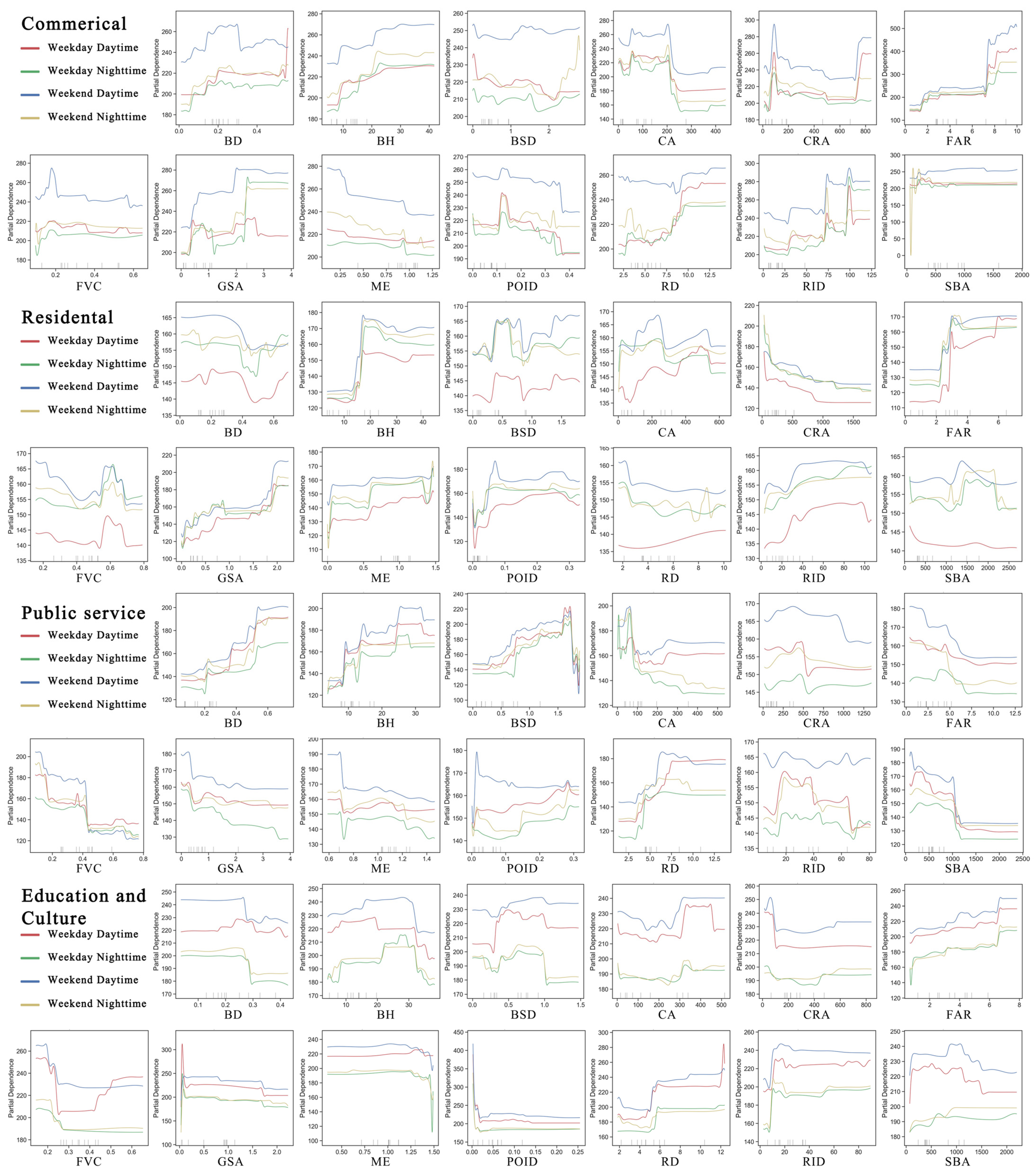
3.3. Nonlinear Relationship and Threshold Effect Between Built Environment and Urban Vitality Across Different Times and UFZs

To explore the relationships between BE indicators and UV across different UFZs and time periods, we plotted partial dependence plots (PDPs) to illustrate the impact trends of each feature on UV, highlighting the nonlinear relationships and threshold effects across UFZs, as shown in Figure 9. Overall, the influence trends of each indicator on UV remain relatively consistent across different time periods but show substantial variation across different UFZs.
In commercial zones, within the density dimension, BD generally exhibits an initial positive effect on UV, which then levels off beyond a threshold of 0.2. However, during the daytime on weekends, BD begins to show a negative impact once it exceeds 0.3. The FAR displays a clear threshold effect: UV increases sharply as the FAR rises from 1.2 to 2.0, then stabilizes with diminishing marginal benefits between 2.0 and 7.2. When the FAR exceeds 7.2, UV rises steeply again, likely reflecting the high levels of UV associated with highly developed commercial centers. POID shows a generally negative relationship with UV, with a brief increase reaching a peak around 0.14, followed by a downward trend up to 0.35. Within the design dimension, BH positively contributes to UV when below 24 m, after which its effect tends to level off. RID shows greater variability: UV increases gradually at lower densities, but two distinct peaks are observed when RID reaches approximately 75 and 100. In the diversity dimension, the ME exhibits a strong negative correlation with UV, particularly during the daytime on weekends, where UV significantly declines once the ME exceeds 0.25. Within the distance to transition dimension, RD has a stronger positive effect on UV during weekend nights and weekdays, especially in the 7.5 to 9 range, whereas its impact is weaker during weekend days. The SBA shows a strong positive effect when the distance is short (<200 m), but the effect stabilizes once this threshold is exceeded. In the destination accessibility dimension, GSA has a weak effect during weekday daytime but shows significant positive effects when reaching thresholds of 0.6 and 2.3 during other periods. CA shows a decreasing trend, with a pronounced negative impact when accessibility drops (>200). CRA shows an overall declining trend, peaking when accessibility reaches around 100. Finally, FVC and BSD exhibit relatively weak effects in commercial zones and do not display clear nonlinear relationships with UV.
In residential zones, within the density dimension, BD has a gradual effect on UV between 0 and 0.35 but shows a significant decline once it exceeds 0.35. The FAR remains stable between 0 and 2, but when it exceeds 2, UV rises sharply and stabilizes around 3. POID generally has a positive effect on UV, with a notable increase in UV between 0.05 and 0.1. However, beyond this threshold, the marginal benefit of increasing POID diminishes. In the design dimension, BH has little impact on UV between 0 and 18 m, but it increases rapidly and stabilizes at a higher level once it exceeds 18 m. RID significantly boosts UV between 20 and 35. FVC has a weak positive effect on UV when below 0.5, but when it reaches 0.6, UV improves significantly across all time periods. However, further increases in FVC tend to suppress UV. Unlike in commercial zones, the ME shows a clear positive effect on UV. In the distance to transition dimension, RD and the SBA show no significant effects during weekday daytime. RD exhibits a slight positive effect during the daytime on weekdays but has a negative impact during other time periods. UV significantly drops, especially between 2 and 3, then stabilizes. The SBA shows a downward trend during weekday daytime, but during other times, UV increases significantly between 1500 and 2000. BSD shows an up–flat–down–up trend with high volatility, generally demonstrating a positive influence. In the destination accessibility dimension, GSA shows significant positive effects, especially between 0 and 0.75, where the impact is more noticeable. As it approaches 1.5, the improvement in UV becomes more pronounced, with further increases enhancing marginal benefits. CRA reduces UV as the distance increases from 0 to 150, after which it stabilizes at a lower level. CA has high volatility, showing a decrease–increase–sharp decline pattern, with a peak at 250.
In public service zones, within the density dimension, BD shows a clear positive effect on UV, with certain differences between day and night. Two key thresholds exist: when BD exceeds 0.35 and 0.5 during the day, and 0.2 and 0.5 at night, UV significantly increases. The FAR generally demonstrates a negative impact on UV, with UV remaining at higher levels in the lower range (0–4.5) across all time periods but significantly decreasing beyond this range. POID exhibits a weak positive trend. In the design dimension, BH generally has a positive effect, with significant increases in UV when it exceeds the thresholds of 8 and 24 m. RID shows a weak effect during weekday daytime, but its impact increases initially and then decreases during other time periods. The influence is most pronounced between 0 and 35. However, once it exceeds this range, it starts to suppress UV. The ME generally shows a negative correlation with UV. In the distance to transition dimension, RD and BSD both positively influence UV. RD shows a higher marginal benefit at night, with UV increasing until it exceeds 5, after which the effect gradually diminishes. During the day, this threshold rises to 7. As BSD increases, UV rises significantly, peaking at around 1.5, after which it rapidly declines. The SBA has a stronger impact at lower values, but UV sharply decreases when the distance exceeds 1000 m. In the destination accessibility dimension, GSA has a higher positive effect on UV at lower values, but this declines as GSA increases, with a noticeable drop during weekend nights. CA positively impacts UV within the range of 0–70. However, once this threshold is exceeded, it becomes negative with UV decreasing rapidly. CRA boosts UV within the range of 0–500, but UV declines and stabilizes once the threshold is surpassed.
In education and culture zones, within the density dimension, BD generally shows a negative impact on UV, with minimal influence during weekday daytime. However, during other time periods, UV decreases significantly once BD exceeds a threshold of 0.27. The FAR and POID consistently improve UV, but the improvements are not strong. In the design dimension, BH has a positive effect on UV when below 30 m, but UV rapidly decreases once it exceeds 30 m. RID shows a positive effect in the range of 8–15, with higher marginal benefits, but beyond 15, further increases in RID have only a minimal impact on UV. FVC shows a “U”-shaped impact on UV during weekday daytime. The ME has no significant effect in the range of 0–1.2, but once it exceeds 1.25, it shows a clear negative effect on UV. In the distance to transition dimension, RD demonstrates a strong positive effect on UV, with UV increasing sharply when RD reaches 5. Beyond this threshold, further increases in RD contribute weakly to UV. BSD positively influences UV in the range of 0–1, but this begins to decline after it exceeds 1, with a more significant effect at night. The SBA maintains a high level during the day within the range of 0–1000 m, after which UV gradually declines. At night, the SBA shows a weak positive impact. In the destination accessibility dimension, GSA has a relatively low negative effect on UV. CA generally shows a negative trend, with UV decreasing as the distance to commercial facilities decreases. CRA shows high UV within a low range (0–100), but UV rapidly decreases after exceeding 100, with a particularly notable decline during the daytime.

4. Discussion

4.1. Influence of Built Environment on Urban Vitality Across Times and UFZs

It is widely proven that the BE significantly influences UV. Many studies show that different dimensions of the BE, such as density, accessibility, and diversity, have a significant impact on UV [64,65]. Based on UFZs, this study found that the impact of the BE on UV varies significantly across different UFZs, which is due to the differing functions and demands of the populations served by each function zone. This study found that the FAR makes a significant contribution to all urban function zones except for public service zones, indicating that a higher FAR is more likely to stimulate UV in areas primarily focused on commercial, residential, educational, and cultural functions. However, excessive development may lead to spatial congestion, affecting the use of public spaces. BD shows a particularly significant effect in public service zones, while BH has a notably strong impact in residential areas but is not significant in other function zones. This suggests that increasing BD or BH may not necessarily enhance UV in certain function zones, which is consistent with the findings of Chen et al. [21]. Additionally, higher FVC tends to suppress the enhancement in UV in public spaces, indicating that excessive green coverage may limit the space for public activities and social interactions, aligning with the research of Mou et al. [66]. Jane Jacobs proposed that smaller block patterns are more likely to promote human activity within a neighborhood. However, Gan et al. found that this pattern does not significantly enhance UV if conditions such as safety and a pedestrian-friendly environment are not met [67]. In this study, RD exhibits a suppressive effect on UV in residential zones, which are more private spaces. We found that higher RD does not improve UV in residential zones, which is inconsistent with some studies [23,68]. However, it can promote UV in commercial, public service, and education and culture zones, which are more open spaces. This could be due to better connectivity, making it easier for residents to access service facilities and public spaces [69]. Therefore, residential zones require good pedestrian environments, while open spaces need efficient transportation networks to enhance UV. Some existing studies show that proximity to transit and transportation facilities significantly affects UV, with subway stations playing an important role in enhancing UV [29]. However, in our study, we found that BSD and the SBA have a larger contribution to UV in public service and commercial zones, particularly in public service zones. In contrast, they do not have a significant impact on UV in other zones. This may be due to the fact that transport station usage tends to follow peak-time patterns. An increase in the ME and POID makes a positive contribution to UV in residential zones, indicating that residential zones require more intensive and diverse functions to meet residents’ living needs. This finding is consistent with earlier studies [3,70]. However, in commercial zones, these factors exert a suppressive effect, as overly complex functional layouts may lead to spatial conflicts, inhibiting the enhancement in UV in commercial zones. Destination accessibility has varying impacts on UV across different UFZs. This study found that better CA increases UV in commercial zones but suppresses it in education and culture zones. The presence of more commercial facilities, such as shopping and dining, may negatively affect the UV of zones primarily focused on scientific and educational functions. This differs from existing studies [7,21]. GSA and CRA positively impact UV in residential zones, indicating that residents rely on parks, green spaces, and cultural or recreational facilities for social and leisure activities. However, in public service zones, the closer the green space, the lower the UV, which aligns with the findings of Lixin et al. [36].

4.2. Threshold Effects of Built Environment on Urban Vitality Across Times and UFZs

Numerous studies have demonstrated nonlinear characteristics and threshold effects in the correlation between the BE and UV [71,72]. This study reveals the differences in how various BE factors influence UV across different time periods and UFZs. The findings are similar to those of some existing studies but also present certain differences.
In commercial zones, the FAR shows a significant positive impact on UV, which aligns with previous studies [73]. In our study, it exhibits two clear thresholds, possibly reflecting two types of commercial spaces: For street-level shops or small commercial blocks, UV tends to plateau when the FAR reaches 2. This usually corresponds to low-rise buildings of two to four floors, which is a very common ground-floor commercial form. It can form continuous street interfaces (such as shop signs and display windows), maximize the accessibility of pedestrians’ lines of sight, and increase the probability of random consumption. For larger commercial areas, typically accompanied by high-rise buildings such as business hotels and offices, UV increases dramatically when the FAR reaches 7.2, after which it stabilizes at night but continues to rise during the day, especially on weekends. Commercial centers have a small footprint and usually require a higher floor area ratio to meet the activity needs of abundant people. This characteristic is also evident in BH, where two thresholds of 10 and 20 exist, though the trend is less pronounced compared to the FAR. In residential zones, both BH and the FAR exhibit a sharp increase followed by stabilization when reaching thresholds of 18 and 3, respectively, which are higher than those in commercial zones. Although higher density can accommodate more residents, a further increase in the residential population does not seem to significantly promote UV [43]. However, the FAR suppresses UV in public service zones, as excessive development and diversity can lead to the overcrowding of residents and their activities, which in turn increases psychological stress, thus hindering UV [23]. The impact of BH in these two zones is the opposite, with increased vertical space not enhancing the UV of education and culture zones. Chen et al.’s research found that in high-density urban zones, BD does not directly reflect UV [20]. Our study found that BD promotes UV in commercial and public service zones but has a suppressive effect in residential and education and culture zones. In commercial zones, BD’s effect on UV levels off after reaching a threshold of 0.2. On weekends, this threshold increases, and UV begins to decline after BD reaches 0.3, likely due to crowded conditions in commercial zones during the daytime on weekends, where excessive BD may lead to congestion, affecting the overall UV. BD has a significant positive impact on UV in public service zones, with noticeable day–night differences, possibly due to the lower usage of public facilities at night. In residential zones, BD’s influence on UV follows a trend of decline followed by an increase. UV starts to decline after BD exceeds 0.35 but increases again after surpassing the inflection point of 0.45. This trend is particularly noticeable on weekdays. In education and culture zones, BD exhibits a clear threshold effect, with a significant decline in UV after it exceeds 0.25. This reflects that high density may cause a sense of spatial pressure and traffic congestion, which in turn discourages residents from going out. Therefore, building regulations should maintain a reasonable range to avoid these negative effects.
Early studies suggest that functional diversity is a major source of UV [1,6]. Many existing studies indicate that diverse functions positively contribute to UV [74,75]. However, in our study, this positive effect is only observed in residential zones. A community without the appropriate quantity and variety of facilities cannot attract people or sustain social interactions. Once the POID exceeds 0.1 and the ME exceeds 0.6, the marginal benefit of their increase on UV becomes weak. Research by Kosta et al. suggests that an excess of commercial facilities may disrupt social interactions within residential zones [66]. In contrast to residential zones, the POID and ME show a negative impact on UV in commercial zones. The POID peaks at 0.14, then declines rapidly, but this change is less pronounced during weekend daytime. It drops again sharply after reaching 0.35. The ME shows greater variation during weekend daytime, with less fluctuation at other times. This may be due to overly dense or mixed facilities, which can complicate commercial spaces, diluting consumers’ decision-making paths and reducing their willingness to stay [76]. In public service zones, the ME has a suppressive effect, with UV rapidly declining after it exceeds 0.7, especially during weekend daytime. In education and culture zones, the impact of the ME is minimal, possibly because the land use feature for schools and cultural facilities does not require overly complex functions.
In commercial zones, RD and RID significantly contribute to enhancing UV. RD leads to a substantial increase in UV when it reaches 7.5, stabilizing after 9. Its impact is less pronounced during weekend daytime. At low densities, the effect of RID on UV remains relatively stable, but when RID reaches 75, UV increases sharply. This indicates that commercial zones require high levels of street network complexity and connectivity to foster UV. RID also has a positive impact on UV in residential zones, which contrasts with the findings of Chen et al.’s study in a residential zone in Shenzhen [21]. RD shows temporal differences in residential zones. During weekday daytime, RD has a modest positive effect on UV, while it suppresses UV during other times. This differs from the effect in commercial zones, likely due to the negative impacts of high RD, such as traffic congestion and noise pollution, which degrade the quality of the residential environment and inhibit UV improvement. This temporal difference suggests that the movement and activities of residents are influenced by the relationship between work and residence, which is why RD’s effect differs during weekdays. RD and RID both show positive effects in education and culture zones. In public service zones, RD significantly enhances UV, with higher saturation levels during the day compared to at night, indicating that higher RD is more critical during the day for boosting UV. However, RID shows high UV at lower values (0–20), with a significant decline after exceeding 40, but the effect is minimal during weekend daytime. The SBA and BSD show no significant impact in commercial zones, likely due to the high density and coverage of public transport facilities in these zones. In residential zones, the SBA peaks at longer distances (1500–2000 m), and BSD shows a peak in the lower range (0.4–0.9). In education and culture zones, both the SBA and BSD exhibit temporal differences, promoting UV during the daytime and having the opposite effect at night. Moreover, BSD shows a threshold effect, with UV declining once it exceeds 1. The SBA and BSD significantly promote UV, but once the distance from subway stations exceeds 1000 m, UV sharply decreases. This suggests that subway stations should maintain a service radius within 1 km.
FVC exhibits various negative impacts on UV across different UFZs. Li et al.’s research also identified this negative effect, though their study found that UV decreased in communities closer to parks [35], which differs from our findings. In residential zones, FVC reaches a peak at 0.6 and has a minimal impact on commercial zones. In public service zones, FVC has a significant suppressive effect, with UV rapidly declining once it reaches 0.4. In education and culture zones, this threshold is even lower (0.2). Unlike other time periods, FVC shows a positive effect on UV after it exceeds 0.4 during weekday daytime, likely due to the fact that certain facilities, such as schools, science museums, and cultural centers, operate mainly during weekday daytime and are well-integrated with green spaces. In the destination accessibility dimension, GSA positively influences UV in commercial and residential zones but has a suppressive effect in public service zones, with minimal impact in education and culture zones. In residential zones, the marginal benefits of GSA decrease when kernel density reaches 0.8 and then increase again when it reaches 1.8. In commercial zones, CRA causes a sharp decline in UV when it exceeds 100. Residential and education and culture zones show similar trends, but in education and culture zones, the effect at night is almost negligible. This reflects that urban residents strongly depend on leisure activities in their daily lives.

4.3. Limitations and Future Studies

This study deeply explored the impact of the BE on UV in Tianjin’s central urban area from the perspective of UFZs. It reveals the relative importance and nonlinear relationships between BE characteristics and UV across different UFZs and time periods, offering valuable insights for urban planning and function layout optimization. However, there are several limitations in this study: Firstly, given that this study is based on a case study of Tianjin’s central urban area, the conclusions drawn have not yet been verified for their applicability to other cities. Secondly, this study measures urban vitality using data from a single month, which may overlook the potential long-term dynamics of urban vitality, such as seasonal and annual variations. Thirdly, many scholars comprehensively characterize UV through integrated dimensions such as social vitality, economic vitality, and cultural vitality [5,33]. This study employs Baidu heatmap data to characterize UV, which can effectively capture the spatiotemporal dynamics of UV. However, it may neglect the impact of socioeconomic conditions and cultural richness on urban vitality [77]. Finally, existing research has found that BE features exhibit interactive effects and jointly influence UV [22,43]. Multiple variables exhibit threshold effects in their synergy, causing local impacts to switch between negative and positive [5]. This study has not analyzed potential interactive effects between these features. The situation where different BE elements may interact and jointly affect UV remains to be further studied.
Future studies may expand on this subject in the following areas: First, given that analysis confined to a single city limits generalizability, future research will incorporate multi-city and multi-scale comparative analyses to examine their divergences and similarities. Second, future research should incorporate longitudinal data to capture dynamic UV patterns across seasons and years, thereby better revealing the long-term impacts of the BE on UV. Third, future studies should conduct multidimensional assessments of urban vitality by incorporating socioeconomic and cultural data to provide a more comprehensive understanding of the underlying mechanisms driving UV formation and changes. Finally, future studies should adopt diverse machine learning models to better untangle the complex impacts of BE factors on UV, particularly their interactive relationships.

5. Conclusions

This study evaluates the UV on weekdays and weekends in Tianjin’s central urban area using Baidu heatmap data and compares the temporal differences from the perspective of UFZs. It further explores the nonlinear influence and threshold effects of BE factors on the spatiotemporal variation in UV. The main findings are as follows:
(1) UV exhibits significant temporal and spatial variation. Overall, UV is generally higher on weekends than on weekdays and higher during the daytime than at night. UV is the highest with the greatest volatility during the daytime on weekends, while UV is the lowest and most stable on weekday nights. The UV of education and culture zones is highest during weekday daytime, while in other time periods, commercial zones exhibit the highest UV. Industrial zones consistently show the lowest UV across all time periods. In residential zones, UV is higher during the nighttime than the daytime on weekdays, while the opposite is observed on weekends. In public service zones, UV remains similar between day and night on weekdays. For all other UFZs, UV during the daytime exceeds nighttime levels. On weekend days, all functional zones except for industrial zones show the highest levels of UV.
(2) In commercial zones, the FAR, BH, RD, and CA are the most influential BE factors. The FAR demonstrates a clear threshold effect: UV increases rapidly within the 1.2–2 range, flattens between 2 and 7.2, and then sharply rises again beyond 7.2. BH positively contributes to UV when below 24 m, beyond which its effect plateaus. RD more significantly boosts UV during weekday and weekend nights, especially between 7.5 and 9, while its effect is limited during weekend daytime. CA shows a decreasing trend, with a strong negative effect when accessibility exceeds a threshold of 200.
(3) In residential zones, BH, the FAR, CRA, and GSA have strong impacts on UV. BH has a minimal influence on UV below 18 m but sharply increases UV beyond this threshold and then stabilizes at a high level. The impact of the FAR on UV remains flat below 2, but UV rises rapidly once it exceeds this threshold and stabiles around 3. CRA negatively correlates with UV, with a decline observed within the 0–150 range before stabilizing. GSA exhibits a strong positive effect, particularly within the 0–0.75 range, and becomes more pronounced around 1.5, showing increasing marginal benefits.
(4) In public service zones, RD, BSD, BH, BD, and FVC exert more impacts on UV. RD shows higher marginal benefits at night, with UV gradually declining beyond 5, while this threshold increases to 7 during daytime. BSD shows a clear peak around 1.5, after which UV declines rapidly. BH generally promotes UV, with sharp increases observed after the 8 and 24 m thresholds. BD shows a strong positive influence on UV, with evident day–night differences. Specifically, two key thresholds are identified: UV increases significantly when BD exceeds 0.35 and 0.5 during daytime and 0.2 and 0.5 at night. FVC demonstrates a strong negative effect, particularly beyond the 0.4 threshold, where UV drops sharply across all time periods.
(5) In education and culture zones, RD, the FAR, and POID have a greater influence on UV. When RD reaches 5, UV increases rapidly, but its marginal effect weakens beyond this threshold. The FAR and POID consistently promote UV, though their effects are relatively moderate.
This study enables urban planners and policymakers to focus more on the spatiotemporal impacts of BE features on UV. It highlights the need for customized management strategies for different UFZs, offering refined references to enhance UV around the clock. In order to achieve the most effective enhancement in UV, each UFZ should be optimized, considering how BE features affect UV and their underlying mechanisms. This research reveals the nonlinear relationships between these BE features and UV, with specific upper and lower limits for variables such as the FAR, BD, RD, SBA, and ME, which show threshold effects. Identifying the thresholds of BE attributes provides empirical support to the development of planning guidebooks that are crucial for effective planning practice. Planners are advised to optimize the BE by referring to the value ranges of these indicators, thereby guiding the efficient allocation of spatial resources. For instance, maintaining an RD of around 10 in commercial zones can ensure that road traffic capacity optimally promotes UV. Additionally, targeted BE plans and policies should be formulated based on these insights to effectively enhance UV.

Author Contributions

Conceptualization, F.S. and E.W.; methodology, F.S.; software, F.S.; validation, F.S.; formal analysis, F.S.; investigation, F.S.; resources, F.S.; data curation, F.S.; writing—original draft preparation, F.S.; writing—review and editing, F.S. and E.W.; visualization, F.S.; supervision, E.W.; project administration, E.W.; funding acquisition, E.W. All authors have read and agreed to the published version of the manuscript.

Funding

This research was funded by the Basic Scientific Research Foundation of the Educational Department of Liaoning Province (JYTMS20230627), The Opening Fund of Liaoning Key Laboratory of Urban and Architectural Digital Technology (UADT2024A02), and The 19th Batch of College Students’ Innovative Entrepreneurial Training Plan Program at Northeastern University (250252).

Data Availability Statement

The data that support the findings of this study are available from the corresponding author, Enxu Wang, upon reasonable request.

Conflicts of Interest

The authors declare no conflicts of interest.

Abbreviations

The following abbreviations are used in this manuscript:
BEBuilt Environment
UVUrban Vitality
UFZUrban Function Zone
LBSsLocation-based Services
SHAPShapley Additive exPlanation
XGBoostExtreme Gradient Boosting
BDBuilding Density
POIDPOI Density
FARFloor Area Ratio
RIDIntersection Density
BHBuilding Height
FVCGreen Coverage
MEPOI Mix Degree
RDRoad Density
SBADistance to Subway Station
BSDBus Station Density
GSAGreen Space Accessibility
CACommercial Accessibility
CRACultural and Recreational Accessibility

References

  1. Montgomery, J. Making a city: Urbanity, vitality and urban design. J. Urban Des. 1998, 3, 93–116. [Google Scholar] [CrossRef]
  2. Kohl, H.W.; Craig, C.L.; Lambert, E.V.; Inoue, S.; Alkandari, J.R.; Leetongin, G.; Kahlmeier, S. The pandemic of physical inactivity: Global action for public health. Lancet 2012, 380, 294–305. [Google Scholar] [CrossRef] [PubMed]
  3. Zhang, A.; Li, W.; Wu, J.; Lin, J.; Chu, J.; Xia, C. How can the urban landscape affect urban vitality at the street block level? A case study of 15 metropolises in China. Environ. Plann. B 2020, 48, 1245–1262. [Google Scholar] [CrossRef]
  4. Jin, X.; Long, Y.; Sun, W.; Lu, Y.; Yang, X.; Tang, J. Evaluating cities’ vitality and identifying ghost cities in China with emerging geographical data. Cities 2017, 63, 98–109. [Google Scholar] [CrossRef]
  5. Ling, Z.; Zheng, X.; Chen, Y.; Qian, Q.; Zheng, Z.; Meng, X.; Kuang, J.; Chen, J.; Yang, N.; Shi, X. The Nonlinear Relationship and Synergistic Effects between Built Environment and Urban Vitality at the Neighborhood Scale: A Case Study of Guangzhou’s Central Urban Area. Remote Sens. 2024, 16, 2826. [Google Scholar] [CrossRef]
  6. Jacobs, J. The Death and Life of Great American Cities; Random House: New York, NY, USA, 1961. [Google Scholar]
  7. Wu, C.; Ye, X.; Ren, F.; Du, Q. Check-in behaviour and spatio-temporal vibrancy: An exploratory analysis in Shenzhen, China. Cities 2018, 77, 104–116. [Google Scholar] [CrossRef]
  8. Zhang, X.; Du, S.; Wang, Q. Hierarchical Semantic Cognition for Urban Functional Zones with VHR Satellite Images and POI Data. ISPRS J. Photogramm. Remote Sens. 2017, 132, 170–184. [Google Scholar] [CrossRef]
  9. Xia, C.; Yeh, A.G.-O.; Zhang, A. Analyzing spatial relationships between urban land use intensity and urban vitality at street block level: A case study of five Chinese megacities. Landsc. Urban. Plan. 2020, 193, 103669. [Google Scholar] [CrossRef]
  10. Glaeser, E. Cities, productivity, and quality of life. Science 2011, 333, 592–594. [Google Scholar] [CrossRef]
  11. Xiao, L.; Lo, S.; Liu, J.; Zhou, J.; Li, Q. Nonlinear and synergistic effects of TOD on urban vibrancy: Applying local explanations for gradient boosting decision tree. Sustain. Cities Soc. 2021, 72, 103063. [Google Scholar] [CrossRef]
  12. Wu, J.; Ta, N.; Song, Y.; Lin, J.; Chai, Y. Urban form breeds neighborhood vibrancy: A case study using a GPS-based activity survey in suburban Beijing. Cities 2018, 74, 100–108. [Google Scholar] [CrossRef]
  13. Ye, Y.; Li, D.; Liu, X. How block density and typology affect urban vitality: An exploratory analysis in Shenzhen, China. Urban Geogr. 2018, 39, 631–652. [Google Scholar] [CrossRef]
  14. He, Q.; He, W.; Song, Y.; Wu, J.; Yin, C.; Mou, Y. The impact of urban growth patterns on urban vitality in newly built-up areas based on an association rules analysis using geographical ‘big data’. Land Use Policy 2018, 78, 726–738. [Google Scholar] [CrossRef]
  15. Yue, W.; Chen, Y.; Thy, P.T.M.; Fan, P.; Liu, Y.; Zhang, W. Identifying urban vitality in metropolitan areas of developing countries from a comparative perspective: Ho Chi Minh City versus Shanghai. Sustain. Cities Soc. 2021, 65, 102609. [Google Scholar] [CrossRef]
  16. Liu, Y.; Liu, X.; Gao, S.; Gong, L.; Kang, C.; Zhi, Y.; Chi, G.; Shi, L. Social Sensing: A New Approach to Understanding Our Socioeconomic Environments. Ann. Assoc. Am. Geogr. 2015, 105, 512–530. [Google Scholar] [CrossRef]
  17. Jin, A.; Ge, Y.; Zhang, S. Spatial Characteristics of Multidimensional Urban Vitality and Its Impact Mechanisms by the Built Environment. Land 2024, 13, 991. [Google Scholar] [CrossRef]
  18. Chen, S.; Lang, W.; Li, X. Evaluating Urban Vitality Based on Geospatial Big Data in Xiamen Island, China. SAGE Open 2022, 12, 21582440221134519. [Google Scholar] [CrossRef]
  19. Wang, S.; Deng, Q.; Jin, S.; Wang, G. Re-Examining Urban Vitality through Jane Jacobs’ Criteria Using GIS-sDNA: The Case of Qingdao, China. Buildings 2022, 12, 1586. [Google Scholar] [CrossRef]
  20. Tu, W.; Zhu, T.; Xia, J.; Zhou, Y.; Lai, Y.; Jiang, J.; Li, Q. Portraying the spatial dynamics of urban vibrancy using multisource urban big data. Comput. Environ. Urban Syst. 2020, 80, 101428. [Google Scholar] [CrossRef]
  21. Chen, L.; Zhao, L.; Xiao, Y.; Lu, Y. Investigating the spatiotemporal pattern between the built environment and urban vibrancy using big data in Shenzhen, China. Comput. Environ. Urban Syst. 2022, 95, 101827. [Google Scholar] [CrossRef]
  22. Yang, J.; Cao, J.; Zhou, Y. Elaborating non-linear associations and synergies of metro access and land uses with urban vitality in Shenzhen. Transp. Res. Part A Policy Pract. 2021, 144, 74–88. [Google Scholar] [CrossRef]
  23. Huang, B.; Zhou, Y.; Li, Z.; Song, Y.; Cai, J.; Tu, W. Evaluating and characterizing urban vibrancy using spatial big data: Shanghai as a case study. Environ. Plan. B Urban Anal. City Sci. 2020, 47, 1543–1559. [Google Scholar] [CrossRef]
  24. Lu, S.; Shi, C.; Yang, X. Impacts of built environment on urban vitality: Regression analyses of Beijing and Chengdu, China. Int. J. Environ. Res. Public Health 2019, 16, 4592. [Google Scholar] [CrossRef] [PubMed]
  25. Li, Q.; Cui, C.; Liu, F.; Wu, Q.; Run, Y.; Han, Z. Multidimensional urban vitality on streets: Spatial patterns and influence factor identification using multisource urban data. ISPRS Int. J. Geo-Inf. 2021, 11, 2. [Google Scholar] [CrossRef]
  26. Deng, Z.; Zhu, Y.; Liu, M.; Wang, S. Using Big Data for a Comprehensive Evaluation of Urban Vitality: A Case Study of Guangzhou, China. In Proceedings of the 2022 5th International Conference on Artificial Intelligence and Big Data (ICAIBD), Chengdu, China, 27–30 May 2022; pp. 361–368. [Google Scholar]
  27. Ma, Z. Deep exploration of street view features for identifying urban vitality: A case study of Qingdao city. Int. J. Appl. Earth Obs. Geoinf. 2023, 123, 103476. [Google Scholar] [CrossRef]
  28. Qi, Y.; Chodron Drolma, S.; Zhang, X.; Liang, J.; Jiang, H.; Xu, J.; Ni, T. An investigation of the visual features of urban street vitality using a convolutional neural network. Geo-Spat. Inf. Sci. 2020, 23, 341–351. [Google Scholar] [CrossRef]
  29. Xia, C.; Zhang, A.; Yeh, A.G.O. The varying relationships between multidimensional urban form and urban vitality in Chinese megacities: Insights from a comparative analysis. Ann. Am. Assoc. Geogr. 2022, 112, 141–166. [Google Scholar] [CrossRef]
  30. Liu, X.; Huang, B.; Li, R.; Wang, J. Characterizing the complex influence of the urban built environment on the dynamic population distribution of Shenzhen, China, using geographically and temporally weighted regression. Environ. Plann. B Urban Anal. City Sci. 2021, 48, 1445–1462. [Google Scholar] [CrossRef]
  31. Liu, S.; Zhang, L.; Long, Y. Urban Vitality Area Identification and Pattern Analysis from the Perspective of Time and Space Fusion. Sustainability 2019, 11, 4032. [Google Scholar] [CrossRef]
  32. Li, M.; Liu, J.; Lin, Y.; Xiao, L.; Zhou, J. Revitalizing historic districts: Identifying built environment predictors for street vibrancy based on urban sensor data. Cities 2021, 117, 103305. [Google Scholar] [CrossRef]
  33. Jia, C.; Liu, Y.; Du, Y.; Huang, J.; Fei, T. Evaluation of Urban Vibrancy and Its Relationship with the Economic Landscape: A Case Study of Beijing. ISPRS Int. J. Geo-Inf. 2021, 10, 72. [Google Scholar] [CrossRef]
  34. Ewing, R.; Cervero, R. Travel and the Built Environment: A Meta-Analysis. J. Am. Plann. Assoc. 2010, 76, 265–294. [Google Scholar] [CrossRef]
  35. Li, X.; Li, Y.; Jia, T.; Zhou, L.; Hijazi, I.H. The six dimensions of built environment on urban vitality: Fusion evidence from multi-source data. Cities 2022, 121, 103482. [Google Scholar] [CrossRef]
  36. Chen, Y.; Yu, B.; Shu, B.; Yang, L.; Wang, R. Exploring the spatiotemporal patterns and correlates of urban vitality: Temporal and spatial heterogeneity. Sustain. Cities Soc. 2023, 91, 104440. [Google Scholar] [CrossRef]
  37. Li, M.; Pan, J. Assessment of Influence Mechanisms of Built Environment on Street Vitality Using Multisource Spatial Data: A Case Study in Qingdao, China. Sustainability 2023, 15, 1518. [Google Scholar] [CrossRef]
  38. Zhang, W.; Zhao, Y.; Cao, X.J.; Lu, D.; Chai, Y. Nonlinear effect of accessibility on car ownership in Beijing: Pedestrian-scale neighborhood planning. Transp. Res. Part D Transp. Environ. 2020, 86, 102445. [Google Scholar] [CrossRef]
  39. Gan, Z.; Yang, M.; Feng, T.; Timmermans, H.J.P. Examining the relationship between built environment and metro ridership at station-to-station level. Transp. Res. Part D Transp. Environ. 2020, 82, 102332. [Google Scholar] [CrossRef]
  40. Dong, W.; Cao, X.; Wu, X.; Dong, Y. Examining pedestrian satisfaction in gated and open communities: An integration of gradient boosting decision trees and impact-asymmetry analysis. Landsc. Urban Plan. 2019, 185, 246–257. [Google Scholar] [CrossRef]
  41. Yang, L.; Ao, Y.; Ke, J.; Lu, Y.; Liang, Y. To walk or not to walk? Examining non-linear effects of streetscape greenery on walking propensity of older adults. J. Transp. Geogr. 2021, 94, 103099. [Google Scholar] [CrossRef]
  42. Liu, J.; Wang, B.; Xiao, L. Non-linear associations between built environment and active travel for working and shopping: An extreme gradient boosting approach. J. Transp. Geogr. 2021, 92, 103034. [Google Scholar] [CrossRef]
  43. Doan, Q.C.; Ma, J.; Chen, S.; Zhang, X. Nonlinear and threshold effects of the built environment, road vehicles and air pollution on urban vitality. Landsc. Urban Plann. 2025, 253, 105204. [Google Scholar] [CrossRef]
  44. Guo, X.; Chen, H.; Yang, X. An Evaluation of Street Dynamic Vitality and Its Influential Factors Based on Multi-Source Big Data. ISPRS Int. J. Geo-Inf. 2021, 10, 143. [Google Scholar] [CrossRef]
  45. Yang, Y.; Ma, Y.; Jiao, H. Exploring the Correlation between Block Vitality and Block Environment Based on Multisource Big Data: Taking Wuhan City as an Example. Land 2021, 10, 984. [Google Scholar] [CrossRef]
  46. Fan, R.; Feng, R.; Han, W.; Wang, L. Urban functional zone mapping with a bibranch neural network via fusing remote sensing and social sensing data. IEEE J. Sel. Top. Appl. Earth Observ. Remote Sens. 2021, 14, 11737–11749. [Google Scholar] [CrossRef]
  47. Huang, X.; Yang, J.; Li, J.; Wen, D. Urban functional zone mapping by integrating high spatial resolution nighttime light and daytime multi-view imagery. ISPRS J. Photogramm. Remote Sens. 2021, 175, 403–415. [Google Scholar] [CrossRef]
  48. Liu, Y.; Wang, F.; Xiao, Y.; Gao, S. Urban land uses and traffic ‘sourcesink areas’: Evidence from GPS-enabled taxi data in Shanghai. Landsc. Urban Plann. 2012, 106, 73–87. [Google Scholar] [CrossRef]
  49. Tang, S.; Ta, N. How the built environment affects the spatiotemporal pattern of urban vitality: A comparison among different urban functional areas. Comput. Urban Sci. 2022, 2, 39. [Google Scholar] [CrossRef]
  50. Wang, Y.; You, Y.; Huang, J.; Yue, X.; Sun, G. Differences in urban daytime and night block vitality based on mobile phone signaling data: A case study of Kunming’s urban district. Open Geosci. 2024, 16, 20220596. [Google Scholar] [CrossRef]
  51. Zhang, Z.; Liu, J.; Wang, C.; Zhao, Y.; Zhao, X.; Li, P.; Sha, D. A spatial projection pursuit model for identifying comprehensive urban vitality on blocks using multisource geospatial data. Sustain. Cities Soc. 2024, 100, 104998. [Google Scholar] [CrossRef]
  52. Fang, L.; Huang, J.; Zhang, Z.; Nitivattananon, V. Data-driven framework for delineating urban population dynamic patterns: Case study on Xiamen Island, China. Sustain. Cities Soc. 2020, 62, 102365. [Google Scholar] [CrossRef]
  53. Handy, S.L.; Boarnet, M.G.; Ewing, R.; Killingsworth, R.E. How the built environment affects physical activity: Views from urban planning. Am. J. Prev. Med. 2002, 23 (Suppl. S1), 64–73. [Google Scholar] [CrossRef] [PubMed]
  54. Yuan, J.; Zheng, Y.; Xie, X. Discovering regions of different functions in a city using human mobility and POIs. In Proceedings of the 18th ACM SIGKDD International Conference on Knowledge Discovery and Data Mining, Beijing, China, 12–16 August 2012; pp. 186–194. [Google Scholar]
  55. Huang, C.; Xiao, C.; Rong, L. Integrating Point-of-Interest Density and Spatial Heterogeneity to Identify Urban Functional Areas. Remote Sens. 2022, 14, 4201. [Google Scholar] [CrossRef]
  56. Hu, Y.; Han, Y. Identification of Urban Functional Areas Based on POI Data: A Case Study of the Guangzhou Economic and Technological Development Zone. Sustainability 2019, 11, 1385. [Google Scholar] [CrossRef]
  57. Zhu, E.; Yao, J.; Zhang, X.; Chen, L. Explore the spatial pattern of carbon emissions in urban functional zones: A case study of Pudong, Shanghai, China. Environ. Sci. Pollut. Res. 2024, 31, 2117–2128. [Google Scholar] [CrossRef]
  58. Tan, W.; Wei, C.; Lu, Y.; Xue, D. Reconstruction of all-weather daytime and nighttime MODIS Aqua-Terra land surface temperature products using an XGBoost approach. Remote Sens. 2021, 13, 22. [Google Scholar] [CrossRef]
  59. Zhang, X.; Yan, C.; Gao, C.; Malin, B.A.; Chen, Y. Predicting missing values in medical data via XGBoost regression. J. Healthc. Inform. Res. 2020, 4, 383–394. [Google Scholar] [CrossRef]
  60. Chen, T.; Guestrin, C. XGBoost: A scalable tree boosting system. In Proceedings of the 22nd ACM SIGKDD International Conference on Knowledge Discovery and Data Mining, San Francisco, CA, USA, 13–17 August 2016; pp. 785–794. [Google Scholar]
  61. Lundberg, S.M.; Lee, S.-I. A unified approach to interpreting model predictions. In Proceedings of the 31st International Conference on Neural Information Processing Systems (NIPS’17), Long Beach, CA, USA, 4–9 December 2017; Curran Associates Inc.: Red Hook, NY, USA, 2017; pp. 4768–4777. [Google Scholar]
  62. Lundberg, S.M.; Erion, G.; Chen, H.; DeGrave, A.; Prutkin, J.M.; Nair, B.; Katz, R.; Himmelfarb, J.; Bansal, N.; Lee, S.-I. From local explanations to global understanding with explainable AI for trees. Nat. Mach. Intell. 2020, 2, 56–67. [Google Scholar] [CrossRef]
  63. Kashifi, M.T.; Jamal, A.; Kashefi, M.S.; Almoshaogeh, M.; Rahman, S.M. Predicting the travel mode choice with interpretable machine learning techniques: A comparative study. Travel Behav. Soc. 2022, 29, 279–296. [Google Scholar] [CrossRef]
  64. Racine, F. Developments in urban design practice in Montreal: A morphological perspective. Urban Morphol. 2016, 20, 122–137. [Google Scholar] [CrossRef]
  65. Jiang, Y.; Han, Y.; Liu, M.; Ye, Y. Street vitality and built environment features: A data-informed approach from fourteen Chinese cities. Sustain. Cities Soc. 2022, 79, 103724. [Google Scholar] [CrossRef]
  66. Mouratidis, K.; Poortinga, W. Built environment, urban vitality and social cohesion: Do vibrant neighborhoods foster strong communities? Landsc. Urban Plann. 2020, 204, 103951. [Google Scholar] [CrossRef]
  67. Gan, X.; Huang, L.; Wang, H.; Mou, Y.; Wang, D.; Hu, A. Optimal Block Size for Improving Urban Vitality: An Exploratory Analysis with Multiple Vitality Indicators. J. Urban Plann. Dev. 2021, 147, 04021027. [Google Scholar] [CrossRef]
  68. Yue, H.; Zhu, X. Exploring the Relationship between Urban Vitality and Street Centrality Based on Social Network Review Data in Wuhan, China. Sustainability 2019, 11, 4356. [Google Scholar] [CrossRef]
  69. Sevtsuk, A.; Kalvo, R.; Ekmekci, O. Pedestrian accessibility in grid layouts: The role of block, plot and street dimensions. Urban Morphol. 2016, 20, 89–106. [Google Scholar] [CrossRef]
  70. Li, Z.; Zhao, G. Revealing the Spatio-Temporal Heterogeneity of the Association between the Built Environment and Urban Vitality in Shenzhen. ISPRS Int. J. Geo-Inf. 2023, 12, 433. [Google Scholar] [CrossRef]
  71. Tao, T.; Wu, X.; Cao, J.; Fan, Y.; Das, K.; Ramaswami, A. Exploring the Nonlinear Relationship between the Built Environment and Active Travel in the Twin Cities. J. Plan. Educ. Res. 2020, 43, 637–652. [Google Scholar] [CrossRef]
  72. Xiao, L.; Lo, S.; Zhou, J.; Liu, J.; Yang, L. Predicting vibrancy of metro station areas considering spatial relationships through graph convolutional neural networks: The case of Shenzhen, China. Environ. Plan. B 2020, 48, 2363–2384. [Google Scholar] [CrossRef]
  73. Liu, D.; Shi, Y. The Influence Mechanism of Urban Spatial Structure on Urban Vitality Based on Geographic Big Data: A Case Study in Downtown Shanghai. Buildings 2022, 12, 569. [Google Scholar] [CrossRef]
  74. Kang, C.; Fan, D.; Jiao, H. Validating activity, time, and space diversity as essential components of urban vitality. Environ. Plann. B 2020, 48, 1180–1197. [Google Scholar] [CrossRef]
  75. Yue, Y.; Zhuang, Y.; Yeh, A.G.O.; Xie, J.Y.; Ma, C.L.; Li, Q.Q. Measurements of POI-based mixed use and their relationships with neighbourhood vibrancy. Int. J. Geogr. Inf. Sci. 2016, 31, 658–675. [Google Scholar] [CrossRef]
  76. Swait, J.; Adamowicz, W. Choice Environment, Market Complexity, and Consumer Behavior: A Theoretical and Empirical Approach for Incorporating Decision Complexity into Models of Consumer Choice. Organ. Behav. Hum. Decis. Process. 2001, 86, 141–167. [Google Scholar] [CrossRef]
  77. Deng, C.; Zhou, D.; Wang, Y.; Wu, J.; Yin, Z. Association between Land Use and Urban Vitality in the Guangdong–Hong Kong–Macao Greater Bay Area: A Multiscale Study. Land 2024, 13, 1574. [Google Scholar] [CrossRef]
Figure 1. Location of the study area. (a) Location of Tianjin in China. (b) Location of the study area in Tianjin. (c) Tianjin’s central urban area. (d) Block division of Tianjin’s central urban area.
Land 14 01316 g001
Figure 2. Technical route.
Land 14 01316 g002
Figure 3. Built environment level of Tianjin’s central urban area in blocks.
Land 14 01316 g003
Figure 4. (a) UFZ identification results; (b) Typical UFZs and their urban vitality.
Land 14 01316 g004
Figure 5. Intensity of urban vitality at different times in blocks. (a) Urban vitality at weekday daytime; (b) Urban vitality at weekday nighttime; (c) Urban vitality at weekend daytime; (d) Urban vitality at weekend nighttime.
Land 14 01316 g005
Figure 6. Hot spot and cold spot analysis. (a) Hot and cold spot analysis at weekday daytime; (b) Hot and cold spot analysis at weekday nighttime; (c) Hot and cold spot analysis at weekend daytime; (d) Hot and cold spot analysis at weekend nighttime.
Land 14 01316 g006
Figure 7. Box plots of urban vitality in different UFZs at four time points. (a) Urban vitality in different UFZs at weekday daytime; (b) Urban vitality in different UFZs at weekday nighttime; (c) Urban vitality in different UFZs at weekend daytime; (d) Urban vitality in different UFZs at weekend nighttime.
Land 14 01316 g007
Figure 8. The relative importance and trend of the impacts of the built environment on urban vitality.
Land 14 01316 g008
Figure 9. Nonlinear impacts and threshold effect of built environment on UV.
Land 14 01316 g009
Table 1. Data description.
Data NameYearData SourceDescription
Baidu Heatmap2024Baidu Huiyan API
(https://huiyan.baidu.com/)
URL(accessed on 4 April 2024)
Including spatial information (e.g., latitude and longitude) and value of vitality.
POI2023Amap API
(https://www.amap.com/)
URL(accessed on 1 December 2023)
Including 23 first categories and 267 secondary categories and spatial information (e.g., latitude and longitude).
Road Network2023Open Street Map
(https://www.openstreetmap.org/)
URL(accessed on 1 December 2023)
Including spatial information (e.g., latitude and longitude) and road-level information (e.g., motorway, primary, secondary, trunk).
Building2022Baidu map API
(https://map.baidu.com)
URL(accessed on 16 August 2022)
Including building footprint and floor.
Land Cover2023Landsat 8 C2 L2
(https://www.gscloud.cn)
URL(accessed on 15 July 2023)
Including multiple land cover types (e.g., built-up area, bare land, vegetation, and water body) with 30 m resolution.
Table 2. Description of built environment indicators.
TypeIndicatorsAbbr.CalculationDescription
DensityBuilding DensityBDBuilding base area in the block/block areaReflects the block’s vacancy rate and building density
POI DensityPOIDTotal number of POIs in the block/block areaIndicates the concentration of different POIs within the area
Floor Area RatioFARTotal floor area/block areaIndicates the level of development within the area
DesignIntersection DensityRIDNumber of road intersections in the block/block areaReflects the connectivity of the road network within the block
Building HeightBHAverage building height in the blockIndicates the mean height of buildings within the area
Green CoverageFVCAverage FVC value in the block
F V C = N D V I N D V I m i n N D V I m a x N D V I m i n
Reflects the proportion of green space in the area
DiversityPOI Mix DegreeMEThe Fragrant Diversity Index for POI mix
M E = i = 1 n p i ln p i ln n
Reflects the mixing degree of various functional POI densities
Distance to TransitionRoad DensityRDRoad length in the block/block areaIndicates the ease of access by road
Distance to Subway StationSBANearest straight-line distance to the subway station in the blockReflects the accessibility of subway stations within the block
Bus Station DensityBSDNumber of bus stations in the block/block areaIndicates public transportation accessibility
Destination AccessibilityGreen Space AccessibilityGSAThe mean kernel density of green space in the blockReflects the accessibility of green space within the block
Commercial AccessibilityCANearest straight-line distance to commercial facilities in the blockReflects the accessibility of commercial facilities within the block
Cultural and Recreational AccessibilityCRANearest straight-line distance to cultural and recreational facilities in the blockReflects the accessibility of cultural and recreational facilities within the block
Table 3. Statistics of urban vitality across four observation times.
TimeUrban Vitality
MeanMinimumMaximumStandard Deviations
Weekday Daytime174.84.21003.8127.3
Weekday Nighttime166.91.4885.3111.7
Weekend Daytime194.86.61014.3147.7
Weekend Nighttime172.72.0839.4121.9
Disclaimer/Publisher’s Note: The statements, opinions and data contained in all publications are solely those of the individual author(s) and contributor(s) and not of MDPI and/or the editor(s). MDPI and/or the editor(s) disclaim responsibility for any injury to people or property resulting from any ideas, methods, instructions or products referred to in the content.

