Optimizing PV Panel Segmentation in Complex Environments Using Pre-Training and Simulated Annealing Algorithm: The JSWPVI

Abstract

Photovoltaic (PV) technology, as a crucial source of clean energy, can effectively mitigate the impact of climate change caused by fossil fuel-based power generation. However, improper use of PV installations may encroach upon agricultural land, grasslands, and other land uses, thereby affecting local ecosystems. Exploring the spatial characteristics of centralized or distributed PV installations is essential for quantifying the development of clean energy and protecting agricultural land. Due to the distinct characteristics of centralized and distributed PV installations, large-scale mapping methods based on satellite remote sensing are insufficient for creating detailed PV distribution maps. This study proposes a model called Joint Semi-Supervised Weighted Adaptive PV Panel Recognition Model (JSWPVI)to achieve reliable PV mapping using UAV datasets. The JSWPVI employs a semi-supervised approach to construct and optimize a comprehensive segmentation network, incorporating the Spatial and Channel Weight Adaptive Model (SCWA) module to integrate different feature layers by reconstructing the spatial and channel weights of feature maps. Finally, a guided filtering algorithm is used to minimize non-edge noise while preserving edge integrity. Our results demonstrate that JSWPVI can accurately extract PV panels in both centralized and distributed scenarios, with an average extraction accuracy of 91.1% and a mean Intersection over Union of 77.7%. The findings of this study will assist regional policymakers in better quantifying renewable energy potential and assessing environmental impacts.

1. Introduction

As an environmentally friendly energy utilization method, the photovoltaic (PV) industry provides a favorable solution to the conflict between the increasing demand for electricity resources caused by population growth and the excessive exploitation of traditional fossil fuels, which leads to greenhouse gas emissions [1,2]. According to data published by the International Energy Agency, the annual growth rate of global solar PV energy reached 85% in 2023, with China and developed economies accounting for 90% of the new capacity, thereby avoiding approximately 1.1 GT of CO₂ emissions each year [3]. The development of the PV industry not only reduces carbon emissions but also supports PV agriculture and desert reclamation [4,5]. However, improper use of PV installations has led to the encroachment of agricultural land, indirectly affecting national food security [6]. Exploring the balance between PV systems and agricultural production is a crucial approach to achieving sustainable development, helping nations eliminate the competition between energy and food for land use [7].

Currently, most studies rely on satellite remote sensing data, which is advantageous for large-scale mapping of centralized PV distributions. However, due to insufficient data resolution, distributed PV installations in urban scenarios are often overlooked, resulting in discrepancies in statistical outcomes [8,9]. Accurate spatial distribution mapping of PV energy deployments can provide essential geographic information for energy and agricultural monitoring, reflecting local energy composition and trends, and revealing the intrinsic connections between energy security and food security [10]. Therefore, automated, quantitative, high-precision PV mapping is crucial. Nevertheless, due to limitations in computational and storage capacities, research on PV station mapping based on high-resolution data remains very limited [11,12,13,14].

Semantic image segmentation has become a widely used automated method for extracting image information in various remote sensing image processing fields [15,16,17]. Deep learning algorithms have demonstrated strong adaptability in semantic segmentation, surpassing other types of automatic extraction algorithms [18]. Fully convolutional neural networks [15] have replaced traditional linear neural network models in the image domain, significantly improving image semantic segmentation accuracy through their shift-invariant, parameter sharing, and sliding window computation abilities [19,20,21]. UNet and FPN have better semantic segmentation accuracy with fewer parameters through jump linking and multilevel feature fusion [22,23]. Many researchers have applied these techniques to PV panel identification and segmentation studies. For example, Yu et al. successfully built the DeepSolar model to detect residential PV panels in the US and created an open-source dataset [24]. Malof et al. used convolutional neural networks to detect the location information of residential PV panels from high-resolution aerial images [25]. Hou et al. built EmaNet based on SolarNet to determine the location of solar power plants in China [26]. Costa et al. employed various models, including UNet, Deeplabv3+, PSPNet, and FPN, to achieve localization and extraction of Brazilian solar power plants. They compared the differences among these models, revealing that models that perform well in ordinary photographs do not necessarily perform better in remote sensing images [27]. Mayer et al. combined deep neural networks for image classification and segmentation, along with three-dimensional spatial data processing techniques, to achieve large-scale three-dimensional detection of rooftop-mounted photovoltaic systems [28].

However, due to temporal and geographical disparities in aerial photography operations, remote sensing images may exhibit distinct features and textures caused by variations in lighting [29], aerosol concentration, and geological environment of the measurement area. Furthermore, PV panels in different areas vary in color, specification, and orientation, posing significant challenges to their identification and segmentation [30]. Additionally, current research on photovoltaic (PV) panel identification typically focuses separately on centralized and distributed solar panels. Datasets that include both types are relatively scarce [31,32,33]. The scarcity of effective samples poses a great challenge to PV panel recognition, as convolutional neural network models typically require tens of thou-sands of image inputs to achieve good generalization performance [27,30,34].

To refine PV panel recognition accuracy and solve the problem of difficult generalization and accurate convergence of the model due to the complex geological environment and the limited annotations, we propose the Joint Semi-Supervised Weighted Adaptive PV Panel Recognition Model (JSWPVI). The framework consists of two main steps. First, the backbone network of JSWPVI is pre-trained using an unsupervised approach with individual recognition as the agent task. Second, the weights of the pre-trained backbone network are migrated. JSWPVI employs a method of re-training the feature fusion structure of the model, which is based on fully supervised samples, and automatically optimizes the learning rate using simulated annealing to minimize feature differences between unsupervised pre-training and fully supervised re-training. As a result, it obtains a precise, dependable, and broadly applicable PV panel extraction model, despite using a small number of samples. In addition, the model includes a weight-adaptive mechanism and a guided filtering algorithm to further improve the image segmentation quality of the model, achieving high accuracy and time-efficient quantitative PV panel extraction in complex environments such as deserts, tidal flats, mountains, grasslands and towns, and providing a reference for PV system construction.

The main contributions of this study are summarized as follows: (1) This work constructs a diverse dataset of PV systems, covering both distributed and centralized installations, using high-resolution aerial remote sensing imagery collected from multiple provinces and sensors. (2) We propose a novel model, the JSWPVI, which incorporates a Spatial and Channel Weight Adaptive (SCWA) module. This module adaptively adjusts the importance of feature maps to reduce the gap between the pretext task (individual recognition) and the downstream task (semantic segmentation). Additionally, a simulated annealing algorithm is introduced to automatically optimize the learning rate, enhancing the model’s adaptability in transferring from unsupervised to supervised learning. (3) The proposed JSWPVI achieves excellent performance across complex environments such as deserts, mountainous regions, and saline–alkali lands, with an average extraction accuracy of 91.1% and a mean Intersection over Union (mIoU) of 77.7%, significantly outperforming the traditional fully supervised model DeepLabV3+ and advanced semi-supervised methods such as UniMatch, demonstrating strong generalization ability and practical potential.

2. Related Work

2.1. Traditional PV System Detection Research

Early photovoltaic panel segmentation primarily relied on traditional image processing techniques, such as threshold-based segmentation and edge detection. Malof et al. combined support vector machines and hand-crafted features for photovoltaic panel detection, which, while validating the feasibility of automation, was unable to handle the diversity of photovoltaic installations in complex scenes [35]. Subsequently, Yu et al. proposed the DeepSolar framework, utilizing convolutional neural networks to detect rooftop photovoltaic systems across the United States [24]. Li et al. and Tan et al. further conducted photovoltaic mapping specifically for distributed photovoltaic systems [36,37], while Zhang et al. utilized the random forest [38] algorithm on the Google Earth Engine platform to apply Landsat data for photovoltaic mapping across China [12].

2.2. Deep Learning-Based PV System Detection Research

The development of deep learning has greatly promoted the high-precision extraction of photovoltaic panels. Classic semantic segmentation models such as U-Net [23], DeepLabV3+ [39], and PSPNet [40] have been widely applied to this task [27]. Jiang et al. used U-Net to segment photovoltaic panels in high-resolution aerial images, leveraging its encoder–decoder structure to capture multi-scale features, achieving a high intersection over union urban environments [9]. However, U-Net performance is limited when handling class imbalance. To address this, Fei et al. proposed an improved U-Net model, incorporating an attention mechanism to enhance focus on photovoltaic panels, significantly improving segmentation accuracy in complex backgrounds [41]. Due to the scarcity of labeled data in photovoltaic detection, semi-supervised and weakly supervised learning methods have gradually become research hotspots. Semi-supervised learning combines a small amount of labeled data with a large amount of unlabeled data, while weakly supervised learning utilizes weaker labels for training, aiming to reduce reliance on fully annotated data. Zhang et al. addressed the issue of photovoltaic panel segmentation in weakly labeled aerial imagery by proposing a novel Self-Paced Residual Aggregated Network (SP-RAN) for photovoltaic panel segmentation under weakly supervised conditions [42]. Yang et al. attempted to optimize pseudo-labels using the Segment Anything Model, combining classification and segmentation tasks to achieve a seamless transition from image-level labels to pixel-level segmentation [43].

3. Constructing Dataset

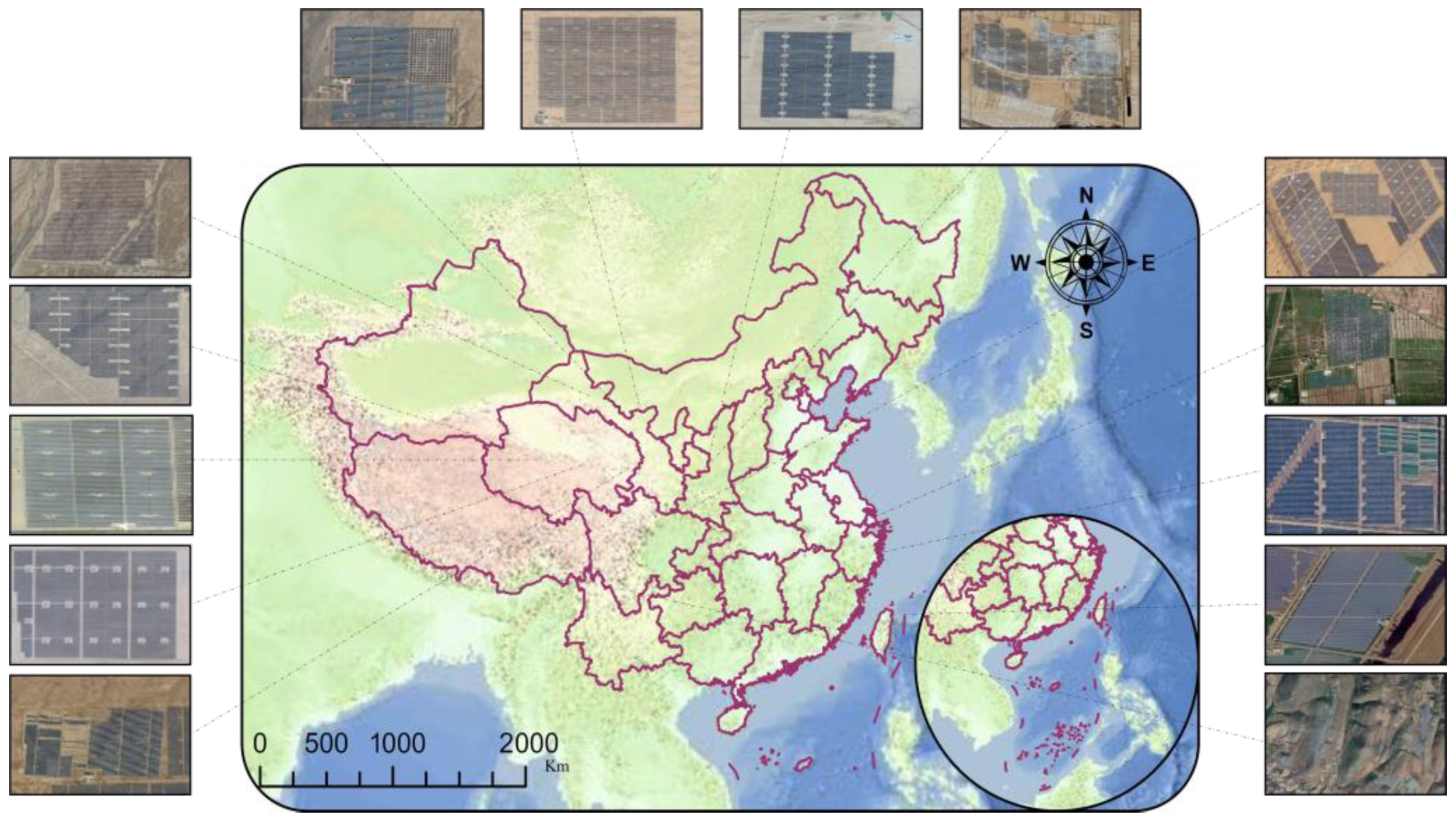
Commonly utilized PV panel statistics rely on medium-resolution remote sensing imagery, which is only able to identify the location of PV panels and is unable to fulfill the requirements of quantitative statistics. To address this issue, this paper employs high-resolution aerial imagery to accurately detect and extract PV panels and substations in a complex environmental scene. The aerial imagery data utilized in the dataset were collected from various provinces in China, such as Xinjiang, Gansu, Mongolia, Ningxia, and Sichuan. Figure 1 displays high-resolution aerial images of PV panels captured by large aerial cameras, with resolutions varying from 0.15 to 0.3 m due to different equipment used in various regions and flight altitudes. The significant differences in solar incidence angles between regions and sampling times result in structural differences in the images, which poses a greater challenge for the effective extraction of PV panels.

To construct the model, this paper adopts a semi-supervised approach considering the time, cost, and complexity of the application. Although the semi-supervised training sample balance requirement is reduced, a combination of labeled and unlabeled dataset construction is still necessary to optimize the key features that the model perceives during the unsupervised training process. The collected images are divided into four copies for vectorization, where the fully supervised training process only learns the features of the first sample and some of the features of the other two samples. Unsupervised comparative learning can only obtain the features of the last sample to check if the features extracted by unsupervised training can be effectively generalized to a similar image segmentation process.

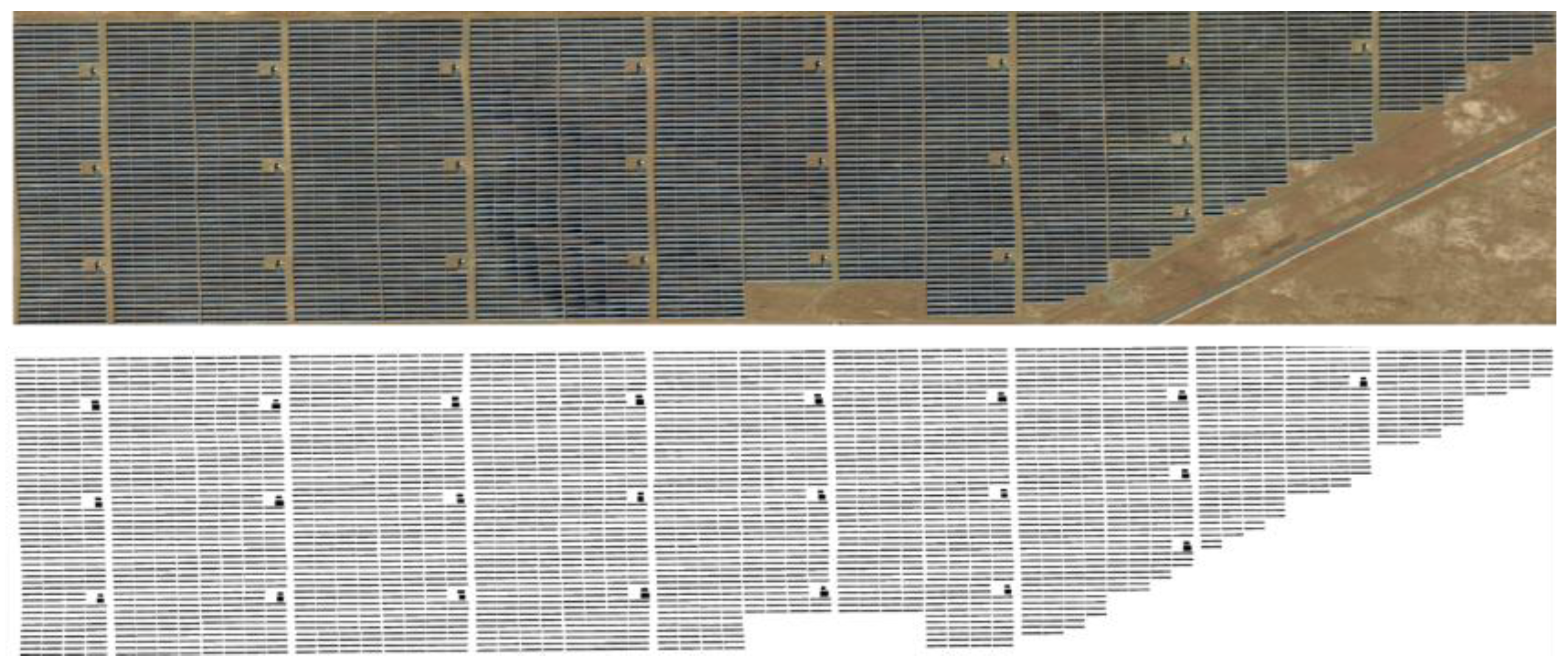
In Figure 2, a detailed manual vector sample of a Hainan mudflat PV plant is presented and accurately labeled with the precise location and attributes of each PV panel and substation. A total of 15 annotated aerial remote sensing images and corresponding labels of similar complexity are included, alongside over 40 unlabeled aerial images, forming a large-scale, high-precision, semi-supervised training dataset optimized for machine/deep learning applications. All images were collected from multiple geographic regions using heterogeneous sensors and stored in three-channel (RGB) format. To preserve visual and morphological details, each image was cropped into 512 × 512 patches while maintaining their original resolution. The spatial distribution, sensor types, and sample proportions of the dataset are systematically summarized in the accompanying

Table 1. Distribution and statistics of photovoltaic datasets.

Area	Quantity	Background
Hainan	105	Sandy land
Hebei	625	Grass
Ningxia	765	Sandy land
Jilin	210	Saline–alkali lands
Sichuan	1260	Mountains, Towns
Qinghai	432	Sandy land, Saline–alkali lands, Mudflat
Inner Mongolia	512	Sandy land, Saline–alkali lands
Xinjiang	391	Sandy land, Saline–alkali lands
Jiangsu	235	Mudflat, Towns
Total	4535	/

.

4. Models and Methods

The model proposed in this paper has two stages: the first stage constructs an agent task based on individual recognition (unsupervised), and the second stage constructs a mapping task based on sample images and labels (fully supervised). This section focuses on our approach to model pre-training, model optimization, and adaptive weighting of the loss function. Since the task is based on multi-category semantic segmentation in complex scenes, we use one-hot encoding to reconstruct the labels. This is an image coding method that converts single-channel multi-valued samples into multi-channel binary samples. Additionally, we normalize the dataset using a z-score data normalization method, transforming it into an input with a mean of 0 and a variance of 1.

4.1. JSWPVI Backbone Network Pre-Training

Convolutional neural networks are widely believed to consist of a backbone network, neck layer, and classification head. The backbone network plays a crucial role in feature extraction from images and facilitates the migration of computer vision class models [34].

To obtain image features covering multiple types of PV panels and substations, this paper employs a backbone network trained on numerous unlabeled samples through pre-training with individual recognition. Specifically, we refer to the MOCO algorithm, an unsupervised pre-training process that leverages contrast learning to construct an individual recognition agent task for pre-training [44,45].

Figure 3 demonstrates the model’s ability to randomly select samples $x$ from an extensive collection of unsupervised image slices, and utilize sample augmentation (random color distortion, random Gaussian blur) to generate $x^q$ and $x_0^k$ respectively. Secondly, $n$ remaining samples are randomly selected to construct the queue $x^k=\{x_0^k, x_1^k, \dots , x_n^k\}$, thus obtaining a queue containing a total of $n+1$ samples; finally, the model backbone network is used as the feature extraction layer, and MLP (multilayer perceptron) is used to fuse multidimensional features to obtain the output of continuous feature values. Among them, $x^k$ and $x^q$ use the same coding structure, $x^k$ and $x^q$ correspond to the encoders defined as $E^k$ and $E^q$, and the parameters of the encoders are defined as $P(E^k)$ and $P(E^q)$, respectively. The sample queue approach can reduce the GPU memory requirement, but it also leads to the fact that the convolution parameters of the computational queue cannot be optimized by backpropagation. In order to properly train the model with smooth gradient changes and thus reduce the pre-training bias of the backbone network, the gradient values of $E^k$ are experimentally removed and $P(E^k)=0.99\times P(E^q)$ is used to update the parameter values.

It should be noted that the model uses a particular loss function $L_{InfoNCE}$ to implement the comparison of successive eigenvalues of the model to prompt unsupervised pre-training to efficiently optimize the JSWPVI backbone network, whose expression is shown in Equation (1):

$$L_{InfoNCE}=-\log {\displaystyle \frac{\exp (q\cdot k_{+}/\tau )}{\exp (q\cdot k_i/\tau )}}$$

(1)

In Equation (1), $q$ and $k$ are the continuous eigenvalues computed by $x^q$ and $x^k$, respectively; $k_{+}$ represents the continuous eigenvalues computed by $x_0^k$, which is the only positive sample in the individual recognition task and $\tau$ is a temperature parameter to control the distribution shape of the continuous eigenvalues—the larger the value of $\tau$, the smoother the distribution of the eigenvalues, and for the opposite, the distribution is more concentrated. With this loss function, the model can reduce the distance between similar samples while increasing the distance between different samples, thus realizing unsupervised pre-training of the JSWPVI backbone network.

4.2. JSWPVI Construction and Fully Supervised Retraining

In the previous section, we delved into the pre-training of the JSWPVI’s backbone network to tackle the issue of insufficient labeled data for PV panels and substations. Now, we turn our attention to the construction of JSWPVI as a whole and its fully supervised retraining process.

Despite the effectiveness of pre-training in feature extraction, a considerable amount of redundancy still exists in low-dimensional information, which renders the features less useful when the same weights are assigned. Moreover, because the model is based on pre-training for individual recognition, the obtained features differ somewhat from those in semantic segmentation. Transitioning from pre-training parameters to semantic segmentation training presents challenges in finding the best learning rate for optimization since the learning rate can vary significantly. Deep learning models have strong black-box characteristics, making it challenging to compare the differences between features in the above two training models. To address these challenges, we propose two improvements to the up-sampling structure. First, we improve the initial learning rate by using variable hyperparameters and optimizing them with a simulated annealing algorithm to automatically find the optimal learning rate when the model features are fused. Second, we link the up-sampling and down-sampling by long connections in the up-sampling process structure and construct the “Spatial and Channel Weight Adaptive Model” (SCWA) structure to automatically assign feature map weights to reduce the difference between semantic segmentation and individual recognition tasks (check Appendix A for more details).

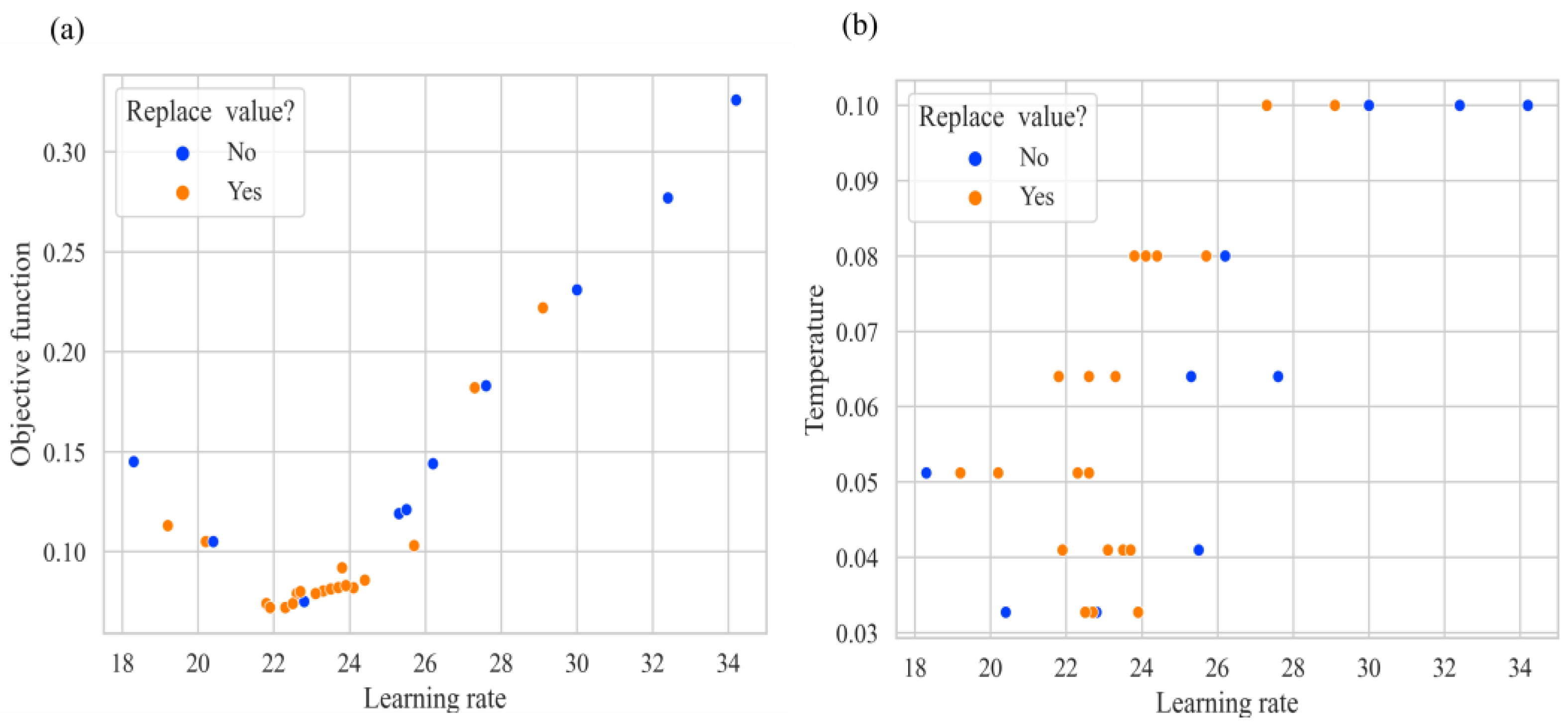
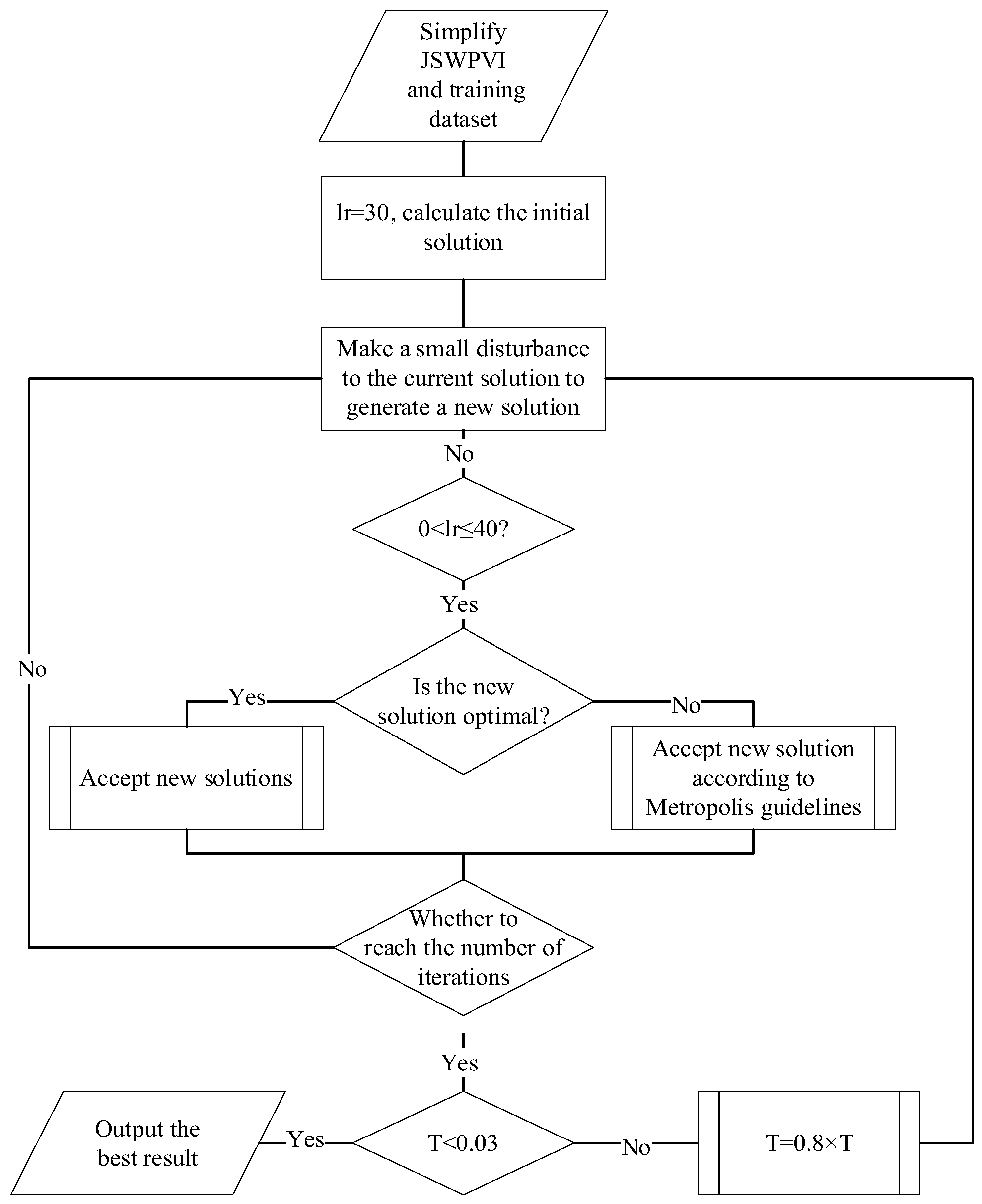
Because pre-trained features obtained through contrast learning and fully supervised features exhibit variability, the traditional learning rate hyperparameters introduce uncertainty. In the MOCO algorithm, Kai-Ming He et al. [22] demonstrated that the optimal learning rate (lr) for an agent task based on individual recognition, migrating to a downstream application, can even reach an incredible 30. To automatically search for the optimal learning rate, we use a simulated annealing algorithm for adaptive estimation. The simulated annealing algorithm (SA) is a general probabilistic algorithm commonly used to find the approximate optimal solution in a large search space in a certain time. SA avoids the trap of locally optimal solutions by setting a high initial temperature (T), which allows the model to accept poorly performing values initially. The overall flow of the simulated annealing algorithm in this paper is shown in Figure 4.

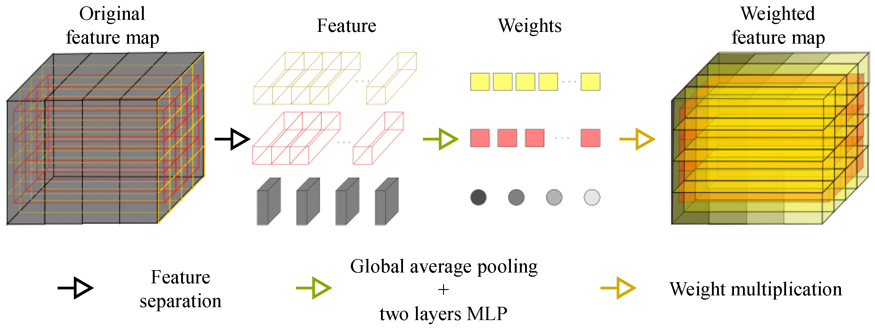
To reduce the discrepancy between semantic segmentation and individual recognition tasks, a feature map weight extraction algorithm named “Spatial and Channel Weight Adaptive Model” (SCWA) is constructed by stacking up-sampled and down-sampled feature maps. The SCWA receives the original feature map as input, separates the features based on location and channel, performs global average pooling to reduce the high-dimensional features to low-dimensional weights, and finally multiplies the weights back to the original feature map according to the location of the feature extraction, creating a weighted feature map. The detailed structure and computational flow of the SCWA are illustrated in Figure 5. The feature separation simplifies the weight calculation, with the original feature map’s size being H×W×C, the yellow and red spatial features’ size being H/4W/4C×(16 + 9), and the channel features’ size being H×W×1×C. The SCWA uses global average pooling to generate a neuron of size 1 × 1 for each feature to measure its importance to the feature map, and two additional layers of MLP structure (using Softmax nonlinear activation) are added to increase the nonlinear representation of the weights. The computed weights are then multiplied with the original feature maps to obtain the weighted feature maps, realizing the automatic assignment of spatial and channel weights and reducing variability in pre-trained features’ migration from contrast learning to a fully supervised process.

The number of parameters and structure rationality of convolutional neural networks often determine the model’s inference ability and output accuracy. However, a large number of parameters can lead to problems such as overfitting and parameter redundancy, greatly reducing the model’s inference speed. Therefore, a complex model structure does not necessarily produce better prediction results. In order to accelerate the model’s iteration and prediction, we used only a bottleneck layer structure similar to U-Net and a classification head. The complete JSWPVI (shown in Figure 6) adopts an autoencoder structure and achieves a fusion of low-dimensional and high-dimensional features by stacking down-sampling and up-sampling features. This expands contextual information and retains the most important multi-scale information for semantic segmentation tasks, improving the semantic segmentation accuracy of PV panels and substations, while also possessing fast inference speed.

4.3. Constructing a Fully Supervised Training Error Function

To better capture unlabeled features, the experiments did not filter for pure background labels, resulting in a further exacerbation of the already imbalanced sample distribution between the background, PV panel, and substation. Based on the available labeled samples, the three categories account for 87.31%, 12.57%, and 0.12% of the samples, respectively. However, the extremely uneven distribution of category pixels creates a significant classification bias issue for the model, making it unsuitable for multi-category target extraction. To tackle this problem, two error functions were experimentally computed. The first is the weighted cross-entropy error, which measures whether each pixel is correctly classified relative to the others. The second is an improved version of the Tversky function, designed to automatically balance multi-classified samples. These two loss functions can measure the extraction accuracy of PV panels and substations in terms of pixel classification accuracy and the percentage of true and false positives.

The expression for the weighted cross-entropy error is as follows:

$$L_{Cross-Entropy}=-{\displaystyle \sum _{i=1}^k{w}_i{\widehat{y}}_i\ln y_i}$$

(2)

In Equation (2), $k$ represents the class of the sample, $w_i$ is the weight of the sample in each class, $y_i$ is the label, and ${\widehat{y}}_i$ is the model classification result. The Tversky loss function is a simple and efficient loss function for the self-balancing of binary samples [46], and we improve the construction of the Tversky function to address the problem of unbalanced samples in multiple classes, and its expression is as follows:

$$\begin{array}{l}T{P}_k={\displaystyle \sum _{k=1}^{m_0}{\displaystyle \sum _{i=1}^n{P}_{x_i}^k\times P_{{\widehat{x}}_i}^k}}\\ F{P}_k={\displaystyle \sum _{i=1}^n({\displaystyle \sum _{j=1}^{m_1}{P}_{x_i}^j}\times {\displaystyle \sum _{k=1}^{m_0}{P}_{{\widehat{x}}_i}^k}})\\ F{N}_k={\displaystyle \sum _{i=1}^n({\displaystyle \sum _{k=1}^{m_0}{P}_{{\widehat{x}}_i}^k}\times {\displaystyle \sum _{j=1}^{m_1}{P}_{x_i}^j})}\end{array}$$

(3)

$$L_{Cross-Entropy}=-{\displaystyle \sum _{i=1}^k{w}_i{\widehat{y}}_i\ln y_i}\left\{\begin{array}{l}\begin{array}{ll}{L}_{Tversky}=1-{\displaystyle \sum _{k=1}^{m_0}\frac{T{P}_k}{(T{P}_k+\beta F{P}_k+(1-\beta )F{N}_k+S)m_0}}& \hspace{1em}\hspace{1em}{\displaystyle \sum _{k=1}^{n}T{P}_k>0}\\ \hspace{1em}\hspace{1em}{L}_{Tversky}={\displaystyle \sum _{k=1}^{m_0}\frac{F{P}_k+F{N}_k}{(M\times N)m_0}}& {\displaystyle \sum _{k=1}^{n}T{P}_k=0}\end{array}\end{array}\right.$$

(4)

In Equations (3) and (4), $m_0$ is the image channel of interest after one-hot encoding; $m_1$ is the remaining channels included in the one-hot encoding; $n$ is the number of pixels of the image; $[P_x,P_{\widehat{x}}]$ corresponds to the predicted classification and labeled classification, respectively; $k$ and $j$ represent the $k$th channel and jth channel of the image, respectively; $\beta$ is the weight balance parameter; $[T{P}_k,F{P}_k,F{N}_k]$ denotes the true positive rate, false positive rate, and false negative rate of the attention channel, respectively; $[M,N]$ is the training sample size of the image; $L_{Tversky}$ is the loss value; $S$ is the factor that prevents the denominator from proceeding to zero.

The $L_{Cross-Entropy}$ error is widely used as a loss function in the field of deep learning, and many mature optimization algorithms can be used to accelerate its training process. However, it still cannot effectively handle extremely imbalanced datasets. On the other hand, the $L_{Tversky}$ error adopts a more suitable approach for imbalanced samples and can achieve a better balance between accuracy and recall. However, the optimization goals of the two loss functions are different, and both are non-convex functions that can easily get stuck in locally optimal solutions. To more effectively combine the two loss functions, we have drawn on the ideas of multi-task learning and multi-objective optimization and applied automatic weighting of the loss functions in the same model to achieve Pareto optimality [47,48], as detailed in Algorithm 1.

Algorithm 1 Automatic weighting of loss functions

Inputs: [loss1, loss2], Model, Learning Rate:

Output: Model

1: function $(Gra{d}_{o}pt)[loss1,loss2],Model,LearningRate$      % CALCULATE THE GRADIENT OF ALL LOSS FUNCTIONS

2:   $grad1,grad2\leftarrow \nabla loss1,\nabla loss2$      % FAN OF THE GRADIENT OF THE LOSS FUNCTION

3:   $norm1,norm2\leftarrow {\displaystyle \frac{grad1-gr\overline{a}d1}{\sigma }},{\displaystyle \frac{grad2-gr\overline{a}d2}{\sigma }},$ $\sigma =\sqrt{{\displaystyle \frac{1}{n}}}{\displaystyle {\sum }_{i=1}^1{(gra{d}_i,-gr\overline{a}{d}_i)}^2}$      % AVERAGE OF THE NORM OF THE GRADIENT OF THE LOSS FUNCTION

4:   $std1,std2\leftarrow STD(norm1),STD(norm2)$      % DEVIATION FROM THE NORM OF THE GRADIENT OF THE LOSS FUNCTION

5:   $dev1,dev2\leftarrow {\displaystyle \frac{norm1-no\overline{r}m1}{std1}},{\displaystyle \frac{norm2-no\overline{r}m2}{std2}}$      % CALCULATE THE WEIGHTS ACCORDING TO THE DEGREE OF DEVIATION

6:   $weight1,weight2\leftarrow \exp (-dev1),\exp (-dev2)$      % NORMALISATION OF THE OBTAINED WEIGHTS

7:   for $i,j$ in $ZIP(weight1,weight2)$ do  8:    $i,j$$\leftarrow$$i/{\displaystyle \sum weight1,j/{\displaystyle \sum weight2}}$  9:   end for      % CALCULATE THE WEIGHTED GRADIENT  10:    $grad1,grad2\leftarrow weightl?grad1,weight2?grad2$      % UPDATE THE MODEL PARAMETERS ACCORDING TO THE GRADIENT  11:   for $param,gradinZIP(Model.parameters(),grad1,grad2)$ do  12:   $param\leftarrow LearningRate\times grad$  13:   end for  14:   end function

Through the aforementioned pseudocode, we have calculated various indicators such as gradients, gradient norms, mean and standard deviation of gradient norms, and deviation of gradient norms for each loss function. Using these indicators, we obtained weights for each loss function and computed the weighted average gradient, which we then used to update the model parameters. This approach is a multi-task learning method based on multi-objective optimization. Compared to the weighted linear combination of multiple loss functions, this method eliminates the process of weight optimization and can maintain stability even when the loss functions are nonlinearly related or have conflicting optimization goals (such as recall and precision), thereby achieving Pareto-optimal solutions. Furthermore, it supports the JSWPVI to perform fully supervised semantic segmentation retraining under sample imbalance conditions, providing necessary conditions for model convergence.

4.4. JSWPVI Results Post-Filtering

Due to various limitations such as technical ability, sample size, and image and label quality, discrepancies may exist between model predictions and ground truth in semantic segmentation tasks. Typically, these discrepancies are concentrated around the edges of images. However, in the case of the JSWPVI, model predictions are relatively accurate at the edges, but some unexplainable noises in the interior may affect the extraction of PV panel points and area estimation. Therefore, it is necessary to adopt effective filtering methods to eliminate these noises, improve model predictions, and make them more suitable for statistical and practical applications.

Common denoising methods, such as Gaussian filtering, image closing operations, and threshold filtering, only consider the value range or spatial domain of the image, which may cause blurring of the information for complete edge prediction. In addition, improper parameter settings may reduce the credibility of the results. To achieve non-edge image filtering focused on model prediction, the guided filter algorithm is used to optimize the segmentation results using aerial photographs as guidance [49]. The guided filter is a locally linear model-based image filtering algorithm, which filters the input image and a guidance image to retain the structural information of the guidance image while removing noise and details. Specifically, the guided filter performs linear regression on the neighborhood of each pixel to obtain the filtering coefficients of that pixel, and then uses these coefficients to perform weighted averaging on the pixels within the neighborhood to obtain the output value of that pixel. Compared with other filtering algorithms, guided filtering has a better edge preservation effect and considers both the value range and spatial domain of the image, which can preserve the details of the image while removing noise. Therefore, it has been widely used in the field of computer vision and image processing. The detailed description is as follows:

$$q_i=\sum _j{W}_{ij}(I){\widehat{y}}_j$$

(5)

In Equation (5), $I$ is the guided image, which represents the high-resolution aerial remote sensing image input of the JSWPVI, ${\widehat{y}}_i$ is the segmentation image representing the output of the model, and $q_i$ represents the result after the guided filtering. $W_{ij}$ represents the filter kernel coupled with the guided image $I$, and the filter is linear for $\widehat{y}$. An important assumption exists for the guided filtering, as shown in Equation (6):

$$q_i=a_k{I}_i+b_k,i\in w_k$$

(6)

Equation (6) assumes that for a given deterministic window of radius $r$ there is a unique constant coefficient between $a_k$ and $b_k$. This assumption ensures the same edge retention between the guided image $I$ and the output image $\widehat{y}$ in the local region. It is also assumed that the non-edged and unsmooth region of the image is the noise $n$, so it can be assumed that $\widehat{y}$ is the result of the superposition of $q_i$ and $n$, and therefore Equation (7) is derived as follows:

$$q_i={\widehat{y}}_i-n$$

(7)

For each filter window, the algorithm can be optimized using a least squares algorithm as shown in Equations (8) and (9):

$$argmin\sum _{i\in w_k}{\left(a_k{I}_i+b_k-{\widehat{y}}_i\right)}^2$$

(8)

$$E\left(a_k,b_k\right)=\sum _{i\in w_k}\left({\left(a_k{I}_i+b_k-{\widehat{y}}_i\right)}^2+ϵa_k^2\right)$$

(9)

Equation (9) is based on Equation (8) with the introduction of the regularization parameter $ϵ$, which aims to avoid the overall deviation of the model caused by too large $a_k$, and is optimized by the ridge regression algorithm. Overall, guided filtering is an optimized improvement of bilateral filtering, using the high-resolution aerial photography image as the guided image and the PV panel segmentation result (probability value without using the activation function) as the image to be filtered, which can effectively improve the quality of the segmentation result.

5. Experiment and Analysis

This section primarily discusses the process and parameter setting of using the simulated annealing algorithm to determine optimal learning rates. Additionally, we conducted an ablation experiment on the SCWA structure and compared JSWPVI with DeepLabV3+.

5.1. Indicator Introduction

To evaluate the performance of the proposed model in PV panel segmentation tasks, three widely adopted metrics were employed: the Kappa coefficient, F1-score, and Intersection over Union (IoU). These metrics, extensively utilized in remote sensing image segmentation, assess model effectiveness from the perspectives of classification consistency, precision-recall balance, and spatial overlap accuracy, respectively. The mathematical formulations for Kappa Coefficient are as follows:

$$Kappa={\displaystyle \frac{p_0-p_e}{1-p_e}}$$

(10)

Among them, $p_0$ is observation consistency and $p_e$ is expected consistency. In photovoltaic mapping, Kappa reflects the overall classification consistency of the model between photovoltaic panels and background.

The F1-score is the harmonic mean of precision and recall, serving as a balanced metric to evaluate the model’s classification performance on the positive class. The formula is defined as follows:

$$F1=2\cdot {\displaystyle \frac{Precision\cdot Recall}{Precision+Recall}}$$

(11)

The IoU is a standard metric for evaluating pixel-level segmentation accuracy by quantifying the overlap between predicted segmentation regions and ground truth regions. It is calculated as follows:

$$\mathrm{IoU}={\displaystyle \frac{TP}{TP+FP+FN}}$$

(12)

5.2. Comparative Experiments

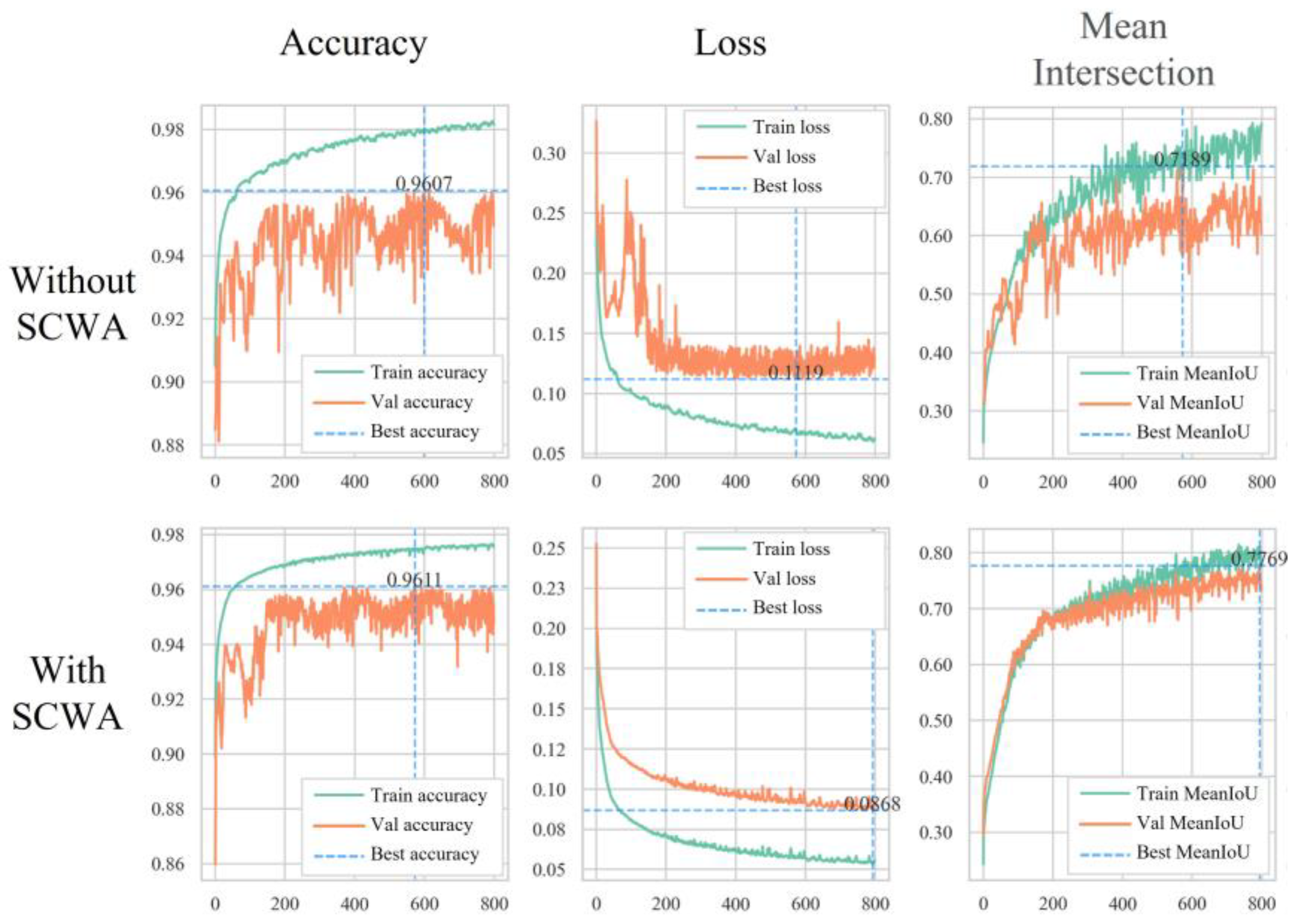
To authenticate the JSWPVI’s efficacy, we employed the high-resolution aerial remote sensing dataset of PV panels and substations, explicated in Section 2, for training and validation. In addition, we performed ablation experiments to compare the model’s performance with and without the SCWA module. Figure 7 and

Table 2. Ablation control experiments were conducted on SCWA structures, where the JSWPVI-SCWA refers to the JSWPVI with the SCWA structure eliminated.

Methods	Kappa	F1-Score	PA	mIoU
JSWPVI-SCWA	0.928	0.875	0.911	0.777
JSWPVI	0.909	0.841	0.894	0.751

present the results of JSWPVI’s training and validation concerning the SCWA ablation experiments. Three parameters are mainly visualized, namely accuracy, loss, and mean intersection. The green and yellow curves denote the variations in the training and validation sets, respectively, while the blue dashed lines indicate the optimal values acquired from the validation set. As depicted in Figure 7, the JSWPVI backbone network is pre-trained and can achieve faster convergence on the validation set, irrespective of the SCWA structure’s presence. However, due to the superfluous deep learning parameters and intricate migration features, the JSWPVI without SCWA exhibits considerable oscillations, which are likely due to the large learning rate’s difficulty in achieving convergence. This issue can be resolved by optimizing the decay rate of the learning rate. On the other hand, the SCWA module requires fewer parameters and less computational power. Furthermore, the ablation comparison experiment with 800 iterations takes almost the same time.

In summary, the JSWPVI, equipped with the SCWA mechanism, compresses redundant information and enhances the confidence level of foreground targets (PV panels and substations), thereby improving the accuracy of discrimination results. Consequently, SCWA facilitates better adaptation of the model to pre-training weights obtained from individual recognition. It effectively extracts PV panels and substations from high-resolution aerial remote sensing images.

To further verify the accuracy of the results obtained for the JSWPVI PV panel and substation extraction, we conducted a comparison using the DeepLabV3+ model (backbone network: ResNet50) [19]. The prediction set images were utilized as the benchmark for model inference. DeepLabV3+ is a well-known semantic segmentation model widely employed in remote sensing target extraction tasks, with a Cityscapes dataset and an 82.1% cross-merge ratio achievement. In this study, DeepLabV3+ weights were constructed using fully supervised training and MOCO pre-training methods, respectively, and compared with JSWPVI to demonstrate the model’s effectiveness.

Furthermore, to rigorously evaluate the effectiveness of the semi-supervised method proposed in this study, we introduced UniMatch, an additional semi-supervised approach, as a benchmark. UniMatch has demonstrated State-of-the-Art (SOTA) performance on the Pascal VOC 2012, Cityscapes, and COCO datasets and has been successfully applied to tasks such as change detection in remote sensing imagery. In this study, UniMatch was trained under identical dataset configurations to validate the proposed model’s efficacy.

JSWPVI was mainly compared with DeepLabV3+ in this study, as the latter has been widely used in various classification scenarios, exhibiting excellent performance and high confidence with its pre-trained weights, making it suitable for this comparative experiment. In this research, there were two ways to train the DeepLabV3+ model: the first one was to fine-tune the pre-trained weights of ImageNet (F-DeepLabV3+), and the second one was to fine-tune the self-supervised pre-trained weights used in this paper (P-DeepLabV3+). The fine-tuning process included the use of artificially produced aerial PV panels and substation samples.

Figure 8 presents several prediction results labeled A–E, which were obtained under varying geographic regions, sensors, altitudes, and weather conditions. Example A illustrates a regular distribution of PV panels, while B and C contain interfering objects that resemble PV panel features. In contrast to A–C, the scene in D exhibits significant differences between PV panels and the background, and the PV panel types in this area were not included in the training samples. Example E demonstrates the detection of PV panels in a distributed scenario.

A comparison of four models across different scenes reveals that F-DeepLabV3+ fails to separate adjacent PV panels effectively, resulting in classification errors, blurred boundaries, and mixed information in the segmentation outputs. Compared to F-DeepLabV3+, which uses ImageNet pre-trained weights, the JSWPVI and P-DeepLabV3+ models adopt a pre-training strategy based on individual identification. This approach yields more reliable extraction results for both PV panels and substations, as shown in the statistical summary in

Table 3. The comparison between JSWPVI and DeepLabV3+ models is as follows. F-DeepLabV3+ was trained using only labeled samples, while P-DeepLabV3+ utilized a large number of unlabeled samples for backbone network pre-training and fine-tuning with labeled samples.

Methods	Kappa	F1-Score	PA	mIoU
JSWPVI	0.928	0.875	0.911	0.777
F-DeepLab V3+	0.744	0.711	0.859	0.597
P-DeepLab V3+	0.911	0.842	0.901	0.759
UniMatch	0.885	0.821	0.889	0.736

. The performance of UniMatch falls between P-DeepLabV3+ and JSWPVI. Notably, UniMatch produces very smooth outputs, especially in scenes A–C. However, its performance degrades at the edges and in identifying substations. This may be attributed to its consistency regularization strategy, which effectively reduces pseudo-label noise and leads to more coherent and smooth predictions.

Overall, the baseline results are not surprising, as manual annotations in panoramic remote sensing segmentation often contain substantial errors. This makes it challenging to build effective pre-trained weights in a fully supervised manner. In addition, ImageNet pre-trained weights are derived from conventional photographic RGB images, which differ significantly from remote sensing imagery in terms of subject matter and spectral characteristics. Although ImageNet pre-training can improve recognition accuracy to some extent, its overall optimization effectiveness is often limited, making it difficult to achieve good generalizability.

In summary, the comparison showed the following: (1) JSWPVI reduces voids in PV panel extraction and improves the smoothness of edges. The SCWA module adaptively assigns weights to guide the model’s attention to critical features, and the overall prediction of the model does not change significantly due to minor error perturbations, thereby demonstrating better adaptability in complex scenes. (2) The addition of backbone network pre-training improves the model, significantly enhancing the edge accuracy of extracted PV panels. It can significantly improve the independence between PV panels when the image seams are not clear and maintain good generalization ability in some images with large differences in morphological features. The extracted PV panels and substations will rarely exhibit errors such as voids and interruptions, thus ensuring the accuracy of extraction, which is crucial for area and quantity statistics.

5.3. Model Application and Result Filtering

However, even though the JSWPVI technique is adept at extracting PV panel data from images, the inconsistent panel sizes and minuscule gaps between them could result in certain disparities between the data annotation and the actual situation. These factors undoubtedly befuddle the model and impede its ability to recognize the PV panels, leading to inevitable non-edge noise in the model predictions and voids in the results. To tackle this problem, we employed a guided filtering algorithm to optimize the prediction outcomes, reduce numerical voids in the extraction results, and rectify the image distortion caused by noise. Figure 9 displays a comparison between the outcomes before and after the guided filtering operation. By exploiting the gradient information of the input image, the noise in both the zero and value domains is effectively suppressed, and the independence of the PV panels with small gaps is preserved. Following the filtering process, the noise level of the PV panels is considerably decreased, and the extraction outcomes are smoother.

To further evaluate the generalization ability of the model in different scenarios, we carefully examined the images of the test set and divided them into five landscapes based on their environment, namely towns, mountains, deserts, beaches, and saline–alkali lands. Considering that distributed photovoltaic panels mainly exist in urban areas and do not have obvious characteristics of substations, we only evaluated the recognition accuracy of photovoltaic panels in urban areas. The recognition results are shown in

Table 4. Comparison of accuracy between PV panels and substations in different scenarios.

Methods	PA		mIoU
	Panels	Substations	Panels	Substations
Town	0.915	-	0.761	-
Mountain	0.924	0.946	0.786	0.771
Desert	0.978	0.968	0.805	0.782
Beache	0.964	0.910	0.793	0.765
Saline land	0.937	0.859	0.768	0.757

. Although different regions come from different collection devices, the model still shows high reliability in terms of PA and mIoU, especially in mountain and desert scenes. The model’s predictions are highly consistent with the true values. However, in urban and saline–alkali areas, the prediction accuracy of the model significantly decreases. After examining the images, we found that the number of samples in saline–alkali lands is sparse, and the characteristics of the substation are relatively consistent with the background, which increases the difficulty of model recognition. In urban scenarios, we found that the loss of accuracy mainly comes from two aspects. Firstly, there is a large number of thermal insulation panels and glass with similar spectral and shape characteristics on the roofs of cities, and similar objects do not exist in other areas, resulting in incorrect recognition by the model. Additionally, since distributed photovoltaics are usually managed by individuals, some photovoltaic panels may experience tilting due to poor management, resulting in changes in their morphological characteristics and missed detections by the model.

6. Conclusions

As the cost of PV systems decreases, the use of solar power generation will become more common in the coming decades. To better understand the completion of PV power plants, and support power generation forecasting and carbon emission statistics, collecting statistical data on the quantity and location of PV panels is helpful. However, the construction of PV power plants often occurs in harsh environments such as town, mountains, beaches, deserts, and saline–alkali land, which makes it challenging to accurately determine the construction area, quality, and quantity using manual methods. Therefore, aerial remote sensing imagery, with its high resolution and large coverage area, has become one of the main means of PV statistics and detection. Combined with deep learning algorithms, it can effectively and with a high quality obtain the status of PV power plants. However, the large number of aerial remote sensing images related to the construction of PV power plants, the small number of effectively annotated images, and the difficulty of supporting complex model training make it challenging.

This article proposes an efficient and high-quality sample construction process based on aerial photos to address the challenges mentioned above. After multiple attempts and iterative updates, a comprehensive dataset with supervised and unsupervised data was generated, and a standardized and normalized sample database was constructed. Then, we pre-trained the unsupervised backbone network with a large number of unlabeled samples and optimized the supervised model with a small number of labeled samples based on it. To address the problem of a non-fixed learning rate when transferring unsupervised pre-training weights, we used the simulated annealing algorithm to iteratively optimize the learning rate and proposed SCWA to construct adaptive feature selection and weighting structures to alleviate the differences between pre-training tasks and fully supervised tasks. To deal with the problem of negative sample balance and the possibility of newly labeled samples being added to the optimization process at any time, we also calculated the gradients of $L_{Cross-Entropy}$ and $L_{Tversky}$ loss functions and directly optimized the model parameters using the loss function gradient weighting method based on the deviation from their corresponding two-norm weights. Finally, we proposed the JSWPVI method, which is effective for extracting and counting PV panels and substations from high-resolution aerial photos and exhibits strong generalization ability in both centralized and distributed scenarios. With a small number of samples, good segmentation results can be obtained. To overcome the problems of spatial and value domain noise in the segmentation results, we combined guided filtering to improve the extraction results. Overall, the JSWPVI method can effectively determine the quantity and area of PV panels and substations in complex environments, providing a valuable reference for PV system construction and data updating.