Population and Landslide Risk Evolution in Long Time Series: Case Study of the Valencian Community (1920–2021)

Abstract

Assessing the size and situation of the population exposed to natural hazards is a fundamental step in addressing natural hazard management and emergency planning. Although much progress has been made in recent years in population geolocation by competent public bodies, gathering historical data beyond the present century to learn about the sequential evolution the affected population has experienced remains a difficult task. The recent publication of a historical population grid with adequate resolution allows progress to be made in resolving this problem. This paper is based on these data together with a map of landslide susceptibility in the study area and on the abundant resources provided by the Spanish Cadastre on dates of construction, surface area, and location of built plots. The size of the residential area built in the risk zone and its affected population was calculated since the early 1900s and with a decennial sequence. The risk to the population has been found to be stable or decreasing slightly over the entire historical series in the study area. However, the intensive tourism in some coastal municipalities in the north of Alicante has led to the construction of holiday homes in unsuitable locations in mountainous areas and with it an appreciable increase in risk.

1. Introduction

In recent years, society has seen an increase in damage caused by natural hazards. Floods stand out in particular for their visibility, extent, intensity, and frequency, in which climate change is presented as a primary triggering agent. In the case of landslides, with unequal influence but marked by unprecedented meteorological events [1,2,3], one important factor is the increased exposure to risk of susceptible elements: population, buildings, and infrastructure [4].

One of the most important aspects of these types of events is the prior assessment of the potential damage that may be caused taking into consideration the vulnerability of the elements at risk. Different dimensions of this vulnerability are often taken into account and there can be of many types of them, although the social, personal, and structural are those generally addressed [5,6] and linked together [5,7,8]. Integrated approaches to evaluation are increasingly being addressed as one would expect [9,10] although they require a highly detailed quantitative evaluation. Indeed, the variety of elements that are subject to damage and loss together and their different characteristics (e.g., buildings, public works, people) require complex analysis, so such studies are not abundant [11,12,13].

It is common for only two areas of work to be taken into account, namely physical and social. Attempts have been made to establish empirical relationships with regard to property damage between the intensity of the process and the type and quantity of elements exposed to value the estimated loss, usually in monetary units [8,14,15,16,17,18,19,20,21].

In the other area of work, on social damage, research has focused on how affected societies adapt to these events, and how to cope with their consequences [22,23,24]. The study by [25] on long-term social impacts in mountain communities is of note. Work has also been conducted to assess the relationship between the occurrence of a process and the damage caused to people by defining curves between the two variables [26,27]. Human activity itself, by causing changes in soil characteristics, is clearly a trigger for these processes in the most inhabited areas, leading to a greater impact on the population [28].

All of these studies are generally based on historical data on risky events that affected the population and collected in specific inventories [29,30]. Logically, these historical inventories are often insufficient and incomplete, which means that the probabilistic calculation has often been based on expert analysis [11]. Consequently, very different approaches need to be adequately addressed to tackle these complex problems [9]. A significant number of data types with different ranges and units (material, personal, social) must also be taken into account to estimate the value of the damage caused if quantitative risk analysis is used [31,32,33,34,35].

An accurate assessment of the number of people present at a given time and place is a necessary first step, as it is crucial to develop a consistent emergency plan. Knowing as precisely as possible the location of the potentially exposed population is essential to ensure emergency plan efficiency and to reduce associated costs related to rescue and community recovery [36,37,38,39]. According to [40], locating the population at risk should be the first step to mitigating personal damage and reducing casualties.

Their results must be accompanied by an analysis of the local situation, developing a system for assessing the available social, economic, and health care fabric [41]. Urban resilience is generally particularly dependent on emergency response along with its potential for immediate recovery and reconstruction after any catastrophic event [42]. Civil society must be able to prepare, anticipate, preserve, absorb, respond, resist, recover, mitigate, learn, and adapt to these situations [43].

Population distribution data for large areas and in broad historical series are essential first to learn how the risk has evolved, the places where it is most intensely concentrated, and also to provide adequate criteria to optimise territorial management and prevent damage [3]. Significant differences in population density are expected, especially in larger study areas where there may be different types of use (urban concentration or rural or holiday dispersion). This study’s goal is to analyse the historical series of the geolocalised population affected by these events to establish variation patterns and define areas of preferential application of territorial policies that minimise possible damage caused by landslides.

The aim of this paper is to define the preferred areas of action to prevent social damage, to the population in particular, caused by landslides. Finding variation patterns in the historical series and their possible causes is one of the ways to achieve the goals set. This requires a sufficiently accurate geo-referenced population, which must be complemented by other data including detailed demographic information.

In accordance with the stated objective, a working area needs to be chosen that is affected by landslides and with different population dynamics. The case of the Valencian Community, which takes up 5% of the total surface area of Spain, is adapted to these population conditions. It also represents 3% of the landslides in the whole of Spain, in accordance with its surface area, which have caused significant material damage, fortunately with very few victims. It is a suitable example, offering a complex terrain and different types of urban layouts, both traditional and holiday. The following sections explain the procedure followed to determine possible causes and variation patterns in a major part of Spain that is exposed to these dangerous events and that can be generalised to other areas.

2. Methodology

2.1. General Frameworks

In accordance with the initial approach, this paper aims to analyse the situation and evolution of the population affected by the risk of landslides over time in relation to the population historically located in susceptible areas within the Valencian Community. The line of work followed is shown in the flow chart below (Figure 1).

There are a plethora of reasons why collecting this type of data is arduous, starting with the fact that public bodies are only able to provide the most recent figures, and not always at the appropriate resolution. Indeed, it is rare to find detailed information provided by national demographic agencies that goes beyond a regularised 1 km grid size for large areas and only for recent time periods.

There are studies that, based on dasymetric techniques applied to data provided by national land registries, offer a satisfactory resolution [44]. This study, however, is applied to a reduced scope and without a time frame. Fortunately, in Spain there is a very recent paper that offers a population grid from the beginning of the last century to the present day, with a resolution of 100 × 100 m [45]. Although it is not the most appropriate resolution for events that are not characterised by their magnitude, it can be used as the starting point for a first step towards identifying populations affected by natural hazards.

2.2. Status and Trend Indices

The main basis of the proposed methodology is to determine a series of common explanatory characteristics in each local administrative unit (hereinafter referred to as Urban Administrative Divisions, UADs) to determine the situation and evolution over time of the population affected by landslide risk.

The most appropriate way to parameterise risk in a given area is to define a set of dimensionless indices that are easily compared to each other and are not dependent on the size of the area under study so that such comparisons can be made easily. The main data used are population, preferably referring to the area where it exists. Generally, the population density of a UAD is determined by the population over its entire area, which is not the best approach. The territorial extension of a UAD does not provide a direct relationship to population. A more specific size value must be used, such as Gross Floor Area (GFA).

Two types of population density will be defined in terms of built-up area. For a given UAD, the following are calculated:

$$\mathrm{TPD}={\displaystyle \frac{\mathrm{popT}\left(\mathrm{UAD}\right)}{\mathrm{GFA}\left(\mathrm{UAD}\right)}}$$

(1)

$$\mathrm{RPD}={\displaystyle \frac{\mathrm{popR}\left(\mathrm{UAD}\right)}{{\mathrm{GFA}}_{\mathrm{R}}\left(\mathrm{UAD}\right)}}$$

(2)

TPD is “Total Population Density” and RPD “Risk Population Density”. The popT is the total population of the UAD and popR is the population located in the area at risk of landslides. GFA_R is the built-up area in the area at risk.

The RPD value gives an idea of the absolute concentration of risk in a given area. Assuming the population is evenly distributed over the risk area, a direct relationship could be established with the spatial probability of the extent of the landslide [46,47]. In other words, the higher the RPD, the greater the likelihood of harm to the affected population. See examples in Figure 1.

Three main types of status indices or ratios are defined below. A first dimensionless indicator is the amount of risk in an area as the ratio between the built-up area at risk (GFA_R) and the total built-up area (GFA_T) for each UAD, without taking population into account. This is the “Risk Surface Ratio” or RSR.

$$\mathrm{RSP}={\displaystyle \frac{{\mathrm{GFA}}_{\mathrm{R}}}{{\mathrm{GFA}}_{\mathrm{T}}}}\le 1$$

(3)

This index reflects the amount of risk over the total built-up area in each administrative unit. In some cases, this value can be very high, especially in small inland towns in mountainous areas with medium–high susceptibility. In these cases, many of the dwellings are located in historically at-risk areas. Without good options for residential expansion outside the risk zone, this value may be stable over time.

Secondly, another dimensionless index defined as RPR or “Risk Population Ratio” can be calculated for each UAD.

$$\mathrm{RPR}={\displaystyle \frac{\mathrm{popR}}{\mathrm{popT}}}\le 1$$

(4)

This is the ratio of the population affected or at risk to the total population in a given area. This index alone does not define the situation of risk of a population well, because two areas with the same RPR may have very different situations.

A third RDR or “Risk Density Ratio” has therefore been defined.

$$\mathrm{RDR}={\displaystyle \frac{\mathrm{PRD}}{\mathrm{TPD}}}={\displaystyle \frac{\mathrm{RPR}}{\mathrm{RSR}}}$$

(5)

The RDR index is a ratio of the population density in the at-risk area to the overall population density, considering the built-up area as the distribution area (GFA). It is interpreted as an indicator of the concentration of the risk-prone population to the overall population density reference. The higher the RDR, the higher the risk concentration and the smaller the difference with the overall population density, which is undesirable. Indeed, a low RDR indicates a population not at higher risk, confirming a conservative approach to risk or that affects the population less.

Obviously, the RDR index may exceed one when RPD > TPD; in reality, it is very rare that there is more population at risk. In other words, the population density in the risk zone should be as low as possible in relation to the overall density. The RDR value allows comparing localities with very different population values but similar relative risk. The RDR index is also highly correlated with the spatial probability of a damaging event occurring, although by definition RPD is the variable that best estimates this probability.

To illustrate this, Figure 2 shows an example with three different UADs covering a rectangular enclosure with a built-up area of 100 area units. Each circle represents a group of inhabitants (for the RPD calculation, 1 inhabitant). The three defined indices are calculated together with RPD under different scenarios: (a) change in population distribution; (b) change in number of affected inhabitants.

In these examples, the situation of the UAD3 is worth highlighting. With a higher population density, it has a lower RDR value than UAD1. This is explained by its better behaviour, as it offers greater containment of population occupation in the risk zone. Similarly (see UAD2 and UAD3), an increase in the population at risk can lead to a decrease in RDR (even with an increase in RPD), which can be explained by the same reasoning as above. In short, a large population may have a lower RDR than a small population with the same RPD because the population is better spread out avoiding the at-risk zone.

High RSR values are paired with high RPR values and therefore high RSR values. These cases occur in small municipalities which are at high risk and which have virtually identical population density throughout the area. In these cases, the RDR value will be close to 1. In large populations, with greater discrepancy in population densities, the value of RSR and RPR is usually low and, consequently, so is RDR. This is consistent with the explanation in the paragraph above.

Determining the evolution of the RDR index over time is an essential aspect to indicate the risk variation trend type. Indeed, determining whether there is an upward trend in risk is crucial as it is signalling an increase in the population at risk, a situation that should be avoided and controlled. Therefore, a new time–type index is defined as the slope of the regression line of the RDR (or mRDR) index for a given time period. This slope determines the value and direction of the trend of the RDR time series.

Based on the results obtained in this paper, a period of 30 or 40 years in ten-year periods can be considered to be enough to discover the stability, growth, or decrease in risk in a given area. These decennial series are more stable than the annual series and categorically determine the direction of the historical evolution of risk in a given UAD.

As the RDR is defined, if for a given period of time and in the same area this index increases along with the population, this can only be because there is an increase in the population at risk being affected greater than what is experienced by the overall population. Conversely, population density can also decrease, as is the case with depopulation in small municipalities located in poorly connected mountain valleys. In this case, if the decline is more pronounced in total population density than in risk concentration, the RDR value will increase. This situation is unusual, as normally in a municipality suffering from depopulation the population density and the population affected by risk is usually similar, especially if the municipality has a large area at risk (high RSR).

Figure 3 shows an example of two very different situations in which the RDR value increases. In Figure 3a, the UAD is affected by the phenomenon of depopulation with a loss of inhabitants, but in a more pronounced way in the whole area than in the risk area. In this case, the RDR’s trend is upward (positive mRDR) as the risk concentration decreases at a slower rate than the overall risk concentration. This is the case in Figure 2 with UAD2 and UAD3, and discussed above. The situation is improving since the RPD decreases, but the fact that the population at risk remains more stable than the overall population should be studied.

Figure 3b shows a typical situation of an UAD increasing its risk index. Here, the density of the population at risk increases more than the overall population density, resulting in an increase in the RDR value. This situation, in short, is undesirable.

To conclude this section, the

Table 1. Summary of indices used.

Acronym	Name	Description
TPD	Total Population Density	Population density in a UAD
RPD	Risk Population Density	Population density in risk area
RSR	Risk Surface Ratio	Ratio of built-up area in risk area to total built-up area
RPR	Risk Population Ratio	Ratio of affected population to overall population
RDR	Risk Density Ratio	Ratio of population density in risk area to overall population density
mRDR	RDR slope	Trend value for an RDR time interval

is included with the indices defined that will be applied in the rest of this paper.

3. Case Study: Valencian Community

The Valencian Community is an autonomous community in Spain located in the east and south-east of the Iberian Peninsula along the coast of the Mediterranean Sea. Covering 23,255 km², it is the eighth largest region in Spain in terms of size and is 4.60% of the national territory. The interior is mountainous, with peaks over 1800 m high. Its relief is determined by its proximity to the sea, with a fluvial system that is embedded in the mountainous headwaters and expands through alluvial plains towards the Mediterranean.

This territory, which is narrow and stretches along the Greenwich meridian, is located between the provinces of Tarragona to the north and Murcia to the south, bordered on the east by the Mediterranean. It comprises the provinces of Castellón (CST), Valencia (VLC), and Alicante (ALC), which make up a total of 542 municipalities or equivalent UADs in Spain. It is organised into three well-defined units, namely the coastal strip, the intermediate strip, and the mountainous interior. The latter is where landslide events occur most frequently and it suffers from a more constant and marked rural exodus. The coastal strip, which in Alicante and Castellón also has coastal mountain ranges, is where the population and recognised tourist destinations are mainly located.

The size and population for 2023, according to the Spanish National Statistics Institute, is as follows: Alicante covers 5820 km² and has 1,955,268 inhabitants, Castellón covers 6637 km² and has 604,086 inhabitants, and Valencia covers 10,810 km² and has 2,656,841 inhabitants.

The maps below (Figure 4) show the distribution of the study area on the terrain and the RPD population density in inhabitants per 100 m² of built-up residential area (GFA).

3.1. Data Used

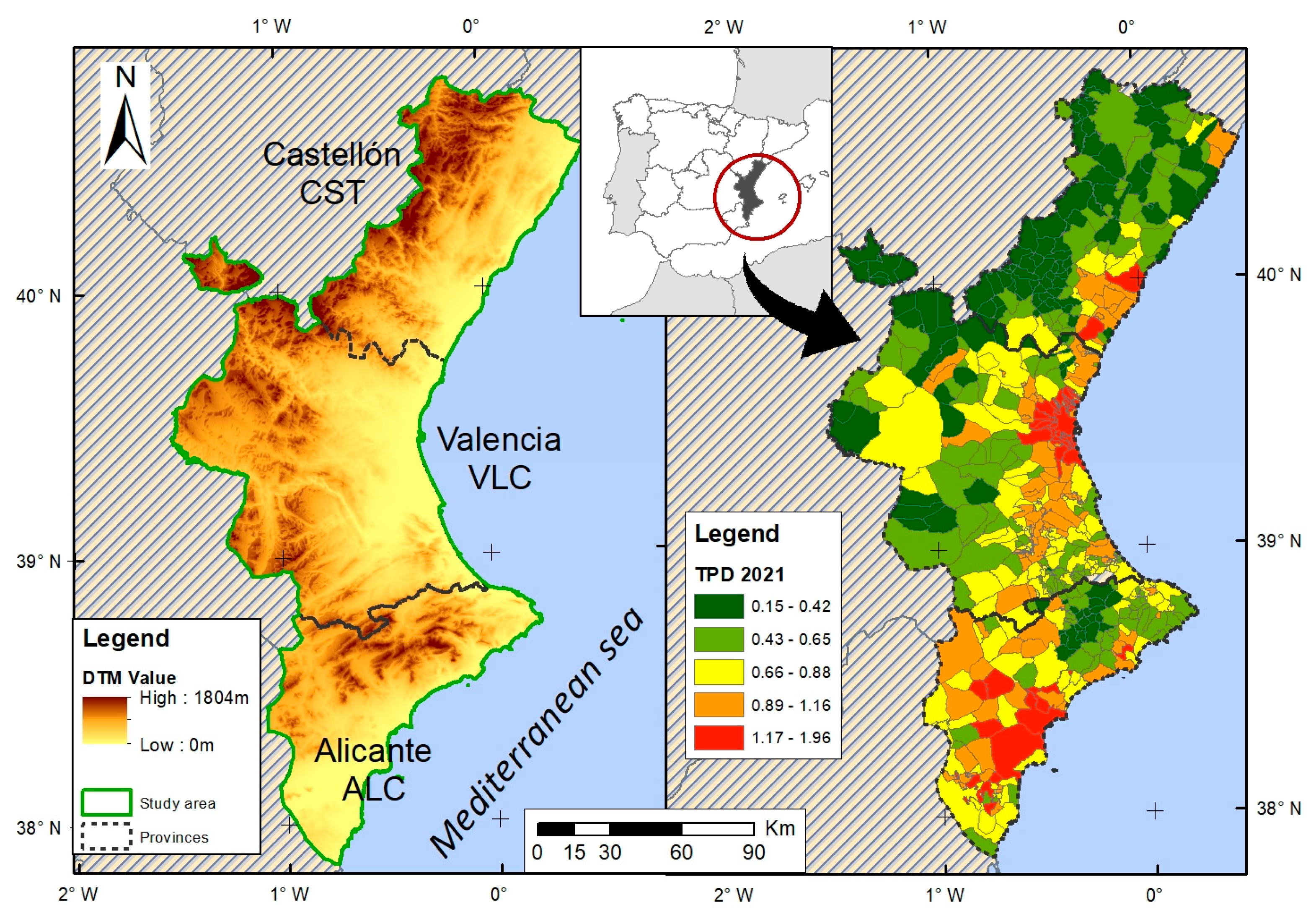
3.1.1. Susceptibility Mapping

The calculation of the danger level was based on the landslide susceptibility map (LSM) developed in a previous study [48,49]. Its characteristics are 25 × 25 m pixels as the surface area unit and spatial multi-criteria evaluation (SCME) to weight the factors to obtain the susceptibility values. The three significant factors used were slope, lithology, and land cover.

The susceptibility class thresholds defined in the above-mentioned previous study were used, obtained by means of an objective and thorough classification based on a Receiver Operating Characterisation (ROC) analysis, which uses the intrinsic variability of the data. From this map, the three highest susceptibility levels (Landslide Susceptibility Index, LSI) were selected to calculate the affected cadastral areas. These were LSI3 or L3 (medium), LSI4 or L4 (high), and LSI5 or L5 (very high).

3.1.2. Population

The Spanish National Statistics Institute (INE) is the official body that provides population data but it does not have complete data for series prior to 1981. This body offers very complete data from 1981 onwards and every 10 years thereafter, since that is when there are population censuses for the whole of Spain. But for previous years there is no geolocalised population data by municipality.

As a result, a series of raster distributions of population from outside of official bodies had to be resorted to. An example of the progress being made in this field on a global scale, through processes of downscaling the municipal population to the grid, is the Global Human Settlement Layer (GHSL) grid population data version R2023A [50], with a resolution of 1 km × 1 km, which provides results for 1975, 1980, 1990, 2000, 2010, and 2020. The GHSL is a worldwide product that had to be masked by Spain’s administrative boundaries; however, its resolution and temporal distribution is inadequate for the proposed objectives.

Fortunately, some very recent work is available that does fit this study’s approach. In [45], the author offers a grid with 100 × 100 m resolution and decennial periodicity between 1900 and 2021 (HIPGDAC-ES), which is based on previous studies by the author and on the extensive disaggregation of the Spanish Cadastre by [51]. Population was allocated to each cell by applying dasymetric techniques based on the data provided in the above-mentioned publications.

This population grid avoids population dispersion and agglomerates it in the most populated areas unlike the GHSL which disperses the population more widely, and with a much larger cell size. GHSL uses raster layers of built-up areas derived from satellite imagery, categorised according to their functional classification (residential versus non-residential) and incorporating an estimate of the building as a volume obtained by building height. The Goerlich method favours aggregation over dispersion, so many possible second homes in isolated areas are not assigned population. In contrast, GHSL offers many more inhabited cells than HIPGDAC-ES.

The concentration of the population offered by HIPGDAC-ES is useful for studies on landslides, for instance, which generally occur in peri-urban areas and which would otherwise overestimate the population affected by landslides, noting that many of them can occur at second homes.

3.1.3. Cadastre

The cadastral plot data were obtained from the Cadastral Mapping Services according to Inspire offered by the General Directorate of the Cadastre. The cadastral information adapted to the European directive Inspire is offered through interoperable services (WMS and WFS) and downloaded by municipality.

There are fields within this information necessary for this paper, such as the built-up area (GFA), the year of construction, and the type of use. The functional and residential cadastral plots have been selected, removing all those whose construction date was prior to 1800 for the initial calculation.

This date filter serves as a starting point, and has been considered adequate as a reference to start processing the cadastral information and to perform the cumulative calculation of the built-up area. Logically, it should be noted that there are few buildings dating from before 1800, especially in thinly populated municipalities. The filter in place disregards areas with limited residential buildings.

It has been observed that many cadastral plots in small towns were not registered until 1910 or 1920 even though they are older. This results in very high yet unrepresentative population density values at the beginning of the century, which has made it advisable to disregard those decades and start the calculations in 1920.

3.2. Method Implementation

As indicated in the methodology section (see Figure 1), this study seeks to locate the municipalities in which part of the population is in an area at risk of landslides. The goal is to calculate the distribution of this population within the municipality, together with the rate of area affected with respect to the total and its variation over time. For this purpose, the indices described in Section 2 will be used.

An extensive period of reference decades has been selected, as extensive series of cadastral and population data are available. In this period, the 1960s–70s and 1970s–80s stand out as the point of economic growth and the beginning of tourism, as well as 2011 (end of the real estate bubble) and 2021 (the year of the pandemic). As indicated above, the starting point was taken as the year 1800 (origin “0”, previously with no risk and no computable buildings) and the two initial decades were disregarded, the first period being 1800–1920 and the second 1920–1930, already with growth values. The following are calendar decades until 2021. From 1981 onwards, the beginning of each decade coincides with the population census carried out every 10 years by the National Statistics Institute.

The long period analysed allows the evolution of the built-up areas and those at risk to be studied by examining the evolution of the growth curve and finding its singular points. It also shows the affected population according to its location between the medium and very high susceptibility levels of the LSM mapping.

The key strength of this study is that the same procedure was carried out for the large area occupied by the Valencian Community, and the results obtained were perfectly comparable, although the calculation does at times present some uncertainty associated in particular with the resolution of the population grid used.

3.2.1. Calculation of Affected Population

This calculation is based on the aforementioned 100 × 100 m HIPGDAC-ES decennial population grid for the whole of Spain and the 25 × 25 m LSM maps for each province. The procedure applied (see Figure 4) is to determine the population at the highest susceptibility levels and then to count it for each municipality. As a first step, a raster with the same resolution and datum (100 × 100 m and LAEA) was created for the three provinces as a whole with exact cartographic adjustments.

Then the cells of the LSM raster that have a value that represents the joint value of the original cells were selected. They can be grouped into various levels of susceptibility. The affected population will be considered to be populations in the medium to very high levels, or levels 3 to 5. Therefore, the mean of the resulting cell will exactly match the value 3 or higher obtained by the LSM.

All calculations of built-up area, equivalent LSM, and affected population were carried out using scripts programmed in Python 2.7 with the geoprocessor provided by ESRI’s ArcGIS. As a result, all these data are offered for the 542 municipalities in the Valencian Community, using the same calculation procedure, which can be consulted as an appendix at the end of the article.

With this approach, 361 out of a total of 542 municipalities were identified as having some kind of impact on their population in 2021. It seems a conservative result, on the safe side, as it would represent almost 71,000 affected inhabitants, or 1.5% of the almost five million total inhabitants. To mitigate some inaccuracies in the method caused by the geolocation’s resolution, 78 municipalities with a population of under 10 inhabitants were removed as non-computable residual risk. In short, 283 municipalities were considered to be at significant risk in 2021, and 239 in 1960, in both cases more than half of the Valencian Community’s total. Obviously, it cannot be considered an imminent risk for the population in these municipalities, but the results conclude that there is a group in which the risk and its prognosis are concentrated, and these are the places where the necessary prevention and surveillance should be prioritised.

Special attention has been paid to the dates cadastral plots were registered at the beginning of the last century. Indeed, it has been observed that in quite a number of smaller municipalities there is a notable lack of registered residential area, resulting in excessively high population densities. As shown in the results section, the initial series had to be shortened to avoid the appearance of anomalous data caused by this circumstance.

It is, it should be noted, also difficult to differentiate between second homes and permanent dwellings for the purposes of allocating population. Although this is a problem that cannot be resolved by this study, it has been observed that the population grid does in many cases respect these holiday areas. Indeed, it has been shown that many municipalities may have built-up areas at risk and yet have no population affected. Therefore, the population is not distributed strictly dasymetrically, and the distribution routines, when rounding the population, partially disregard those second homes located on the periphery of the town centre.

3.2.2. Obtaining Indices

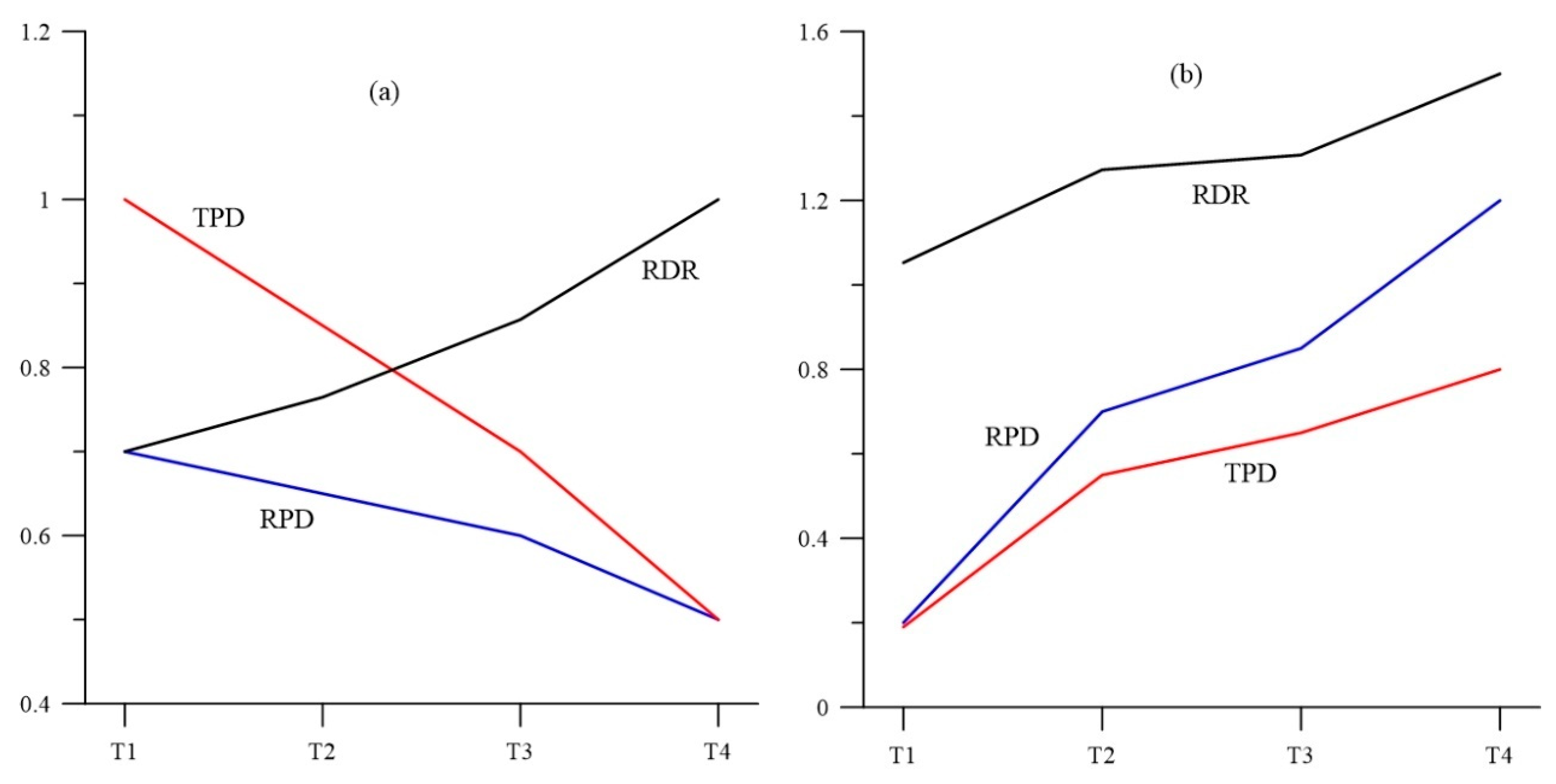
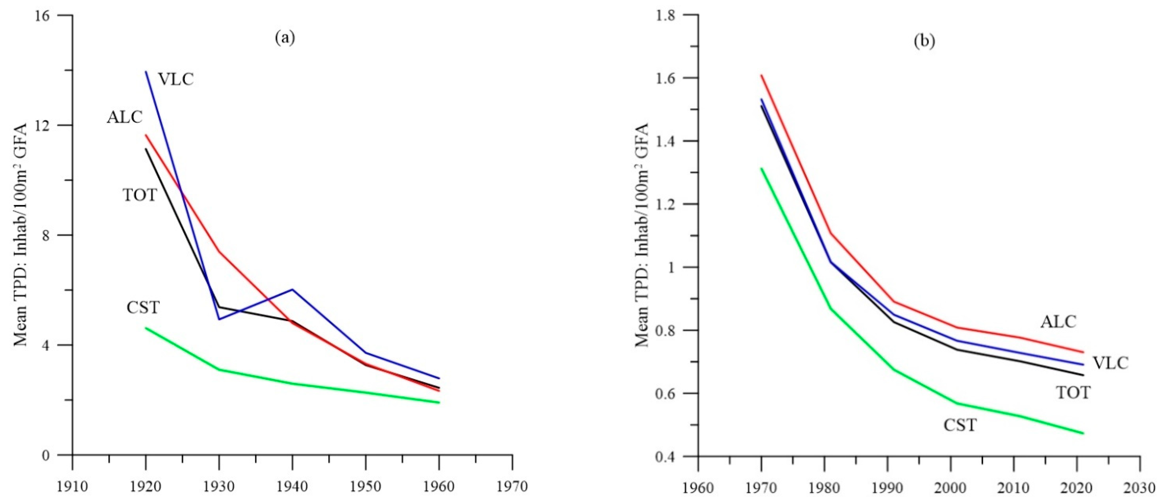
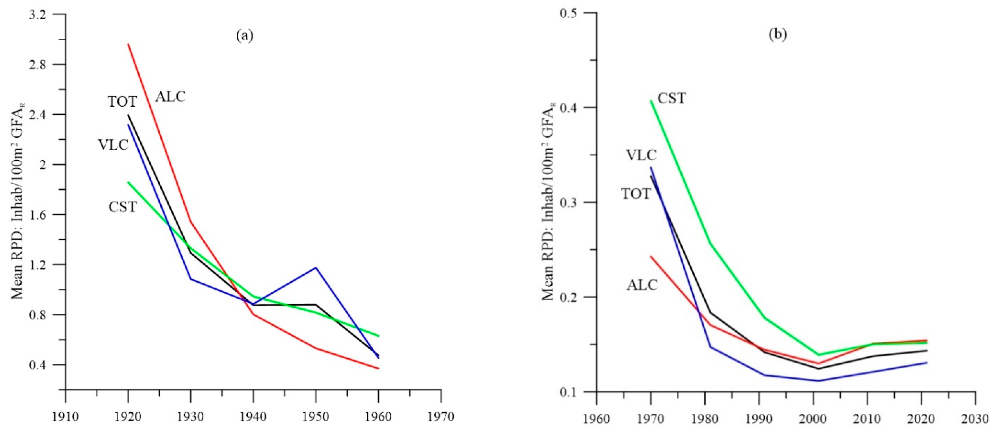
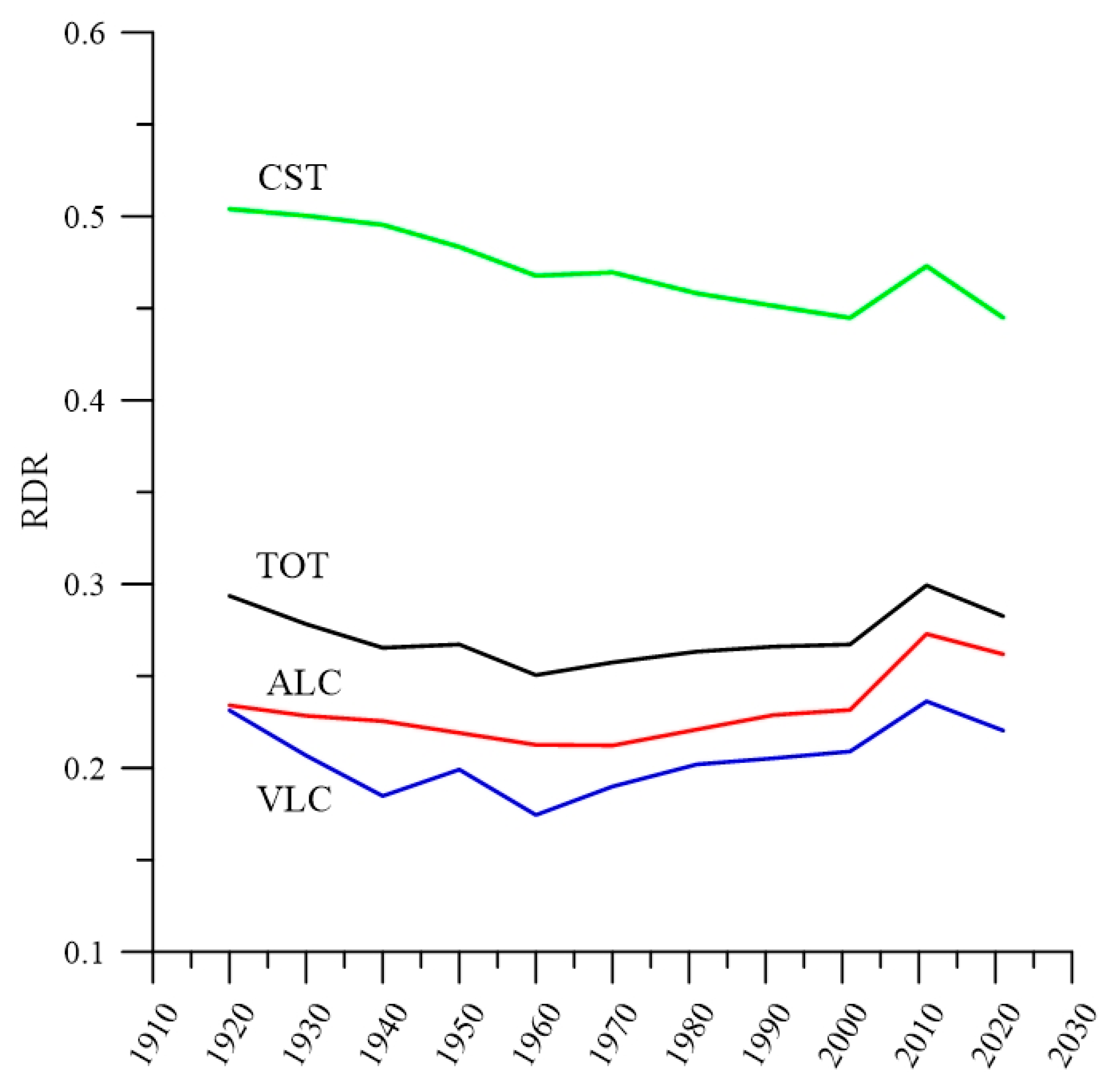
Section 2 details a number of indices suitable for parameterising risk in a given area. The dimensionless status indices are RSR, RPR, and RPD, and the calculation of population densities is also included as TPD and RPD. The dynamic index mRDR is shown to be highly explanatory for determining the trend of the population affected by landslide risk in the time series considered.

The first step was to differentiate between two working periods because of the long time series and thus to be able to distinguish behaviours. A first period, known as the historical period, was defined as between 1920 and 1960, just at the limit of the demographic and tourism boom that began in 1970 and that marks an important turning point. For the current, “recent” period, the series is defined as 1970 to 2021 (the latter years coinciding with the censuses), which better reflects the current trend.

The status indices (RSR, RPR, RDR, TPD, and RPD) were calculated for the end of the two periods originally considered, i.e., 1960 and 2021. The historical and recent periods were considered to calculate mRDR, and calculated in sexagesimal degrees.

4. Results

All available data were analysed according to the methodology proposed and are summarised in the graphs below. Of particular interest are the data on the evolution of population and built-up area, both restricted to the 239 (historical series) or 283 (recent) municipalities with significant risk (Figure 5). The term “net (n)” refers to the built-up area or population directly affected by the potential for landslides; the term “total (t)” is the overall area of a UAD affected in whole or in part.

Firstly, the evolution of the built-up area is clearly marked by the country’s demographic and economic growth, as well as the beginning of tourism from 1960–70 onwards. The years 1981–2021 were chosen to calculate the trend of the recent period as the previous period of intense growth should be excluded.

The increases in both the overall area and the area at risk are quite similar. However, there are clearly different behaviours by province. In the province of Alicante, the surface area under risk increases more than the overall surface area, while in the other two provinces, construction outside the risk zone is predominant. This seems to be caused by the increased urban pressure on the province as an internationally recognised tourist destination along the coastline. Figure 6 shows the major increase in population at risk in the province of Alicante compared to the stability of Castellón.

Figure 7 offers very significant data regarding the province of Alicante’s different behaviour from Castellón’s. The drop in population affected right up to the start of the tourism boom in the 1960s is of note. It points to a certain depopulation coupled with non-expansive construction in at-risk areas. Alicante shows a notable increase as it is the most benefited by tourism. Castellón, on the other hand, tends to fall as it is not as marked a tourist and holiday destination as Alicante.

The graphs of Figure 8 highlight the high average population density in the at-risk zone at the beginning of the historical period. This can only be explained if the lack of built surface area in the first decades due to the aforementioned problem with cadastral dates is taken into account, a phenomenon which was more accentuated in the provinces of Castellón and Alicante. This situation fully justifies reducing the historical period to the 1920–1960 series. The decline in average density in the recent series is mainly due to a decline in population in the areas concerned which is not accompanied by a significant increase in built-up area. This is even more evident in the graph for the province of Castellón. The curve stabilises with a slight upward trend from 2001 onwards.

The maps in Figure 9 confirm all the indications in the previous graphs. The decrease in the affected population in the province of Castellón is notable, caused by the depopulation of inland villages, while it increases in Alicante, mainly due to the effect of tourism and second homes along the coast.

The slight trend observed in the historical series corresponds to the situation expressed in Figure 2 but conversely: TPD decreases more than RPD (see Figure 7a and Figure 8a). This indicates a slight tendency for residential construction to avoid risky areas. In the recent series, the slight increase in RDR is due, as can be seen in Figure 7b and Figure 8b, to a change in trend, with construction occupying at-risk zones (see Figure 2). There is a high RDR value for the province of Castellón (Figure 10), indicating a higher concentration of risk, largely as a result of including municipalities with smaller populations than the other provinces. Small municipalities have higher RDR values and also keep this value stable for a longer period of time throughout the historical series due to less construction and population dynamics. Finally, the small variation in RDR values across the series indicates a general continuity or stability of the risk situation.

In the early period before 1900 and in the 1900–10 decade, some RSR values > 1.0 (even significantly higher) appear in some municipalities, decreasing afterwards towards normal values. This confirms that in these cases the dates of the cadastral data need to be reviewed and are not entirely reliable. All this confirms the decision taken to exclude this period to exclude Cadastre inaccuracies, selecting the series between 1920 and 1960 to calculate mRDR60.

Table 2. Means of variables and population totals for historical series.

	RPD60	RSR60	RPR60	RDR60	mRDR60	PopT60	PopR60
Total	0.62	0.33	0.13	0.25	−1.39	924,004	47,715
ALC	0.47	0.28	0.09	0.21	−1.46	370,738	17,706
CST	0.87	0.49	0.28	0.47	−1.73	158,473	15,741
VLC	0.62	0.28	0.08	0.17	−1.17	394,793	14,268

and

Table 3. Means of variables and population totals for recent series.

	RPD21	RSR21	RPR21	RDR21	mRDR21	PopT21	PopR21
Total	0.16	0.34	0.13	0.29	3.71	2,416,466	62,499
ALC	0.17	0.32	0.11	0.27	6.44	1,129,943	39,410
CST	0.19	0.49	0.28	0.46	−0.23	319,097	7700
VLC	0.14	0.29	0.08	0.23	3.53	967,426	15,389

below show the averages of the defined variables and the sum of populations for the two series: historical (239 municipalities) and recent (283).

The tables above highlight the decreasing value of mRDR in the historical series, due to depopulation and lack of continued construction. The fact that the province of Castellón has less population at risk recently than historically is also of note, a finding explained by the higher incidence of risk in inland towns that have not undergone recent urban expansion, whereas in Alicante the opposite is true.

5. Discussion

With the data processed, it is important to observe how the municipalities studied are organised and what type of association there may be between them, according to the status and trend indicators calculated. To do so, a cluster analysis was run to determine the types of groupings that can be found in the area being studied. This type of analysis is a tool that has amply proven its usefulness in grouping urban areas by means of indicators [52,53,54].

5.1. Correlated Variables

In a cluster analysis, when distance is used as a similarity criterion, one should avoid using highly correlated variables because they include redundant information (principle of parsimony). A prior correlation analysis was run to select those variables most suitable for describing the groups. The criterion was to prioritise the degree of correlation in the recent period and with the variables that should better organise the groups. MRDR and those relating to population stand out due to their low correlation with the rest of the variables.

To avoid adding complexity to

Table 4. Correlation matrix. In bold, those referred to in the text.

.	RPD60	RPD 21	RSR 60	RSR 21	RPR 60	RPR 21	RDR 60	RDR 21	mRDR 60	mRDR 21	popR 60	popR 21	popT 60	popT 21
RPD60	1.00
RPD21	0.24	1.00
RSR60	0.06	0.13	1.00
RSR21	0.01	0.13	0.94	1.00
RPR60	0.14	0.39	0.80	0.76	1.00
RPR21	0.10	0.43	0.75	0.80	0.94	1.00
RDR60	0.27	0.42	0.57	0.51	0.83	0.75	1.00
RDR21	0.22	0.72	0.50	0.54	0.78	0.83	0.78	1.00
mRDR 60	0.01	0.02	0.10	0.08	0.08	0.06	−0.02	0.00	1.00
mRDR 21	−0.16	0.24	−0.13	0.02	−0.15	0.05	−0.30	0.14	−0.03	1.00
popR60	0.10	0.26	0.45	0.35	0.48	0.39	0.46	0.34	0.03	−0.21	1.00
popR21	−0.02	0.27	0.00	0.02	−0.01	0.04	−0.03	0.08	0.02	0.23	0.33	1.00
popT60	0.03	0.00	−0.20	−0.26	−0.16	−0.19	−0.04	−0.19	0.11	−0.13	0.31	0.28	1.00
popT21	0.00	−0.06	−0.33	−0.37	−0.24	−0.25	−0.16	−0.29	0.12	−0.08	0.07	0.32	0.76	1.00

, p-values indicating significant correlations when greater than 0.05 have not been included. In general, high correlation values (above approx. 0.20) are 95% statistically significant.

Table 4 shows that the only noteworthy mRDR value is with the at-risk population (0.23). Afterwards, high correlation values are observed for the rest of the variables and between the historical and recent series in general, which seems to confirm the continuity or stability observed in Figure 10. The RDR value is highly correlated to RPD (0.72), RPR (0.83), and RSR (0.54), as expected, the latter index being the least correlated and most interesting as an indicator of magnitude. RSR, RDR, mRDR, and popT were chosen as explanatory variables for the cluster analysis, excluding the rest of the variables due to their correlation. The municipal population was also included as a variable to indicate the importance of the municipality in absolute value. It should be noted that the total population is significantly correlated to the risk indicators, but with a negative sign, i.e., municipalities with larger populations have lower risk values; however, there is a positive correlation between the total population and the population at risk (0.32).

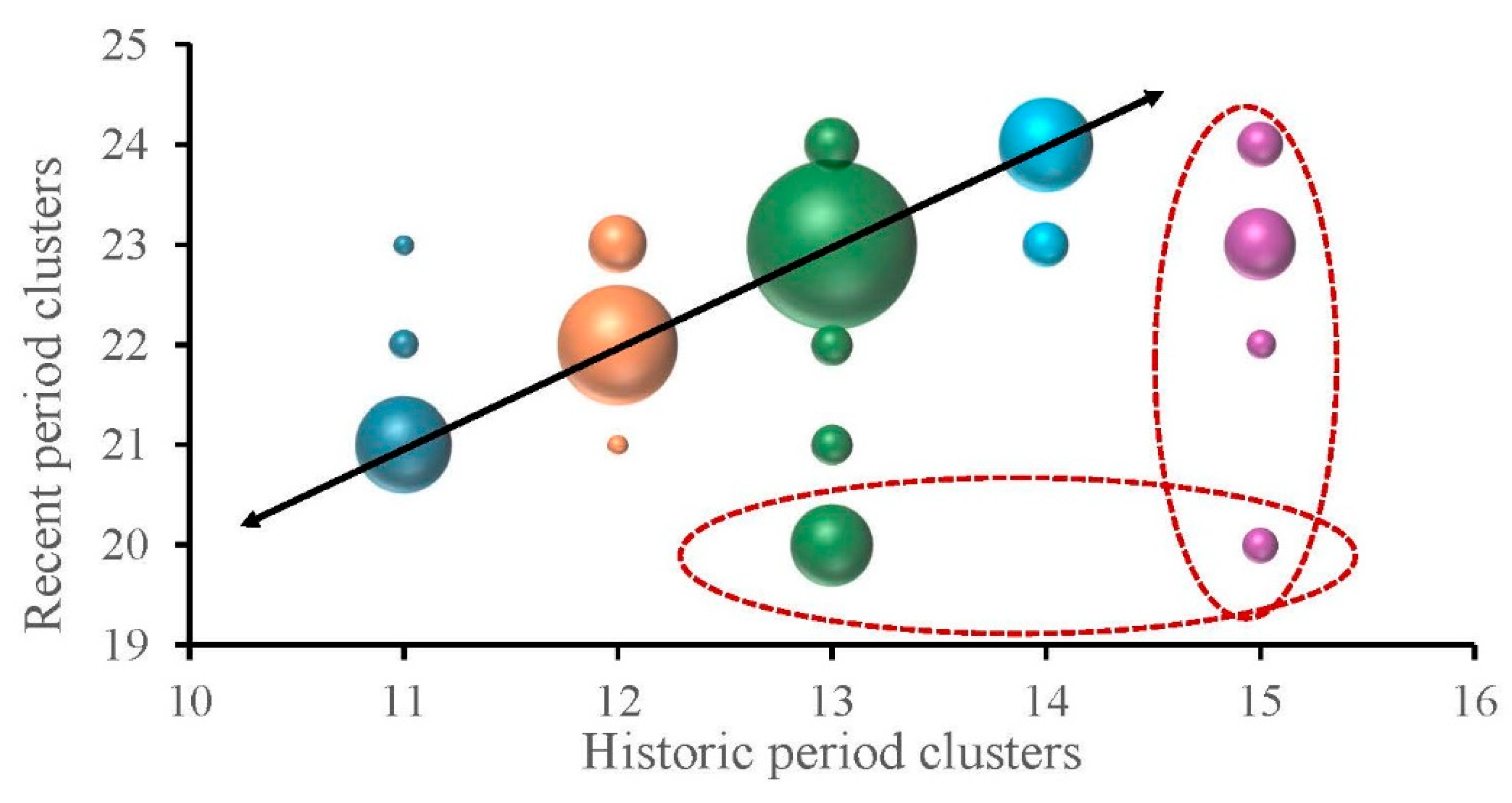
5.2. Cluster Analysis

The Ward method was chosen for the clustering method, applying the Euclidean distance. This method is considered the most appropriate since the information lost from merging elements is less than with others [55,56]. Moreover, this method is not very sensitive to outliers or extreme individuals and tends to form more compact clusters with similar sizes, which is an advantage when studying the behaviour of these groups of municipalities.

According to the correlation matrix, the variables RSR, RDR, mRDR, and popT were selected for the two time periods defined: historical and recent. However, the population value is classically distributed according to a “heavy tail” variable and greatly alters the outcome of the analysis. Indeed, the cluster analysis is very sensitive to extreme values, which is why the three cities with a population of over 200,000 inhabitants in the two series (Valencia, Alicante, Elche) were left out.

Table 5. Comparison of centroid clusters historical (HP) and recent (RP) period.

HP/RPCluster	N° UAD HP/RP	RDR 60	RDR 21	mRDR 60	mRDR 21	RSR 60	RSR 21	PopT 60	PopT 21
- -/c20	- -/43	- -	0.34	--	25.4	- -	0.25	- - -	4345
c11/c21	25/27	0.76	0.78	1.2	3.0	0.96	0.88	756	409
c12/c22	43/42	0.31	0.33	2.1	−0.4	0.73	0.70	1491	881
c13/c23	118/124	0.26	0.20	4.2	−1.7	0.23	0.22	5384	3943
c14/c24	27/44	0.18	0.16	4.1	1.9	0.12	0.10	19,964	38,467
c15/- -	26/- -	0.35	- -	−42.6	- -	0.18	- -	2583	- - -

shows the result of the centroids of the five clusters that were determined as the minimum number to adequately describe the comparison between the two series addressed. Two different analyses were carried out for each series, using the 215 municipalities that meet all the conditions in each case, where all the variables initially used appear. It was found that four of the five clusters have similar centroids in both series, which proves the line of continuity throughout the whole period studied.

Table 6. Cluster characteristics historical (ClsHP) and recent period (ClsRP).

ClsHP	ClsRP	Values	Description
--	c20	High mRDR21	Municipalities with a significant increase in RDR, over-occupation of low-risk areas. The area at risk also increases.
c11	c21	High RSR High RDR Low population	Very small municipalities located in inland areas, directly affecting the town centre. Higher than average risk. Declining population in the recent series.
c12	c22	High RSR Medium RDR Low population	Small municipalities. The risk area does not directly or only partially affects the downtown of the most populated town centre. Sharp decline in population.
c13	c23	Average	Numerous groups of municipalities with medium risk without noteworthy values.
c14	c24	High population Low RDR Low RSR	Large municipalities. The population is increasing in the recent series, but its RDR is low due to low occupancy in the risk zone.
c15	--	Low mRDR60 Low RSR	Municipalities with medium population. Decreasing risk trend as construction in affected areas decreases.

shows the important reference values to make the groupings, leaving two very representative clusters unpaired. Firstly, the time series cluster that groups together municipalities with a clear decrease in the RDR value (c15). And then, in the recent series, a cluster with the opposite characteristics: municipalities with a marked increase in the value of RDR (c20). Table 6 shows the characteristics of each cluster along with their pairing.

These results show how the clusters of the two periods addressed are distributed, encompassing a total of 215 municipalities, which are the ones that have all the data for both periods.

In Figure 11, a 3D bubble chart shows the distribution of municipalities per cluster, the number of which is proportional to the size of the sphere. The ovals show the municipalities with differential development. In general, the evolution of risk is natural according to the clusters obtained, from c11 to c21, c12 to c22, …, located on the main diagonal, which indicates that there were no major changes in this set of 145 municipalities for a century (almost 70% of the municipalities with significant risk). It should be noted that three municipalities in Alicante evolve from c15 to c20, and 16 municipalities from c13 to c20; the rest of the 23 municipalities in c20 had no significant history of risk in the historical period.

Of the 43 municipalities with increasing risk (c20), Millares is notable for its unique location in a mountainous inland area and its small population. The rest are either on the coastal strip or close to large cities or major roads. Millares shows a marked decrease in the RDR in the 1980s, as more than 50% of the residential building in the recent period was registered in that decade (major economic activity due to the location of a short-lived textile factory in the 80s–90s), causing this decrease which results in a slope value that cannot be extrapolated.

Figure 12 shows two maps with the geolocation by municipality of all the clusters in the two periods. The concentration of cluster 20 along the coast of Alicante should be noted. This is the La Marina region, an area that has already been studied by the same authors [57] and whose results do not differ from those presented in this paper. This study, please note, was carried out by considering only the evolution of the risk assessed in economic units, without including in any way the population affected.

The result of the cluster analysis was very revealing as it established groups of municipalities in a large area that have common characteristics both in terms of their situation and their evolution. It is particularly relevant that in four of the five groups established, the characteristics of the historical series are maintained in the recent series.

One of the remaining groups is notable for bringing together dozens of municipalities that show an upward trend in risk, presumably due to their population dynamics and tourism and holiday activity. Indeed, many of them are located on the coastal strip, where areas of high residential value are located. According to the above, construction expansion may lead to the occupation of risk areas given the lack of conventional land and the need to meet demand, often at high prices.

This is the case of well-known coastal towns in the province of Alicante with a large amount of tourism, although not all of them present the aforementioned increased risk. Factors such as building pressure in certain coastal areas lead to rising demand and consequent increases in land value, making it difficult to access land that is without any risk. Or even often not avoiding the risk because the desire for scenic locations or areas closer to the coastline is so great. This problem has already been noted [57].

At the other extreme is the province of Castellón, with very few towns at high risk. This is due to a much smaller demographic dynamic, with inland locations, poor connections, and less building pressure. It is also relevant that the coastal strip, which is also mountainous and of great tourism value, has such a different value when compared with the province of Alicante. It should be noted that a large part of this coastal mountainous strip was declared a regional natural park, which means there are major limits on construction that indirectly allow the population to avoid the risk of landslides.

The province of Valencia, to conclude, has no mountains along its coastline, with the exception of a single municipality which, however, is not affected in a major way by the risk of landslides (cluster C24). The Valencian municipalities at most risk are located in mountainous interior regions and close to the main roads.

6. Conclusions

In this study, the increase in risk is mainly due to inappropriate locations of risk-prone elements, i.e., those subject to more exposure. In terms of residential building, this occurs when construction takes place in areas at risk, due to housing or holiday pressure in tourism areas.

To determine risk growth characteristics and trends, in this study a series of indices were defined, which are easy to obtain and replicable in any study of this kind. The RDR index has proven to be particularly useful as a dimensionless descriptor of risk and one that adequately characterises municipalities’ risk situation. Its analysis in time series has made it possible to find out its evolution, a fundamental aspect to determine the effectiveness of each municipality’s territorial management.

As a result, a certain stability in the evolution of risk has been observed due to the fact that construction tends to be mainly built in non-risk areas. This fact is clearly evident in the historical series, a result that can be considered expected, as it is an attenuated expansion that is exclusively a product of the need for housing. In the recent period, many municipalities maintain this line of stability (67% of municipalities with significant risk). However, some of them radically change their tendency to accommodate holiday homes whose pace of construction and location requirements force them to locate new buildings in risk areas.

Indeed, there are a number of municipalities identified in this paper whose spatial planners should be more vigilant. They should do so by applying greater control on areas where urban development extends into mountainous areas. These areas are highlighted in Figure 12 and are mostly located in the region of La Marina, in the north of the province of Alicante. These municipalities are close to the coast, receive high-income tourists, and have limited possibilities for urban expansion. The new constructions end up occupying land with a higher risk of landslides, among other problems that are not inconsequential in nature (environmental, infrastructural, etc.).

These conclusions are not definitive, as the resolution of the population data needs to be improved to obtain more detailed and conclusive results. The problem of the cadastral estates at the beginning of the last century is not relevant, especially when during the first half of the century the risk was stable and allocated to inland municipalities. In terms of resolution improvement, grids of 50 × 50 m, or, even better, 25 × 25 m or 10 × 10 m, would be required. Advances in high detail mapping information may lead to such maps using dasymetric techniques. The major problem lies in cataloguing second homes and being able to allocate inhabitants accordingly. Therefore, bearing in mind that these second homes tend to occupy land at risk, it may be erring on the side of excess to allocate population to second homes at risk that are actually unoccupied for a large part of the year.

It should be noted that the limitations of the method are mainly determined by the availability of the data used to apply it in other contexts. In addition to the susceptibility map, geolocated data on population and residential housing with adequate resolution (at least 100 × 100 m) are required. While such data are available for the entire Spanish territory, as previously mentioned, their availability may be more limited in other countries. Nevertheless, current trends in national Spatial Data Infrastructures are moving in this direction.

This study sets out a series of guidelines together with easily obtainable indicators to determine the status and development of risk. It should be noted that studies that analyse the evolution of risk in the population in long series are uncommon, and this study has allowed us to understand the behaviour of risk in previous historical series. The above findings confirm the need to study the evolution of risk over extended periods of time.

This is a pioneering inquiry that needs to be improved and extended, but it is a necessary starting point in the dynamic study of landslide risk in mountainous areas, especially those with a certain degree of interest as a holiday destination. These results therefore need to be tested and validated in other settings and with more precise data, and risk data with an economic value incorporated and combined with risk to the population to gain a complete scenario that can better meet the challenge of risk prevention.

Finally, estimating the number of affected inhabitants per municipality and their prognosis is considered essential to establish objective territorial planning procedures and to increase the resilience of the social fabric, as well as to increase the efficiency of the monitoring plans and emergency actions put in place by civil protection agencies. Indeed, by taking into account the potentially affected inhabitants, prioritisation of the identified areas will improve the accuracy of rescue operations. In light of recent disasters, some of them close to home, all protocols aimed at reducing damage to buildings and infrastructures and, of course, saving lives, should be fostered.

References

1. Chen, C.W.; Tung, Y.S.; Chu, F.Y.; Li, H.C.; Chen, Y.M. Assessing landslide risks across varied land-use types in the face of climate change. Landslides 2024, 1–15. [Google Scholar] [CrossRef]
2. Gariano, S.L.; Guzzetti, F. Landslides in a changing climate. Earth-Sci. Rev. 2016, 162, 227–252. [Google Scholar] [CrossRef]
3. Haque, U.; Da Silva, P.F.; Devoli, G.; Pilz, J.; Zhao, B.; Khaloua, A.; Wilopo, W.; Andersen, P.; Lu, P.; Lee, J.; et al. The human cost of global warming: Deadly landslides and their triggers (1995–2014). Sci. Total Environ. 2019, 682, 673–684. [Google Scholar] [CrossRef]
4. Moore, R.; McInnes, R. The impacts of landslides on global society: Planning for change. Landslides Eng. Slopes. Exp. Theory Pract. 2016, 3, 1461–1468. [Google Scholar] [CrossRef]
5. Fuchs, S. Susceptibility versus resilience to mountain hazards in Austria—Paradigms of vulnerability revisited. Nat. Hazards Earth Syst. Sci. 2009, 9, 337–352. [Google Scholar] [CrossRef]
6. Kienberger, S.; Lang, S.; Zeil, P. Spatial vulnerability units—Expert-based spatial modelling of socio-economic vulnerability in the Salzach catchment, Austria. Nat. Hazards Earth Syst. Sci. 2009, 9, 767–778. [Google Scholar] [CrossRef]
7. Papathoma-Köhle, M.; Kappes, M.; Keiler, M.; Glade, T. Physical vulnerability assessment for alpine hazards: State of the art and future needs. Nat. Hazards J. Int. Soc. Prev. Mitig. Nat. Hazards 2011, 58, 645–680. [Google Scholar] [CrossRef]
8. Kappes, M.S.; Papathoma-Köhle, M.; Keiler, M. Assessing physical vulnerability for multi-hazards using an indicator-based methodology. Appl. Geogr. 2012, 32, 577–590. [Google Scholar] [CrossRef]
9. Fuchs, S.; Kuhlicke, C.; Meyer, V. Editorial for the special issue: Vulnerability to natural hazards-the challenge of integration. Nat. Hazards 2011, 58, 609–619. [Google Scholar] [CrossRef]
10. Karagiorgos, K.; Thaler, T.; Hübl, J.; Maris, F.; Fuchs, S. Multi-vulnerability analysis for flash flood risk management. Nat. Hazards 2016, 82, 63–87. [Google Scholar] [CrossRef]
11. Michael-Leiba, M.; Baynes, F.; Scott, G.; Granger, K. Regional landslide risk to the Cairns community. Nat. Hazards 2003, 302, 233–249. [Google Scholar] [CrossRef]
12. Keiler, M. Development of the damage potential resulting from avalanche risk in the period 1950-2000, case study Galtür. Nat. Hazards Earth Syst. Sci. 2004, 4, 249–256. [Google Scholar] [CrossRef]
13. Promper, C.; Glade, T. Multilayer-exposure maps as a basis for a regional vulnerability assessment for landslides: Applied in Waidhofen/Ybbs, Austria. Nat. Hazards 2016, 82, 111–127. [Google Scholar] [CrossRef]
14. Fuchs, S.; Keiler, M.; Zischg, A. A spatiotemporal multi-hazard exposure assessment based on property data. Nat. Hazards Earth Syst. Sci. 2015, 15, 2127–2142. [Google Scholar] [CrossRef]
15. Guillard-Goncalves, C.; Zezere, J.L.; Pereira, S.; Garcia, R.A.C. Assessment of physical vulnerability of buildings and analysis of landslide risk at the municipal scale: Application to the Loures municipality, Portugal. Nat. Hazards Earth Syst. Sci. 2016, 16, 311–331. [Google Scholar] [CrossRef]
16. Petrucci, O.; Gullà, G. A simplified method for assessing landslide damage indices. Nat. Hazards J. Int. Soc. Prev. Mitig. Nat. Hazards 2010, 52, 539–560. [Google Scholar] [CrossRef]
17. Promper, C.; Gassner, C.; Glade, T. Spatiotemporal patterns of landslide exposure—A step within future landslide risk analysis on a regional scale applied in Waidhofen/Ybbs Austria. Int. J. Disaster Risk Reduct. 2015, 12, 25–33. [Google Scholar] [CrossRef]
18. Silva, M.; Pereira, S. Assessment of physical vulnerability and potential losses of buildings due to shallow slides. Nat. Hazards 2014, 72, 1029–1050. [Google Scholar] [CrossRef]
19. Uzielli, M.; Catani, F.; Tofani, V.; Casagli, N. Risk analysis for the Ancona landslide—II: Estimation of risk to buildings. Landslides 2015, 12, 83–100. [Google Scholar] [CrossRef]
20. Uzielli, M.; Catani, F.; Tofani, V.; Casagli, N. Risk analysis for the Ancona landslide—I: Characterization of landslide kinematics. Landslides 2015, 12, 69–82. [Google Scholar] [CrossRef]
21. Winter, M.G.; Smith, J.T.; Fotopoulou, S.; Pitilakis, K.; Mavrouli, O.; Corominas, J.; Argyroudis, S. An expert judgement approach to determining the physical vulnerability of roads to debris flow. Bull. Eng. Geol. Environ. 2014, 73, 291–305. [Google Scholar] [CrossRef]
22. De Oliveira Mendes, J.M. Social vulnerability indexes as planning tools: Beyond the preparedness paradigm. J. Risk Res. 2009, 12, 43–58. [Google Scholar] [CrossRef]
23. Wood, N.J.; Burton, C.G.; Cutter, S.L. Community variations in social vulnerability to Cascadia-related tsunamis in the U.S. Pacific Northwest. Nat. Hazards J. Int. Soc. Prev. Mitig. Nat. Hazards 2010, 52, 369–389. [Google Scholar] [CrossRef]
24. Di Napoli, M.; Miele, P.; Guerriero, L.; Corona, M.A.; Calcaterra, D.; Ramondini, M.; Sellers, C.; Martire, D.D. Multitemporal relative landslide exposure and risk analysis for the sustainable development of rapidly growing cities. Landslides 2023, 20, 1781–1795. [Google Scholar] [CrossRef]
25. Bukhari, M.H.; da Silva, P.F.; Pilz, J.; Istanbulluoglu, E.; Görüm, T.; Lee, J.; Karamehic-Muratovic, A.; Urmi, T.; Soltani, A.; Wilopo, W.; et al. Community perceptions of landslide risk and susceptibility: A multi-country study. Landslides 2023, 20, 1321–1334. [Google Scholar] [CrossRef]
26. Guzzetti, F. Landslide fatalities and the evaluation of landslide risk in Italy. Eng. Geol. 2000, 58, 89–107. [Google Scholar] [CrossRef]
27. Vranken, L.; Van Turnhout, P.; Van Den Eeckhaut, M.; Vandekerckhove, L.; Poesen, J. Economic valuation of landslide damage in hilly regions: A case study from Flanders, Belgium. Sci. Total Environ. 2013, 447, 323–336. [Google Scholar] [CrossRef]
28. Fidan, S.; Tanyaş, H.; Akbaş, A.; Lombardo, L.; Petley, D.N.; Görüm, T. Understanding fatal landslides at global scales: A summary of topographic, climatic, and anthropogenic perspectives. Nat. Hazards 2024, 120, 6437–6455. [Google Scholar] [CrossRef]
29. Guzzetti, F.; Stark, C.P.; Salvati, P. Evaluation of flood and landslide risk to the population of Italy. Environ. Manag. 2005, 36, 15–36. [Google Scholar] [CrossRef]
30. Gariano, S.L.; Petrucci, O.; Guzzetti, F. Changes in the occurrence of rainfall-induced landslides in Calabria, southern Italy, in the 20th century. Nat. Hazards Earth Syst. Sci. 2015, 15, 2313–2330. [Google Scholar] [CrossRef]
31. Zêzere, J.L.; Oliveira, S.C.; Garcia, R.A.C.; Reis, E. Landslide risk analysis in the area North of Lisbon (Portugal): Evaluation of direct and indirect costs resulting from a motorway disruption by slope movements. Landslides 2007, 4, 123–136. [Google Scholar] [CrossRef]
32. Zêzere, J.L.; Garcia, R.A.C.; Oliveira, S.C.; Reis, E. Probabilistic landslide risk analysis considering direct costs in the area north of Lisbon (Portugal). Geomorphology 2008, 94, 467–495. [Google Scholar] [CrossRef]
33. Remondo, J.; Bonachea, J.; Cendrero, A. Quantitative landslide risk assessment and mapping on the basis of recent occurrences. Geomorphology 2008, 94, 496–507. [Google Scholar] [CrossRef]
34. Corominas, J.; Van Westen, C.; Frattini, P.; Cascini, L.; Malet, J.-P.; Fotopoulou, S.; Catani, F.; Van Den Eeckhaut, M.; Mavrouli, O.; Agliardi, F.; et al. Recommendations for the quantitative analysis of landslide risk. Bull. Eng. Geol. Environ. 2014, 73, 209–263. [Google Scholar] [CrossRef]
35. Schwendtner, B.; Papathoma-Köhle, M.; Glade, T. Risk evolution: How can changes in the built environment influence the potential loss of natural hazards? Nat. Hazards Earth Syst. Sci. 2013, 13, 2195–2207. [Google Scholar] [CrossRef]
36. Su, M.D.; Lin, M.C.; Hsieh, H.I.; Tsai, B.W.; Lin, C.H. Multi-layer multi-class dasymetric mapping to estimate population distribution. Sci. Total Environ. 2010, 408, 4807–4816. [Google Scholar] [CrossRef]
37. Freire, S.; Aubrecht, C. Integrating population dynamics into mapping human exposure to seismic hazard. Nat. Hazards Earth Syst. Sci. 2012, 12, 3533–3543. [Google Scholar] [CrossRef]
38. Aubrecht, C.; Özceylan, D.; Steinnocher, K.; Freire, S. Multi-level geospatial modeling of human exposure patterns and vulnerability indicators. Nat. Hazards 2013, 68, 147–163. [Google Scholar] [CrossRef]
39. Opdyke, A.; Fatima, K. Comparing the suitability of global gridded population datasets for local landslide risk assessments. Nat. Hazards 2024, 120, 2415–2432. [Google Scholar] [CrossRef]
40. Bhaduri, B.L.; Bright, E.A.; Dobson, J.E. LandScan: Locating People is What Matters. Geoinfomatics 2002, 5(2), 34–37. [Google Scholar]
41. Wen, H.; Huang, J.; Qian, L.; Li, Z.; Zhang, Y.; Zhang, J. The spatial-temporal evolution patterns of landslide-oriented resilience in mountainous city: A case study of Chongqing, China. J. Environ. Manag. 2024, 370, 122963. [Google Scholar] [CrossRef] [PubMed]
42. Meerow, S.; Newell, J.P.; Stults, M. Defining urban resilience: A review. Landsc. Urban Plan. 2016, 147, 38–49. [Google Scholar] [CrossRef]
43. Tian, N.; Lan, H. The indispensable role of resilience in rational landslide risk management for social sustainability. Geogr. Sustain. 2023, 4, 70–83. [Google Scholar] [CrossRef]
44. Garcia, R.A.C.; Oliveira, S.C.; Zêzere, J.L. Assessing population exposure for landslide risk analysis using dasymetric cartography. Nat. Hazards Earth Syst. Sci. 2016, 16, 2769–2782. [Google Scholar] [CrossRef]
45. Goerlich, F.J. HIPGDAC-ES: Historical population grid data compilation for Spain (1900–2021). Sci. Data 2025, 12, 280. [Google Scholar] [CrossRef]
46. Fell, R.; Corominas, J.; Bonnard, C.; Cascini, L.; Leroi, E.; Savage, W.Z. Guidelines for landslide susceptibility, hazard and risk zoning for land use planning. Eng. Geol. 2008, 102, 85–98. [Google Scholar] [CrossRef]
47. Günther, A.; Van Den Eeckhaut, M.; Malet, J.P.; Reichenbach, P.; Hervás, J. Climate-physiographically differentiated Pan-European landslide susceptibility assessment using spatial multi-criteria evaluation and transnational landslide information. Geomorphology 2014, 224, 69–85. [Google Scholar] [CrossRef]
48. Cantarino, I.; Carrion, M.A.; Goerlich, F.; Ibañez, V.M. A ROC analysis-based classification method for landslide susceptibility maps. Landslides 2019, 16, 265–282. [Google Scholar] [CrossRef]
49. Cantarino, M.; Carrion, A.; Martínez-Ibáñez, V.; Gielen, E. Improving Landslide Susceptibility Assessment through Frequency Ratio and Classification Methods—Case Study of Valencia Region (Spain). Appl. Sci. 2023, 13, 5146. [Google Scholar] [CrossRef]
50. European Commission. GHS-POP R2023A—GHS Population Grid Multitemporal. Joint Research Centre Data Catalogue. Available online: https://data.jrc.ec.europa.eu/dataset/2ff68a52-5b5b-4a22-8f40-c41da8332cfe (accessed on 12 March 2025).
51. Uhl, J.H.; Royé, D.; Burghardt, K.; Vázquez, J.A.A.; Sanchiz, M.B.; Leyk, S. HISDAC-ES: Historical settlement data compilation for Spain (1900–2020). Earth Syst. Sci. Data 2023, 15, 4713–4747. [Google Scholar] [CrossRef]
52. Huang, J.; Lu, X.X.; Sellers, J.M. A global comparative analysis of urban form: Applying spatial metrics and remote sensing. Landsc. Urban Plan. 2007, 82, 184–197. [Google Scholar] [CrossRef]
53. Stewart, T.J.; Janssen, R. A multiobjective GIS-based land use planning algorithm. Comput. Environ. Urban Syst. 2014, 46, 25–34. [Google Scholar] [CrossRef]
54. Gisbert, F.J.G.; Martí, I.C.; Gielen, E. Clustering cities through urban metrics analysis. J. Urban Des. 2017, 22, 689–708. [Google Scholar] [CrossRef]
55. Kuiper, F.K.; Fisher, L. 391: A Monte Carlo Comparison of Six Clustering Procedures. Biometrics 1975, 31, 777. [Google Scholar] [CrossRef]
56. Sarstedt, M.; Mooi, E. Cluster analysis. In A Concise Guide to Market Research; Springer: Berlin/Heidelberg, Germany, 2014; pp. 273–324. [Google Scholar] [CrossRef]
57. Cantarino, I.; Carrion, M.A.; Palencia-Jimenez, J.S.; Martínez-Ibáñez, V. Landslide risk management analysis on expansive residential areas-case study of la Marina (Alicante, Spain). Nat. Hazards Earth Syst. Sci. 2021, 21, 1847–1866. [Google Scholar] [CrossRef]
Figure 1. Flow diagram.
Land 14 01148 g001
Figure 2. Scenarios for index calculation.
Land 14 01148 g002
Figure 3. RDR positive evolution in decreasing (a) and increasing (b) population.
Land 14 01148 g003
Figure 4. Physical map and population density TPD (2021) in inhabitant/100 m2 GFA.
Land 14 01148 g004
Figure 5. Residential building evolution for UADs under risk (t) and net directly affected (n), in ALC (Alicante), CST (Castellón), and VLC (Valencia).
Land 14 01148 g005
Figure 6. Risk population evolution: total in UAD under risk and net directly affected.
Land 14 01148 g006
Figure 7. Mean value TPD in UADs under risk. Historical 1920–1960 (a) and recent after 1970 (b) periods.
Land 14 01148 g007
Figure 8. Mean value for population density under risk RPD. Historical 1920–1960 (a) and recent after 1970 (b) periods.
Land 14 01148 g008
Figure 9. Population under risk 1960 and 2021.
Land 14 01148 g009
Figure 10. RDR evolution.
Land 14 01148 g010
Figure 11. Cluster distribution for recent/historic periods.
Land 14 01148 g011
Figure 12. Cluster map.
Land 14 01148 g012