Prediction Capability of Analytical Hierarchy Process (AHP) in Badland Susceptibility Mapping: The Foglia River Basin (Italy) Case of Study

Abstract

Badland morphologies are prominent examples of linear erosion occurring on clay-rich slopes and are critical hotspots for sediment production. Traditional field-based mapping of these features can be both time-consuming and costly, particularly over larger basins. This research proposes a novel methodology for assessing badland susceptibility through a multi-criteria decision-making framework known as the Analytical Hierarchy Process (AHP). This methodology, developed and tested in the Foglia River basin of the Marche region (Italy), facilitates the identification and mapping of badland areas. More in detail, our study resulted in the creation of a comprehensive badland inventory and susceptibility map for the 102 km² study area, identifying 276 badlands using a combination of satellite imagery, historical orthophotos, existing regional inventories, and field inspections. Key predisposing factors, including geological, land use, topographical, and hydrometric elements, were systematically analyzed using the AHP approach. The research findings indicate that badlands develop in medium to steep slopes oriented towards the southern quadrants and in proximity to watercourses; their formation is predominantly influenced by clayey–sandy lithology. The resulting inventory and susceptibility map serve as relevant tools for monitoring, preventing, and mitigating slope instability risks within the region.

1. Introduction

The Apennine area is characterized by widespread morphologies of various erosive nature. Among these, there are the badlands, examples of accelerated linear erosion, characterized by short and steep slopes, dense drainage networks, sparse or absent vegetation, and with the typical V-shaped profile [1]. The badlands phenomena tend to develop on fine-grained sediments of clay and silt type, little or not at all consolidated [2] of Pliocene and Pleistocene. The badland areas are known for their morphological evolution, often brought about by mass movements or by the action of surface-flowing waters [3].

Badlands are worldwide landforms studied since 1982 [4], and the literature shows a wide range of geomorphological processes and relationships with vegetation that are mainly influenced by lithology and climate [5]. According to Gallart et al. (2013), the badlands can be observed in arid, semi-arid, and humid areas. Badland susceptibility mapping has been performed using different approaches, including (among others) geomorphological mapping [6], heuristic susceptibility zoning [7], and statistically based methods [8]. In Italy, badlands have attracted significant scholarly attention over the past century [9]. Some key previous studies on badlands conducted in Italy are presented in Table 1.

Early investigations by Azzi [10] and Castiglioni [11] focused on the main factors that regulate the badland erosion process. The fine-grained lithology of the soils, the backslope orientation, the accentuated steepness of the slopes, and the exposure towards the southern quadrants are the most important. A comprehensive overview of these studies is provided in Nisio [9], which includes the state of research up until the late 20th century. More recent findings suggest that badlands can also form in moderately coarse sediments, such as clayey silts interspersed with sand, highlighting the influence of tectonic activity, climatic conditions, and land use changes on their development [7,12,13].

From the study of the predisposing factors, some research has focused on the assessment of susceptibility, that is, the propensity of an area to generate badlands [14,15,16]. In some cases, the erosion rates of badlands has been estimated, allowing the reconstruction of an evolutionary trend and the identification of the areas with higher erosion values [15]. These new analytical approaches play a key role in the in-depth study and monitoring of the areas potentially subject to the development of badlands or to associated instability phenomena.

Despite the extensive literature, there remains a pressing need to refine methodologies for assessing badland susceptibility, an essential step in predicting and managing this phenomenon. This study aims to introduce a novel approach to badland susceptibility mapping using a multi-criteria decision analysis technique at a basin scale. The approach has been developed and tested in a portion of the Foglia River basin in Italy. This area is representative of the badland formations that characterize the local hillsides, especially the Marche Region (Italy), which has been the subject of numerous investigations [3,13,17,18,19,20]. In this area, the most important rainfall events were recorded in 2012 and 2013, approximately 70–102 mm on 12 November 2012, and 131–153 mm on 11 November 2013.

By integrating field surveys, photointerpretation, and historical cartographic analysis, this research develops a comprehensive inventory of badlands in the study area. Utilizing multi-criteria analysis, we assess the influence of predisposing factors to generate a susceptibility map. The outcomes of this study are intended to enhance territorial management and planning efforts, ultimately contributing to the prioritization of areas that require prevention and mitigation against badland erosion.

Table 1. Schematic summary of the key previous publications on badlands.

Purpose of the Study	Applied Methods	Author(s) (Year)	Location of the Study Area (Region)
Study of the factors	Field surveying Laboratory analysis Photointerpretation Rainfall analysis	Azzi (1913) [10] Castiglioni (1933) [11] Passerini (1937) [21] Alexander (1980) [1] Dramis (1982) [3] Sdao (1984) [22] Farabollini (1992) [17] Moretti and Rodolfi (2000) [23] Battaglia (2003) [12] Piccarreta (2005) [24] Buccolini (2007) [13] De Santis (2010) [25] Vergari (2013) [26] Pulice (2013) [27] Cocco (2015) [19] Torri (2018) [28] Rossi (2022) [29]	Emilia-Romagna Tuscany Abruzzo Basilicata Calabria Marche
Mapping	Photointerpretation Field Surveying GIS Analysis Laboratory analysis Interpretation of multispectral satellite images (integrated with morphological characteristics) Morphometric analysis	Anselmi (1994) [30] Nisio (1997) [9] Liberti (2009) [31] Battaglia (2011) [32] Bosino (2019) [33] Coratza and Parenti (2021) [34] Bufalini (2022) [20]	Abruzzo Basilicata Tuscany Lombardy Emilia-Romagna Marche
Morphometric analysis	Field Surveying Photointerpretation GIS Analysis Remote sensing	Farabegoli and Agostini (2000) [35] Buccolini and Coco (2010, 2013) [18,36] Buccolini (2012) [37] Caraballo-Arias and Ferro (2016) [38] Cappadonia (2016) [39] Caraballo-Arias (2018) [40] Bosino (2022) [41]	Emilia-Romagna Abruzzo Sicily Marche Tuscany Lombardy
Evaluation of erosion rates	Site monitoring Field Surveying Photointerpretation Morphometric analysis Development of erosion models Unit Stream Power Erosion Deposition (USPED) model integrated with GIS analysis GIS Analysis Paleosols analysis and dating	Clarke and Rendell (2006) [42] Ciccacci (2008, 2009) [43,44] Della Seta (2009) [45] Capolongo (2008) [46] Castaldi and Chiocchini (2012) [47] Buccolini e Coco (2013) [18] Bollati (2016) [48]	Basilicata Tuscany Lazio Umbria
Susceptibility study	GIS Analysis Application of a bivariate statistical method	Vergari (2015) [15] Bianchini (2016) [16]	Tuscany

Table 1. Schematic summary of the key previous publications on badlands.

Purpose of the Study	Applied Methods	Author(s) (Year)	Location of the Study Area (Region)
Study of the factors	Field surveying Laboratory analysis Photointerpretation Rainfall analysis	Azzi (1913) [10] Castiglioni (1933) [11] Passerini (1937) [21] Alexander (1980) [1] Dramis (1982) [3] Sdao (1984) [22] Farabollini (1992) [17] Moretti and Rodolfi (2000) [23] Battaglia (2003) [12] Piccarreta (2005) [24] Buccolini (2007) [13] De Santis (2010) [25] Vergari (2013) [26] Pulice (2013) [27] Cocco (2015) [19] Torri (2018) [28] Rossi (2022) [29]	Emilia-Romagna Tuscany Abruzzo Basilicata Calabria Marche
Mapping	Photointerpretation Field Surveying GIS Analysis Laboratory analysis Interpretation of multispectral satellite images (integrated with morphological characteristics) Morphometric analysis	Anselmi (1994) [30] Nisio (1997) [9] Liberti (2009) [31] Battaglia (2011) [32] Bosino (2019) [33] Coratza and Parenti (2021) [34] Bufalini (2022) [20]	Abruzzo Basilicata Tuscany Lombardy Emilia-Romagna Marche
Morphometric analysis	Field Surveying Photointerpretation GIS Analysis Remote sensing	Farabegoli and Agostini (2000) [35] Buccolini and Coco (2010, 2013) [18,36] Buccolini (2012) [37] Caraballo-Arias and Ferro (2016) [38] Cappadonia (2016) [39] Caraballo-Arias (2018) [40] Bosino (2022) [41]	Emilia-Romagna Abruzzo Sicily Marche Tuscany Lombardy
Evaluation of erosion rates	Site monitoring Field Surveying Photointerpretation Morphometric analysis Development of erosion models Unit Stream Power Erosion Deposition (USPED) model integrated with GIS analysis GIS Analysis Paleosols analysis and dating	Clarke and Rendell (2006) [42] Ciccacci (2008, 2009) [43,44] Della Seta (2009) [45] Capolongo (2008) [46] Castaldi and Chiocchini (2012) [47] Buccolini e Coco (2013) [18] Bollati (2016) [48]	Basilicata Tuscany Lazio Umbria
Susceptibility study	GIS Analysis Application of a bivariate statistical method	Vergari (2015) [15] Bianchini (2016) [16]	Tuscany

2. Data

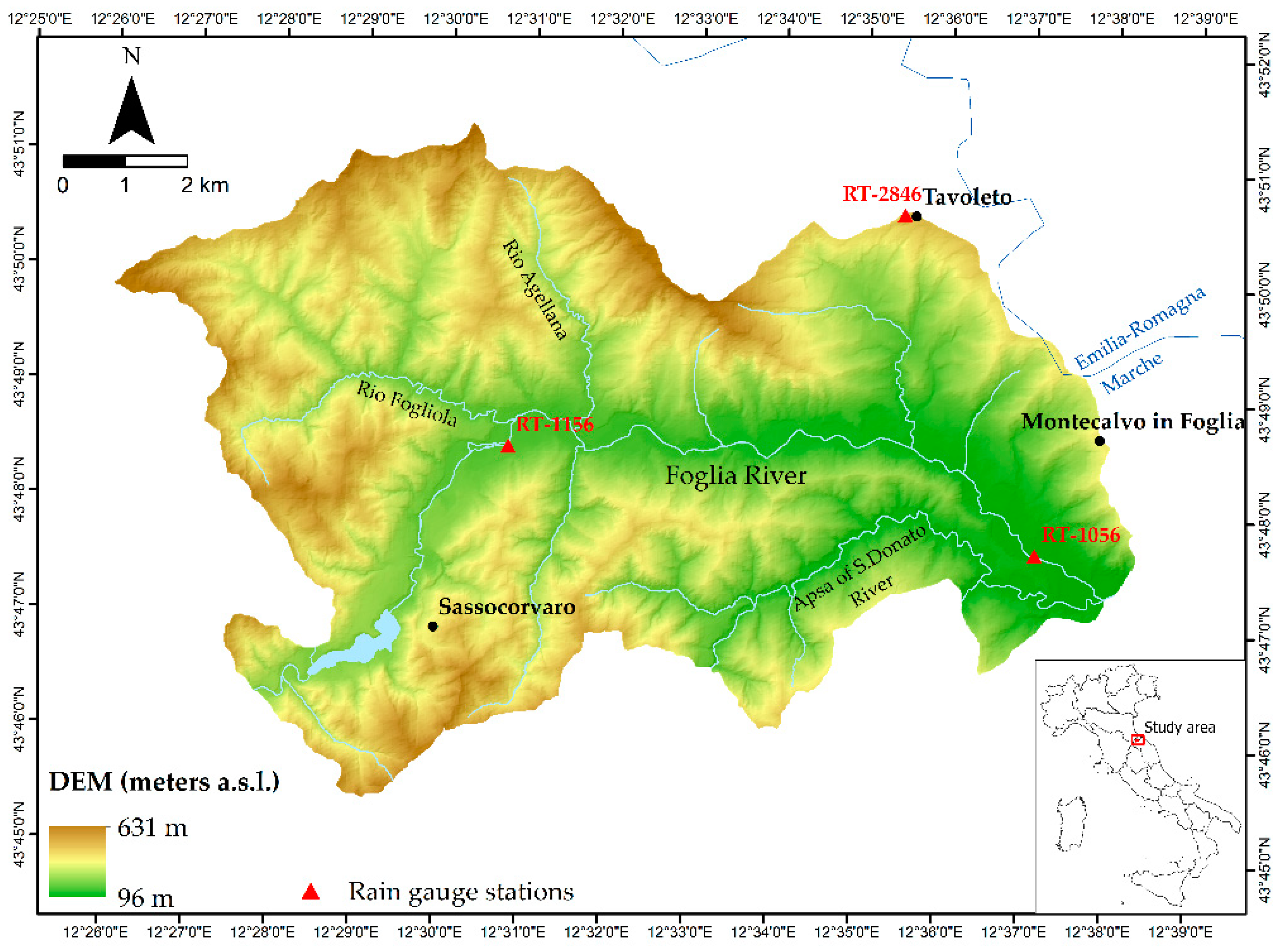
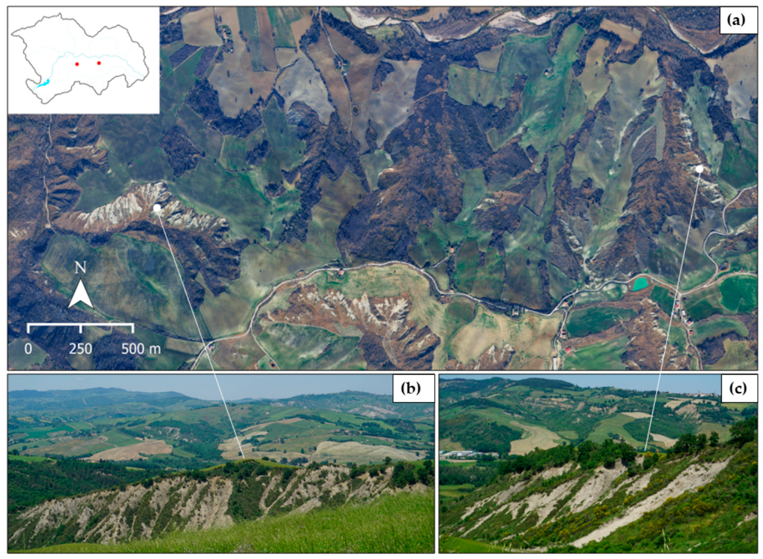
2.1. Geomorphological and Geological Setting

The study area is located in a hilly zone near the northern Apennines in the Marche region of central Italy (Figure 1). It covers approximately 102 km² within the drainage basin of the Foglia River, at elevations ranging from 96 to 625 m a.s.l. The area is traversed by the Foglia River, into which the Fogliola and Agellana rivers flow on the left bank, while the Apsa di S. Donato torrent flows in on the right bank.

The area is characterized by contrasts in the competence of the clayey–sandy outcropping rocks. The northern region includes a piedmont and a high hilly sector, where numerous landslide scarps with a high inclination occur on the marly pelitic rocks, alternating with more competent arenaceous rocks. The combination of factors, such as the composition of the outcropping rocks, contrasts in competence, tectonic action from the thrusts, and the energy of the relief, along with the landslide-supporting structure of the layers, determines the triggering of sliding and predominantly earthflow phenomena. These phenomena are largely concentrated in the high hilly sector and in the alluvial deposits near the valley floor, corresponding with clayey lithologies (Figure 2). Sometimes, these phenomena evolve into processes of concentrated runoff and degradation of the crown zone, resulting in pseudo-badlands [50]. Figure 2 illustrates the geomorphological map of the study area, although the southern sector is not represented due to the absence of data.

According to the classification proposed by Rodolfi and Frascati in 1979 [23,52], badland forms can be distinguished based on their morphological characteristics. The badlands of type A (Figure 3a,b) develop in soils with high sandy clay content. They are characterized by a dense drainage network and the typical “knife-edged” ridges, with sparse vegetation along the slopes. In contrast, the badlands of type B (Figure 3a,c) primarily originate along clay slopes affected by superficial landslides, resulting in slopes with a reduced gradient. The ridges in type B are less sharp, the drainage system is less dense, and the vegetation is more abundant compared to type A. In the study area, badlands are widespread: to the north, in the clayey soils of Val di Teva and Valle Avellana, crossed by the Fogliola and Agellana rivers; and to the south, on the slopes where the San Donato Formation outcrops, displaying more incised and steep shapes.

From the geological point of view, the area is included in the sheet 267-San Marino and 279-Urbino of the Geological Map of Italy at a scale of 1:50,000 defined in the CARG project (the Italian Geological Survey Mapping Project of Italy); the references are related to the Illustrative Notes of the Geological Map of Italy [50] (https://www.isprambiente.gov.it/Media/carg/marche.html, accessed on 1 February 2025). In particular, the geology of the area (Figure 4) includes the lithologies of the Umbria–Marche–Romagna Succession, which were deposited during the Upper Miocene, mainly represented by sandstones interbedded with clayey and marl layers. The contact with the Pleistocene lithologies of the post-evaporitic Succession of the Padano–Adriatic margin is marked by a stratigraphic unconformity. This succession is composed of mudstones interbedded with sandstone levels of the San Donato Formation and the typical marly silty clays of the Colombacci and Argille Azzurre Formations. The area also includes the Val Marecchia Nappe, consisting of the Ligurian Units deposited between the Lower Cretaceous and the Middle Eocene, along with the overlying epi-Ligurian Succession of the Oligo–Miocene epoch. The Ligurian Units are tectonic units that have undergone significant tectonic transport, as demonstrated by the highly tectonized rock masses. These are pelagic units that are predominantly clayey and calcareous pelitic. In contrast, the epi-Ligurian Succession is characterized by units that have sedimented in less deep marine environments with a greater terrigenous contribution, as evidenced by the arenaceous lithology of the bedrock and the massive gypsum banks of the Gessoso–Solfifera Formation.

In the valley floor and intravalline plains, Quaternary deposits of alluvial and eluvio-colluvial origin are identified, including Holocene sediments ranging from gravelly to clayey, and Pleistocene deposits represented by gravel with a sandy matrix. In the northern sector and the southwestern strip, the area is affected by a dense system of thrusts that play an important role in the overlap and folding of the outcropping units, as can be seen in the rocks of the Marnoso–Arenacea Formation exposed in the western sector.

Overall, in the area, the bedrock lithology is predominantly clayey, with a fair amount of sand present in the central sector. In contrast, arenaceous, calcareous and less extensive conglomeratic lithologies extend into the high hilly areas of Val di Teva and Valle Avellana. Alluvial deposits are found in the valley floor zones, while eluvio–colluvial deposits are distributed in limited extensions on the slopes. The geological data have been simplified using the lithological classes reported in

Table 2. Simplification of the lithological classes.

Lithological Classes	Geological Formations/Deposits
Sandstones	Acquaviva Formation
	Marnoso Arenacea Formation
Clays	Argille Varicolori
	Argille Azzurre Formation
	Argille di Casa i Gessi Formation
Clays and sands	Colombacci Formation
	San Donato Formation
Limestones	Monte Morello Formation
	Sillano Formation
Conglomerates, breccias	Casa Monte Sabatino Formation
Marls	Schlier
Evaporites	Gessoso–Solfifera Group
Alluvial deposits	Current alluvial deposits (Musone Synthem), terraced alluvial deposits (Musone Synthem, Matelica Synthem and Colle Ulivo-Colonia Montani Supersynthem)
Eluvial, colluvial deposits	Eluvial, colluvial deposits (Musone Synthem e Matelica Synthem)

. The resulting map of the simplified lithological classes is shown in Figure 4.

2.2. Aerial/Satellite Photos

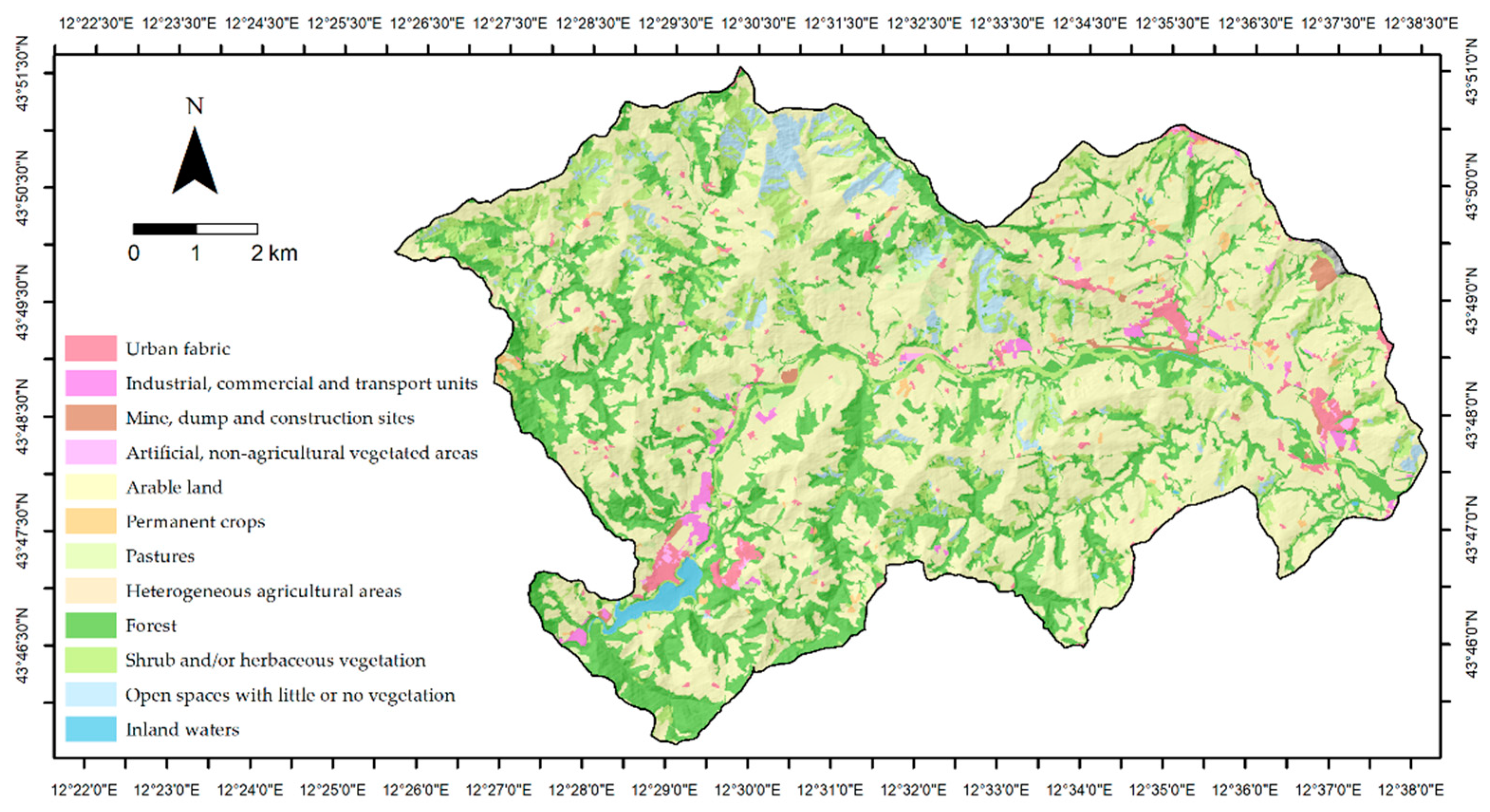
Orthophotos, available from the WMS service of the National Geoportal (http://www.pcn.minambiente.it/mattm/servizio-wms/, accessed on 1 February 2025), were utilized for the years 2006 and 2012. Google Satellite images were accessed using Google Earth Pro software and the WMS (Web Map Service) connection on the GIS platform (QGIS 3.28.0-Firenze) from 2010 to 2024. The collected orthophotos and satellite images (

Table 3. Satellite images and orthophotos used with the relative year and resolution.

Type	Year	Resolution (cm/Pixel)
Satellite images of Google Satellite	2010, 2015, 2016, 2017, 2018, 2019, 2021	30 cm
Ortophoto	2006	50 cm
Ortophoto of AGEA 1	2012	50 cm

¹ AGEA (Agenzia per le Erogazioni in Agricoltura).

) were consulted both during the mapping phase and in the study of past evolution.

2.3. Land Use

Land use information has been extracted from the land use map of the Marche region, named ADS40 2007, which represents the land functional description during the period of June–July 2007, with precision conforming to a scale of 1:10,000. This land use map was created by processing orthorectified multispectral digital images with a pixel size of 1 m, and it has a Minimum Cartographic Unit (MCU) of 0.3 hectares (three thousand square meters), allowing for an estimated average accuracy of 80% of the surface (https://www.regione.marche.it/Regione-Utile/Paesaggio-Territorio-Urbanistica/Cartografia/Repertorio/Cartausosuolo10000_2007, accessed on 1 February 2025). The land use of the study area (Figure 5) is primarily characterized by arable land (~56%), which covers the medium slopes, followed by forest areas (~26%), areas with shrub and/or herbaceous vegetation (~8%), and open spaces with little or no vegetation (~3%), corresponding to the most unstable slopes. The urbanized areas are not extensive and are primarily developed in zones adjacent to the Foglia River, forming a discontinuous urban fabric.

The land use map was simplified into six classes: water bodies, agricultural areas, urban areas, wooded areas, shrub and/or herbaceous vegetation, and bare soils or abandoned lands [16] (

Table 4. Land use classes simplified from the Marche Region’s second-level land use data.

Simplified Land Use Classes	Land Cover Classes LEVEL_2
Water bodies	Inland waters
Agricultural and/or natural areas	Permanent crops
	Pastures
	Arable land
	Heterogeneous agricultural areas
Urban areas	Mine, dump and construction sites
	Industrial, commercial, and transport units
	Artificial, non-agricultural vegetated areas
	Urban fabric
Wooded areas	Forest
Shrub and/or herbaceous vegetation	Shrub and/or herbaceous vegetation
Bare soils or abandoned lands	Open spaces with little or no vegetation

).

2.4. Pluviometric Data

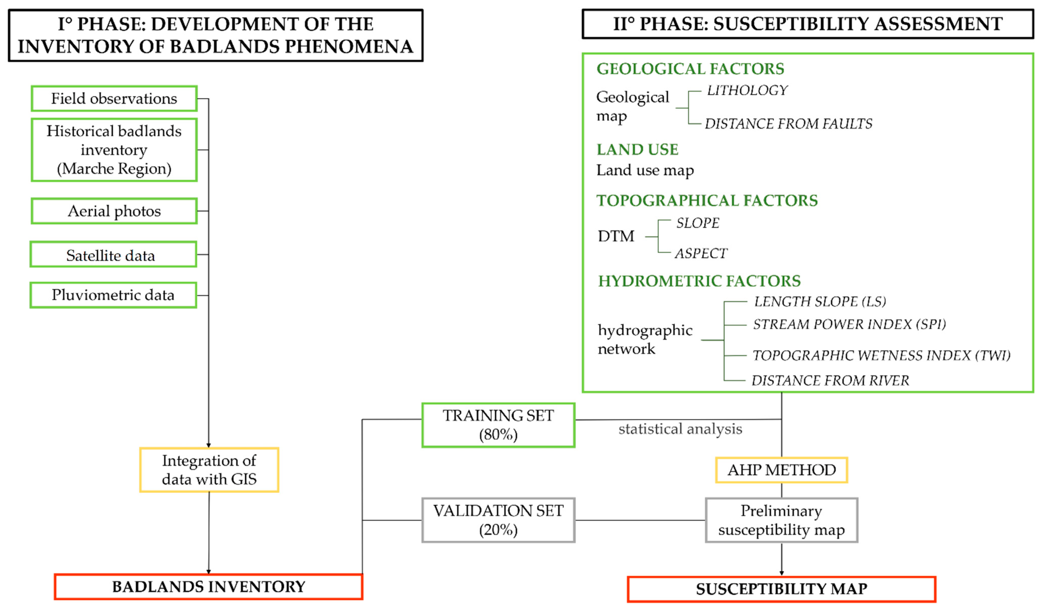
Three rain gauge stations are currently active in the study area (Figure 1), managed by the Civil Protection of the Marche Region: Ca’ Mazzasette station (RT-1056), Bronzo station (RT-1156), Tavoleto station (RT-2846).

The rainfall data were downloaded from the regional online platform called Sistema Informativo Regionale Meteo–Idro–Pluviometrico (SIRMIP; http://app.protezionecivile.marche.it/sol/indexjs.php?lang=it, accessed on 1 February 2025). They were collected only for the stations of Ca’ Mazzasette (112 m a.s.l.) and Bronzo (172 m a.s.l.), like daily precipitation (mm), from 1 January 2006 to 1 June 2023, based on the available orthophotos.

The annual rainfall patterns presented in Figure 6 reflect variable values typical of a Mediterranean climate according to the Köppen classification [53]. The most significant rainfall events occur in the autumn months (September, October, November) and the spring months (April and May), following days with medium to low daily precipitation. The high rainfall values indicate an important erosive potential, which is a consequence of the ability to remove material and modify the landscape. On predominantly clayey badland slopes, this results in increased surface runoff [54].

3. Methods

The methodology is divided into two phases (Figure 7). The first phase focuses on the development of an inventory of the badlands. The second phase is dedicated to the badlands’ susceptibility assessment.

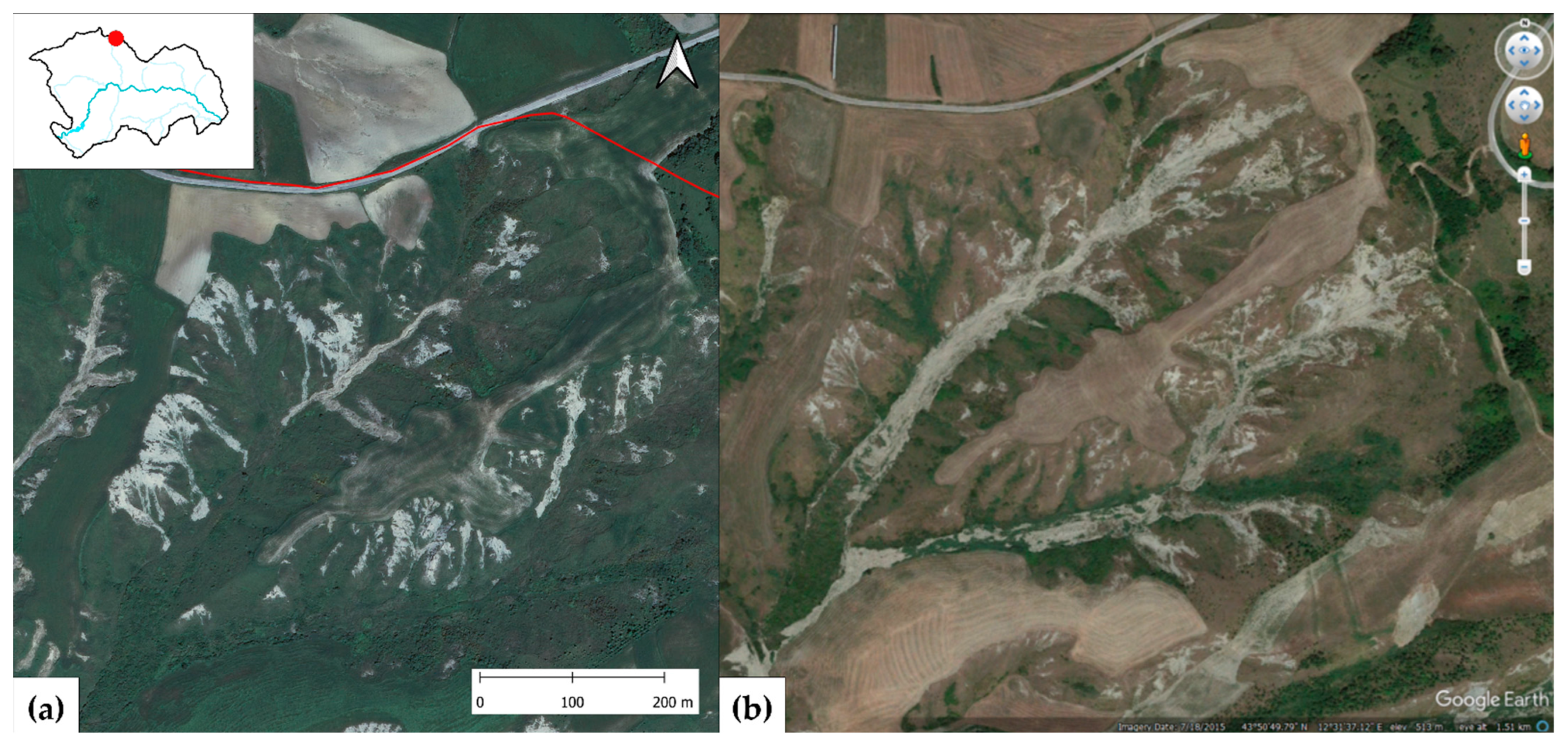
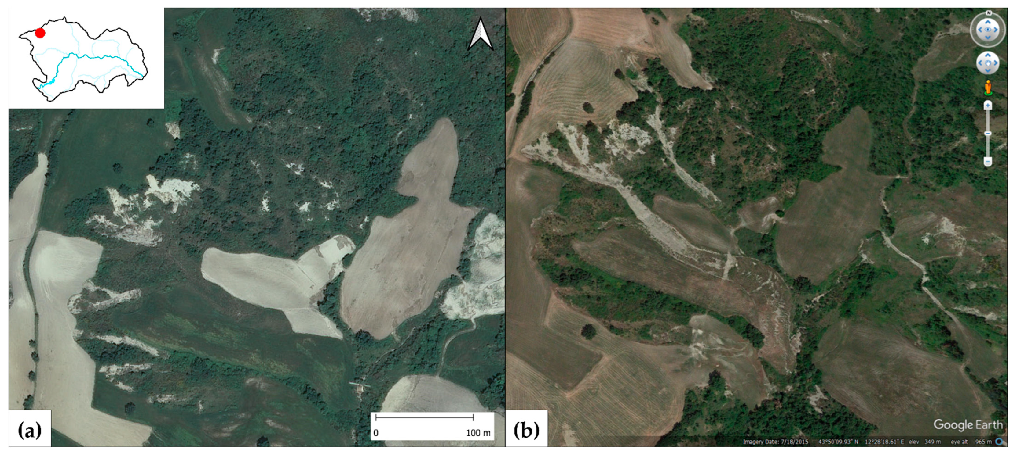
3.1. Phase I: Development of the Inventory of Badlands Phenomena

The badlands areas were mapped based on field observations, the historical inventory of the Marche Region, and aerial/satellite photos. In total, there were four field observations in the respective dates and areas:

• On 25 May 2023, the south sector of the Foglia River;
• On 12 and 16 June 2023 the slopes of Valle Avellana and the eastern part of Val di Teva;
• On 17 June 2023, the western part of Val di Teva and the slopes of Ca’ Antonio.

These data were also associated with pluviometric records to analyze the areal evolution of the badland forms in relation to major rainfall events. Then, the collected data were categorized in the GIS system according to (i) the classification proposed by Moretti and Rodolfi [23,52] and (ii) the mapping method used (i.e., field observations, the historical inventory of the Marche Region, and aerial/satellite photos).

3.2. Phase II: Susceptibility Assessment

In the second phase, the badlands’ inventory was manually randomly divided into two parts in the QGIS software version 3.16.14: training set (80% of the badlands) and validation set (20% of the badlands). The training set was used for model calibration, first by carrying out a statistical analysis of the factors predisposing to the badland genesis and then applying the AHP method for the production of the susceptibility map. The validation set has been used for model validation.

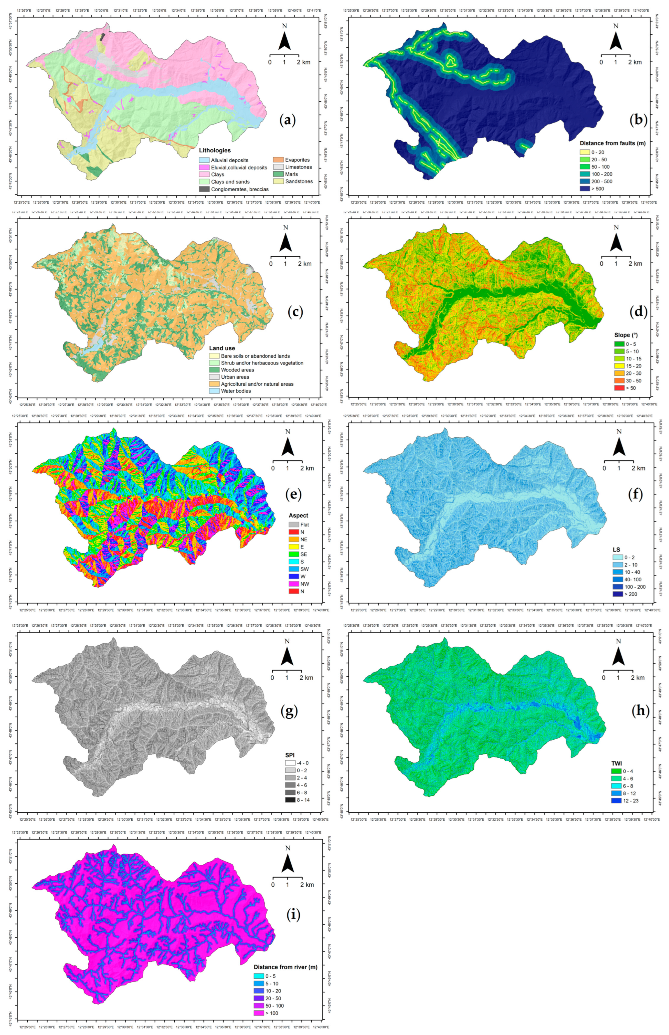
3.2.1. Predisposing Factors

Based on the state-of-the-art of previous studies, geological, land use, topographical, and hydrometric predisposing factors were considered.

The geological factor was included using the simplified lithological map obtained as explained in Section 2.1 (Figure 8a). The influence of tectonic activity was considered as a single predisposing factor, which included the Euclidean distance in meters from the faults traced in the geological map of the Marche Region; this distance was divided into six classes (Figure 8b). The DEM with a cell size of 10 m was exploited to derive three topographical parameters: slope, aspect, and curvature [55,56]. The slope was divided into seven classes (Figure 8d). The aspect included nine classes: flat areas, north (N), northeast (NE), northwest (NW), south (S), southeast (SE), southwest (SW), west (W), and east (E) (Figure 8e). The topographic presented curvature derives from the combination of the vertical curvature, defined along the line of maximum slope, with the planar curvature, calculated perpendicular to the direction of maximum slope. The curvature was divided into three classes: the concave zones correspond to cell values less than zero, the planar ones for values equal to zero and the convex ones if greater than zero. This parameter has been excluded from the following analysis due to the low relevance for the susceptibility map. Indeed, the number of badlands in the different curvature classes is the same.

The hydrological factors were included considering the length slope factor (LS) (Figure 8f), the stream power index (SPI) (Figure 8g), the topographic wetness index (TWI) (Figure 8h) and distance from rivers (Figure 8i).

Specifically, the LS addresses how topography influences soil erosion, linking the length of the contributing area to its slope. The map layer was generated using the Moore and Burch formula [57]:

$${\mathrm{L}\mathrm{S}=\left({\displaystyle \frac{\mathrm{A}\mathrm{s}}{22.14}}\right)}^{0.4}{\times \left({\displaystyle \frac{\mathrm{s}\mathrm{i}\mathrm{n}\mathsf{\beta }}{0.0896}}\right)}^{1.3},$$

(1)

where the attribute As is defined as the specific contributing area (m) and β corresponds to the slope gradient (radians). The As and β are estimated using the following formulas:

$$\mathrm{A}\mathrm{s}=\mathrm{F}\mathrm{l}\mathrm{o}\mathrm{w} \mathrm{a}\mathrm{c}\mathrm{c}\mathrm{u}\mathrm{m}\mathrm{u}\mathrm{l}\mathrm{a}\mathrm{t}\mathrm{i}\mathrm{o}\mathrm{n}\times \mathrm{c}\mathrm{e}\mathrm{l}\mathrm{l} \mathrm{s}\mathrm{i}\mathrm{z}\mathrm{e},$$

(2)

$$\mathsf{\beta }=\left(\mathrm{S}\mathrm{l}\mathrm{o}\mathrm{p}\mathrm{e} \mathrm{i}\mathrm{n}\mathrm{c}\mathrm{l}\mathrm{i}\mathrm{n}\mathrm{a}\mathrm{t}\mathrm{i}\mathrm{o}\mathrm{n}\left(°\right)\times 1.570796\right)/90.$$

(3)

The SPI defines the erosive power of water flows within a basin, relating to the extension of the drained slope and its inclination. The SPI variable was calculated using Moore’s formula [58] described as

$$\mathrm{S}\mathrm{P}\mathrm{I}=\mathrm{l}\mathrm{n}(\mathrm{A}\mathrm{s}\times \mathrm{t}\mathrm{a}\mathrm{n}\mathsf{\beta }).$$

(4)

In calculating the gradient tangent, a coefficient of 0.001 was added to the values in radians less than zero, so that the SPI value was not undefined [59].

The TWI indicates the areal distribution of soil moisture, considering the infiltration capacity of surface water as a function of the topographic characteristics of the slope. It was determined by applying the following Moore equation [58]:

$$\mathrm{T}\mathrm{W}\mathrm{I}=\mathrm{l}\mathrm{n}\left({\displaystyle \frac{\mathrm{A}\mathrm{s}}{\mathrm{t}\mathrm{a}\mathrm{n}\mathsf{\beta }}}\right).$$

(5)

The Euclidean distance from the watercourses was calculated in meters. The areas where the distance from the watercourses is shorter reflect a greater predisposition to erosion by surface runoff.

The hydrological map layers were divided into six classes, except for the TWI, which was divided into five classes, as previously proposed in the literature [16].

3.2.2. AHP Method

The AHP is a multi-criteria approach developed by Saaty in 1977, based on the determination of the best alternative in a broad context of choice, following a hierarchical structure divided into criteria, sub-criteria and alternatives. Specifically, the implementation of the AHP method includes the following steps 1 [60]:

• Selection of the explanatory variables;
• Relative importance of each explanatory variable;
• Preference scale and ratings for each explanatory variable;
• Synthetizing judgments;
• Consistency checking.

In the first step, an autocorrelation analysis is performed to verify by estimating Pearson’s correlation. Furthermore, a statistical analysis was performed on the number of badlands within class i of the parameter variable X (NX_i) and the total extent of the badlands in the classes of the aforementioned predisposing factors (AX_i). This approach allows us to identify the relevant variables. Then, each one is reclassified with predefined decimal weights following a reference scale of their importance from 0 to 5.

In the second step, the importance of each explanatory variable is established according to the literature review reported in Section 1 and about as a function of the statistical analysis results. The relative importance of each explanatory variable is assigned using a table of the judgment of the variables, expressed in a scale of scores from 1 to 9 (

Table 5. Scale of judgments defined in the work of Saaty 1987 [61].

Score	Definition	Explanation
1	Equal importance	Two factors are equally important or have the same effect
3	Moderate importance of one over another	One factor is more important than the other factor
5	Essential or strong importance	One factor is more important than the other factor
7	Very strong importance	One factor has a strong dominance over the other factor
9	Extreme importance	One factor has the highest order of dominance over another
2, 4, 6, 8	Intermediate importance between two scores	When compromise is needed

) [61].

The scores form the structure of square matrix A of possible decisions (step 3). Matrix A corresponds to an eigenvector w which defines the order of the predisposing factors, such that there is a value λ_max indicated as the principal eigenvalue of A (step 4):

$$Aw={\lambda }_{max}w.$$

(6)

In the last step, the consistency of matrix A is defined, which corresponds to its reliability in the overall assessments and attributed scores. It is calculated using the Consistency Index (CI):

$$CI={\displaystyle \frac{{\lambda }_{\max }-n}{n-1}},$$

(7)

where n represents the number of criteria evaluated in the decision problem.

Subsequently, the index of matrix A is then related to the CI of a random matrix, defining the Consistency Ratio (CR). If CR is less than or equal to 10%, the judgments are valid; if greater than 10%, we have an inconsistent matrix, which is followed by a revision of the judgments.

3.2.3. Validation

Finally, the susceptibility map was validated by comparing the predicted susceptibility classes with the badlands of the validation set of the inventory. The susceptibility map is classified into five susceptibility classes using the natural breaks classification method [54] and an inspection of the total number of badlands for each susceptibility class is performed.

A sensitivity analysis was integrated into the validation in order to estimate the accuracy of the prediction model.

4. Results

4.1. Badlands Inventory

A total of 276 badland areas were mapped using different datasets described in Section 3.1, covering approximately 5.8% of the area (about 5.9 km²) (Figure 9a).

There are 46 type A badlands, covering 1.6 km², and 230 type B badlands, with an extent of 4.3 km² (Figure 9b).

The relationship between major rainfall occurrences and evolution of slope stability conditions was analyzed in two different areas by a multitemporal study of aerial and satellite photos. In particular, the rainfall events of 2012 and 2013 were considered, consulting the 2012 orthophoto for the pre-event situation and the 2015 Google Earth satellite image for the post-event situation. The two sample areas were located in (a) Valle Avellana, characterized by type A badland morphologies with medium-high slopes and clayey lithologies (Figure 10), and (b) Ca’ Antonio, having type B badland morphologies with medium-high slopes and clayey–sandy lithologies (Figure 11).

In the first area, the erosive action of the rain is evident: removal of material deposited at the base of the badland, slight smoothing of the badlands ridges, earthflows involving the main sector of the drainage network of the badland basins (Figure 10).

In the second area, rainfall over time has led to an increase in surface runoff, triggering two earthflow phenomena, one of which is characterized by a larger surface area at the valley floor (Figure 11).

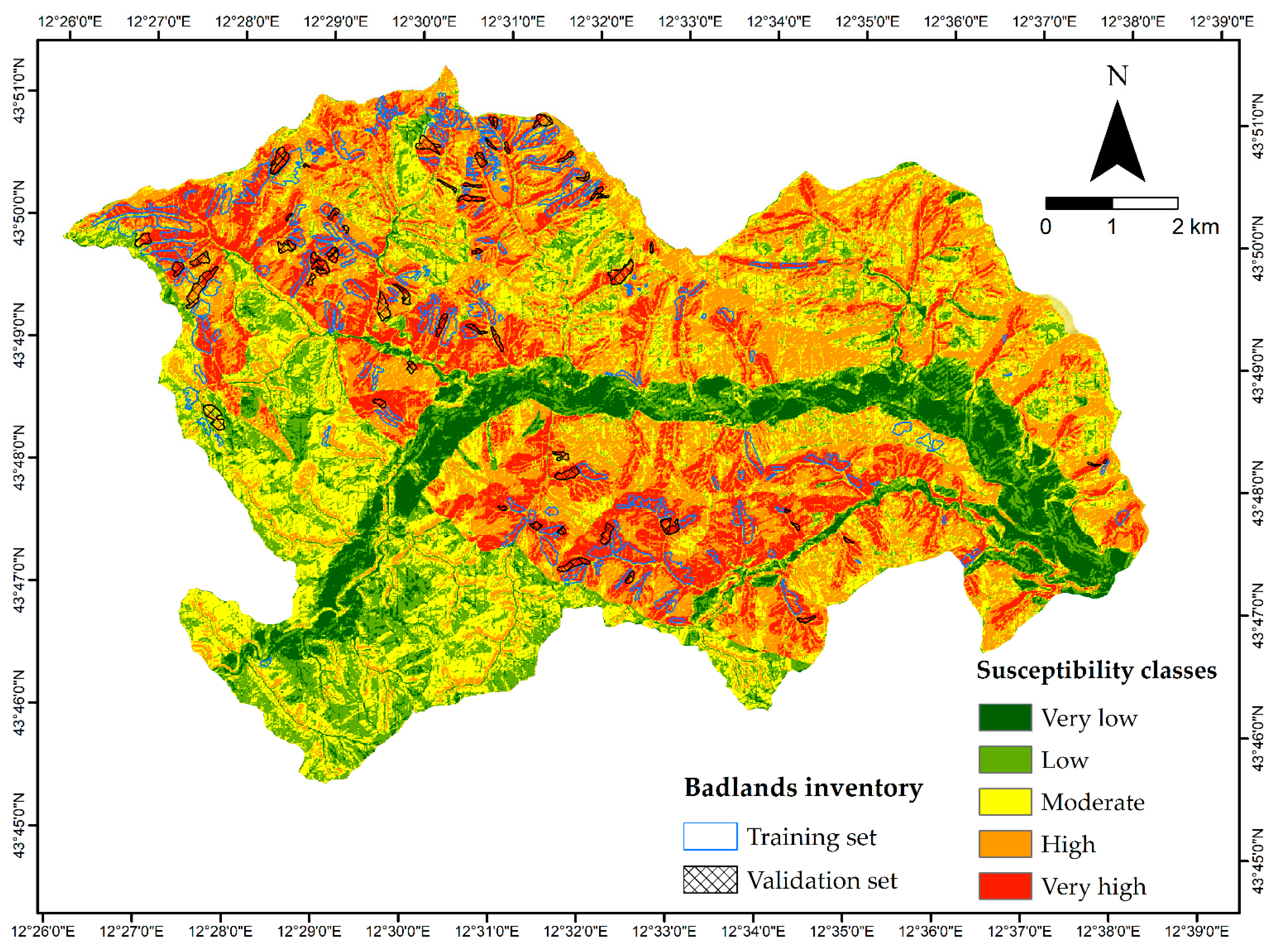
4.2. Susceptibility Mapping

4.2.1. Statistical Analysis

The results of the statistical analysis (

Table 6. Results of the statistical analysis and the weights attributed for the classes of each predisposing factor chosen in the susceptibility assessment.

PREDISPOSING FACTORS	NUMBER OF BADLANDS	AREA (km2)	ASSIGNED WEIGHT	NORMALIZED CLASS WEIGHTS
LITHOLOGY
Sandstones	13	0.53	2	0.13
Clays	134	2.442	4	0.27
Clays and sands	95	2.98	5	0.33
Limestones	20	0.663	3	0.2
Conglomerates and breccias	5	0.189	1	0.07
Alluvial deposits	4	0.04	1	0.07
Eluvial, colluvial deposits	1	0.12	1	0.07
Evaporites	4	0.13	1	0.07
Marls	3	0.06	1	0.07
DISTANCE FROM FAULTS (m)
0–20	34	1.22	1	0.07
20–50	42	1.39	1	0.07
50–100	58	1.63	2	0.13
100–200	75	1.95	3	0.2
200–500	91	2.19	4	0.27
>500	117	2.63	5	0.33
LAND USE
Water bodies	0	0.00	0	0
Agricultural and/or natural areas	145	3.92	4	0.27
Urban areas	0	0.00	0	0
Wooded areas	133	3.67	3	0.2
Shrub and/or herbaceous vegetation	170	4.26	5	0.33
Bare soils or abandoned lands	131	3.20	2	0.13
SLOPE (°)
0–5	54	2.10	2	0.13
5–10	163	4.30	3	0.2
10–15	210	4.66	5	0.33
15–20	220	4.69	5	0.33
20–30	221	4.69	5	0.33
30–50	206	4.65	4	0.27
>50	20	0.76	1	0.07
ASPECT
N	122	3.03	4	0.27
NE	96	2.74	2	0.13
E	125	3.10	4	0.27
SE	136	3.34	5	0.33
S	138	3.64	5	0.33
SO	123	3.21	4	0.27
O	106	2.77	3	0.2
NO	76	2.01	1	0.07
LS
0–2	221	4.69	5	0.33
2–10	221	4.69	5	0.33
10–40	220	4.69	5	0.33
40–100	116	6.57	3	0.2
100–200	11	0.26	2	0.13
>200	1	0.06	1	0.07
SPI
−4–0	48	1.72	1	0.07
0–2	221	4.69	5	0.33
2–4	221	4.69	5	0.33
4–6	215	4.67	4	0.27
6–8	154	4.20	3	0.2
8–14	60	2.27	2	0.13
TWI
0–4	221	4.69	5	0.33
4–6	221	4.69	5	0.33
6–8	214	4.67	4	0.27
8–12	163	4.33	2	0.13
12–23	27	1.56	1	0.07
DISTANCE FROM RIVERS (m)
0–5	134	3.67	2	0.13
5–10	170	4.16	3	0.2
10–20	184	4.36	4	0.27
20–50	194	4.43	5	0.33
50–100	177	4.38	3	0.2
>100	111	3.16	1	0.07

) show the influence of lithology in the genesis of the badlands, underlining how the fine-grained composition of the soils determines a fundamental role in the setting of the accelerated erosion process. Clay lithologies record a greater number of badlands, followed by lithologies characterized by the alternance of clay and sand that implies the definition of more accentuated morphological characters on steep slopes. Differently, the distance from certain faults does not appear to be important. The erosion process tends to affect all the vegetated surfaces of the study area. It affects the surfaces with shrubby and/or herbaceous vegetation. A higher number of badlands is observed in 20–30° slopes [10]. In addition, it has also to be highlighted the relevant influence of the southern exposure (southeast, south, southwest), where temperatures are higher, the thermal shock is greater, and the water content is lower. The curvature was discarded from the susceptibility evaluation, as it does not appear to be relevant to the badlands distribution.

In the studied area, badlands tend to affect areas with low LS values, corresponding to medium slopes, close to steep slopes and watercourses. Regarding the SPI, badlands tend to concentrate in areas with values greater than 0 where the erosive power is limited, to a lesser extent the classes with high SPI values. The results obtained from the analysis of the TWI show badland occurrence is higher in soils with a poor infiltration capacity relative to low values of the humidity index that become the site of the linear erosion process. Finally, the number of badlands and areas is visibly greater for shorter distances from watercourses, forming a very dense drainage network.

As observed in Table 6, each predisposing factor was reclassified by assigning to each class a weight in the form of a predefined decimal value, following a reference scale from 0 to 5. The lower values correspond to a lesser influence of the predisposing factors.

4.2.2. AHP Method Matrix

The consistency of the matrix itself with the CR was calculated and the relative susceptibility map was produced only for a CR value lower than 0.1. It should be noted that, in order to identify the most performing susceptibility model, three different susceptibility models were produced, of which only the data of the most representative model are reported in this work. The matrix and the importance scale of the predisposing factors are reported in

Table 7. Matrix and weights attributed to the predisposing factors. The no values fields represent the assigned transposed values.

Factors	Lithology	Distance from Faults	Land Use	Slope	Aspect	Distance from Rivers	LS	SPI	TWI
Lithology	1	5	5	2	2	2	2	3	3
Distance from faults		1	0.5	0.125	0.125	0.125	0.125	0.125	0.125
Land use			1	0.5	0.5	0.5	0.5	0.5	0.5
Slope				1	2	2	2	2	3
Aspect					1	2	2	2	3
Distance from rivers						1	2	2	3
LS							1	2	3
SPI								1	2
TWI									1

and

Table 8. Importance scale derived from the matrix in Table 7.

Lithology	22.19
Slope	17.35
Aspect	14.89
Distance from rivers	12.79
LS	10.98
SPI	8.48
TWI	6.40
Land use	5.05
Distance from faults	1.83

. The resulting CR value for the reported matrix is equal to 0.053.

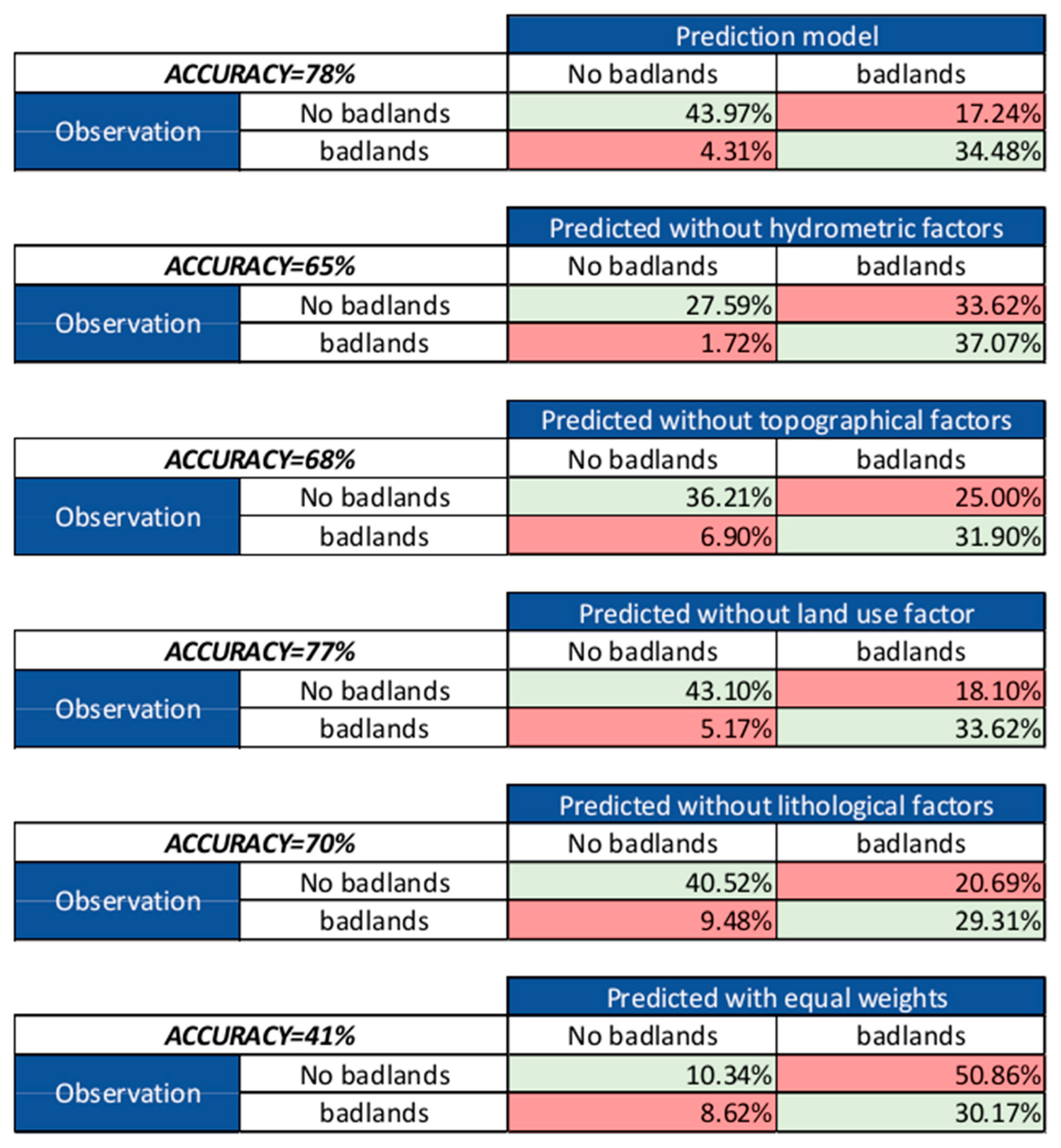
4.2.3. Validation of the Susceptibility Map

The susceptibility map is shown in Figure 12. In most cases, the high susceptibility areas include the badlands of the validation (

Table 9. Results of the validation. The total number of badlands in the validation set is 55.

Susceptibility Classes	Class Values	Number of Badlands
Very low	1.6–2.9	0
Low	2.9–3.4	0
Moderate	3.4–3.9	1
High	3.9–4.3	12
Very high	4.3–5	42

). For this reason, the developed model can be considered representative of the susceptibility prediction to badland phenomena in the studied area. The map produced reflects the interaction of different factors, highlighting a particular influence of lithology, slope and exposure.

Furthermore, a sensitivity analysis was performed to evaluate the accuracy of the prediction model and the performance of the assigned weights and selected predisposing factors. Five additional scenarios compared to the prediction model have been defined, as follows:

• Scenario: zero weights to hydrometric factors;
• Scenario: zero weight to topographical factors;
• Scenario: zero weight to land use factor;
• Scenario: zero weight to lithological factors;
• Scenario: same weights for all AHP criteria.

In this case, the validation dataset also includes additional random points of no badlands locations. This approach is exploited to verify the overestimation of the developed susceptibility map. The results give insight into the role of the selected variables and the higher accuracy of the proposed prediction model that reaches values of 78%. The lower accuracy (41%) is observed considering equal weight to all variables (Figure 13). This evidence confirms the reliability of susceptibility mapping.

5. Discussion

The produced badland inventory was useful for the integration of recent geomorphological information in an area where the geomorphological cartography is partially missing. Approximately 34% of the total area was not previously mapped. By comparing the badland areas with the major recorded rainfall events, it is possible to confirm that the badland erosive phenomena are strictly linked to the erosive action of rain, which influences the development of the vegetation cover, the surface runoff [62], and the triggering earthflow phenomena depend. Moreover, our analysis is externally validated by recent field observations during a precipitation event in May 2023 with a maximum daily precipitation of 108 mm.

The statistical analysis between the distribution of the badlands and ten predisposing factors shows a local control of the lithology, slope, and exposure.

These results are in agreement with those obtained by other authors [16,20,33], although the land use seems to be less relevant in the investigated area. In contrast to the previous study conducted by Vergari et al., 2015 [16,20,33], our research has taken different predisposing factors. Specifically, we have incorporated land use, proximity to fault lines, and rivers as critical variables in our analysis. Furthermore, the curvature has been excluded from our analysis. The same difference is observed with respect to the work proposed by Bianchini et al., 2016 [16,20,33]. Also for the first time, the distance from fault has been considered in the badland susceptibility in order to take into account the tectonic setting as reported by Nisio et al., 1996 [16,20,33].

The susceptibility assessment was carried out using the AHP multicriteria analysis method. The validated result shows an overestimation of the extension of the badlands areas, and this aspect is also identified for other susceptibility models [16,63]. Given the results of the validation phase, the moderate degree of overestimation and the optimal level of discretization of the areas, the obtained susceptibility model is considered representative of the analyzed territory. The areas characterized by high and very high badland susceptibility correspond to sandy clay slopes with a medium–high slope value. These are mainly located near the main tributaries of the Foglia River with a prevalent exposure towards the southern quadrants. On the contrary, the areas with low susceptibility are related to the riverbed zones of the major watercourses and to the area characterized by competent lithologies.

As reported by previous authors, the spatial and temporal variability of erosion processes and the complex spatial and temporal connections at the catchment scale [64] and high variability in erosion and sediment yield have been observed across scales. Furthermore, badlands appear to be more complex than initially assumed [65]. Therefore, even if the paper proposes a reproducible procedure, some local calibration of the selection of the predisposing factors and their weight should be carried out in further applications of the methodology in different geological, climatic, and topographical conditions.

6. Conclusions

This research has dealt with the development of a methodology for studying badlands in a portion of the Foglia River basin in the province of Pesaro–Urbino (Marche region, Central Italy). For the first time, an inventory of the badlands has been developed for the study area by integrating in situ, cartographic maps and aerial/satellite photos.

The proposed approach led to predict the badlands susceptibility at a basin scale. Susceptibility mapping has been obtained using the AHP method and considering a selection of nine geologic, land use, topographical, and hydrometric variables. Five grades of badlands susceptibility have been mapped from very low to very high.

The reliability of the achieved results has been checked using a validation set that represents 20% of the badland inventories.

It emerged that the most susceptible areas are characterized by clayey–sandy lithologies, medium-high slopes exposed towards the southern quadrants and close to the tributaries of the Foglia River.

Considering the good results gathered by the validation procedure, the proposed methodology can be extended to other areas characterized by the presence of badlands. The badlands inventory and susceptibility map are key tools for identifying areas potentially prone to linear erosion. These products are valuable for the planning and management of land use, as they help prevent and mitigate the risks associated with slope instability.

References

1. Alexander, D.E. I Calanchi-Accelerated Erosion in Italy. Geography 1980, 65, 95–100. [Google Scholar] [CrossRef]
2. Gallart, F.; Solé-Benet, A.; Puigdefabragas, J.; Lazaro, R. Badland Systems in the Mediterranean. In Dryland Rivers: Hydrology and Geomorphology of Semi-Arid Channels; John Wiley & Sons: Hoboken, NJ, USA, 2002; pp. 299–326. [Google Scholar]
3. Dramis, F.; Gentili, B.; Coltorti, M.; Cherubini, C. Osservazioni Geomorfologiche Sui Calanchi Marchigiani: Geomorphological Observations on Badlands in the Marche Region. Geogr. Fis. Din. Quat. 1982, 5, 38–45. [Google Scholar]
4. Bryan, R.; Yair, A. Badland Geomorphology and Piping; Geo Books, 1982; ISBN 978-0-86094-113-2. [Google Scholar]
5. Gallart, F.; Marignani, M.; Pérez-Gallego, N.; Santi, E.; Maccherini, S. Thirty Years of Studies on Badlands, from Physical to Vegetational Approaches. A Succinct Review. Catena 2013, 106, 4–11. [Google Scholar] [CrossRef]
6. Avcıoğlu, A.; Görüm, T.; Akbaş, A.; Moreno-de las Heras, M.; Yıldırım, C.; Yetemen, Ö. Regional Distribution and Characteristics of Major Badland Landscapes in Turkey. Catena 2022, 218, 106562. [Google Scholar] [CrossRef]
7. Arabameri, A.; Pradhan, B.; Rezaei, K.; Conoscenti, C. Gully Erosion Susceptibility Mapping Using GIS-Based Multi-Criteria Decision Analysis Techniques. Catena 2019, 180, 282–297. [Google Scholar] [CrossRef]
8. Torra, O.; Hürlimann, M.; Puig-Polo, C.; Moreno-de-Las-Heras, M. Assessment of Badland Susceptibility and Its Governing Factors Using a Random Forest Approach. Application to the Upper Llobregat River Basin and Catalonia (Spain). Environ. Res. 2023, 237, 116901. [Google Scholar] [CrossRef] [PubMed]
9. Nisio, S.; Prestininzi, A.; Mugnozza, G.S. Della Fascia Periadriatica Abruzzese: Quadro Morfotettonico e Loro Caratterizzazione. Studi Geol. Camerti 1996, 14, 29–45. [Google Scholar]
10. Azzi, G. I Fenomeni Della Erosione Nelle Argille Azzurre Del Pliocene Nel Bacino Del Santerno (Romagna). Boll. Della Soc. Geogr. Ital. 1912, 111–142. [Google Scholar]
11. Castiglioni, B. Osservazioni Sui Calanchi Appenninici. Boll. Della Soc. Geol. Ital. 1933, 52, 357–360. [Google Scholar]
12. Battaglia, S.; Leoni, L.; Sartori, F. Mineralogical and Grain Size Composition of Clays Developing Calanchi and Biancane Erosional Landforms. Geomorphology 2003, 49, 153–170. [Google Scholar] [CrossRef]
13. Buccolini, M.; Gentili, B.; Materazzi, M.; Aringoli, D.; Pambianchi, G.; Piacentini, T. Human Impact and Slope Dynamics Evolutionary Trends in the Monoclinal Relief of Adriatic Area of Central Italy. Catena 2007, 71, 96–109. [Google Scholar] [CrossRef]
14. Guzzetti, F.; Reichenbach, P.; Ardizzone, F.; Cardinali, M.; Galli, M. Estimating the Quality of Landslide Susceptibility Models. Geomorphology 2006, 81, 166–184. [Google Scholar] [CrossRef]
15. Vergari, F. Assessing Soil Erosion Hazard in a Key Badland Area of Central Italy. Nat. Hazards 2015, 79, 71–95. [Google Scholar] [CrossRef]
16. Bianchini, S.; Del Soldato, M.; Solari, L.; Nolesini, T.; Pratesi, F.; Moretti, S. Badland Susceptibility Assessment in Volterra Municipality (Tuscany, Italy) by Means of GIS and Statistical Analysis. Environ. Earth Sci 2016, 75, 889. [Google Scholar] [CrossRef]
17. Farabollini, P.; Gentili, B.; Pambianchi, G. Contributo Allo Studio Dei Calanchi: Due Aree Campione Nelle Marche. Studi Geol. Camerti. Nuova Ser. 1992, 12, 105–115. [Google Scholar]
18. Buccolini, M.; Coco, L. MSI (Morphometric Slope Index) for Analyzing Activation and Evolution of Calanchi in Italy. Geomorphology 2013, 191, 142–149. [Google Scholar] [CrossRef]
19. Cocco, S.; Brecciaroli, G.; Agnelli, A.; Weindorf, D.; Corti, G. Soil Genesis and Evolution on Calanchi (Badland-like Landform) of Central Italy. Geomorphology 2015, 248, 33–46. [Google Scholar] [CrossRef]
20. Bufalini, M.; Omran, A.; Bosino, A. Assessment of Badlands Erosion Dynamics in the Adriatic Side of Central Italy. Geosciences 2022, 12, 208. [Google Scholar] [CrossRef]
21. Passerini, G. Influenze Della Immersione Degli Strati Ed Influenze Dell’orientamento Dei Versanti Sulla Degradazione Delle Argille Plioceniche; Tipografica Sabbadini: Udine, Italy, 1937; Volume 56. [Google Scholar]
22. Sdao, G.; Simone, A.; Vittorini, S. Osservazioni Geomorfologiche Su Calanchi e Biancane in Calabria: Geomorphological Observations on Calanchi and Biancane in the Calabria Region. Geogr. Fis. Din. Quat. 1984, 7, 10–16. [Google Scholar]
23. Moretti, S.; Rodolfi, G. A Typical “Calanchi” Landscape on the Eastern Apennine Margin (Atri, Central Italy): Geomorphological Features and Evolution. Catena 2000, 40, 217–228. [Google Scholar] [CrossRef]
24. Piccarreta, M.; Capolongo, D.; Bentivenga, M.; Pennetta, L. Influenza Delle Precipitazioni e Dei Cicli Umido-Secco Sulla Morfogenesi Calanchiva in Un’area Semi-Arida Della Basilicata (Italia Meridionale). Suppl. Geogr. Fis. Din. Quat. 2005, 7, 281–289. [Google Scholar]
25. De Santis, F.; Giannossi, M.L.; Medici, L.; Summa, V.; Tateo, F. Impact of Physico-Chemical Soil Properties on Erosion Features in the Aliano Area (Southern Italy). Catena 2010, 81, 172–181. [Google Scholar] [CrossRef]
26. Vergari, F.; Della Seta, M.; Del Monte, M.; Barbieri, M. Badlands Denudation “Hot Spots”: The Role of Parent Material Properties on Geomorphic Processes in 20-Years Monitored Sites of Southern Tuscany (Italy). Catena 2013, 106, 31–41. [Google Scholar] [CrossRef]
27. Pulice, I.; Di Leo, P.; Robustelli, G.; Scarciglia, F.; Cavalcante, F.; Belviso, C. Control of Climate and Local Topography on Dynamic Evolution of Badland from Southern Italy (Calabria). Catena 2013, 109, 83–95. [Google Scholar] [CrossRef]
28. Torri, D.; Rossi, M.; Brogi, F.; Marignani, M.; Bacaro, G.; Santi, E.; Tordoni, E.; Amici, V.; Maccherini, S. Badlands and the Dynamics of Human History, Land Use, and Vegetation Through Centuries. In Badlands Dynamics in a Context of Global Change; Elsevier: Amsterdam, The Netherlands, 2018; pp. 111–153. ISBN 978-0-12-813054-4. [Google Scholar]
29. Rossi, M.; Torri, D.; De Geeter, S.; Cremer, C.; Poesen, J. Topographic Thresholds for Gully Head Formation in Badlands. Earth Surf. Process. Landf. 2022, 47, 3558–3587. [Google Scholar] [CrossRef]
30. Anseimi, B.; Crovato, C.; D’Angelo, L.; Grauso, S. The Badlands of Atri (Abruzzo, Central Italy): Mineralogical, Geotechnical and Geomorphological Characters. Alp. Mediterr. Quat. 1994, 7, 145–158. [Google Scholar]
31. Liberti, M.; Simoniello, T.; Carone, M.T.; Coppola, R.; D’Emilio, M.; Macchiato, M. Mapping Badland Areas Using LANDSAT TM/ETM Satellite Imagery and Morphological Data. Geomorphology 2009, 106, 333–343. [Google Scholar] [CrossRef]
32. Battaglia, S.; Leoni, L.; Rapetti, F.; Spagnolo, M. Dynamic Evolution of Badlands in the Roglio Basin (Tuscany, Italy). Catena 2011, 86, 14–23. [Google Scholar] [CrossRef]
33. Bosino, A.; Omran, A.; Maerker, M. Identification, Characterisation and Analysis of the Oltrepo Pavese Calanchi in the Northern Apennines (Italy). Geomorphology 2019, 340, 53–66. [Google Scholar] [CrossRef]
34. Coratza, P.; Parenti, C. Controlling Factors of Badland Morphological Changes in the Emilia Apennines (Northern Italy). Water 2021, 13, 539. [Google Scholar] [CrossRef]
35. Farabegoli, E.; Agostini, C. Identification Ofcalanco, a Badland Landform in the Northern Apennines, Italy. Earth Surf. Process. Landf. 2000, 25, 307–318. [Google Scholar] [CrossRef]
36. Buccolini, M.; Coco, L. The Role of the Hillside in Determining the Morphometric Characteristics of “Calanchi”: The Example of Adriatic Central Italy. Geomorphology 2010, 123, 200–210. [Google Scholar] [CrossRef]
37. Buccolini, M.; Coco, L.; Cappadonia, C.; Rotigliano, E. Relationships between a New Slope Morphometric Index and Calanchi Erosion in Northern Sicily, Italy. Geomorphology 2012, 149–150, 41–48. [Google Scholar] [CrossRef]
38. Caraballo-Arias, N.A.; Ferro, V. Assessing, Measuring and Modelling Erosion in Calanchi Areas: A Review. J. Agric. Eng. 2016, 47, 181. [Google Scholar] [CrossRef]
39. Cappadonia, C.; Coco, L.; Buccolini, M.; Rotigliano, E. From Slope Morphometry to Morphogenetic Processes: An Integrated Approach of Field Survey, Geographic Information System Morphometric Analysis and Statistics in Italian Badlands. Land Degrad. Dev. 2016, 27, 851–862. [Google Scholar] [CrossRef]
40. Caraballo-Arias, N.A.; Di Stefano, C.; Ferro, V. Morphological Characterization of Calanchi (Badland) Hillslope Connectivity. Land Degrad. Dev. 2018, 29, 1190–1197. [Google Scholar] [CrossRef]
41. Bosino, A.; Szatten, D.A.; Omran, A.; Crema, S.; Crozi, M.; Becker, R.; Bettoni, M.; Schillaci, C.; Maerker, M. Assessment of Suspended Sediment Dynamics in a Small Ungauged Badland Catchment in the Northern Apennines (Italy) Using an in-Situ Laser Diffraction Method. Catena 2022, 209, 105796. [Google Scholar] [CrossRef]
42. Clarke, M.L.; Rendell, H.M. Process–Form Relationships in Southern Italian Badlands: Erosion Rates and Implications for Landform Evolution. Earth Surf. Process. Landf. 2006, 31, 15–29. [Google Scholar] [CrossRef]
43. Ciccacci, S.; Galiano, M.; Roma, M.A.; Salvatore, M.C. Morphological Analysis and Erosion Rate Evaluation in Badlands of Radicofani Area (Southern Tuscany—Italy). Catena 2008, 74, 87–97. [Google Scholar] [CrossRef]
44. Ciccacci, S.; Galiano, M.; Roma, M.A.; Salvatore, M.C. Morphodynamics and Morphological Changes of the Last 50 Years in a Badland Sample Area of Southern Tuscany (Italy). Z. Fur Geomorphol. 2009, 53, 273–297. [Google Scholar] [CrossRef]
45. Della Seta, M.; Del Monte, M.; Fredi, P.; Lupia Palmieri, E. Space–Time Variability of Denudation Rates at the Catchment and Hillslope Scales on the Tyrrhenian Side of Central Italy. Geomorphology 2009, 107, 161–177. [Google Scholar] [CrossRef]
46. Capolongo, D.; Pennetta, L.; Piccarreta, M.; Fallacara, G.; Boenzi, F. Spatial and Temporal Variations in Soil Erosion and Deposition Due to Land-levelling in a Semi-arid Area of Basilicata (Southern Italy). Earth Surf. Process. Landf. 2008, 33, 364–379. [Google Scholar] [CrossRef]
47. Castaldi, F.; Chiocchini, U. Effects of Land Use Changes on Badland Erosion in Clayey Drainage Basins, Radicofani, Central Italy. Geomorphology 2012, 169–170, 98–108. [Google Scholar] [CrossRef]
48. Bollati, I.; Vergari, F.; Del Monte, M.; Pelfini, M. Multitemporal Dendrogeomorphological Analysis of Slope Instability in Upper Orcia Valley (Southern Tuscany, Italy). Geogr. Fis. Din. Quat. 2016, 39, 105–120. [Google Scholar]
49. TINITALY, A Digital Elevation Model of Italy with a 10 Meters Cell Size—ISTITUTO NAZIONALE DI GEOFISICA E VULCANOLOGIA. Available online: https://data.ingv.it/dataset/185#additional-metadata (accessed on 23 October 2024).
50. Cornamusini, G.; Conti, P.; Bonciani, F.; Callegari, I.; Carmignani, L.; Martelli, L.; Quagliere, S. Note Illustrative Della Carta Geologica d’Italia Alla Scala 1: 50.000 “Foglio 267-San Marino”; Servizio Geologico d’Italia: Rome, Italy, 2009. [Google Scholar]
51. Regione Marche Geomorphological Map of the Marche Region-Sheet 267 San Marino (Sections CTD 267100, CTD 267110, CTD 267140, CTD 267150, CTD 267160) 2001. Available online: https://www.regione.marche.it/Regione-Utile/Paesaggio-Territorio-Urbanistica/Cartografia/Repertorio/Cartageomorfologicaregionale10000 (accessed on 1 February 2025).
52. Rodolfi, G.; Frascati, F. Cartografia Di Base per La Programmazione Degli Interventi in Aree Marginali Area Rappresentativa Dell’alta Valdera: Memorie Illustrative Della Carta Geomorfologica Con Una Nota Sulla Costituzione Geolitologica Dell’area; Tipografia R. Coppini: Firenze, Italy, 1979. [Google Scholar]
53. Köppen, W. Das Geographische System der Klimate; Gebrüdcr Borntraeger: Berlin, Germany, 1936. [Google Scholar]
54. Wolman, M.G.; Miller, J.P. Magnitude and Frequency of Forces in Geomorphic Processes. J. Geol. 1960, 68, 54–74. [Google Scholar] [CrossRef]
55. Wilson, J.P.; Gallant, J.C. (Eds.) Terrain Analysis: Principles and Applications; Wiley: New York, NY, USA, 2000; ISBN 978-0-471-32188-0. [Google Scholar]
56. Morelli, S.; Bonì, R.; De Donatis, M.; Marino, L.; Pappafico, G.F.; Francioni, M. A Low-Cost and Fast Operational Procedure to Identify Potential Slope Instabilities in Cultural Heritage Sites. Remote Sens. 2023, 15, 5574. [Google Scholar] [CrossRef]
57. Moore, I.D.; Burch, G.J. Physical Basis of the Length-Slope Factor in the Universal Soil Loss Equation. Soil Sci. Soc. Am. J. 1986, 50, 1294–1298. [Google Scholar] [CrossRef]
58. Moore, I.D.; Grayson, R.B.; Ladson, A.R. Digital Terrain Modelling: A Review of Hydrological, Geomorphological, and Biological Applications. Hydrol. Process. 1991, 5, 3–30. [Google Scholar] [CrossRef]
59. Chowdhury, M.S. Modelling Hydrological Factors from DEM Using GIS. MethodsX 2023, 10, 102062. [Google Scholar] [CrossRef]
60. Saaty, T.L. Decision Making with the Analytic Hierarchy Process. IJSSCI 2008, 1, 83. [Google Scholar] [CrossRef]
61. Saaty, R.W. The Analytic Hierarchy Process—What It Is and How It Is Used. Math. Model. 1987, 9, 161–176. [Google Scholar] [CrossRef]
62. Mulligan, M. Modelling the Geomorphological Impact of Climatic Variability and Extreme Events in a Semi-Arid Environment. Geomorphology 1998, 24, 59–78. [Google Scholar] [CrossRef]
63. Conforti, M.; Aucelli, P.P.; Robustelli, G.; Scarciglia, F. Geomorphology and GIS Analysis for Mapping Gully Erosion Susceptibility in the Turbolo Stream Catchment (Northern Calabria, Italy). Nat. Hazards 2011, 56, 881–898. [Google Scholar] [CrossRef]
64. Nadal-Romero, E.; García-Ruiz, J.M. Rethinking Spatial and Temporal Variability of Erosion in Badlands. In Badlands Dynamics in a Context of Global Change; Elsevier: Amsterdam, The Netherlands, 2018; pp. 217–253. [Google Scholar]
65. Yair, A.; Bryan, R.B.; Lavee, H.; Schwanghart, W.; Kuhn, N.J. The Resilience of a Badland Area to Climate Change in an Arid Environment. Catena 2013, 106, 12–21. [Google Scholar] [CrossRef]
Figure 1. Digital Elevation Model (DEM) of the study area (resolution of the cell size is 10 × 10 m, obtained by TINITALY/01 DEM Project. Reprinted with permission from Ref. [49]) and its location in Italy.
Land 14 00651 g001
Figure 2. Geomorphological map of the study area. Data from the Marche Region cartography at 1:10,000 scale. Reprinted with permission from Ref. [51].
Land 14 00651 g002
Figure 3. Examples of badlands of the study area: (a) Google Satellite view of the badland types (2024). (b) Badlands of type A and (c) Badlands of type B near Sassocorvaro, Marche region (photo taken by Margherita Bianchini, 2023).
Land 14 00651 g003
Figure 4. Schematic geological map. Data from the Marche Region cartography at 1:10,000 scale.
Land 14 00651 g004
Figure 5. Land use map. Data from the regional land use map “ADS40 2007” at 1:10,000 scale, classified according to II level Corine Land Cover legend.
Land 14 00651 g005
Figure 6. Graphic representation of the daily precipitation (mm) in the period 2006–2023 at (a) Bronzo station (PU) and (b) Ca’ Mazzasette station (PU).
Land 14 00651 g006
Figure 7. Flow chart of the methodology: in green, the input data, in yellow, the applied method, in gray, the intermediate data produced, and in red, the output data.
Land 14 00651 g007
Figure 8. Maps of the predisposing factors considered to predict the badland susceptibility. (a) Lithological map. (b) Distance from faults. (c) Land use. (d) Slope. (e) Aspect. (f) Length slope factor. (g) Stream power index. (h) Topographic wetness index. (i) Distance from rivers.
Land 14 00651 g008
Figure 9. (a) Badlands inventory categorized on the three datasets. (b) Badland areas represented by badland typologies according to the Rodolfi and Frascati classification of 1979 [23,52]. (c,d) Examples of the mapped badlands, visualized with Google Earth (satellite image of 2021).
Land 14 00651 g009
Figure 10. Type A badland area (Valle Avellana, province of Pesaro-Urbino): (a) orthophoto with AGEA flight 2009–2012, (b) Google Earth satellite image from 2015. The red line in Figure 10a represents the boundary of the study area.
Land 14 00651 g010
Figure 11. Type B badland area (Ca’ Antonio, province of Pesaro–Urbino): (a) orthophoto with AGEA flight 2009–2012, (b) Google Earth satellite image from 2015.
Land 14 00651 g011
Figure 12. Susceptibility map of the study area.
Land 14 00651 g012
Figure 13. Confusion matrix of the percentage of true positive and negative values in green and false negative and positive in red. The different scenarios are represented.
Land 14 00651 g013