
Climate Warming-Induced Hydrological Regime Shifts in Cold Northeast Asia: Insights from the Heilongjiang-Amur River Basin

 ,
, 
 , ,
, , 
Abstract
1. Introduction
2. Data and Methods
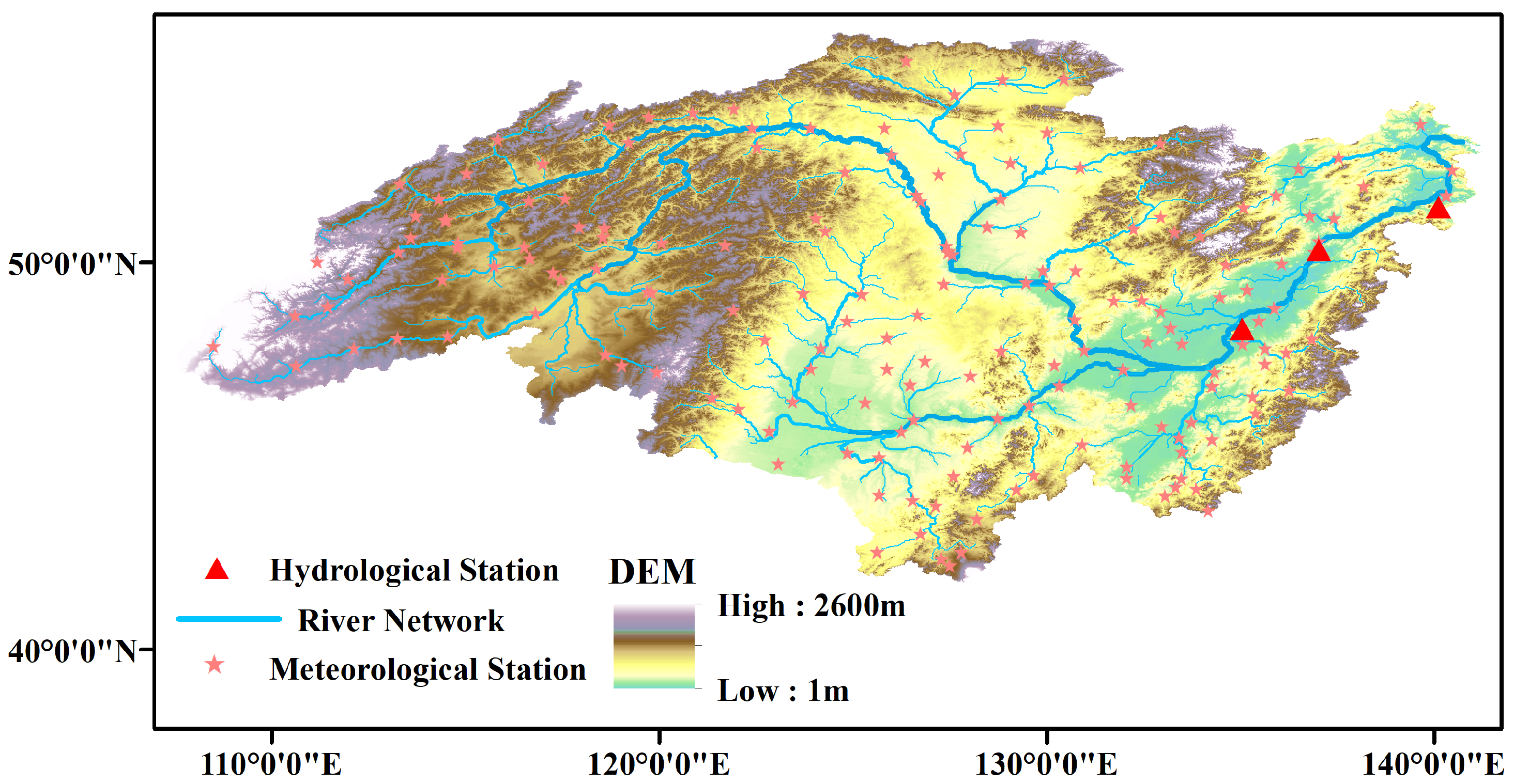
2.1. Study Area
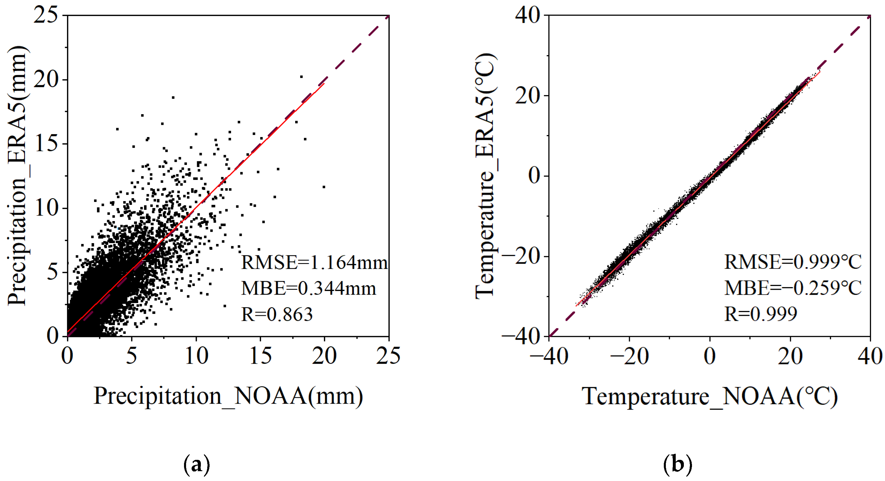
2.2. Data
2.3. Methods
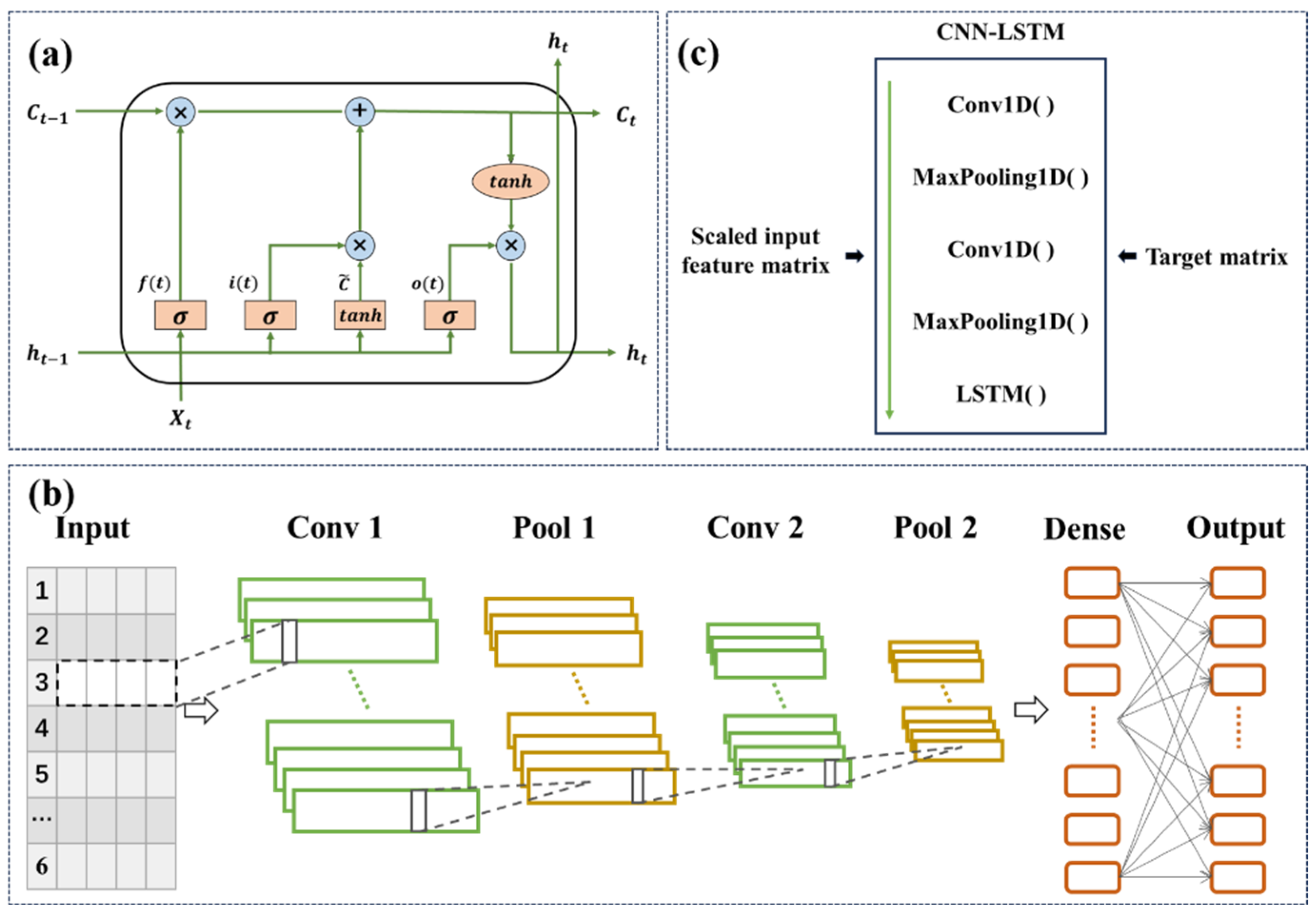
2.3.1. The Machine-Learning Models for Imputation of the Missing Data
2.3.2. Time-Series Analysis and Runoff Indicator
2.3.3. Principal Component Regression (PCR)
3. Results
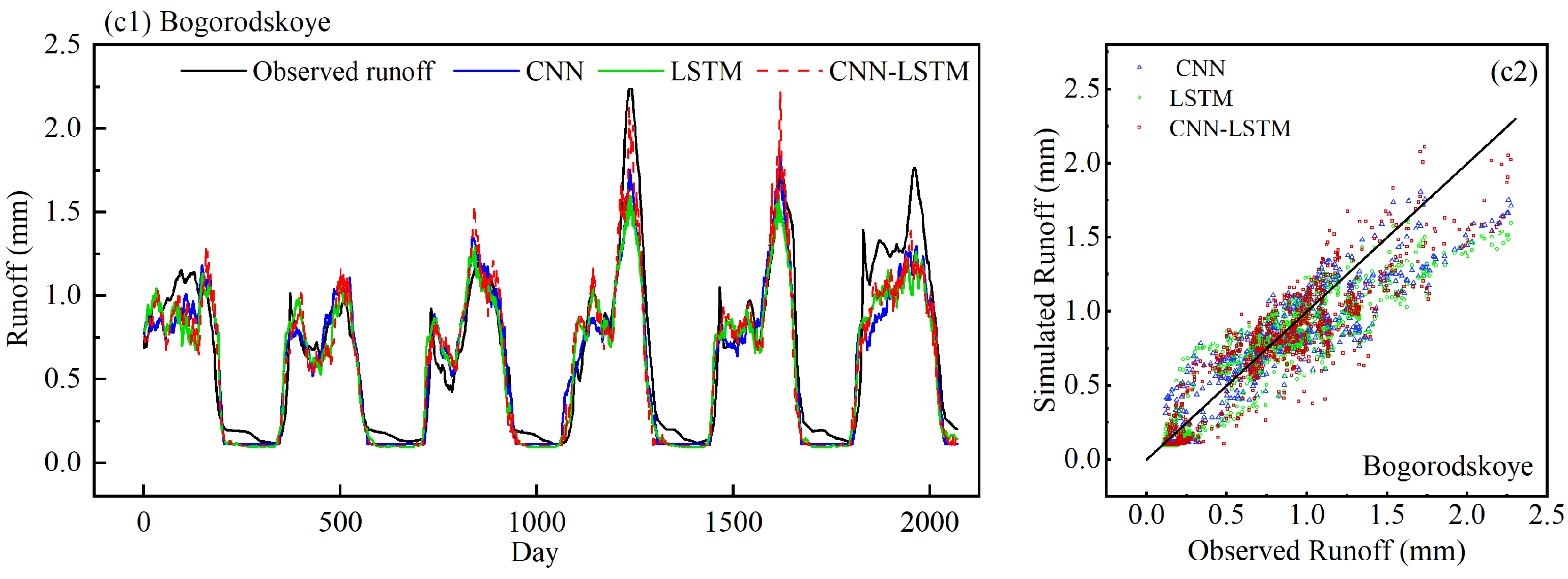
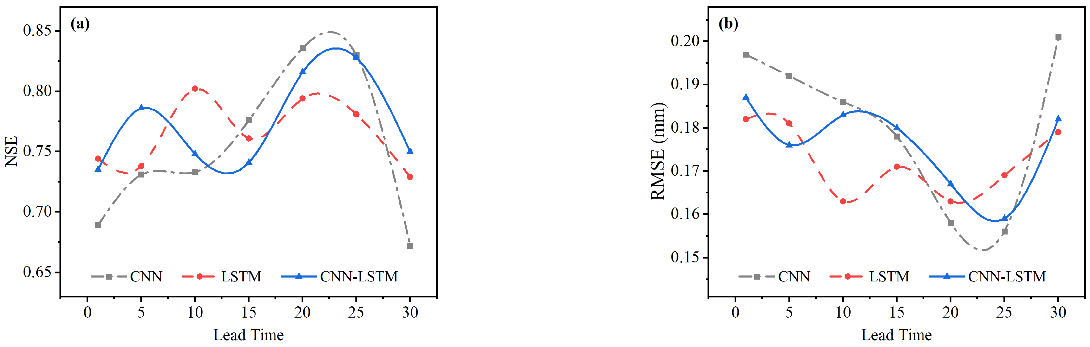
3.1. Evaluation of the Performance of Three Deep Learning Models in Daily Runoff Reconstruction
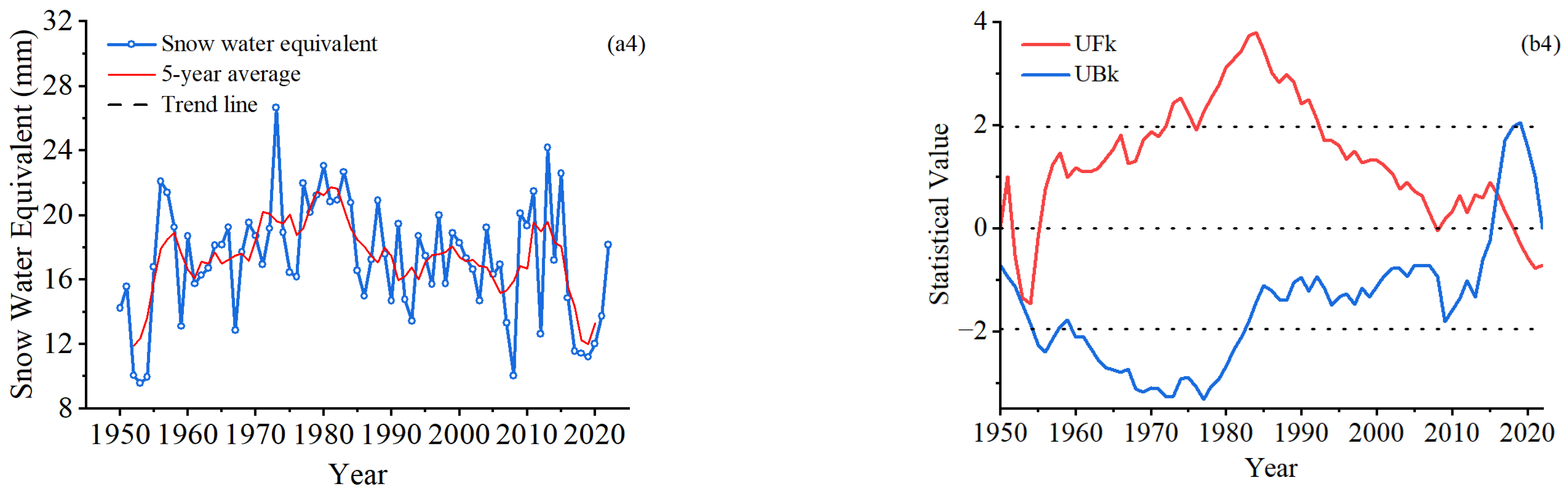
3.2. Climate Change Evidenced by Rising Air Temperatures and Increasing Precipitation and Evapotranspiration
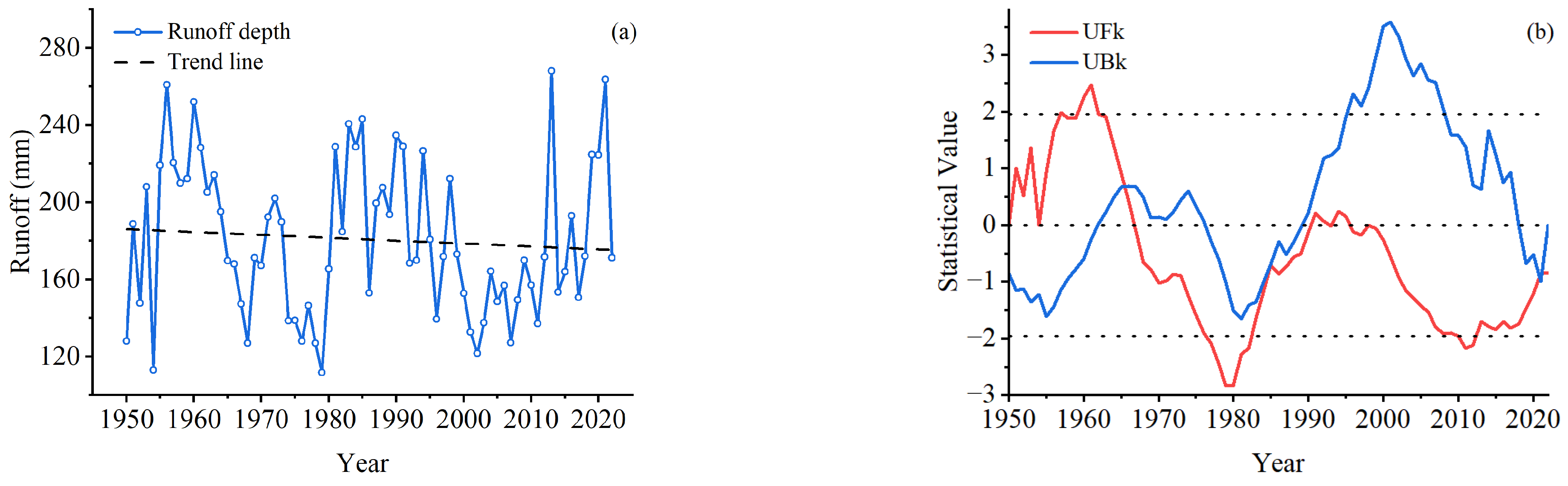
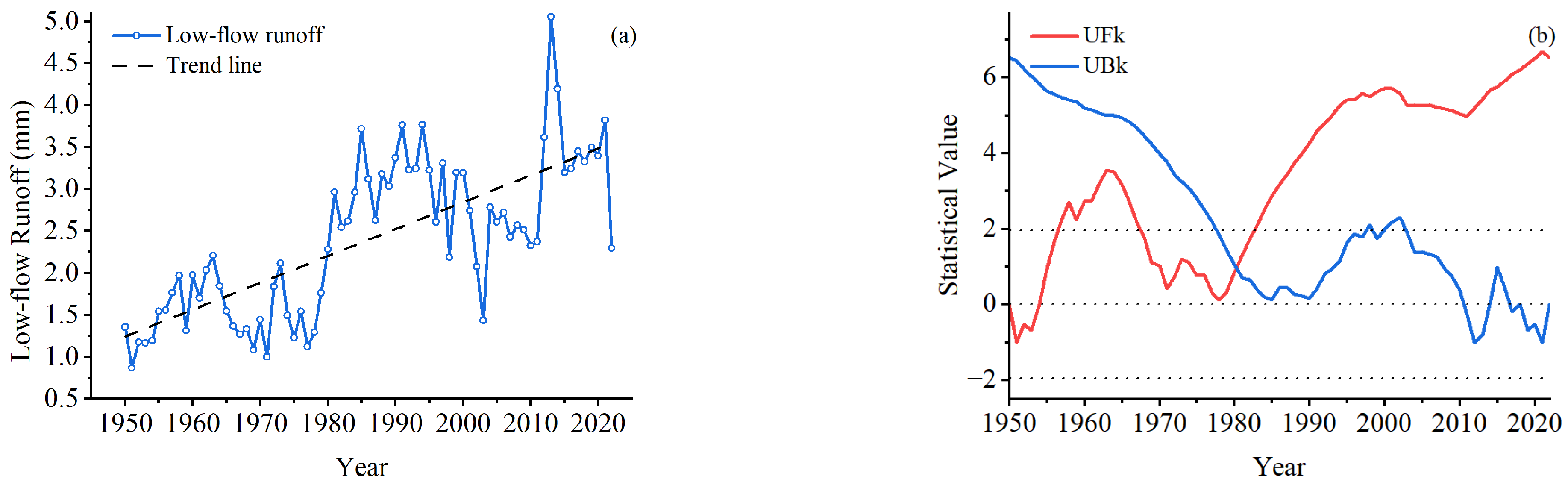
3.3. Annual Runoff and Low-Flow Runoff Exhibited Interannual Variability
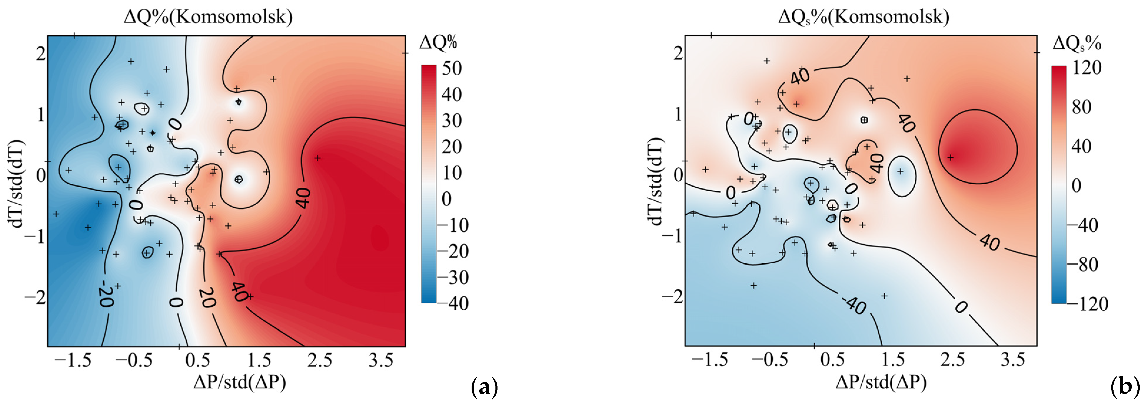
3.4. Runoff Response to Climate Change
4. Discussion
5. Conclusions
Author Contributions
Funding
Data Availability Statement
Acknowledgments
Conflicts of Interest
Appendix A
Appendix A.1

Appendix A.2

References
- Rantanen, M.; Karpechko, A.Y.; Lipponen, A.; Nordling, K.; Hyvärinen, O.; Ruosteenoja, K.; Vihma, T.; Laaksonen, A. The Arctic has warmed nearly four times faster than the globe since 1979. Commun. Earth Environ. 2022, 3, 168. [Google Scholar] [CrossRef]
- McCrystall, M.R.; Stroeve, J.; Serreze, M.; Forbes, B.C.; Screen, J.A. New climate models reveal faster and larger increases in Arctic precipitation than previously projected. Nat. Commun. 2021, 12, 6765. [Google Scholar] [CrossRef] [PubMed]
- Huang, Q.; Ma, N.; Wang, P. Faster increase in evapotranspiration in permafrost-dominated basins in the warming Pan-Arctic. J. Hydrol. 2022, 615, 128678. [Google Scholar] [CrossRef]
- Scholten, R.C.; Coumou, D.; Luo, F.; Veraverbeke, S. Early snowmelt and polar jet dynamics co-influence recent extreme Siberian fire seasons. Science 2022, 378, 1005–1009. [Google Scholar] [CrossRef]
- Biskaborn, B.K.; Smith, S.L.; Noetzli, J.; Matthes, H.; Vieira, G.; Streletskiy, D.A.; Schoeneich, P.; Romanovsky, V.E.; Lewkowicz, A.G.; Abramov, A.; et al. Permafrost is warming at a global scale. Nat. Commun. 2019, 10, 264. [Google Scholar] [CrossRef]
- Feng, D.M.; Gleason, C.J.; Lin, P.R.; Yang, X.; Pan, M.; Ishitsuka, Y. Recent changes to Arctic river discharge. Nat. Commun. 2021, 12, 6917. [Google Scholar] [CrossRef]
- Kuang, X.; Liu, J.; Scanlon, B.R.; Jiao, J.J.; Jasechko, S.; Lancia, M.; Biskaborn, B.K.; Wada, Y.; Li, H.; Zeng, Z.; et al. The changing nature of groundwater in the global water cycle. Science 2024, 383, eadf0630. [Google Scholar] [CrossRef]
- Han, J.; Liu, Z.; Woods, R.; McVicar, T.R.; Yang, D.; Wang, T.; Hou, Y.; Guo, Y.; Li, C.; Yang, Y. Streamflow seasonality in a snow-dwindling world. Nature 2024, 629, 1075–1081. [Google Scholar] [CrossRef]
- Tabari, H. Climate change impact on flood and extreme precipitation increases with water availability. Sci. Rep. 2020, 10, 13768. [Google Scholar] [CrossRef]
- Wang, K.; Zhang, T.; Yang, D. Permafrost dynamics and their hydrologic impacts over the Russian Arctic drainage basin. Adv. Clim. Change Res. 2021, 12, 482–498. [Google Scholar] [CrossRef]
- Zastruzny, S.F.; Ingeman-Nielsen, T.; Zhang, W.; Elberling, B. Accelerated permafrost thaw and increased drainage in the active layer: Responses from experimental surface alteration. Cold Reg. Sci. Technol. 2023, 212, 103899. [Google Scholar] [CrossRef]
- Song, L.; Wang, L.; Zhou, J.; Luo, D.; Li, X. Divergent runoff impacts of permafrost and seasonally frozen ground at a large river basin of Tibetan Plateau during 1960–2019. Environ. Res. Lett. 2022, 17, 124038. [Google Scholar] [CrossRef]
- Yue, Q.; Yu, G.; Miao, Y.; Zhou, Y. Analysis of Meteorological Element Variation Characteristics in the Heilongjiang (Amur) River Basin. Water 2024, 16, 521. [Google Scholar] [CrossRef]
- Novorotskii, P. Climate changes in the Amur River basin in the last 115 years. Russ. Meteorol. Hydrol. 2007, 32, 102–109. [Google Scholar] [CrossRef]
- Simonov, E.A.; Dahmer, T.D. Amur-Heilong River Basin Reader; Ecosystems Hong Kong: Hong Kong, China, 2008. [Google Scholar]
- Britannica, E. Encyclopædia Britannica; University of Chicago: Chicago, IL, USA, 1993. [Google Scholar]
- Zhong, S.; Xiyan, M.; Huang, X. Water resources exploitation and utilization of international rivers in China from the perspective of geo-security. World Reg. Stud. 2022, 31, 466. [Google Scholar]
- Gleason, C.J.; Durand, M.T. Remote sensing of river discharge: A review and a framing for the discipline. Remote Sens. 2020, 12, 1107. [Google Scholar] [CrossRef]
- Rokaya, P.; Budhathoki, S.; Lindenschmidt, K.-E. Trends in the timing and magnitude of ice-jam floods in Canada. Sci. Rep. 2018, 8, 5834. [Google Scholar] [CrossRef]
- Pavelsky, T.M.; Durand, M.T.; Andreadis, K.M.; Beighley, R.E.; Paiva, R.C.; Allen, G.H.; Miller, Z.F. Assessing the potential global extent of SWOT river discharge observations. J. Hydrol. 2014, 519, 1516–1525. [Google Scholar] [CrossRef]
- Shiklomanov, A.I.; Lammers, R.B.; Vörösmarty, C.J. Widespread decline in hydrological monitoring threatens pan-Arctic research. Eos Trans. Am. Geophys. Union 2002, 83, 13–17. [Google Scholar] [CrossRef]
- Belvederesi, C.; Zaghloul, M.S.; Achari, G.; Gupta, A.; Hassan, Q.K. Modelling river flow in cold and ungauged regions: A review of the purposes, methods, and challenges. Environ. Rev. 2022, 30, 159–173. [Google Scholar] [CrossRef]
- Xie, T.; Zhang, G.; Hou, J.; Xie, J.; Lv, M.; Liu, F. Hybrid forecasting model for non-stationary daily runoff series: A case study in the Han River Basin, China. J. Hydrol. 2019, 577, 123915. [Google Scholar] [CrossRef]
- Bhasme, P.; Bhatia, U. Improving the interpretability and predictive power of hydrological models: Applications for daily streamflow in managed and unmanaged catchments. J. Hydrol. 2024, 628, 130421. [Google Scholar] [CrossRef]
- Zhang, K.; Ma, K.; Leng, J.; He, D. Alteration in Hydrologic Regimes and Dominant Influencing Factors in the Upper Heilong-Amur River Basin across Three Decades. Sustainability 2023, 15, 10391. [Google Scholar] [CrossRef]
- Wen, K.; Gao, B.; Li, M. Quantifying the Impact of Future Climate Change on Runoff in the Amur River Basin Using a Distributed Hydrological Model and CMIP6 GCM Projections. Atmosphere 2021, 12, 1560. [Google Scholar] [CrossRef]
- Zhou, S.; Zhang, W.; Guo, Y. Impacts of climate and land-use changes on the hydrological processes in the Amur River Basin. Water 2019, 12, 76. [Google Scholar] [CrossRef]
- Zhang, K.; Li, L.; Bai, P.; Li, J.; Liu, Y. Influence of climate variability and human activities on stream flow variation in the past 50 years in Taoer River, Northeast China. J. Geogr. Sci. 2017, 27, 481–496. [Google Scholar] [CrossRef]
- Dai, C.; Li, M.; Zhang, Z. Study on hydrogeological regionalization of Heilongjiang (Amur River) Basin. Eng. J. Heilongjiang Univ. 2021, 12, 209–216. [Google Scholar] [CrossRef]
- Wu, J.; Chen, X.-Y.; Zhang, H.; Xiong, L.-D.; Lei, H.; Deng, S.-H. Hyperparameter optimization for machine learning models based on Bayesian optimization. J. Electron. Sci. Technol. 2019, 17, 26–40. [Google Scholar]
- Secci, D.; Tanda, M.G.; D’Oria, M.; Todaro, V. Artificial intelligence models to evaluate the impact of climate change on groundwater resources. J. Hydrol. 2023, 627, 130359. [Google Scholar] [CrossRef]
- Namatēvs, I. Deep convolutional neural networks: Structure, feature extraction and training. Inf. Technol. Manag. Sci. 2017, 20, 40–47. [Google Scholar] [CrossRef]
- Hochreiter, S. Long Short-term Memory. In Neural Computation; MIT-Press: Cambridge, MA, USA, 1997. [Google Scholar]
- Hochreiter, S. Untersuchungen zu dynamischen neuronalen Netzen. Diploma Tech. Univ. München 1991, 91, 31. [Google Scholar]
- Jing, X.; Luo, J.G.; Zhang, S.Y.; Wei, N. Runoff forecasting model based on variational mode decomposition and artificial neural networks. Math. Biosci. Eng. 2022, 19, 1633–1648. [Google Scholar] [CrossRef] [PubMed]
- Mann, H.B. Nonparametric tests against trend. Econom. J. Econom. Soc. 1945, 13, 245–259. [Google Scholar] [CrossRef]
- Kendall, M.G. Rank Correlation Methods; Griffin: London, UK, 1948. [Google Scholar]
- Sneyers, R. Sur L’analyse Statistique Des Séries D’observations: Note Technique N. 143; Secrétariat de l’Organisations Météorologique Mondiale: Geneva, Switzerland, 1975. [Google Scholar]
- Wang, J.; Zhang, J.; Li, Y.; Zhang, S. Variation trends of runoffs seasonal distribution of the six larger basins in China over the past 50 years. Adv. Water Sci. 2008, 19, 656–661. [Google Scholar]
- Li, L.; Hao, Z.-C.; Wang, J.-H.; Wang, Z.-H.; Yu, Z.-B. Impact of future climate change on runoff in the head region of the Yellow River. J. Hydrol. Eng. 2008, 13, 347–354. [Google Scholar] [CrossRef]
- Massy, W.F. Principal components regression in exploratory statistical research. J. Am. Stat. Assoc. 1965, 60, 234–256. [Google Scholar] [CrossRef]
- Yan, B.; Xia, Z.; Huang, F.; Guo, L.; Zhang, X. Climate change detection and annual extreme temperature analysis of the amur river basin. Adv. Meteorol. 2016, 2016, 6268938. [Google Scholar] [CrossRef]
- Tashiro, Y.; Hiyama, T.; Kanamori, H.; Kondo, M. Impact of permafrost degradation on the extreme increase of dissolved iron concentration in the Amur river during 1995–1997. Prog. Earth Planet. Sci. 2024, 11, 17. [Google Scholar] [CrossRef]
- Kurylyk, B.L.; Hayashi, M.; Quinton, W.L.; McKenzie, J.M.; Voss, C.I. Influence of vertical and lateral heat transfer on permafrost thaw, peatland landscape transition, and groundwater flow. Water Resour. Res. 2016, 52, 1286–1305. [Google Scholar] [CrossRef]
- Lamontagne-Hallé, P.; McKenzie, J.M.; Kurylyk, B.L.; Molson, J.; Lyon, L.N. Guidelines for cold-regions groundwater numerical modeling. Wiley Interdiscip. Rev. Water 2020, 7, e1467. [Google Scholar] [CrossRef]
- Sjöberg, Y.; Frampton, A.; Lyon, S.W. Using streamflow characteristics to explore permafrost thawing in northern Swedish catchments. Hydrogeol. J. 2013, 21, 121. [Google Scholar] [CrossRef]
- Zhou, J.; Mao, W.; Jiao, M.; An, M.; Shen, Y. The responses of the runoff processes to climate change in the Qingshuihe River watershed on the southern slope of Tianshan Mountains. J. Glaciol. Geocryol. 2014, 36, 685–690. [Google Scholar]
- Risbey, J.S.; Entekhabi, D. Observed Sacramento Basin streamflow response to precipitation and temperature changes and its relevance to climate impact studies. J. Hydrol. 1996, 184, 209–223. [Google Scholar] [CrossRef]
- Wang, P.; Huang, Q.; Pozdniakov, S.P.; Liu, S.; Ma, N.; Wang, T.; Zhang, Y.; Yu, J.; Xie, J.; Fu, G. Potential role of permafrost thaw on increasing Siberian river discharge. Environ. Res. Lett. 2021, 16, 034046. [Google Scholar] [CrossRef]
- Wang, P.; Huang, Q.; Liu, S.; Cai, H.; Yu, J.; Wang, T.; Chen, X.; Pozdniakov, S.P. Recent regional warming across the Siberian lowlands: A comparison between permafrost and non-permafrost areas. Environ. Res. Lett. 2022, 17, 054047. [Google Scholar] [CrossRef]
- Wang, P.; Huang, Q.; Tang, Q.; Chen, X.; Yu, J.; Pozdniakov, S.P.; Wang, T. Increasing annual and extreme precipitation in permafrost-dominated Siberia during 1959–2018. J. Hydrol. 2021, 603, 126865. [Google Scholar] [CrossRef]
- Krylova, A.I.; Lapteva, N.A. Modeling Long-Term Dynamics of River Flow in the Lena River Basin Based on a Distributed Conceptual Runoff Model. Water Resour. 2024, 51, 393–404. [Google Scholar] [CrossRef]
- Debolskiy, M.V.; Alexeev, V.A.; Hock, R.; Lammers, R.B.; Shiklomanov, A.; Schulla, J.; Nicolsky, D.; Romanovsky, V.E.; Prusevich, A. Water balance response of permafrost-affected watersheds to changes in air temperatures. Environ. Res. Lett. 2021, 16, 084054. [Google Scholar] [CrossRef]
- Makarieva, O.; Nesterova, N.; Post, D.A.; Sherstyukov, A.; Lebedeva, L. Warming temperatures are impacting the hydrometeorological regime of Russian rivers in the zone of continuous permafrost. Cryosphere 2019, 13, 1635–1659. [Google Scholar] [CrossRef]
- Tananaev, N.I.; Makarieva, O.M.; Lebedeva, L.S. Trends in annual and extreme flows in the Lena River basin, Northern Eurasia. Geophys. Res. Lett. 2016, 43, 10764–10772. [Google Scholar] [CrossRef]
- Qin, J.; Ding, Y.; Han, T. Quantitative assessment of winter baseflow variations and their causes in Eurasia over the past 100 years. Cold Reg. Sci. Technol. 2020, 2020, 102989. [Google Scholar] [CrossRef]
- Teutschbein, C.; Grabs, T.; Karlsen, R.H.; Laudon, H.; Bishop, K. Hydrological response to changing climate conditions: Spatial streamflow variability in the boreal region. Water Resour. Res. 2015, 51, 9425–9446. [Google Scholar] [CrossRef]
- Dethier, E.N.; Sartain, S.L.; Renshaw, C.E.; Magilligan, F.J. Spatially coherent regional changes in seasonal extreme streamflow events in the United States and Canada since 1950. Sci. Adv. 2020, 6, eaba5939. [Google Scholar] [CrossRef] [PubMed]
- Blöschl, G.; Hall, J.; Viglione, A.; Perdigão, R.A.; Parajka, J.; Merz, B.; Lun, D.; Arheimer, B.; Aronica, G.T.; Bilibashi, A. Changing climate both increases and decreases European river floods. Nature 2019, 573, 108–111. [Google Scholar] [CrossRef]
- Wang, H.; Liu, J.; Klaar, M.; Chen, A.; Gudmundsson, L.; Holden, J. Anthropogenic climate change has influenced global river flow seasonality. Science 2024, 383, 1009–1014. [Google Scholar] [CrossRef]
- Sjöberg, Y.; Jan, A.; Painter, S.L.; Coon, E.T.; Carey, M.P.; O’Donnell, J.A.; Koch, J.C. Permafrost Promotes Shallow Groundwater Flow and Warmer Headwater Streams. Water Resour. Res. 2021, 57, e2020WR027463. [Google Scholar] [CrossRef]
- Diak, M.; Böttcher, M.E.; Ehlert von Ahn, C.M.; Hong, W.-L.; Kędra, M.; Kotwicki, L.; Koziorowska-Makuch, K.; Kuliński, K.; Lepland, A.; Makuch, P.; et al. Permafrost and groundwater interaction: Current state and future perspective. Front. Earth Sci. 2023, 11, 1254309. [Google Scholar] [CrossRef]
- Walvoord, M.A.; Striegl, R.G. Increased groundwater to stream discharge from permafrost thawing in the Yukon River basin: Potential impacts on lateral export of carbon and nitrogen. Geophys. Res. Lett. 2007, 34. [Google Scholar] [CrossRef]
- Kurylyk, B.L.; Walvoord, M.A. Permafrost hydrogeology. In Arctic Hydrology, Permafrost and Ecosystems; Springer: Berlin/Heidelberg, Germany, 2021; pp. 493–523. [Google Scholar]
- Song, C.; Wang, G.; Sun, X.; Hu, Z. River runoff components change variably and respond differently to climate change in the Eurasian Arctic and Qinghai-Tibet Plateau permafrost regions. J. Hydrol. 2021, 601, 126653. [Google Scholar] [CrossRef]
- Walvoord, M.A.; Kurylyk, B.L. Hydrologic impacts of thawing permafrost—A review. Vadose Zone J. 2016, 15, vzj2016. [Google Scholar] [CrossRef]
- Ala-Aho, P.; Soulsby, C.; Pokrovsky, O.; Kirpotin, S.; Karlsson, J.; Serikova, S.; Vorobyev, S.; Manasypov, R.; Loiko, S.; Tetzlaff, D. Using stable isotopes to assess surface water source dynamics and hydrological connectivity in a high-latitude wetland and permafrost influenced landscape. J. Hydrol. 2018, 556, 279–293. [Google Scholar] [CrossRef]
- Park, H.; Kim, Y.; Kimball, J.S. Widespread permafrost vulnerability and soil active layer increases over the high northern latitudes inferred from satellite remote sensing and process model assessments. Remote Sens. Environ. 2016, 175, 349–358. [Google Scholar] [CrossRef]
- Shan, W.; Wang, Y.; Guo, Y.; Zhang, C.; Liu, S.; Qiu, L. Impacts of climate change on permafrost and hydrological processes in Northeast China. Sustainability 2023, 15, 4974. [Google Scholar] [CrossRef]
- Connon, R.F.; Quinton, W.L.; Craig, J.R.; Hayashi, M. Changing hydrologic connectivity due to permafrost thaw in the lower Liard River valley, NWT, Canada. Hydrol. Process. 2014, 28, 4163–4178. [Google Scholar] [CrossRef]
- Obu, J.; Westermann, S.; Bartsch, A.; Berdnikov, N.; Christiansen, H.H.; Dashtseren, A.; Delaloye, R.; Elberling, B.; Etzelmüller, B.; Kholodov, A.; et al. Northern Hemisphere permafrost map based on TTOP modelling for 2000–2016 at 1 km2 scale. Earth-Sci. Rev. 2019, 193, 299–316. [Google Scholar] [CrossRef]
- Qin, J.; Ding, Y.; Shi, F.; Cui, J.; Chang, Y.; Han, T.; Zhao, Q. Links between seasonal suprapermafrost groundwater, the hydrothermal change of the active layer, and river runoff in alpine permafrost watersheds. Hydrol. Earth Syst. Sci. 2024, 28, 973–987. [Google Scholar] [CrossRef]


| Model | Hydrological Station | RMSE (mm) | MAE (mm) | NSE | R |
|---|---|---|---|---|---|
| Komsomolsk | 0.16 | 0.12 | 0.84 | 0.94 | |
| CNN | Khabarovsk | 0.16 | 0.12 | 0.80 | 0.93 |
| Bogorodskoye | 0.18 | 0.13 | 0.83 | 0.94 | |
| Komsomolsk | 0.16 | 0.11 | 0.79 | 0.94 | |
| LSTM | Khabarovsk | 0.15 | 0.11 | 0.80 | 0.94 |
| Bogorodskoye | 0.19 | 0.13 | 0.78 | 0.93 | |
| Komsomolsk | 0.17 | 0.12 | 0.82 | 0.93 | |
| CNN-LSTM | Khabarovsk | 0.18 | 0.13 | 0.76 | 0.91 |
| Bogorodskoye | 0.18 | 0.13 | 0.84 | 0.93 |
| P | T | ET | SWE | |||||||||
|---|---|---|---|---|---|---|---|---|---|---|---|---|
| Trend | Z | Slope (mm/a) | Trend | Z | Slope (°C/a) | Trend | Z | Slope (mm/a) | Trend | Z | Slope (mm/a) | |
| Spring | no | 0.615 | 0.003 | upward | 5.291 | 0.052 | upward | 3.834 | 0.035 | no | −0.824 | −0.035 |
| Summer | no | 1.390 | 0.123 | upward | 5.929 | 0.022 | no | 1.824 | 0.031 | no | −1.548 | −0.014 |
| Autumn | no | −0.655 | −0.021 | upward | 3.700 | 0.016 | no | 0.929 | 0.010 | no | −1.538 | −0.005 |
| Winter | upward | 2.462 | 0.037 | upward | 4.786 | 0.046 | upward | 3.672 | 0.002 | no | 0.052 | 0.007 |
| Index (k) | 1 | 2 | 3 | 4 | 5 |
|---|---|---|---|---|---|
| Komsomolsk | 1.000 | 2.230 | 11.592 | 20.018 | 82.948 |
| Khabarovsk | 1.000 | 2.511 | 11.550 | 19.393 | 80.445 |
| Bogorodskoye | 1.000 | 2.288 | 11.644 | 20.468 | 84.052 |
| Hydrological Station | ||||||
|---|---|---|---|---|---|---|
| Komsomolsk | 0.484 | 1.647 | −0.058 | 1.437 | 0.838 | |
| Khabarovsk | 18.107 | 0.457 | 3.361 | −0.042 | 1.768 | 0.839 |
| Bogorodskoye | 55.848 | 0.415 | 3.156 | −0.037 | 0.561 | 0.811 |
| Hydrological Station | |||||
|---|---|---|---|---|---|
| Komsomolsk | 0.736 | 0.04 | −0.244 | 0.122 | 0.838 |
| Khabarovsk | 0.776 | −0.045 | −0.337 | 0.139 | 0.809 |
| Bogorodskoye | 0.710 | 0.088 | −0.178 | 0.058 | 0.769 |
Disclaimer/Publisher’s Note: The statements, opinions and data contained in all publications are solely those of the individual author(s) and contributor(s) and not of MDPI and/or the editor(s). MDPI and/or the editor(s) disclaim responsibility for any injury to people or property resulting from any ideas, methods, instructions or products referred to in the content. |
© 2025 by the authors. Licensee MDPI, Basel, Switzerland. This article is an open access article distributed under the terms and conditions of the Creative Commons Attribution (CC BY) license (https://creativecommons.org/licenses/by/4.0/).
Share and Cite
Li, J.; Wang, R.; Huang, Q.; Xia, J.; Wang, P.; Fang, Y.; Shamov, V.V.; Frolova, N.L.; She, D. Climate Warming-Induced Hydrological Regime Shifts in Cold Northeast Asia: Insights from the Heilongjiang-Amur River Basin. Land 2025, 14, 980. https://doi.org/10.3390/land14050980
Li J, Wang R, Huang Q, Xia J, Wang P, Fang Y, Shamov VV, Frolova NL, She D. Climate Warming-Induced Hydrological Regime Shifts in Cold Northeast Asia: Insights from the Heilongjiang-Amur River Basin. Land. 2025; 14(5):980. https://doi.org/10.3390/land14050980
Chicago/Turabian StyleLi, Jiaoyang, Ruixin Wang, Qiwei Huang, Jun Xia, Ping Wang, Yuanhao Fang, Vladimir V. Shamov, Natalia L. Frolova, and Dunxian She. 2025. "Climate Warming-Induced Hydrological Regime Shifts in Cold Northeast Asia: Insights from the Heilongjiang-Amur River Basin" Land 14, no. 5: 980. https://doi.org/10.3390/land14050980
APA StyleLi, J., Wang, R., Huang, Q., Xia, J., Wang, P., Fang, Y., Shamov, V. V., Frolova, N. L., & She, D. (2025). Climate Warming-Induced Hydrological Regime Shifts in Cold Northeast Asia: Insights from the Heilongjiang-Amur River Basin. Land, 14(5), 980. https://doi.org/10.3390/land14050980