Time Allocation Effect: How Does the Combined Adoption of Conservation Agriculture Technologies Affect Income?

Abstract

The adoption of conservation agriculture techniques plays a crucial role in preventing soil erosion and guaranteeing food security. The purpose of this paper is to examine the impact of the adoption of conservation agricultural technologies on income. Based on the survey data of 922 households in five provinces and cities in the Bohai Rim region in 2023, the study analyzes the impact of different attributes of technology adoption on farm household income through ESR (endogenous switching regression) models and different forms of mediated effects models. The empirical results show the following: (1) The income effects generated by different adoption statuses of conservation agriculture (CA) technologies vary, and the income effects for farmers who adopt multiple conservation agriculture (CA) technologies jointly are even worse. (2) Farmers’ time allocation mediates the effects of technology attributes on adoption. Specifically, farm work is the main mediating variable, while off-farm work plays a moderating role between the yield effect and income. (3) The complex technology adoption chain inhibits farmers from increasing production and income, while the farmers’ jobs in the non-agricultural sector have reduced this impact to a certain extent. In terms of policy recommendations, governments should enhance technical training programs for farmers, improve the market environment, and offer access to highly mechanized agricultural production trusteeship services to encourage the greater adoption of conservation agriculture (CA) technology among farmers.

1. Introduction

Most studies agree that conservation tillage technology adoption can reduce production costs and improve economic returns [1,2]. Since conservation agriculture (CA) technology was first developed in the 1960s, countries worldwide have promoted it to improve the arable land quality, with several related policies. In numerous developing nations, the uptake of conservation tillage technology is facilitated by agricultural enterprises [3,4], industry associations [5], and government departments through publicity, training, and guidance [6,7,8]. Various initiatives promoting conservation tillage technology have been implemented in many developing countries, including China [9]. However, according to conservation tillage technology promotion data from China’s Ministry of Agriculture and Rural Development (MARD), as of 2020, the area of China’s CA technology implementation only accounted for 6.13% of the country’s total cropland area. In addition, the area of China’s conservation tillage application experienced a rapid decline from 2015 to 2020, which means that a portion of farmers withdrew from adopting conservation tillage technology. As we know, CA technology differs from traditional farming techniques and can be categorized into deep topsoil loosening, straw return to the field, no-tillage of stubble, and green insect and weed control [10,11]. The existence of multiple technologies provides a way for us to discuss the revenue-increasing effect of CA technologies from the perspective of adopting multiple CA technologies simultaneously.

Currently, research on conservation tillage technology adoption focuses on the factors that influence farmers’ adoption of CA technology [12]. However, less attention has been paid to the adoption effect of conservation tillage techniques by farmers. In addition to considering input costs and profitability, farmers are also influenced by their education level, risk preference, social network and information access when adopting CA technology [13,14]. Apart from personal factors, CA technology requires inputs from specialized farm equipment and the effective joint adoption of technologies to ensure better yield output. Otherwise, incorrect agronomic practices may reduce crop yields [15]. From a technical standpoint, the adoption of CA technologies—such as no-tillage, straw returning, and subsoiling—necessitates that farmers adjust to the demands of agricultural production and CA technical requirements, which include minimizing soil disturbance, implementing water-saving irrigation, and managing fertilizer input. The integration of these conservation tillage techniques results in varied input levels and combinations of production factors, altering their allocation efficiency and affecting crop yield and income [16,17]. Yield and income effects are crucial for assessing the impact of technology adoption. The existing literature has examined the impact of CA technology adoption on farmers’ incomes in Africa, as well as the underlying mechanisms driving the economic outcomes of CA practices. The findings indicate that improvements in crop diversification [16], soil quality [18], and cost-saving inputs [19] are key determinants of the economic effectiveness of CA. Additionally, research has suggested that the income effects of CA technology may vary with the level of farmer poverty [20]. However, the existing scholarship has not addressed the perspectives of technology adoption combinations or the labor sector transitions of farmers. This study provides marginal contributions to the literature in several aspects: First, to the best of our knowledge, this is the first time that the income effects of adopting different conservation tillage technologies have been discussed using micro-level data from regional representatives in China, and the significance of this discussion lies in the fact that China’s urban–rural dual structure makes the transfer of farmers between labor sectors more prominent [21], which provides a possible reasonable explanation for the large-scale withdrawal of farmers from the technology adoption team. Second, this study fills the gap in the current literature on the mechanisms of technology adoption and farmers’ incomes by discussing the impact of different time allocations on income. Third, the income effect of time allocation is tested using an endogenous conversion model and a variety of mediating effect models, and a series of robustness tests are conducted to strengthen the reliability of the conclusions.

The remainder of the paper is structured as follows. Section 2 presents the analytical framework based on a review of the literature on the relationship between technology attributes and farmers’ time reallocation and income. Section 3 presents the data and methodology used to study the interaction between technology attributes and the time allocation of the income in farm households. Section 4 presents the empirical analysis and conclusions. Section 5 presents the conclusions and policy recommendations.

2. Literature Review and Theoretical Hypotheses

Abundant research has been conducted on farmers’ decision-making and time allocation behavior. Becker (1965) [22] proposed a time allocation theory based on Mincer’s (1962) [23] theory of women’s time trade-off between housework and paid work, arguing that farmers maximize household labor utility by adjusting the allocation of their time under the constraints of income, production function, and consumption. Developmental economists proposed the equilibrium condition of production and consumption time for farm households, which is that the marginal effect of production is equal to that of leisure in the household model, suggesting that this equilibrium condition may exist for farm households [24]. Several studies have demonstrated the effects of time allocation on income in farm households, incorporating factors such as gender and age [25,26]. However, the relationship between technology attributes and farm household income has not been studied from the household time allocation perspective. Time is a limited resource that farmers can only allocate in a flow among the agricultural sector, labor market, household labor, and leisure [27]. Given the contradiction between the dependence of CA technology on machinery and labor supply, we attempt to explore previous studies on farmers’ time allocation [28,29], without considering leisure and consumption. In this study, we define time allocation in farm households as being classified into crop cultivation, non-farm labor, and hired labor, where crop cultivation time and hired labor time are farmers’ time allocation to agricultural activities.

2.1. Technical Attributes and Farm Household Revenue

The problem of adopting technologies with different attributes necessitates an examination of the effects of technology adoption. Specifically, the question of whether the adoption of agricultural technology promotes farm households’ income growth has been a controversial topic in academia. Cochrane (1958) noted in his “agricultural technology treadmill hypothesis” that producers who adopt technology first increase their labor productivity, thus reducing the unit production cost of products and earning more income [30]. However, technological progress in the agricultural sector changes the supply side, leading to most adopted technologies having insignificant income-generating effects. Based on this, Hayami and Herdt (1977) proposed that consumers capture most of the welfare that technology adoption generates, and that the long-run equilibrium of the income-raising effect on farm households is weak [31]. By contrast, Schultz (1966) introduced the concept of human capital investment within the income stream price model [32]. He believed that this investment could increase income by stimulating farmers to adopt agricultural technologies. Empirical studies also differ on whether CA technology adoption improves farmers’ incomes. Some scholars argue that it significantly improves farmers’ incomes by increasing crop yields [33,34], whereas others posit that farmers’ incomes could decrease instead [35], particularly because of the reduced crop yields that may result from adopting multiple CA technologies [36], which can lead to a loss of farmers’ income. In China’s Loess Plateau, CA technology has improved soil water use efficiency and crop yield, while boosting soil productivity and farmers’ income [37,38]. Similarly, in South Asia, the adaptation of CA technology to local cropping systems has indirectly influenced farmers’ economic gains [39]. The above literature suggests that adopting different CA technologies or combinations of them may have differential effects on farmers’ income. Therefore, we propose the following hypothesis:

H1: 

The revenue effects of adopting CA technologies or combinations of CA technologies with different attributes may differ.

2.2. Technical Attributes and Time Allocation

Farmers’ adoption of new technologies and their household time allocation are strongly linked, with farmers adopting technologies based on optimizing their time allocation [40]. Farmers rationally set their household schedules, and their attitudes toward adopting improved technologies are based on considerations of household time allocation. Technology is an exogenous variable, and its uptake and use directly affect the agricultural activity of household time allocation, disrupting the dynamic time allocation equilibrium between the agricultural sector and other sectors [41].

Thus, adopting single or combined agricultural technologies may affect farmers’ time allocation. In the limited research on CA technology adoption and time allocation, some scholars have demonstrated that adopting CA technologies can effectively reduce farmers’ labor requirements and the time spent on labor in the agricultural sector [42,43,44]. However, not all CA technologies can help farmers reduce labor input in field management activities, and other scholars have reached the opposite conclusion. Although conservation tillage can improve soil health and long-term yields, straw returning is accompanied by increased labor intensity due to crop residue management, biomass accumulation, and mulch maintenance, which significantly increases the time input for manual management [45,46]. Especially in areas with low mechanization levels, after farmers adopt CA, the frequency and complexity of field management activities actually increase [47].

H2: 

Adoption of CA technologies with different attributes may affect farmers’ time allocation.

2.3. Time Allocation and Farm Household Revenue

A model suggests that individuals’ time spent on household production and market activity depends on wage rates, household productivity, and substitution rates between sectors. Studies have shown that household income influences intra-household time allocation, affecting how much labor farm households supply to different sectors [48,49,50,51,52], but research on how intra-household time allocation impacts farm household income remains limited. Rosales-Salas and Jara-Díaz revised the time allocation model to account for the value of leisure and the use of hired labor, which previous models had overlooked [29]. They argued that farm households also need to consider non-farm production and hiring labor [53], especially when farm operators lack the skills to operate advanced machinery [54]. Research by Charlton and Kostandini supports this, showing that big farm operators may increase their non-farm labor supply (i.e., hiring) in response to yield fluctuations caused by skill shortages [55]. Diverse constraints and preferences among household members lead farmers to engage more in profitable non-farm activities to mitigate income risks [56]. Apart from this, higher education levels can increase wage rates in the non-farm sector, encouraging farmers to invest more time in non-farm work [57,58], which may indirectly affect how they schedule their crop cultivation time. In addition, improved agricultural technology enhances productivity, prompting farmers to expand farmland operations and adjust their time allocation between farming and non-farming activities as dynamic additions [59,60,61].

The above analysis suggests that the corresponding time input of hired labor and non-farm labor time will result in farmers changing the demand for inputs of crop planting time, producing a moderating effect. However, such an effect may not necessarily be effective for large-scale farmers with planting experience. Thus, the relationship between employment hours and off-farm work and crop scheduling can either be parallel or moderated by changes in the characteristics of the target population and realities of the situation. Based on the comparative discussion of the literature, this paper constructs a theoretical framework for the impact of CA technology adoption on farmers’ income, as shown in Figure 1. Therefore, we propose the following hypotheses:

H3a: 

The three types of time allocation for farmers have parallel mediating effects in the adoption of CA technology in the process of its impact on farm income.

H3b: 

Only crop planting schedules mediate the impact of CA technology adoption on farm incomes, while hired and off-farm labor time moderates crop planting schedules.

3. Research Methodology and Data Sources

3.1. Research Methodology

3.1.1. Recognition of CA

To determine whether the adoption of different types of CA technologies affects income, it is first necessary to identify the specific manifestations of the technical attributes of CA in terms of machinery use, field management, and time input. According to the specialization of CA technology production machinery and biochemical mechanisms of the soil, the effect of farmers’ food cultivation on the production chain is divided into the following three types in comparison with the traditional cultivation chain:

(1) Stubble-free (less) tillage technology: this eliminates the need for plowing, rotary tillage, and soil turning to allow farmers to save the operational inputs of the mechanized plowing process, reduce the number of operational links, and save labor and time inputs;

(2) Straw (mulching, crushing) field return technology: straw crushing, baling, and burning are eliminated, reducing farmers’ straw treatment inputs after harvesting each crop. The number of operation links is also reduced, saving labor and time inputs; however, straw mulching may lead to an increase in pests and weeds, which will increase the complexity of farmers’ field management and extend their time input in the agricultural sector;

(3) Deep topsoil loosening technology: this works directly on crushing the subsoil layer of the land (30 cm), but only completes the deep opening of ridges or furrows. After the deep loosening of the topsoil, rotary plows or other soil-turning machinery are needed to further crush the crusted surface layer. This link increases the rotary plowing and soil-turning links, and farmers will increase mechanized plowing before sowing after using this technology, significantly increasing the number of operation links and input of labor and time.

Simultaneously considering the identification of the three attributes of technology adoption is cumbersome, and the above technologies are not mutually independent of each other. When farmers are superimposed on the use of the above technologies, then the production chain may also be due to the hedging on the technological chain without change, and does not produce an increase or decrease in time and labor. To simplify the identification of the different attributes of the farmers of the state of the technology, adopt the specific calculation of the idea of the different attributes of the state of the technology as follows.

First, an increase in the number of links after adopting deep-polishing technology is recorded as 1, whereas a non-increase without adopting this technology is recorded as 0. Second, a decrease in the number of links after adopting no-tillage and straw-returning technology is recorded as 1, whereas a non-decrease without adopting this technology is recorded as 0. Third, based on the definition of the complexity of technological attributes by Rogers (2008) [62], a non-change in the number of links after the superimposed adoption of both of these technologies is recorded as 1 (i.e., composite-type technology adoption), whereas a change without the superimposed adoption of these technologies is recorded as 0 (i.e., mono-type technology adoption), which is uniformly abbreviated as such below.

A simultaneous decision-making problem may exist between farmers making technology adoption decisions and their income, and collecting data on two different technology-adoption statuses of the same farmer simultaneously is impossible. Meanwhile, the decision to adopt agricultural technology is not a random process, but rather influenced by unobservable factors. Directly comparing the incomes of adopters and non-adopters can lead to endogeneity bias in the estimation results. The endogenous switching regression (ESR) model addresses this issue by establishing a selection equation and outcome equations under different adoption states. Importantly, ESR not only estimates the actual income, but also the counterfactual “what-if” income, providing a more accurate assessment of the reality. Thus, this study uses an ESR model for the analysis, estimating the choice and outcome Equations (1)–(3) separately:

$$D_i=\phi Z_i+v_i,D_i=1(D_i^{*}>0)$$

(1)

$$Y_{1i}={\beta }_{i1}{X}_i+{\epsilon }_{1i},D_i=1$$

(2)

$$Y_{0i}={\beta }_{i0}{X}_i+{\epsilon }_{0i},D_i=0$$

(3)

where ${\mathrm{Y}}_{\mathrm{i}}$ denotes total farm household income, ${\mathrm{X}}_{\mathrm{i}}$ is a vector of variables affecting CA technology adoption, ${\mathrm{D}}_{\mathrm{i}}$ denotes the two different states of CA technology adoption (${\mathrm{D}}_{\mathrm{i}}=1$ for composite technology and ${\mathrm{D}}_{\mathrm{i}}=0$ for mono technology), $\beta$ and $\phi$ are vectors of the parameters to be estimated, and ${\epsilon }_i,$ and $v_i$ are independently and identically distributed error terms. Farmers’ net income expectation after adopting technology ($D_i\mathrm{*}$) is unobserved; therefore, it must be re-fitted using the estimation of observable variables such as personal and household characteristics to continue the identification, in which the identification condition is to include at least one variable different from ${\mathrm{C}}_{\mathrm{i}}$ as an instrumental variable, for which “the number of times that farmers have been trained” is chosen in this study. The existing literature has indicated that the number of times farmers participate in agricultural technology extension service training can influence technology adoption, and that it only affects income through technology adoption. Meanwhile, it meets both the relevance and exogeneity assumptions, providing strong support for using the number of training sessions as an instrumental variable [63]. Equation (1) is the behavioral equation for technology adoption decisions, and Equations (2) and (3) are the outcome equations for estimating technology adoption. The ESR model introduces the possible problem of unobserved data into the outcome equations by using the inverse Mills ratios (λ) computed in Equation (1). Specifically, after computing the inverse Mills ratios, ${\mathsf{\lambda }}_{\mathrm{i}1},{\mathsf{\lambda }}_{\mathrm{i}0}$, controlling for selective bias due to the unobserved variables, as well as the error term’s covariance ${\mathsf{\sigma }}_{\mathsf{\mu }1}=\mathrm{cov}\left({\mathsf{\mu }}_{\mathrm{i}},{\mathsf{\epsilon }}_{\mathrm{i}1}\right),{\mathsf{\sigma }}_{\mathsf{\mu }0}=\mathrm{c}\mathrm{o}\mathrm{v}({\mathsf{\mu }}_{\mathrm{i}},{\mathsf{\epsilon }}_{\mathrm{i}0})$, and subsequently bringing all four into Equations (2) and (3), Equations (4) and (5) are obtained as follows:

$$Y_{i1}={\beta }_{i1}{X}_i+{\sigma }_{\mu 1}{\lambda }_{i1}+{\zeta }_{i1} \mathit{if} D_i=1$$

(4)

$$Y_{i0}={\beta }_{i0}{X}_i+{\sigma }_{\mu 0}{\lambda }_{i0}+{\zeta }_{i0} if D_i=0$$

(5)

where ${\mathsf{\zeta }}_{\mathrm{i}1},{\mathsf{\zeta }}_{\mathrm{i}0}$ satisfy the null mean assumption. In addition, ${\mathsf{\rho }}_{\mathsf{\mu }1} \mathrm{and} {\mathsf{\rho }}_{\mathsf{\mu }0}$ denote the correlation coefficients of the covariance of the behavioral and outcome equations, respectively, and if the coefficients are significant, it indicates selection bias caused by unobserved factors. Based on previous computations, the average treatment effect of different technology attributes is estimated further by comparing the farm income expectations of different technology attributes adopted in factual and counterfactual scenarios.

Income expectations of farmers who have adopted composite technologies:

$$E[Y_{i1}\mid D_i=1]={{\beta }^{\prime }}_{i1}{X}_{i1}+{\sigma }_{\mu 1}{\lambda }_{i1}$$

(6)

Income expectations of farmers who have adopted monotypic technologies:

$$E[Y_{i0}\mid D_i=0]={{\beta }^{\prime }}_{i0}{X}_{i0}+{\sigma }_{\mu 0}{\lambda }_{i0}$$

(7)

Income expectations of farmers who have adopted composite technology in a non-composite technology scenario:

$$E[Y_{i0}\mid D_i=1]={{\beta }^{\prime }}_{i0}{X}_{i1}+{\sigma }_{\mu 0}{\lambda }_{i1}$$

(8)

Income expectations of farmers who have adopted mono-type technologies in the absence of mono-type technologies:

$$E[Y_{i1}\mid D_i=0]={{\beta }^{\prime }}_{i1}{X}_{i0}+{\sigma }_{\mu 1}{\lambda }_{i0}$$

(9)

Through Equations (6) and (8), the income effect of farmers adopting composite-type technology is obtained:

$$ATT=E\left[Y_{i1}∣D_i=1\right]-E\left[Y_{i0}∣D_i=1\right]=({{\beta }^{\prime }}_{i1}-{\beta }_{i0}^{\prime })X_{i1}+({\sigma }_{\mu 1}-{\sigma }_{\mu 0}){\lambda }_{i1}$$

(10)

Through Equations (7) and (9), the income effect of farmers adopting a single type of technology is obtained:

$$ATU=E\left[Y_{i1}∣D_i=0\right]-E\left[Y_{i0}∣D_i=0\right]=({{\beta }^{\prime }}_{i1}-{{\beta }^{\prime }}_{i0})X_{i0}+({\sigma }_{\mu 1}-{\sigma }_{\mu 0}){\lambda }_{i0}$$

(11)

Finally, the results of the above equations are utilized to compare the income effects of farmers adopting two different technological attributes. In the robustness test, the income effects of adopting different technological attributes on farmers growing different crops are tested separately, and the testing process is consistent with the above steps.

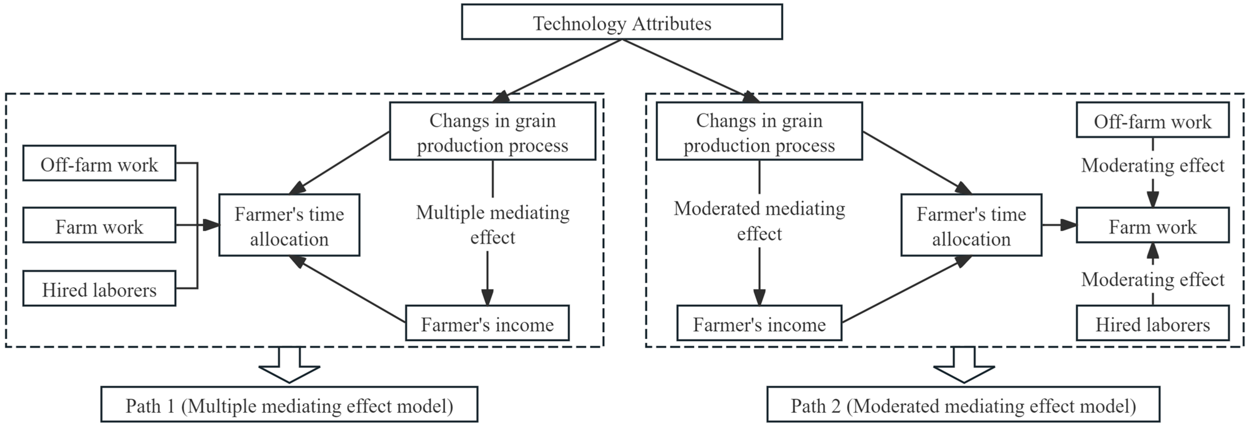
3.1.2. Multiple Mediation Effect Model

In this study, multiple parallel mediating variables between CA technology adoption and farmers are assumed in path 1, and the corresponding model becomes a parallel (multiple) mediation model. According to the theoretical framework, the multiple mediation effect model based on structural equation modeling is used to test the mediating effect of farm households’ time reconfiguration on income, that is, to calculate the indirect effect of the adoption status of different technological attributes (${\mathrm{D}}_{\mathrm{i}}$) on farm households’ income (${\mathrm{Y}}_{\mathrm{i}}$) through three mediating variables, namely the yield effect (${\mathrm{M}}_{1\mathrm{i}}$), transfer effect (${\mathrm{M}}_{2\mathrm{i}}$), and hired labor effect (${\mathrm{M}}_{3\mathrm{i}}$). The average mediating effect (ACME) [64] of the different mediating variables is as follows:

$$ACME\left(D_i\right)=E\left[Y_i\right\{D_i,M_i\left(1\right)\}-Y_i\{D_i,M_i\left(0\right)\left\}\right]$$

(12)

Based on the mechanism of the mediating effect action shown in path 1, the following parallel mediating effect model is developed:

$$M_{1i}=a_1{D}_i+c_{1i}{Z}_i+e_{1i}$$

(13)

$$M_{2i}=a_2{D}_i+c_{2i}{Z}_i+e_{2i}$$

(14)

$$M_{3i}=a_3 D_i+c_{3i}{Z}_i+e_{3}i$$

(15)

$$Y_i=b_1{M}_1+b_2{M}_2+b_3{M}_3+d D_i+c_{4i}{Z}_i+e_{4i}$$

(16)

In equation, ${\mathrm{Z}}_{\mathrm{i}}$ is a set of control variables. In the model, ${\mathrm{a}}_1\times {\mathrm{b}}_1$, ${\mathrm{a}}_2\times {\mathrm{b}}_2,{\mathrm{a}}_3\times {\mathrm{b}}_3,{\mathrm{a}}_1\times {\mathrm{b}}_1+{\mathrm{a}}_2\times {\mathrm{b}}_2+{\mathrm{a}}_3\times {\mathrm{b}}_3$ and $\mathrm{d}$ stand for the output effect, transfer effect, hiring effects, and the direct effect, respectively. The steps of the test are borrowed from the structural equation method proposed by Bartus (2017) for calculating the corresponding values, and the Bootstrap method is later used to test the robustness of the indirect effects [65].

3.1.3. Moderated Mediation Model

In this study, the existence of a regulated mediation mechanism between CA technology adoption and farm households is assumed in path 2. Based on theoretical assumptions, and following the methods of Muller et al. (2005) [66] and Preacher and Hayes (2008) [67], the following equations can be constructed to test for the regulated mediation model, that is, to calculate the indirect effects of the adoption state of different technological attributes (${\mathrm{D}}_{\mathrm{i}}$) mediated by the income of the farm household (${\mathrm{Y}}_{\mathrm{i}}$) through the yield effect (${\mathrm{M}}_{1\mathrm{i}}$), but the cultivation of the farm household’s food crops is regulated in turn by the balance of its temporal allocations among hired laborers (${\mathrm{M}}_{3\mathrm{i}}$) and non-farm laborers (${\mathrm{M}}_{2\mathrm{i}}$):

$$Y_i={\alpha }_0+{\alpha }_1{D}_i+c_{1i}{Z}_i+e_{1i}$$

(17)

$$M_{1i}={\beta }_0+{\beta }_1{D}_i+c_{2i}{Z}_i+e_{2i}$$

(18)

$$Y_i={\theta }_0+{\theta }_1{D}_i+{\theta }_2{M}_{1i}+c_{3i}{Z}_i+e_{3i}$$

(19)

$$Y_i={\gamma }_0+{\gamma }_1{D}_i+{\gamma }_2{M}_{1i}+{\gamma }_3{M}_{2i}+{\gamma }_4{M}_{3i}+{\gamma }_5{M_{1i}M}_{2i}+{\gamma }_6{M_{1i}M}_{3i}+c_{4i}{Z}_i+{\tau }_{ij}$$

(20)

In Equations (17)–(20), the symbols of the corresponding variables are the same as in the above formulas. In Equation (17), the coefficient ${\mathsf{\alpha }}_1$ indicates the total effect of farmers’ technology adoption status on income. In Equation (18), the coefficient ${\mathsf{\beta }}_1$ indicates the yield effect on farmers’ income. In Equations (10) and (20), the coefficients θ1 and γ1 indicate the direct effect of the technology adoption status on the impact of income. By substituting Equation (18) into Equation (19) we can obtain ${\mathsf{\beta }}_1\times {\mathsf{\theta }}_2$, which indicates the indirect effect of the technology adoption status on the income impact (i.e., through the yield effect on the income impact). In Equation (20), the coefficient ${\mathsf{\gamma }}_3$,${\mathsf{\gamma }}_4$ indicates the direct effect of the adjustment variables on the income impact, ${\mathsf{\gamma }}_2+{\mathsf{\gamma }}_5$, ${{\mathsf{\gamma }}_2+\mathsf{\gamma }}_6$ (i.e., mediating efficiency impact on income through the transfer and hiring effects of the adjustment of the yield effect).

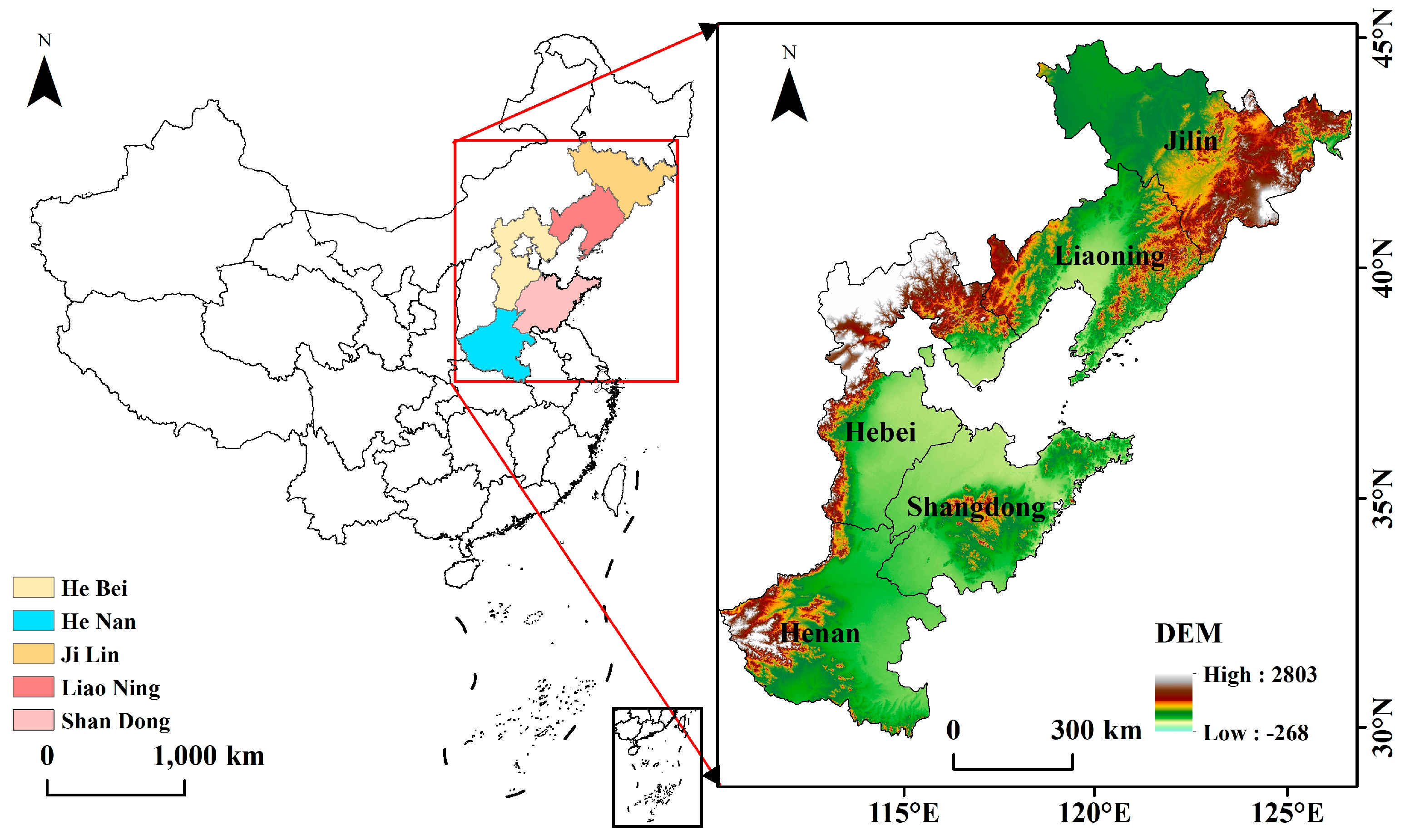
3.2. Data Sources and Descriptive Statistics

This study employed microdata for empirical analysis, sourced from a survey on the adoption of conservation tillage technology among grain farmers. Conducted by China Agricultural University between June and August 2023, the survey encompassed five Chinese provinces: Shandong, Hebei, Henan, Liaoning, and Jilin. To ensure that all subgroups of the sample were proportionally included in the total sample, we reduced the standard error of the overall estimate, and to avoid estimation bias, the study employed stratified random sampling to collect microdata. The questionnaire covered a total of 113 questions in five aspects, including the characteristics of farmers’ families, the cost–benefit of grain production, technology awareness and adoption characteristics, and the development of the villages where the farmers are located. Except for the part on technology awareness and adoption characteristics, which used closed-ended questions, the rest of the questions were open-ended questions.

Utilizing stratified random sampling, the survey initially targeted 1112 participants. Sample households were selected based on the following procedure: In each province, two municipalities with the highest grain production were selected, followed by the random selection of two townships per municipality, two villages per township, and 15–30 grain farmers per village. Individual interviews were conducted with farmers cultivating maize, wheat, and rice. After cleaning the data based on the explanatory variables, explained variables, and control variables, the actual sample size used was 922. The specific study area is shown in Figure 2.

The explanatory variable is the natural logarithm of total household income; it is the link change after technology adoption. The mediating (moderating) variables are the natural logarithm of grain output, non-agricultural income, and labor cost, which are used to measure the yield, transfer, and labor effects, respectively. Referring to the existing studies, the model controls for three types of characteristic variables: personal, household, and business characteristics [68]. Differences in the mean values of the variables are compared between the groups adopting a single type or composite type of technology. To ensure that the endogenous transformation model is identified, the equation for technology adoption uses “number of times receiving technology training” as an instrumental variable, which is consistent with the principle that it is related to CA technology adoption and not farmers’ income. Significant differences are observed among total household income, total food production value, hired labor cost, age of farmers, years of education, gender, number of village cadres and party members in the household, planting scale, fertilizer and pesticide inputs, and number of times farmers received training between single-type and composite technology groups, implying a selective bias.

Table 1. Descriptive statistics of variables.

Variables	Mono-Type Technology Group (D = 0)		Composite Technology Group (D = 1)
	Mean	Standard Deviation	Mean	Standard Deviation
Variable Explained
Natural Logarithm of Total Household Income (y)/RMB	10.48	1.331	10.927 ***	1.398
Mediating (Moderating) Variables
Natural Logarithm of Gross Food Production (M1)/RMB	9.889	1.263	10.277 ***	1.527
Natural Logarithm of Household Non-farm Business Income (M2)/RMB	10.4	1.087	10.316	1.068
Natural Logarithm of the Cost of Domestic Workers (M3)/RMB	7.918	2.161	9.854 ***	2.322
Individual Characteristics
Age/year	59.289	10.078	57.662 *	10.898
Educational Period (Edu)/year	7.547	3.232	8.298 ***	3.103
Gender/(Male = 1; Female = 0)	0.926	0.261	0.889 *	0.314
Technology Preferences (pre)/(Prefer = 1; Neutral = 2; sheltered = 3)	2.272	0.822	2.253	0.824
Planting Period (Year)/year	33.9	14.324	33.599	14.73
Household Characteristics
Total Household Labor Force (Labor)/persons	2.489	1.051	2.44	0.888
Village Cadres in Household (Cadres)/persons	0.111	0.314	0.179 **	0.384
Party Members in Household (Members)/persons	0.182	0.43	0.327 ***	0.573
Operational Characteristics
Farming Days (Day)/day	75.865	52.424	75.563	64.919
Natural Logarithm of Subsidized Amount (Insubsidy)/RMB	7.123	1.374	7.078	1.692
Planting Scale (Land)/Mu	66.434	241.717	144.584 ***	442.357
Natural Logarithm of Total Annual Fertilizer Inputs (lnfer)/RMB	8.18	1.347	8.517 ***	1.649
Natural Logarithm of Total Annual Pesticide Inputs (lnpes)/RMB	6.601	1.536	6.865 *	1.664
Number of Trainings Received (Training times)/class	0.865	2.481	1.581 **	4.153
Observed Value	570		352

Note: *, **, and *** indicate that the t-test is significant at the 10%, 5%, and 1% levels, respectively; the original hypothesis of the t-test is that there are no significant differences between the variables in the single-technology and composite technology groups.

provides definitions and descriptive statistics for the variables.

4. Empirical Results

Table 2. Estimates of the endogenous switching model of technology adoption and income for the full sample of farmers.

Variables	Resulting Equations		Behavioral Equation
	Unitary Technology Group	Composite Technology Group
Age	−0.018 **	−0.009	−0.010
	(0.009)	(0.006)	(0.007)
Edu	−0.036	0.024	0.046 **
	(0.022)	(0.017)	(0.018)
Gender	0.148	0.115	−0.460 ***
	(0.195)	(0.184)	(0.177)
Pre	0.003	−0.131 **	0.027
	(0.074)	(0.058)	(0.064)
Year	−0.009	−0.005	0.012 **
	(0.007)	(0.004)	(0.005)
Labor	0.416 ***	0.473 ***	−0.116 **
	(0.072)	(0.048)	(0.055)
Cadres	0.358 **	0.039	−0.059
	(0.176)	(0.170)	(0.169)
Members	−0.013	0.196	0.226 *
	(0.126)	(0.131)	(0.120)
Day	0.000	−0.002 ***	−0.001
	(0.001)	(0.001)	(0.001)
Subsidy	0.046	0.067	−0.071
	(0.052)	(0.055)	(0.052)
Land	0.000	0.001 **	0.000
	(0.000)	(0.000)	(0.000)
Lnfer	0.089	0.310 ***	0.309 ***
	(0.102)	(0.087)	(0.084)
Lnpes	0.220 ***	0.036	−0.126 *
	(0.074)	(0.063)	(0.065)
Training times	/	/	0.038 **
			(0.017)
Control cropping system	Yes	Yes	Yes
Control hamlet	Yes	Yes	Yes
Constants term	10.373 ***	7.542 ***	−1.985 ***
	(0.968)	(0.626)	(0.688)
ρμ0 (or ρμ1)	−0.645 **	−0.089
LR test	7.08 **

Note: Standard errors of the estimates are in parentheses; *, **, and *** indicate significance at the 10%, 5%, and 1% levels, respectively.

shows the ESR results for the CA technology adoption decision and income impact effect equations. From the model applicability test, the results of ρμ1 and the LR test represent statistical significance at the levels of 5%, indicating an inter-correlation between the behavioral decision and impact effect equations. Thus, the ESR model should be applied to correct for the sample selection bias caused by unobserved factors. The behavioral equation for adoption decision shows that the probability of adopting composite technology is higher for farmers with more years of education, planting experience, party members in the family, and fertilizer input costs, likely because the higher the education level and richer the planting operation, the lower farmers’ resistance to adopting more CA technology. In addition, the need to reduce fertilizer inputs and opportunities to receive education on cropland protection policies will promote the adoption of more CA technologies among farmers.

The estimation results for single-type and composite technology groups indicate that farmers’ age, number of household laborers and village cadres, pesticide inputs, risk preference, farming season length, cultivation scale, and fertilizer inputs are the key determinants of farmers’ income. To summarize these findings, first, farmers’ farming preferences and experiences are key to their technology adoption. Generally, farmers with a higher degree of accumulated specialized technology experience and greater willingness to try new technologies have higher incomes. Second, crop cultivation scale and fertilizer and pesticide inputs have clear income-generating effects. Third, the more party members and village cadres in the household, the stronger the income-generating effect of technology use and the higher the likelihood of composite CA technology use, owing to the higher likelihood of exposure to new policies and technologies, which is a crucial factor in generating income.

Several aspects of CA technology rely on mechanical equipment, and adopting composite CA technology means that different mechanical facilities or hired labor are needed to complete it [69] (Liu et al., 2021), which increases the operating costs. Moreover, land size and location and number of parcels limit large-scale farmers’ adoption of CA technology [70] (Jiang et al., 2018), requiring further examination to determine whether operation scale differs among farmers adopting different technology attributes. Given that the sown area of crops in the study sample did not show a standard normal distribution, the differences in the planted area between groups adopting different technological attributes were examined based on one-way ANOVA after logit. The results in

Table 3. Supplementary notes on sample distribution and differences in planting size.

Sample Group	Sample Size	Sample Mean	Standard Deviation	ANOVA
Unitary Technology Group	570	66.43419	241.7165	F-Value (Logarization)	p-Value (Logarization)
Composite Technology Group	352	144.5841	442.3572	10.13	0.0015

show a difference in the planted area between farmers adopting the single type of technology and those adopting the composite type. Thus, we performed a descriptive analysis of the sown area of the two types of adoption, finding that large-scale farmers are more likely to adopt composite-type technology, whereas small-scale farmers are more likely to adopt single-type technology.

Based on the counterfactual analytical framework, the estimated average treatment effects for the monotype and composite technology groups are shown in

Table 4. Estimates of treatment effects on farm household income by CA technique adoption for the full sample.

Sample Group	Decision-Making Phase		ATT	ATU
	Ring Changed	Ring Unchanged
Composite Technology Group	10.934 (0.061)	10.366 (0.068)	0.567 ***
Unitary Technology Group	11.824 (0.042)	10.415 (0.046)		1.408 ***

Note: Treatment effect estimates in the table are natural logarithms; Standard errors of the estimates are in parentheses; *, **, and *** indicate significance at the 10%, 5%, and 1% levels, respectively.

. To characterize the income effects of different types of technology attributes more concretely, Figure A1 presents the probability density distributions of incomes in the two groups for both the factual and counterfactual scenarios. In logarithmic form, the average treatment effect (ATT) of income for the composite technology group is 0.567, while that for the non-adoption group (ATU) is 1.408. Details of the revenue density distribution of the different technology type subgroups are represented in Figure A1 in Appendix A. Combining the results of the income effects with the characteristics of the sample distribution based on operation size suggests that if small-scale farmers have already adopted a single-type technology, the overlapping adoption of a composite technology will lead to more pronounced income growth. However, if farmers shift from monotype to composite technology, the income increase effect is not significant. Increased operating costs and an expectation of insignificant scale effects may initially explain why most farmers are reluctant to adopt more CA technologies or even abandon them after initial adoption.

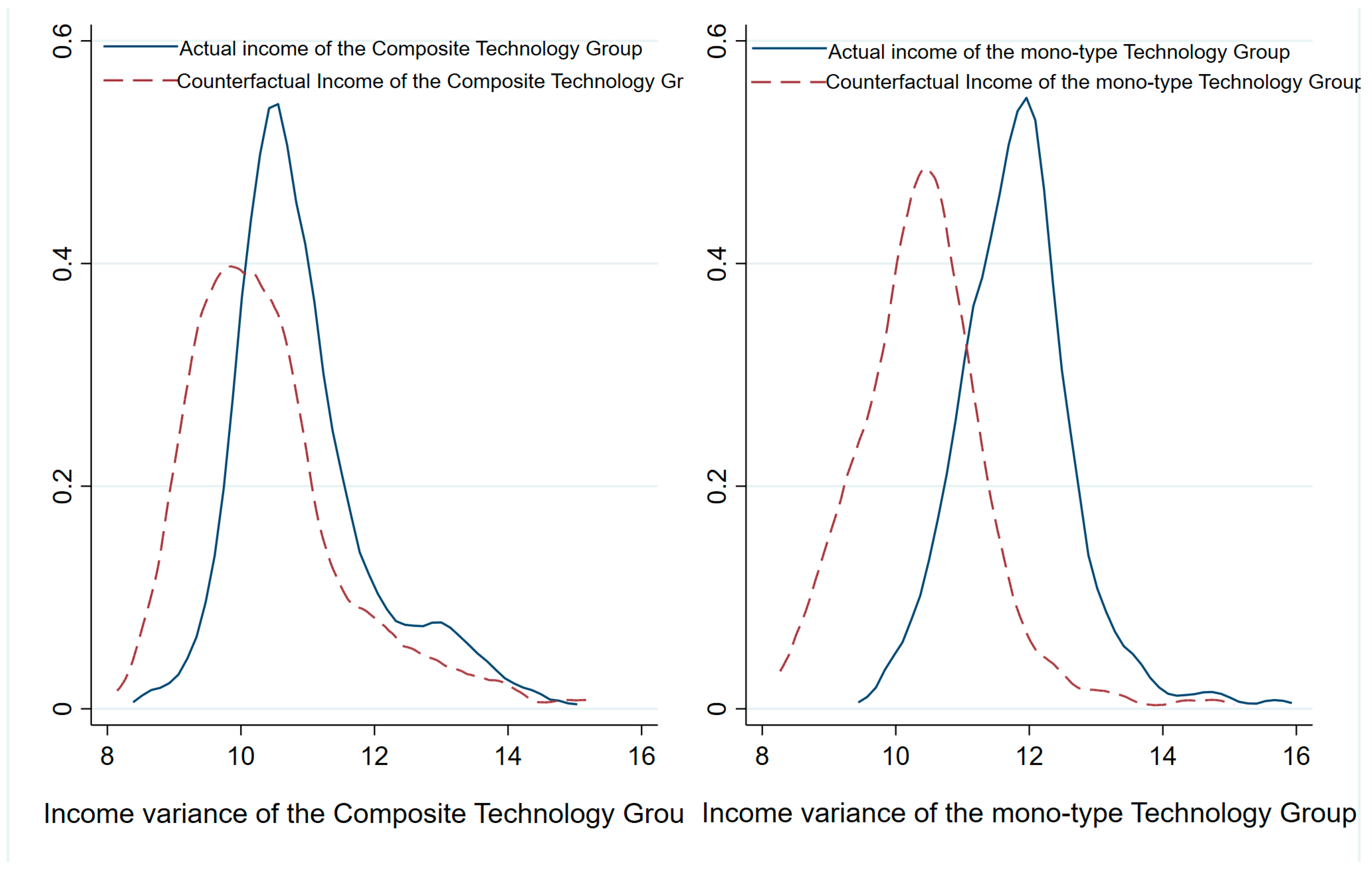
4.1. Heterogeneity Analysis of Income Effects Based on Different Crop Cultivation Types

Different crops have different growth cycles and production characteristics; therefore, we performed a heterogeneity analysis with maize and wheat (the amount of rice planted in the sample area was small and not representative) to verify whether the above conclusions show the same income effect characteristics among farmers growing different crops. The results in

Table 5. Heterogeneity analysis of income effects based on different crop cultivation types.

Sample Group		Decision-Making Phase		Process Effect
		Ring Changed	Ring Unchanged
Maize	Composite Technology Group	10.947 (0.062)	12.108 (0.064)	−1.160 ***
	Unitary Technology Group	11.021 (0.049)	10.048 (0.048)	0.478 ***
Wheat	Composite Technology Group	10.673 (0.063)	12.992 (0.065)	−2.319 ***
	Unitary Technology Group	10.677 (0.063)	10.192 (0.067)	0.485 ***

Note: Standard errors of the estimates are in parentheses; *, **, and *** indicate significance at the 10%, 5%, and 1% levels, respectively.

show that, regardless of whether wheat or maize is grown, farmers adopting composite technologies do not experience better income effects than those adopting mono technologies, leading to a decrease in income. The results robustly support the above conclusion that adopting composite technologies does not result in better income effects than adopting mono technologies, implying that CA technologies that rely on specialized agricultural machinery do not have the same benefits of scale that other green production technologies in agriculture have when used in a stacked manner.

4.2. Parallel Mediation of Multiple Effects and Robustness Tests

Based on the significant income-generating effect of technology adoption on farm household income, this study analyzed whether a mediating mechanism exists in which differences in CA technology segments affect farm household income through household time allocation, that is, whether there is a multi-effect parallel mediating mechanism of the yield effect (M₁), transfer (M₂), and hired labor (M₃) effects. Referring to the multiple mediation effect test model established by Macho and Lederman (2011) based on structural equations, the indirect effects on farm household income were analyzed [71]. The total effect not shown in

Table 6. Multiple effects—mediation effect tests for parallel (multiple) mediators.

Variables	X	M1	M2	M3
Adj	0.252	0.196 ***	−0.065	0.282
	(0.245)	(0.019)	(0.105)	(0.941)
M1	0.339 ***
	(0.077)
M2	0.390 ***
	(0.062)
M3	−0.022
	(0.108)
Control variable	Yes	Yes	Yes	Yes
Control cropping systems	Yes	Yes	Yes	Yes
Control village-level features	Yes	Yes	Yes	Yes
Constant term	0.835	3.873 ***	9.629 ***	−0.523
	(0.762)	(0.391)	(0.439)	(0.275)
Estimated error variance	0.245 ***	0.527 ***	0.899 ***	1.925 ***
	(0.012)	(0.011)	(0.052)	(0.071)

Note: Standard errors of the estimates are in parentheses; *, **, and *** indicate significance at the 10%, 5%, and 1% levels, respectively.

is that of the impact of technology adoption on farm household income, as shown in the third column of behavioral equations in Table 2.

The parallel mediation results suggest that only the yield effect is a partial mediator if the parallel mediation effect model is used. The direct effect of the technology attributes on income in column (1) of Table 6 is 0.252, but not significant (i.e., a masking effect). The direct yield effect on farmers’ income is 0.339 and significant at the 1% level, and multiplying it with the estimated coefficient of M₁ in column (2) of Table 6 shows a mediating yield effect on farmers’ income of 0.066, which is 14.9% of the mediating effect. This indicates that adopting different technology attributes raises income by approximately 15% by increasing the yield effect. However, the subsequent results of the bootstrap test shown in

Table A1. Results of self-help method test for parallel (multiple) mediation.

Self-Help Method Test		Constant	Bias	Standard Error	95% Confidence Interval	Bias-Corrected Confidence Interval
Indirect effect	M1	−0.006	0.002	0.083	[−0.186, 0.149]	[−0.320, 0.107]
	M2	0.066	0.003	0.062	[−0.034, 0.266]	[−0.013, 0.254]
	M3	−0.025	−0.001	0.048	[−0.134, 0.052]	[−0.175, 0.041]
Direct effect		0.252	−0.073	0.450	[−0.744, 1.181]	[−0.456, 0.149]

in Appendix A indicate that none of the indirect effects of the three mediating variables were found to be significant, and that the results are not robust. Overall, the mediation mechanism of the yield effect, hiring effect, and three effects in parallel, as hypothesized in path 1, is not advisable. However, because the yield effect has a mediating role, the study continues to try to restart the parallel mediation effect test by reducing the number of effects.

The mediation effect test results in

Table 7. Parallel mediation effect tests for yield efficiency, transfer effects.

Variables	X		M1	M2
Adj	0.275		0.196 ***	−0.065
	(0.149)		(0.019)	(0.105)
M1	0.312 ***
	(0.032)
M2	0.513 ***
	(0.024)
Control variable	Yes		Yes	Yes
Control cropping systems	Yes		Yes	Yes
Control village-level features	Yes		Yes	Yes
Constant term	2.296 ***		3.873 ***	9.629 ***
	(0.168)		(0.391)	(0.439)
Estimated error variance	0.314 ***		0.527 ***	0.899 ***
	(0.090)	(0.011)	(0.052)

Note: Standard errors of the estimates are in parentheses; *, **, and *** indicate significance at the 10%, 5%, and 1% levels, respectively.

and

Table 8. Parallel mediation effect tests for yield benefits, hiring effects.

Variables	X	M1	M3
Adj	0.061	0.196 ***	0.282
	(0.087)	(0.019)	(0.941)
M1	0.405 ***
	(0.048)
M3	−0.064
	(0.131)
Control variables	Yes	Yes	Yes
Control cropping systems	Yes	Yes	Yes
Control village-level features	Yes	Yes	Yes
Constant term	4.132 ***	3.873 ***	−0.523
	(0.420)	(0.391)	(0.275)
Estimated error variance	0.492 ***	0.527 ***	1.925 ***
	(0.095)	(0.011)	(0.071)

Note: Standard errors of the estimates are in parentheses; *, **, and *** indicate significance at the 10%, 5%, and 1% levels, respectively.

suggest similar conclusions for the parallel mediation effect test results of the yield and transfer effects, as well as yield and hired labor effects. The yield effect is still significant mediation; the mediation effect value and the overall change in the value of the effect ratio are insignificant, and the rest of the effects still do not play a mediating role. After conducting bootstrap tests on the above two parallel mediation models (the results reported, respectively, in

Table A2. Results of the self-help method test for parallel mediation of yield benefits and transfer effects.

		Constant	Bias	Standard Error	95% Confidence Interval	Bias-Corrected Confidence Interval
Indirect effect	M2	−0.033	0.023	0.040	[−0.080, 0.097]	[−0.080, 0.004]
Indirect effect	M1	0.061 ***	0.023	0.021	[0.035, 0.106]	[0.035, 0.106]
Direct effect		0.302	0.023	0.067	[0.190, 0.453]	[0.190, 0.401]

Note: Standard errors of the estimates are in parentheses; *, **, and *** indicate significance at the 10%, 5%, and 1% levels, respectively.

and

Table A3. Results of self-help method test for parallel mediation of yield benefits and hiring effects.

		Constant	Bias	Standard Error	95% Confidence Interval	Bias-Corrected Confidence Interval
Indirect effect	M3	−0.061	0.070	0.030	[−0.054, 0.060]	[−0.054, 0.009]
Indirect effect	M1	0.080 ***	0.004	0.044	[0.017, 0.181]	[0.028, 0.133]
Direct effect		0.122	0.093	0.264	[−0.115, 0.918]	[−0.115, 0.918]

Note: Standard errors of the estimates are in parentheses; *, **, and *** indicate significance at the 10%, 5%, and 1% levels, respectively.

in Appendix A), the transfer and hiring effects of the indirect effect remain insignificant, indicating that even if the number of parallel effects is reduced, it still fails the test. This means that the theoretical assumption that CA technology with different attributes acts on farm household income through multiple intermediaries affecting the allocation of hired labor time and family time is not reasonable (i.e., path 1 is invalid).

After two separate parallel mediation tests found potential problems with path 1, to clarify whether different types of time allocation, respectively, mediate the path of farmers’ income, the mediation effect of the three effects of the regression was tested. After the stepwise regression test, the results of the yield effect remain robust to play a part in the mediating role. The mediating effect is 10.6%. Column (3) in

Table 9. Mediating effects test of yield, transfer, and hired labor effects.

		Yield Effect		Transfer Effect		Hired Labor Effect
	x	M1	X	M2	x	M3	x
Adj	0.441 ***	0.235 ***	0.328 ***	−0.077	0.454 ***	0.309	0.082
	(0.079)	(0.061)	(0.075)	(0.105)	(0.064)	(0.456)	(0.259)
M1			0.453 ***
			(0.046)
M2					0.528 ***
					(0.030)
M3							−0.075
							(0.064)
Control variables	Yes	Yes	Yes	Yes	Yes	Yes	Yes
Control cropping systems	Yes	Yes	Yes	Yes	Yes	Yes	Yes
Control village-level features	Yes	Yes	Yes	Yes	Yes	Yes	Yes
Constant term	7.010 ***	3.932 ***	5.254 ***	9.600 ***	3.611 ***	−0.528	6.285 ***
	(0.445)	(0.343)	(0.458)	(0.551)	(0.445)	(2.089)	(1.173)
Adj R-squared	0.526	0.706	0.586	0.212	0.682	0.624	0.771

Note: Standard errors of the estimates are in parentheses; *, **, and *** indicate significance at the 10%, 5%, and 1% levels, respectively.

shows that after adopting composite CA technology, crop production increased by 0.453%, increasing household income by 0.328%. The transfer effect plays a masking effect; the masking effect of the ratio of 19.9% in Column (5) of Table 9 demonstrates that differences in the number of hours worked in the non-farm sector significantly widen the income differentials between the respective groups after farmers adopt CA technologies with different attributes. The hired labor effect is stable and plays no role. Similarly, after carrying out the bootstrap method test on the three groups of mediating effects in separate steps, the results displayed in

Table A4. Bootstrap method test results for separate intermediaries.

Self-Help Method Test		Constant	Bias	Standard Error	95% Confidence Interval	Bias-Corrected Confidence Interval
Indirect effect	M1	−0.249 ***	0.003	0.171	[−0.611, 0.067]	[−0.660, 0.041]
	M2	−0.071 ***	−0.005	0.135	[−0.407, 0.121]	[−0.504, 0.073]
	M3	0.278	−0.051	0.701	[−1.117, 1.963]	[−0.439, 2.443]
Direct effect	M1	3.126	0.291	1.033	[1.182, 5.208]	[1.092, 5.136]
	M2	4.454	−0.020	1.373	[1.900, 7.121]	[1.900, 7.121]
	M3	1.926	−0.029	3.271	[−5.071, 8.204]	[−5.515, 7.923]

Note: Standard errors of the estimates are in parentheses; *, **, and *** indicate significance at the 10%, 5%, and 1% levels, respectively.

in Appendix A show significant indirect yield and transfer effects, whereas the indirect hired labor effect remains non-significant. The total effect of technology attributes on farmers’ income is significant; therefore, the reallocation of family time (i.e., yield and transfer effects) can further explain the relationship between technology attributes and farmers’ household income. Based on the assumption of path 2, farmers’ allocation of hired labor and household time may affect yields, and combined with the parallel mediation test, this suggests that the yield effect, as the main mediating effect variable, is in the causal chain between technology attributes and farm household income. The transfer and employment effects participate in the mechanism between technology and income [72], and they play a moderating role. Therefore, the moderated mediation effect test will be performed in the next empirical link.

4.3. Moderated Mediation Effect Test

To examine the moderating effect of farmers’ time allocation to hired and household fixed-time labor on the food production affecting farmers’ income, interaction terms based on food production, non-farm income, and hired labor costs were constructed. Equation (20) was estimated using structural equation modeling, the results of which are shown in

Table 10. Moderating transfer and hiring effects.

Variables	Non-Farm Income		Hired Labor Costs
	(1)	(2)	(3)	(4)
	M1	M2	M1	M3
Adj	0.238 ***	1.020 ***	−0.034	0.528 **
	(0.076)	(0.210)	(0.189)	(0.259)
M1		0.357 ***		0.096
		(0.059)		(0.218)
M2	1.191 ***
	(0.193)
M1×M2		−0.070 ***
		(0.020)
M3			0.067
			(0.317)
M1×M3				−0.012
				(0.027)
Control variables	Yes	Yes	Yes	Yes
Controll cropping systems	Yes	Yes	Yes	Yes
Controll village-level features	Yes	Yes	Yes	Yes
Constant term	4.336 ***	4.895 ***	−3.861 *	3.579
	(0.457)	(0.913)	(2.092)	(2.474)
Log likelihood	−18,294.87		−43,754.63
Estimated error variance	0.492 ***	0.283 ***	0.363 ***	0.482 ***
	(0.033)	(0.019)	(0.054)	(0.071)

Note: Standard errors of the estimates are in parentheses; *, **, and *** indicate significance at the 10%, 5%, and 1% levels, respectively.

. The coefficient of the interaction term in column (2) of Table 10 is negative and significant at the 1% level, indicating that the non-farm time allocation of farmers negatively moderates the positive effect of food production on farm business income. Every 1% increase in non-farm income will reduce the positive yield effect on farm income by 0.07%. Furthermore, the interaction term regression coefficient in column (4) of Table 10 is not significant, implying that the labor allocation of hired time to grain yield affects farm household income; this path does not exist. The possible reason is that CA has already realized the entire process of cultivation machinery operation in China, and hiring implies that the machinery and equipment are rented at the same time for the operation. Under the guarantee of comprehensive land subsidies in the agricultural sector and subsidies of agricultural machinery for the adoption of CA technology, the potential impact on food production (yield effect) has been able to cancel out the hiring effect.

Non-farm income and hiring costs are both continuous variables; therefore, the moderating yield effect at different levels of non-farm income and hiring costs are tested after decentering the data. The results reported in

Table A5. Changes in the moderating effect of non-farm income at different levels.

	Constant	Bias	Standard Error	95% Confidence Interval	Bias-Corrected Confidence Interval
Mean − 1SD	0.088 ***	−0.002	0.033	[0.028, 0.154]	[0.034, 0.166]
Mean	0.069 ***	−0.002	0.026	[0.023, 0.120]	[0.028, 0.133]
Mean + 1SD	0.051 **	−0.001	0.021	[0.013, 0.094]	[0.018, 0.103]

Note: Standard errors of the estimates are in parentheses; *, **, and *** indicate significance at the 10%, 5%, and 1% levels, respectively.

and

Table A6. Regulatory changes in hiring costs at different levels.

	Constant	Bias	Standard Error	95% Confidence Interval	Bias-Corrected Confidence Interval
Mean − 1SD	−0.014	−0.009	0.109	[−0.025, 0.177]	[−0.291, 0.170]
Mean	−0.014	−0.009	0.108	[−0.260, 0.179]	[−0.278, 0.171]
Mean + 1SD	−0.013	−0.010	0.107	[−0.266, 0.188]	[−0.269, 0.171]

in Appendix A show that the mediating role of the yield effect decreases as the non-farm income reaches a certain threshold; after all, it is not possible for farmers to allocate all their time to participate in non-farm labor without ensuring the sustainability of their farming practices. This is simultaneously echoed by the results of endogenous switching, superimposed on CA technology adoption, which may lead to the excessive crowding out of labor while reducing income levels.

5. Conclusions and Discussion

5.1. Conclusions

The main conclusions are as follows. First, after farmers adopt CA technologies with different attributes, the income-generating effect decreases. This effect is weaker for farmers adopting composite technology than for those adopting single-type technology because the technology is more dependent on complex machinery and equipment. Furthermore, the superposition of adopting CA technology with different attributes does not optimize the production link for farmers, resulting in the income-generating effect being diluted by the complex technology link. Second, regarding mediating effects, composite technology adoption showed no significant effect on the cost of hiring labor and mainly produced yield and transfer effects. Third, in terms of yield effects, adopting composite technology promoted a simultaneous increase in food production and income, which is consistent with the conclusion of a previous study on CA technology [73]. Fourth, regarding transfer effects, after CA technology adoption, prompting non-farm labor negatively moderates the yield effect on farm household income and widens the income differences between adoption groups to some extent. Thus, after households in the sample adopted composite CA technology, time reallocation increased household labor and caused a decrease in non-farm sector work, whereas the hired labor time remained unchanged. In addition, repeated validation of the constructed endogenous switching model and bootstrap tests based on varietal heterogeneity also demonstrated the robustness of the findings.

This study clarifies the impact of technology adoption, hidden behind the characteristics of technological attributes, on farmers’ income, and analyzes the reasons for income differences from the perspective of time allocation, thus expanding the boundaries of the existing research. The research results confirm that the adoption of complex combined technologies has a significant negative impact on income, but the dynamic effect of this impact over time remains unclear. Future research should investigate whether the long-term superposition use of CA technology by farmers affects income through panel data.

5.2. Discussion

The results of this study provide detailed insights into the relationship between the adoption of CA technology and farmers’ income. First, it was observed that the income-generating effect of farmers adopting composite CA technology weakened, which can be attributed to their higher degree of dependence on complex machinery and equipment. This result is consistent with previous studies, indicating that an increase in technological complexity often brings operational challenges and may dilute productivity gains, especially for small-scale farmers [16]. Similarly, Pannell et al. (2014) emphasized that mechanical complexity and technological mismatch are important economic factors hindering the widespread income-increasing effect of conservation agriculture [74]. Gallardo and Sauer (2018) also pointed out that the uncertainty of the return on investment in agricultural machinery reduces the actual economic benefits after technology adoption [75]. Although theoretically the composite technology should achieve production synergies, empirical evidence shows that the superimposed application actually increases operational complexity and dilutes the revenue-generating effect. After farmers adopted multiple CA technologies in a superimposed manner, due to the lack of coordinated management, the labor input increased ineffectively, and the net income growth was not significant [76]. On the other hand, the imperfection of the market and management chains makes it difficult to realize the potential benefits of the composite technology in the small-scale farming system; without full integration in the production process, the superimposed technologies instead increase management complexity and operational errors [77,78].

The research shows that composite technology has a relatively small impact on the time allocation of hired labor. Instead, it mainly functions through promoting output growth (output effect) and changes in household labor allocation (transfer effect). In fact, the income increase in traditional agriculture after the adoption of CA technology mainly stems from output growth rather than changes in hiring costs [79]. Meanwhile, the labor market’s response after technology adoption is complex, but the direct change in the external hiring demand is usually not significant. Simultaneously, the return of household labor to agriculture is also a common phenomenon after technology adoption [80,81]. However, it should be noted that the adoption of composite technologies prompts the transfer of household labor from the non-agricultural sector, thus negatively moderating the positive income effect brought about by yield improvement and widening the income gap among adopters. There are differences in labor reallocation and capital acquisition capabilities among different farmers, and technology promotion actually exacerbates income inequality [82]. During the technology diffusion process, the imperfect labor market leads to further differentiation in the income levels of different farmers [83]. Overall, these results emphasize that although the integrated protection technology offers agronomic benefits, its economic impact depends on the technological complexity, labor dynamics, and market opportunities faced by rural households. Therefore, this study not only supports the findings of previous research, but also provides new evidence on how the labor reallocation mechanism affects the outcomes of technology adoption, offering a new perspective for policy interventions aimed at promoting inclusive rural development.

Some insights can be drawn based on the above discussion. First, to promote CA technology, the government should ensure that farmers can improve efficiency by replacing human labor with machinery after overlapping the use of different technologies, and the technical training for farmers should be strengthened. As a sustainable production technology with a technical threshold, more CA measures may increase farmers’ cultivation difficulties, while weakening the effects of increasing production and income [84]. Second, agricultural socialization services with attached machinery operators should be provided to help large-scale farmers complete the more time-consuming and labor-intensive production aspects of CA technology, allowing farmers to have more energy to reallocate time to non-farming activities [85]. Third, the rural labor force is an increasingly aging population. Against the background of an aging rural labor force and the further slowing down of the transfer effects, it is necessary to further optimize the environment of the food trading and labor markets, so that farmers can feel that it is profitable to grow food and implement CA to make them more flexible in switching between engaging in food production and non-farm employment [86]. Combining these three measures will encourage more farmers to use CA technology while realizing steady increases in production and income.

References

1. Pretty, J.N.; Noble, A.D.; Bossio, D.; Dixon, J.; Hine, R.E.; de Vries, F.; Morison, J.I.L. Resource-Conserving Agriculture Increases Yields in Developing Countries. Environ. Sci. Technol. 2006, 40, 1114–1119. [Google Scholar] [CrossRef] [PubMed]
2. Pittelkow, C.; Linquist, B.; Lundy, M.; Liang, X.; Groenigen, K.J.; Lee, J.; Gestel, N.; Six, J.; Venterea, R.; Kessel, C. When Does No-till Yield More? A Global Meta-Analysis. Field Crop. Res. 2015, 183, 156–168. [Google Scholar] [CrossRef]
3. Lestrelin, G.; Hoa, T.Q.; Jullien, F.; Rattanatray, B.; Khamxaykhay, C.; Tivet, F. Conservation Agriculture in Laos: Diffusion and Determinants for Adoption of Direct Seeding Mulch-Based Cropping Systems in Smallholder Agriculture. Renew. Agric. Food Syst. 2012, 27, 81–92. [Google Scholar] [CrossRef]
4. Kienzler, K.M.; Lamers, J.P.A.; McDonald, A.; Mirzabaev, A.; Ibragimov, N.; Egamberdiev, O.; Ruzibaev, E.; Akramkhanov, A. Conservation Agriculture in Central Asia-What Do We Know and Where Do We Go from Here? Field Crop. Res. 2012, 132, 95–105. [Google Scholar] [CrossRef]
5. Ataei, P.; Sadighi, H.; Chizari, M.; Abbasi, E. Analysis of Farmers’ Social Interactions to Apply Principles of Conservation Agriculture in Iran: Application of Social Network Analysis. J. Agric. Sci. Technol. 2019, 21, 1657–1671. [Google Scholar]
6. Khan, Z.; Midega, C.; Pittchar, J.; Pickett, J.; Bruce, T. Push-Pull Technology: A Conservation Agriculture Approach for Integrated Management of Insect Pests, Weeds and Soil Health in Africa UK Government’s Foresight Food and Farming Futures Project. Int. J. Agric. Sustain. 2011, 9, 162–170. [Google Scholar] [CrossRef]
7. Latifi, S.; Hauser, M.; Raheli, H.; Moghaddam, S.M.; Viira, A.-H.; Ozuyar, P.G.; Azadi, H. Impacts of Organizational Arrangements on Conservation Agriculture: Insights from Interpretive Structural Modeling in Iran. Agroecol. Sustain. Food Syst. 2021, 45, 86–110. [Google Scholar] [CrossRef]
8. Zhang, F.; Bei, J.; Shi, Q.; Wang, Y.; Wu, L. Research on Agricultural Machinery Services for the Purpose of Promoting Conservation Agriculture: An Evolutionary Game Analysis Involving Farmers, Agricultural Machinery Service Organizations and Governments. Agriculture 2024, 14, 1383. [Google Scholar] [CrossRef]
9. Li, H.; He, J.; Bharucha, Z.P.; Lal, R.; Pretty, J. Improving China’s Food and Environmental Security with Conservation Agriculture. Int. J. Agric. Sustain. 2016, 14, 377–391. [Google Scholar] [CrossRef]
10. Jat, S.L.; Parihar, C.M.; Singh, A.K.; Nayak, H.S.; Meena, B.R.; Kumar, B.; Parihar, M.D.; Jat, M.L. Differential Response from Nitrogen Sources with and without Residue Management under Conservation Agriculture on Crop Yields, Water-Use and Economics in Maize-Based Rotations. Field Crops Res. 2019, 236, 96–110. [Google Scholar] [CrossRef]
11. Borbón-Gracia, A.; Lugo-García, G.A.; Reyes-Olivas, Á.; Valenzuela-Herrera, V.; Sauceda-Acosta, C.P. Wheat, Maize and Safflower Rotation in Conservation Tillage vs. Traditional Tillage. Rev. Fitotec. Mex. 2020, 43, 371–378. [Google Scholar] [CrossRef]
12. Ruzzante, S.; Labarta, R.; Bilton, A. Adoption of Agricultural Technology in the Developing World: A Meta-Analysis of the Empirical Literature. World Dev. 2021, 146, 105599. [Google Scholar] [CrossRef]
13. Ramsey, S.M.; Bergtold, J.S.; Canales, E.; Williams, J.R. Effects of Farmers’ Yield-Risk Perceptions on Conservation Practice Adoption in Kansas. J. Agric. Resour. Econ. 2019, 44, 380–403. [Google Scholar]
14. Liben, F.M.; Wortmann, C.S.; Tirfessa, A. Geospatial Modeling of Conservation Tillage and Nitrogen Timing Effects on Yield and Soil Properties. Agric. Syst. 2020, 177, 102720. [Google Scholar] [CrossRef]
15. Zhang, H.; Hobbie, E.A.; Feng, P.; Zhou, Z.; Niu, L.; Duan, W.; Hao, J.; Hu, K. Responses of Soil Organic Carbon and Crop Yields to 33-Year Mineral Fertilizer and Straw Additions under Different Tillage Systems. Soil Tillage Res. 2021, 209, 104943. [Google Scholar] [CrossRef]
16. Tambo, J.A.; Mockshell, J. Differential Impacts of Conservation Agriculture Technology Options on Household Income in Sub-Saharan Africa. Ecol. Econ. 2018, 151, 95–105. [Google Scholar] [CrossRef]
17. Corbeels, M.; Naudin, K.; Whitbread, A.M.; Kühne, R.; Letourmy, P. Limits of Conservation Agriculture to Overcome Low Crop Yields in Sub-Saharan Africa. Nat. Food 2020, 1, 447–454. [Google Scholar] [CrossRef]
18. Corbeels, M.; de Graaff, J.; Ndah, T.H.; Penot, E.; Baudron, F.; Naudin, K.; Andrieu, N.; Chirat, G.; Schuler, J.; Nyagumbo, I.; et al. Understanding the Impact and Adoption of Conservation Agriculture in Africa: A Multi-Scale Analysis. Agric. Ecosyst. Environ. 2014, 187, 155–170. [Google Scholar] [CrossRef]
19. Ngoma, H.; Angelsen, A.; Jayne, T.S.; Chapoto, A. Understanding Adoption and Impacts of Conservation Agriculture in Eastern and Southern Africa: A Review. Front. Agron. 2021, 3, 671690. [Google Scholar] [CrossRef]
20. Lalani, B.; Dorward, P.; Holloway, G. Farm-Level Economic Analysis—Is Conservation Agriculture Helping the Poor? Ecol. Econ. 2017, 141, 144–153. [Google Scholar] [CrossRef]
21. Huang, K.; Cao, S.; Qing, C.; Xu, D.; Liu, S. Does Labour Migration Necessarily Promote Farmers’ Land Transfer-in?—Empirical Evidence from China’s Rural Panel Data. J. Rural. Stud. 2023, 97, 534–549. [Google Scholar] [CrossRef]
22. Becker, G.S. A Theory of the Allocation of Time. Econ. J. 1965, 75, 493–517. [Google Scholar] [CrossRef]
23. Mincer, J. Labor Force Participation of Married Women: A Study of Labor Supply. In Aspects of Labor Economics; Princeton University Press: Princeton, NJ, USA, 1962; pp. 63–105. [Google Scholar]
24. Singh, I.; Squire, L.; Strauss, J. A Survey of Agricultural Household Models: Recent Findings and Policy Implications. World Bank Econ. Rev. 1986, 1, 149–179. [Google Scholar] [CrossRef]
25. Fontes, F.P. Soil and Water Conservation Technology Adoption and Labour Allocation: Evidence from Ethiopia. World Dev. 2020, 127, 104754. [Google Scholar] [CrossRef]
26. Zhang, L.; Song, J.; Hua, X.; Li, X.; Ma, D.; Ding, M. Smallholder Rice Farming Practices across Livelihood Strategies: A Case Study of the Poyang Lake Plain, China. J. Rural. Stud. 2022, 89, 199–207. [Google Scholar] [CrossRef]
27. Addison, M.; Ohene-Yankyera, K.; Aidoo, R. Quantifying the Impact of Agricultural Technology Usage on Intra-Household Time Allocation: Empirical Evidence from Rice Farmers in Ghana. Technol. Soc. 2020, 63, 101434. [Google Scholar] [CrossRef]
28. Su, W.; Eriksson, T.; Zhang, L.; Bai, Y. Off-Farm Employment and Time Allocation in on-Farm Work in Rural China from Gender Perspective. China Econ. Rev. 2016, 41, 34–45. [Google Scholar] [CrossRef]
29. Rosales-Salas, J.; Jara-Díaz, S.R. A Time Allocation Model Considering External Providers. Transp. Res. Part B Methodol. 2017, 100, 175–195. [Google Scholar] [CrossRef]
30. Cochrane, W.W. Farm Prices: Myth and Reality; University of Minnesota Press: Minneapolis, MN, USA, 1958. [Google Scholar]
31. Hayami, Y.; Herdt, R.W. Market Price Effects of Technological Change on Income Distribution in Semisubsistence Agriculture. Am. J. Agric. Econ. 1977, 59, 245–256. [Google Scholar] [CrossRef]
32. Schultz, T.W. Transforming Traditional Agriculture: Reply. Am. J. Agric. Econ. 1966, 48, 1015–1018. [Google Scholar] [CrossRef]
33. Ngoma, H. Does Minimum Tillage Improve the Livelihood Outcomes of Smallholder Farmers in Zambia? Food Secur. 2018, 10, 381–396. [Google Scholar] [CrossRef]
34. Miah, M.A.M.; Bell, R.W.; Haque, E.; Rahman, M.W.; Sarkar, M.A.R.; Rashid, M.A. Conservation Agriculture Practices Improve Crop Productivity and Farm Profitability When Adopted by Bangladeshi Smallholders in the Eastern Gangetic Plain. Outlook Agric. 2023, 52, 11–21. [Google Scholar] [CrossRef]
35. Wawire, A.W.; Csorba, Á.; Tóth, J.A.; Michéli, E.; Szalai, M.; Mutuma, E.; Kovács, E. Soil Fertility Management among Smallholder Farmers in Mount Kenya East Region. Heliyon 2021, 7, e06488. [Google Scholar] [CrossRef] [PubMed]
36. Bhatt, R.; Singh, P.; Hossain, A.; Timsina, J. Rice–Wheat System in the Northwest Indo-Gangetic Plains of South Asia: Issues and Technological Interventions for Increasing Productivity and Sustainability. Paddy Water Environ. 2021, 19, 345–365. [Google Scholar] [CrossRef]
37. Sun, L.; Wang, S.; Zhang, Y.; Li, J.; Wang, X.; Wang, R.; Lyu, W.; Chen, N.; Wang, Q. Conservation Agriculture Based on Crop Rotation and Tillage in the Semi-Arid Loess Plateau, China: Effects on Crop Yield and Soil Water Use. Agric. Ecosyst. Environ. 2018, 251, 67–77. [Google Scholar] [CrossRef]
38. Si, R.; Yao, Y.; Zhang, X.; Lu, Q.; Aziz, N. Exploring the Role of Contiguous Farmland Cultivation and Adoption of No-Tillage Technology in Improving Transferees’ Income Structure: Evidence from China. Land 2022, 11, 570. [Google Scholar] [CrossRef]
39. Somasundaram, J.; Sinha, N.; Dalal, R.; Lal, R.; Mohanty, M.; Naorem, A.; Hati, K.M.; Chaudhary, R.; Biswas, A.; Patra, A.; et al. No-Till Farming and Conservation Agriculture in South Asia–Issues, Challenges, Prospects and Benefits. Crit. Rev. Plant Sci. 2020, 39, 236–279. [Google Scholar] [CrossRef]
40. Gomes, O. Time Allocation, the Dynamics of Interaction, and Technology Adoption. Macroecon. Dynam. 2019, 23, 2150–2190. [Google Scholar] [CrossRef]
41. Ikpi, A. Household Time Allocation-The Ultimate Determinant of Improved Agricultural Technology Adoption in Nigeria: An Empirical Activity Interphase Impact Model. In Proceedings of the Twenty-First International Conference of Agricultural Economists, Tokyo, Japan, 22–29 August 1991. [Google Scholar]
42. Farnworth, C.R.; Baudron, F.; Andersson, J.A.; Misiko, M.; Badstue, L.; Stirling, C.M. Gender and Conservation Agriculture in East and Southern Africa: Towards a Research Agenda. Int. J. Agric. Sustain. 2016, 14, 142–165. [Google Scholar] [CrossRef]
43. Namulondo, R.; Bashaasha, B. Labour-Saving Technologies Mitigate the Effect of Women’s Agriculture Time-Use Constraints on Stunting in Rural Uganda. Afr. J. Agric. Resour. Econ. 2022, 17, 272–285. [Google Scholar] [CrossRef]
44. Brown, B.; Sharma, A.; Karki, E.S.; Chaudhary, A. ‘From Plot to People’: A Photovoice Exploration of South Asian Farmer Livelihood Diversification Strategies When Extra Time and Money Are Found through Zero Tillage Adoption. J. South. Asian Dev. 2023, 18, 193–220. [Google Scholar] [CrossRef]
45. Giller, K.; Andersson, J.; Corbeels, M.; Kirkegaard, J.; Mortensen, D.; Erenstein, O.; Vanlauwe, B. Beyond Conservation Agriculture. Front. Plant Sci. 2015, 6, 870. [Google Scholar] [CrossRef]
46. Mng’ong’o, M.E.; Mwaipopo, R.E.; Ojija, F.; Matimbwa, H. The Role of Conservation Agriculture in Enhancing Biodiversity and Common Beans Productivity. Soil. Adv. 2024, 2, 100018. [Google Scholar] [CrossRef]
47. Thierfelder, C.; Rusinamhodzi, L.; Ngwira, A.R.; Mupangwa, W.; Nyagumbo, I.; Kassie, G.T.; Cairns, J.E. Conservation Agriculture in Southern Africa: Advances in Knowledge. Renew. Agric. Food Syst. 2015, 30, 328–348. [Google Scholar] [CrossRef]
48. Apps, P.F.; Rees, R. Taxation and the Household. J. Public. Econ. 1988, 35, 355–369. [Google Scholar] [CrossRef]
49. Herrera, J.; Torelli, C. Domestic Work and Employment in Africa: What Is the Trade-Off for Women? In Urban Labor Markets in Sub-Saharan Africa; De Vreyer, P., Roubaud, F., Eds.; The World Bank: Washington, DC, USA, 2013; pp. 221–249. ISBN 978-0-8213-9781-7. [Google Scholar]
50. Ndlovu, P.; Mohapatra, S.; Luckert, M. Income Effects on Intra-Household Time Allocation: Regression Discontinuity Evidence. J. Int. Dev. 2018, 30, 713–719. [Google Scholar] [CrossRef]
51. Palermo Kuss, A.H.; Neumärker, K.J.B. Modelling the Time Allocation Effects of Basic Income. Basic. Income Stud. 2018, 13, 20180006. [Google Scholar] [CrossRef]
52. Reddy, A.A.; Mittal, S.; Singha Roy, N.; Kanjilal-Bhaduri, S. Time Allocation between Paid and Unpaid Work among Men and Women: An Empirical Study of Indian Villages. Sustainability 2021, 13, 2671. [Google Scholar] [CrossRef]
53. Alene, A.; Manyong, V. The Effects of Education on Agricultural Productivity under Traditional and Improved Technology in Northern Nigeria: An Endogenous Switching Regression Analysis. Empir. Econ. 2007, 32, 141–159. [Google Scholar] [CrossRef]
54. Hamilton, S.F.; Richards, T.J.; Shafran, A.P.; Vasilaky, K.N. Farm Labor Productivity and the Impact of Mechanization. Am. J. Agric. Econ. 2022, 104, 1435–1459. [Google Scholar] [CrossRef]
55. Charlton, D.; Kostandini, G. Can Technology Compensate for a Labor Shortage? Effects of 287(g) Immigration Policies on the U.S. Dairy Industry. Am. J. Agric. Econ. 2021, 103, 70–89. [Google Scholar] [CrossRef]
56. Manser, M.; Brown, M. Marriage and Household Decision-Making: A Bargaining Analysis. Int. Econ. Rev. 1980, 21, 31. [Google Scholar] [CrossRef]
57. Charlton, D.; Taylor, J.E. A Declining Farm Workforce: Analysis of Panel Data from Rural Mexico. Am. J. Agric. Econ. 2016, 98, 1158–1180. [Google Scholar] [CrossRef]
58. Hill, A.E.; Ornelas, I.; Taylor, J.E. Agricultural Labor Supply. Annu. Rev. Resour. Econ. 2021, 13, 39–64. [Google Scholar] [CrossRef]
59. Kimhi, A.; Rapaport, E. Time Allocation between Farm and Off-Farm Activities in Israeli Farm Households. Am. J. Agric. Econ. 2004, 86, 716–721. [Google Scholar] [CrossRef]
60. Bouchakour, R.; Saad, M. Farm and Farmer Characteristics and Off-Farm Work: Evidence from Algeria. Aust. J. Agric. Resour. Econ. 2020, 64, 455–476. [Google Scholar] [CrossRef]
61. Shahzad, M.A.; Fischer, C. The Decline of Part-Time Farming in Europe: An Empirical Analysis of Trends and Determinants Based on Eurostat Panel Data. Appl. Econ. 2022, 54, 4812–4824. [Google Scholar] [CrossRef]
62. Rogers, E.M.; Singhal, A.; Quinlan, M.M. Diffusion of Innovations. In An Integrated Approach to Communication Theory and Research; Routledge: London, UK, 2008; ISBN 978-0-203-88701-1. [Google Scholar]
63. Cawley, A.; O’Donoghue, C.; Heanue, K.; Hilliard, R.; Sheehan, M. The Impact of Extension Services on Farm-Level Income: An Instrumental Variable Approach to Combat Endogeneity Concerns. Appl. Econ. Perspect. Policy 2018, 40, 585–612. [Google Scholar] [CrossRef]
64. Imai, K.; Yamamoto, T. Identification and Sensitivity Analysis for Multiple Causal Mechanisms: Revisiting Evidence from Framing Experiments. Polit. Anal. 2013, 21, 141–171. [Google Scholar] [CrossRef]
65. Bartus, T. Multilevel Multiprocess Modeling with Gsem. Stata J. Promot. Commun. Stat. Stata 2017, 17, 442–461. [Google Scholar] [CrossRef]
66. Muller, D.; Judd, C.M.; Yzerbyt, V.Y. When Moderation Is Mediated and Mediation Is Moderated. J. Personal. Soc. Psychol. 2005, 89, 852–863. [Google Scholar] [CrossRef]
67. Preacher, K.J.; Hayes, A.F. Asymptotic and Resampling Strategies for Assessing and Comparing Indirect Effects in Multiple Mediator Models. Behav. Res. Methods 2008, 40, 879–891. [Google Scholar] [CrossRef] [PubMed]
68. Ridier, A.; Ben El Ghali, M.; Nguyen, G.; Kephaliacos, C. The Role of Risk Aversion and Labor Constraints in the Adoption of Low Input Practices Supported by the CAP Green Payments in Cash Crop Farms. Rev. Agric. Environ. Stud. 2013, 94, 195–219. [Google Scholar]
69. Liu, H.; Wu, M.; Ma, X.; Liu, X.; Gao, J.; Wu, Y. Research on influencing factors of farmers’ adoption behavior of conservation tillage technology based on distributed cognition theory. Chin. Land Sci. 2021, 35, 75–84. [Google Scholar]
70. Jiang, X.; Yan, T.; Yan, S.; Zhang, J. Land scale and straw recycling technology adoption: A micro survey based on the four provinces of Hebei, Shandong, Anhui and Hubei. China Land Sci. 2018, 12, 42–49. [Google Scholar]
71. Macho, S.; Ledermann, T. Estimating, Testing, and Comparing Specific Effects in Structural Equation Models: The Phantom Model Approach. Psychol. Methods 2011, 16, 34–43. [Google Scholar] [CrossRef]
72. MacKinnon, D.P. Contrasts in multiple mediator models. In Multivariate Applications in Substance Use Research: New Methods for New Questions; Psychology Press: Hove, East Sussex, UK, 2000; pp. 155–174. [Google Scholar]
73. Page, K.L.; Dang, Y.P.; Dalal, R.C. The Ability of Conservation Agriculture to Conserve Soil Organic Carbon and the Subsequent Impact on Soil Physical, Chemical, and Biological Properties and Yield. Front. Sustain. Food Syst. 2020, 4, 31. [Google Scholar] [CrossRef]
74. Pannell, D.J.; Llewellyn, R.S.; Corbeels, M. The Farm-Level Economics of Conservation Agriculture for Resource-Poor Farmers. Agric. Ecosyst. Environ. 2014, 187, 52–64. [Google Scholar] [CrossRef]
75. Gallardo, R.K.; Sauer, J. Adoption of Labor-Saving Technologies in Agriculture. Annu. Rev. Resour. Econ. 2018, 10, 185–206. [Google Scholar] [CrossRef]
76. Teklewold, H.; Kassie, M.; Shiferaw, B.; Köhlin, G. Cropping System Diversification, Conservation Tillage and Modern Seed Adoption in Ethiopia: Impacts on Household Income, Agrochemical Use and Demand for Labor. Ecol. Econ. 2013, 93, 85–93. [Google Scholar] [CrossRef]
77. Omer, A.; Pascual, U.; Russell, N.P. Biodiversity Conservation and Productivity in Intensive Agricultural Systems. J. Agric. Econ. 2007, 58, 308–329. [Google Scholar] [CrossRef]
78. Chabert, A.; Sarthou, J.-P. Conservation Agriculture as a Promising Trade-off between Conventional and Organic Agriculture in Bundling Ecosystem Services. Agric. Ecosyst. Environ. 2020, 292, 106815. [Google Scholar] [CrossRef]
79. Abdulai, A.N. Impact of Conservation Agriculture Technology on Household Welfare in Zambia. Agric. Econ. 2016, 47, 729–741. [Google Scholar] [CrossRef]
80. Lee, M.; Gambiza, J. The Adoption of Conservation Agriculture by Smallholder Farmers in Southern Africa: A Scoping Review of Barriers and Enablers. J. Rural. Stud. 2022, 92, 214–225. [Google Scholar] [CrossRef]
81. Ray, S.; Hertel, T.W. Effectiveness and Distributional Impacts of Conservation Policies: The Role of Labor Markets. Environ. Resour. Econ. 2025, 1–47. [Google Scholar] [CrossRef]
82. Piñeiro, V.; Arias, J.; Dürr, J.; Elverdin, P.; Ibáñez, A.M.; Kinengyere, A.; Opazo, C.M.; Owoo, N.; Page, J.R.; Prager, S.D.; et al. A Scoping Review on Incentives for Adoption of Sustainable Agricultural Practices and Their Outcomes. Nat. Sustain. 2020, 3, 809–820. [Google Scholar] [CrossRef]
83. Sikandar, F.; Erokhin, V.; Xin, L.; Sidorova, M.; Ivolga, A.; Bobryshev, A. Sustainable Agriculture and Rural Poverty Eradication in Pakistan: The Role of Foreign Aid and Government Policies. Sustainability 2022, 14, 14751. [Google Scholar] [CrossRef]
84. Christiaensen, L. Agriculture in Africa–Telling Myths from Facts: A Synthesis. Food Policy 2017, 67, 1–11. [Google Scholar] [CrossRef]
85. Zeng, D.Z.; Cheng, L.; Shi, L.; Luetkenhorst, W. China’s Green Transformation through Eco-Industrial Parks. World Dev. 2021, 140, 105249. [Google Scholar] [CrossRef]
86. Karayalcin, C.; Yilmazkuday, H. Trade and Cities. World Bank. Econ. Rev. 2015, 29, 523–549. [Google Scholar] [CrossRef]
Figure 1. Theoretical framework diagram.
Land 14 00973 g001
Figure 2. Study area.
Land 14 00973 g002