Abstract
The Guangdong-Hong Kong-Macao Greater Bay Area (GBA) is one of China’s three major urban agglomerations. Over the past thirty years, the region has undergone intensive economic development and urban expansion, resulting in significant changes in its ecological conditions. Due to the region’s humid and rainy climate, traditional remote sensing ecological indexes (RSEIs) struggle to ensure consistency in long-term ecological quality assessments. To address this, this study developed a unified RSEI (URSEI) model, incorporating optimized data selection, composite index construction, normalization using invariant regions, and multi-temporal principal component analysis. Using Landsat imagery from 1990 to 2020, this study examined the spatiotemporal evolution of ecological quality in the GBA. Building on this, spatial autocorrelation analysis was applied to explore the distribution characteristics of the URSEI, followed by geodetector analysis to investigate its driving factors, including temperature, precipitation, elevation, slope, land use, population density, GDP, and nighttime light. The results indicate that (1) the URSEI effectively mitigates the impact of cloudy and rainy conditions on data consistency, producing seamless ecological quality maps that accurately reflect the region’s ecological evolution; (2) ecological quality showed a “decline-then-improvement” trend during the study period, with the URSEI mean dropping from 0.65 in 1990 to 0.60 in 2000, then rising to 0.63 by 2020. Spatially, ecological quality was higher in the northwest and northeast, and poorer in the central urbanized areas; and (3) in terms of driving mechanisms, nighttime light, GDP, and temperature were the most influential, with the combined effect of “nighttime light + land use” being the primary driver of URSEI spatial heterogeneity. Human-activity-related factors showed the most notable variation in influence over time.
1. Introduction
The ecological environment is the foundation of human survival and social development, and its condition and evolution are directly linked to human existence and sustainable development. Over the past half-century, rapid population growth and advancements in science and technology have accelerated the exploitation of natural resources in both scale and intensity. While these activities have brought substantial material wealth to human society, they have also exacerbated ecological imbalances. Issues such as vegetation destruction, climate change, water shortages, land degradation, and biodiversity loss have become increasingly prevalent, posing significant threats to regional ecological security and economic sustainability [1,2,3]. Accurately understanding and assessing regional ecological conditions, clarifying their changing trends, and identifying driving mechanisms are fundamental to environmental protection. These efforts also serve as a critical basis for formulating environmental policies and resource development plans [4,5,6].
In recent years, remote sensing technology has become an essential tool for regional ecological quality assessment due to its advantages of fast processing speed, wide coverage, and high timeliness. Many scholars have used remote sensing indices to evaluate ecological conditions, such as monitoring changes in vegetation cover through vegetation indices [7,8,9], studying urban heat island effects using surface temperature data [10,11], and assessing regional water environments through water indices to extract river information [12]. However, ecological conditions are a complex system influenced by multiple factors, and independent evaluations based on a single indicator can only reflect a specific aspect of the ecosystem, making it difficult to fully and accurately capture the overall ecological quality [13,14,15,16]. In response, Professor Xu Hanqiu [17] proposed the Remote Sensing Ecological Index (RSEI) in 2013. This index, entirely based on remote sensing technology, integrates four indicators: greenness, humidity, heat, and dryness, enabling a comprehensive assessment of ecological conditions. It also visually reflects spatial variations in regional ecological quality and has been widely applied in different regions [18,19,20]. As the application of the RSEI in ecological monitoring has expanded, many scholars have improved the method by refining aspects such as indicator selection [21,22], normalization [23], and indicator synthesis [24,25] to meet the ecological assessment needs of various regions. These improvements have enhanced the applicability of the RSEI in regional ecological monitoring, yielding positive results. Therefore, to more accurately monitor and assess regional ecological quality, developing a more refined regional remote sensing ecological index is essential [26].
The changes in ecological quality are influenced by multiple factors. In addition to natural factors, human activities are considered to be a major driving force behind the decline in ecological quality in some cases [27,28,29,30]. However, most studies focus primarily on analyzing the ecological quality of a study area and its spatiotemporal changes, with limited exploration of the specific factors driving these changes [31,32]. In fact, a thorough analysis of driving factors can more precisely reveal the root causes of ecological issues, providing a scientific basis for ecological protection and sustainable development [33]. Common methods for analyzing influencing factors include correlation coefficient methods [34,35], elasticity coefficient methods [36], panel quantile regression [37], and geographically weighted regression [38]. While these methods can effectively assess the impact of multiple factors, they struggle to uncover the interactions between factors and their combined effects on ecological quality changes. To address this limitation, Wang Jinfeng et al. [39] proposed the Geographical Detector Model, a statistical method for detecting spatial heterogeneity and revealing underlying driving factors. This model not only quantitatively analyzes the explanatory power of each driving factor on ecological changes but also detects the interaction effects of driving factors on ecological quality. It has been widely applied in fields such as land use [40], regional economy [41], meteorology [42], environment [43], and public health [44].
The Guangdong-Hong Kong-Macao Greater Bay Area (GBA) is the fourth largest bay area in the world, following the New York Bay Area, San Francisco Bay Area, and Tokyo Bay Area. It serves as an important spatial platform for the country’s development of a world-class city cluster and participation in global competition. Over the past few decades, the rapid economic development and urban expansion in the GBA have disrupted the original ecological system elements, structure, and functions, presenting severe challenges to ecological civilization construction. Timely and accurate acquisition of the spatiotemporal distribution characteristics, evolution trends, and driving mechanisms of ecological quality in the GBA is of great significance for promoting ecological governance and protection of urban environments. Given that the GBA is located in South China, with a consistently cloudy and rainy climate, and experiences dramatic ecological changes, the use of the RSEI for long-term ecological monitoring and assessment is often affected by cloud cover in optical imagery. This impact influences various aspects, such as regional image stitching, indicator extraction, normalization, and consistency of data acquisition across different time phases, ultimately affecting the spatiotemporal comparability of ecological indices and the accuracy of evolution pattern analysis. In previous studies on long-term ecological quality assessment in the GBA, the comparability of time series has been relatively low, making it difficult to accurately reflect the spatiotemporal distribution and evolution patterns of ecological quality [45,46,47,48].
To address this issue, based on the RSEI, a Unified Remote Sensing Ecological Index (URSEI) was developed by optimizing data selection, normalizing invariant regional indicators, and integrating multi-temporal principal component analysis. This method is designed for long time series and regions with dramatic ecological changes. Using long-term satellite remote sensing data, this study analyzed the spatiotemporal distribution patterns and evolution trends of ecological environmental quality in the GBA from 1990 to 2020. Spatial autocorrelation analysis was then applied to investigate the spatial clustering of ecological indices in the GBA. Furthermore, the Geographical Detector Model was employed to quantitatively explore the impact mechanisms of natural factors such as topography and climate, and human factors such as land use types and population density, on the spatial differentiation of ecological quality. The findings contribute to a comprehensive understanding of the ecological environment in the GBA and its driving mechanisms, providing a scientific basis for regional ecological protection and governance.
2. Materials and Methods
2.1. Study Area
The GBA is located in the central and southern part of Guangdong Province (21°32′–24°26′ N, 111°20′–115°24′ E), covering an area of approximately 56,000 km2. It includes nine cities in Guangdong Province: Guangzhou, Shenzhen, Zhuhai, Foshan, Dongguan, Zhongshan, Jiangmen, Huizhou, and Zhaoqing, as well as the two Special Administrative Regions of Hong Kong and Macao (Figure 1). The region has a unique topography, surrounded by hilly and mountainous terrain in the west, north, and east, with a vast plain in the center. The southern part faces the South China Sea, forming a geographical pattern of “mountains on three sides, the sea on one side”, with the terrain gradually descending from the northwest and northeast toward the central and southern parts. The GBA has a subtropical humid monsoon climate with abundant rainfall, receiving an annual precipitation of 1900–2000 mm, and a mild climate, with an average annual temperature of 21–23 °C. Thanks to its favorable geographical conditions and strong national policy support, the region has experienced rapid economic development and has become one of the fastest urbanizing, most open, and economically dynamic regions in China. As of 2024, the GBA’s permanent population has reached 86.17 million, with a population density of 1531 people per km2. For the purposes of the subsequent results and discussion, the locations of the urban core area of cities in the Greater Bay Area are also shown in Figure 1.
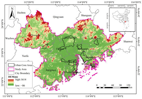
Figure 1.
Location of the GBA, China.
2.2. Data Sources and Preprocessing
2.2.1. Remote Sensing Data and Preprocessing
This study utilizes Landsat series remote sensing images provided by NASA (https://images.nasa.gov/, accessed on 10 May 2021) as the primary data source. Landsat-5 TM images were selected for the years 1990, 2000, and 2010, while Landsat-8 OLI images were used for 2020. Given the long acquisition cycle of Landsat data and the frequent cloud cover in the GBA, this study modified the conventional approach of selecting a single cloud-free or minimally clouded image from the target year. Instead, images were selected from the target year and the adjacent years within the vegetation growth period (September, October) and the non-growth period (December, January), ensuring cloud coverage below 30%. Data preprocessing included cloud removal and water masking. Cloud removal was performed using the CFMASK algorithm based on the QA quality assessment band of Landsat images. Additionally, permanent water bodies, including rivers and reservoirs, were masked using the secondary wetland category from the 1990–2020 land cover product of the Greater Bay Area [49] to minimize the impact of surface water on the humidity principal component load.
2.2.2. Impact Factor Data and Preprocessing
The driving factors influencing the distribution and evolution of ecological quality can be categorized into natural and anthropogenic factors. Based on previous studies [50,51,52,53] and data availability, this study selects four natural factors—temperature, precipitation, elevation, and slope—and four anthropogenic factors—land use type, population density, GDP, and nighttime light index. The primary data sources and details are listed in Table 1. Since nighttime light and GDP data for 1990 are unavailable, this study substitutes them with data for 1992.

Table 1.
Main information and sources of impact factor data.
The preprocessing of driving factor data was conducted primarily using ArcGIS 10.2. Due to inconsistencies in spatial extent and projection among different datasets, all data were first clipped and reprojected to align with the study area. Additionally, considering variations in spatial resolution, all datasets were resampled to a uniform resolution of 1 km × 1 km.
Since the geographical detector model used in the subsequent analysis requires categorical variables, the independent variables were reclassified. Land use type data were classified into six categories based on product specifications, while other numerical driving factors were discretized into five categories using the natural breaks method in ArcGIS.
2.3. Constrcution of the URSEI
2.3.1. Indicator Factors
The Remote Sensing Ecological Index (RSEI) model integrates four key indicator factors closely related to human daily life: greenness, humidity, heat, and dryness. Specifically, the Normalized Difference Vegetation Index (NDVI) represents the greenness indicator, the humidity component (WET) derived from tasseled cap transformation represents surface moisture, the average synthesis of the Index-Based Built-up Index (IBI) and the Soil Index (SI) serves as the dryness indicator (NDBSI), and the Land Surface Temperature (LST) represents the heat indicator. These four indicators are entirely derived from remote sensing data, making them easily accessible, with a computational process that requires no manual intervention, ensuring objective and reliable results. The Unified Remote Sensing Ecological Index (URSEI) retains the four indicator factors of RSEI, with the calculation methods for each ecological indicator shown in Table 2.
Table 2.
The calculation method of ecological indicators.
2.3.2. Synthesis of Indicator Factors
In this study, multiple images were selected for each monitoring year, necessitating a synthesis process to generate the four indicator factors for each monitoring period. For greenness, humidity, and dryness indicators, a median composite was first applied separately to the vegetation growing season and the non-growing season images, followed by averaging the results from both periods. The median composite effectively reduces the influence of weather conditions, precipitation, and solar altitude angle, minimizing anomalies and ensuring that the indicators accurately reflect the average conditions of each period. This approach prevents extreme observations from skewing the overall assessment. The final averaging process provides a more comprehensive representation of the ecological conditions throughout the year, mitigating potential biases from single-period observations and delivering a more stable and integrated ecological evaluation.
where represents the indicator factor, denotes the year, represents the vegetation growing season, represents the non-growing season, denotes the median operator, and represents the indicator on date of year .
For the heat indicator, imagery from the autumn vegetation growing season is selected for each monitoring period. The Landsat thermal infrared data from path/row 122/44 at the center of the study area is used as the reference. A random forest regression model is applied to calibrate the thermal infrared data from other path/row numbers using overlapping areas, generating temperature-consistent thermal infrared data aligned with the reference (122/44). A median operator is then used to synthesize the thermal infrared data for the entire GBA. In the random forest regression model, input variables include land cover type, elevation, slope, NDVI, NDWI, WET, IBI, and SI.
2.3.3. Indicator Normalization Based on Invariant Regions
The RSEI model employs range normalization to eliminate dimensional differences among indicators. In existing studies, normalization is typically performed separately for each time period by applying the minimum and maximum values from individual datasets to normalize corresponding indicators. However, this method is susceptible to extreme values, which may introduce biases in the results. Over the past 30 years, the Greater Bay Area has undergone significant urban expansion and ecological changes, leading to substantial differences in the statistical distribution of ecological indicators. While conventional probability-based normalization methods (such as Z-score or Gaussian normalization) can adjust data distribution, they may reduce time-series consistency, affecting the spatial-temporal comparability of indicators and the accuracy of evolution pattern analysis.
To address the issue of indicator normalization, this study proposes an invariant-region-based normalization method. First, using land cover classification data of the Greater Bay Area from 1990 to 2020 [49], a pixel-by-pixel comparison method was applied to identify areas with unchanged land cover types. To accurately delineate long-term stable land cover regions, three decadal intervals (1990–2000, 2000–2010, and 2010–2020) were established to generate stable land cover layers for each period. Finally, spatial intersection analysis was performed to extract areas where land cover types remained unchanged over the entire 30-year period. The formula is as follows:
, , and represent the land cover layers for the periods 1990–2000, 2000–2010, and 2010–2020, where no changes in land cover occurred; represents the intersection of the three invariant region layers.
Then, based on the invariant layer , the indicator factors for different monitoring periods are masked. The cumulative probability distribution function method is applied to calculate the 1st and 99th percentiles of the masked indicators, which are used as the minimum and maximum values. Finally, these statistical results are used to normalize the original, non-masked indicator factors, ensuring that their range is constrained between 0 and 1. At the same time, dryness and heat are treated as negative indicators and undergo reverse normalization to ensure that the negative indicators are reasonably reflected in the overall ecological assessment.
2.3.4. Multi-Temporal Fusion Principal Component Analysis
The RSEI model uses principal component analysis (PCA) to construct a composite ecological index for each monitoring period and standardizes the RSEI values to a range of 0–1 using range normalization, effectively reflecting the relative ecological condition of a specific spatial region at a given time. However, in areas with significant ecological changes, the RSEI value only represents the relative condition within a specific period, making it difficult to accurately reflect the long-term ecological evolution trend across different years.
In this study, ecological indicator factors from four monitoring periods are fused using a unified principal component analysis to construct a composite ecological index. First, the normalized indicator factors are used as variables, and they are input into PCA synchronously and with equal weight to ensure that the data are processed under the same standard. Then, the contribution rate of the first principal component (PC1) is assessed. If it exceeds 70%, PC1 can be used to create the composite ecological index. Unlike the traditional RSEI model, this study does not re-normalize the composite ecological index. Instead, it normalizes the feature vector of PC1 and applies it uniformly to all monitoring periods to generate the Unified Remote Sensing Ecological Index (URSEI), ensuring the comparability of ecological quality changes across different time periods. The formula is as follows:
where is the eigenvector of PC1, satisfying .
2.4. Average Correlation
Average correlation is used in this study to test the applicability of URSEI. A value close to 1 indicates a higher degree of comprehensive representation by the model, signifying stronger applicability. The formula is as follows:
where , , , and represent the correlation coefficients of the , , , and indicators at the same time, and n is the number of indicators.
2.5. Spatial Autocorrelation Analysis
Spatial autocorrelation analysis is used to test whether the attribute values of elements with spatial locations are related to the attribute values at neighboring spatial points. It is an important indicator of the aggregation or dispersion of spatial elements. It includes both global spatial autocorrelation and local spatial autocorrelation [54,55,56,57]. By calculating the global Moran’s I index, it can be used to analyze the overall spatial correlation and spatial differences in the region during different periods. The formula is as follows:
where is the number of samples, and are the attribute values of at spatial locations and , is the average value of attribute , and is the spatial weight matrix. The range of Moran’s I index is (−1, 1). When , it indicates a positive correlation between spatial units; when , it indicates a negative correlation between spatial units; when , it indicates no correlation, representing a random distribution.
The local Moran’s I index can be used to assess the correlation and significance between a region and neighboring regions and to visualize it using the Local Indicators of Spatial Association (LISA). The calculation formula for the local Moran’s I is as follows:
where the meanings of the parameters are the same as in the previous Formula (15).
2.6. Geographical Detector
The geographical detector is a statistical model proposed by Wang Jinfen et al. [39] specifically designed to detect spatial differentiation characteristics and their driving mechanisms. In this study, the eight driving factors from Section 2.2.2 are used as independent variables , with URSEI values as the dependent variable . The factor detector, interaction detector, and risk zone detector in the geographical detector are used to systematically explore the impact and interrelationships of various factors on the spatial differentiation of ecological quality.
(1) Factor detection: This is used to analyze the extent to which the selected independent variables explain the spatial differentiation of the dependent variable (URSEI) at different time stages. Its explanatory power is measured by the -value, as follows:
where represents the stratification of the independent variable , i.e., the number of categories; and are the number of sampling points in the -th category of the independent variable and the total number of sampling points in the region, respectively; and are the variances of the -th category region for the independent variable and the variance of across the entire region, respectively; and the range of is from 0 to 1. The larger the value, the stronger the explanatory power of the independent variable on the dependent variable , and vice versa. The value indicates that explains of .
(2) Interaction detection: This is used to identify the interactions between different influencing factors and assess how the explanatory power of the dependent variable changes when two factors (such as and ) act together. The interactions between factors can be divided into five types, and their corresponding -value ranges are shown in Table 3.
Table 3.
Interaction types of the detection factors.
(3) Risk zone detection: This is used to evaluate whether there is a significant difference in the mean of the dependent variable between any two sub-regions within the different strata of the independent variable , and to conduct significance testing using the -statistic.
where is the mean URSEI value in region , is the sample size within the sub-region, and represents variance.
3. Results
3.1. Model Validation
Table 4 presents the principal component analysis results for the four monitoring periods from 1990 to 2020 and the fused data, including the eigenvalue and contribution rate of the first principal component (PC1), as well as the corresponding eigenvectors for each indicator factor in PC1. As shown in Table 4, the contribution rate of PC1 exceeds 75% for each period, and for the fused and unified principal component analysis result, the contribution rate of PC1 reaches 81.6%. This indicates that PC1 integrates the majority of the characteristics of the four indicator factors and can be used to create the comprehensive ecological index. The feature vector of the unified fusion shows that the PC1 weights for NDVI, WET, NDBSI, and LST are 0.612, 0.425, 0.525, and 0.413, respectively. Since the negative indicators NDBSI and LST have been reverse normalized, their eigenvectors are positive values.
Table 4.
The result of principal component analysis.
The correlation coefficients between each indicator and the average correlation between the URSEI and the individual indicators were calculated. The results are shown in Table 5, where all correlation coefficients pass the significance test at the 99% confidence level. The average correlation between the URSEI and the ecological indicators for the four monitoring periods from 1990 to 2020 is 0.763, 0.733, 0.791, and 0.812, respectively, indicating that the URSEI is a reasonable comprehensive ecological quality assessment metric. Furthermore, in all four monitoring periods, the average correlation of the URSEI is higher than that of any single ecological indicator, demonstrating that the URSEI is more suitable for evaluating ecological quality than individual indicators.
Table 5.
Correlation matrix among the URSEI and four indicators.
3.2. Spatiotemporal Changes in Ecological Quality
To better quantify and visualize the URSEI, this study follows literature [17] and classifies the URSEI values into five levels at intervals of 0.2: [0–0.2), [0.2–0.4), [0.4–0.6), [0.6–0.8), and [0.8–1], representing poor, relatively poor, moderate, good, and excellent ecological quality, respectively. The classification maps of ecological quality in the GBA from 1990 to 2020 are shown in Figure 2.
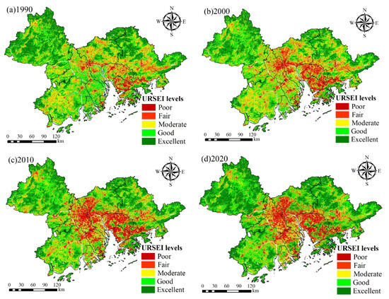
Figure 2.
Spatial distribution of the URSEI in the GBA from 1990 to 2020.
From 1990 to 2020, the spatial heterogeneity of ecological quality across the GBA was high, with significantly lower ecological quality in urban areas compared to non-urban areas. Over the 30-year period, ecological quality exhibited substantial changes with notable temporal variations. In 1990, areas classified as “poor” in ecological quality were relatively scattered, aligning with the geographic locations of built-up urban areas across the GBA, forming a distinct multi-center distribution pattern. Meanwhile, areas classified as “excellent” were mainly concentrated in the northeastern and northwestern parts of the GBA. By 2000, the extent of areas classified as “poor” had increased significantly compared to 1990, with major expansions occurring in Guangzhou, Dongguan, and Shenzhen along the eastern Pearl River estuary, as well as in Foshan, which is adjacent to Guangzhou. By 2010, the overall ecological quality of the GBA had further deteriorated, with a more pronounced spatial clustering of areas classified as “poor” in the central region. However, by 2020, the rate of ecological quality decline had slowed, with “poor” ecological quality areas remaining largely unchanged. At the same time, areas classified as “excellent” had significantly expanded in the northwestern and northeastern parts of the GBA.
Based on the URSEI classification results, the proportion of pixels in different ecological quality levels across the GBA from 1990 to 2020 was calculated, along with the mean URSEI values for the four monitoring periods. The results are shown in Figure 3. Over the past 30 years, the proportion of different URSEI levels has undergone varying degrees of change, with the overall mean URSEI showing a “decline-then-rise” trend. The mean URSEI values for the four years were 0.65, 0.60, 0.60, and 0.63, respectively, decreasing from 0.65 in 1990 to 0.63 in 2020. Compared to 1990, the ecological quality of the GBA in 2020 showed a slight decline. The proportions of areas classified as “excellent” and “good” remained relatively stable, while the proportion of “moderate” areas declined significantly. In contrast, the proportions of “poor” and “relatively poor” areas both increased, with the “poor” category rising notably from 2.54% in 1990 to 8.09% in 2020.
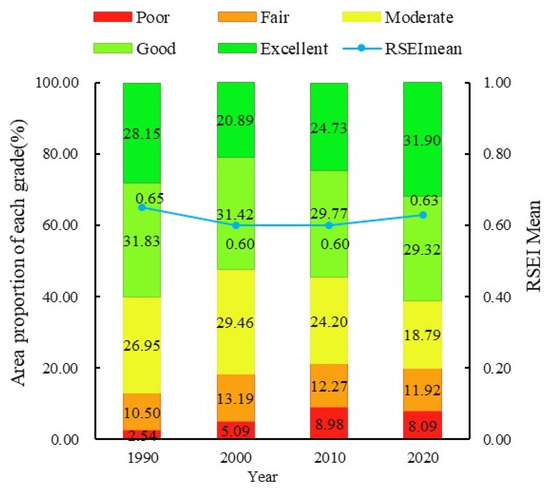
Figure 3.
The proportion of area classified by ecological quality.
Based on the statistical analysis of the proportion of different ecological quality levels over each period, this study analyzed the ecological quality transitions in the GBA from 1990 to 2020 using transfer pathways (Figure 4). The results indicate that most ecological quality changes occurred between adjacent levels, exhibiting a gradual transition pattern where ecological quality progressively shifted from one level to the next. However, it is also important to note that some changes involved abrupt transitions across multiple levels, leading to significant ecological degradation. Examples include transitions from “moderate” to “poor”, “good” to “poor”, and “excellent” to “relatively poor”. These areas require particular attention, and efforts should be intensified to strengthen ecological protection and environmental management. This is crucial to mitigating the immense pressure that economic and urbanization developments impose on the ecological environment.
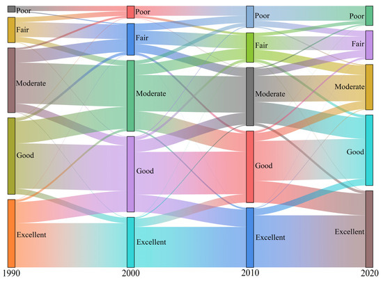
Figure 4.
URSEI transfer matrix for the GBA, 1990–2020.
3.3. Ecological Quality Change Detection
To further analyze the spatial and temporal distribution of ecological quality changes, this study applied a differencing method to detect variations in the URSEI across multiple monitoring periods, using its five classification levels (Table 6).
Table 6.
Transfer matrix of ecological quality levels.
Table 7 and Figure 5 present the change detection results. From 1990 to 2000, the ecological quality of the GBA showed a declining trend, with a degradation area of 15,421.23 km2, accounting for 28.61% of the total area. The spatial distribution of degradation was relatively uniform, affecting every city to varying degrees. Meanwhile, the proportion of improvement was only 8.78%, covering an area of 4730.75 km2. Between 2000 and 2010, ecological quality exhibited a more balanced trend, with the improvement area reaching 11,386.52 km2 (21.13%) and the degradation area covering 10,533.77 km2 (19.55%). The degradation zones were primarily concentrated in Guangzhou, Foshan, Dongguan, Shenzhen, and most parts of Zhongshan. From 2010 to 2020, ecological quality significantly improved, with an improvement area of 14,489.22 km2, accounting for 26.89% of the total. The improvements were distributed across all cities, while the proportion of degraded areas dropped to 12.13%, mainly concentrated in the central region. Over the entire 30-year period (1990–2020), a total of 13,961.27 km2 (25.95%) experienced ecological degradation. The most severe declines occurred in Guangzhou, Foshan, Zhongshan, Dongguan, and Zhuhai, while Zhaoqing, Huizhou, Jiangmen, and Shenzhen also exhibited varying degrees of degradation.
Table 7.
Ecological quality level transfer matrix of in the GBA from 1990 to 2020.
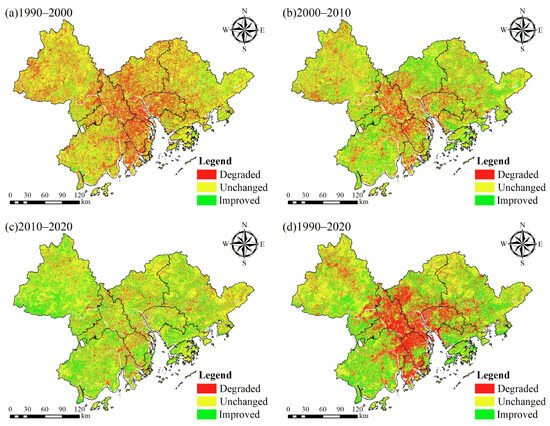
Figure 5.
Change detection of ecological quality in the GBA from 1990 to 2020.
3.4. Ecological Quality Spatial Autocorrelation Analysis
To further explore the spatial aggregation characteristics of ecological quality in the GBA, this study adopts a 5 km × 5 km grid to sample the URSEI values of each period and uses GeoDa software 1.14.0 to conduct spatial correlation analysis on the sampling results.
Global spatial autocorrelation shows (Table 8) that the Moran’s I values of the GBA for all four periods are positive, and the significance test p-values are all less than 0.01, indicating that the ecological quality in the study area has a significant positive spatial autocorrelation feature, meaning regions with good or poor ecological quality tend to be spatially clustered. Among them, the Moran’s I value for 2020 is the highest at 0.614, indicating the strongest spatial clustering of the ecological index in the GBA in 2020. Over the study period, the Moran’s I value shows a gradual increasing trend over time.
Table 8.
Global Moran’s I value of ecological quality at different times in the GBA.
In order to further investigate the specific locations where the ecological quality in the GBA shows spatial aggregation characteristics, local spatial autocorrelation analysis was conducted to generate LISA clustering maps, which were used to analyze the clustering phenomenon of the URSEI values in the study area. As shown in Figure 6, the high–high cluster areas show a clear high-value aggregation feature, and with the passage of time, the area of these clusters has increased. The high–high cluster areas are mainly distributed in the northwest in Zhaoqing City and in the northeast in Guangzhou and Huizhou Cities. These areas are mostly high-altitude regions, with contiguous forest development, high forest cover, minimal human socio-economic activities, low disturbance and damage to the ecological environment, and thus maintain a good ecological quality foundation with high protection levels, exhibiting well-preserved characteristics. The low–low cluster areas have also shown a clear increasing trend over the past 30 years, primarily located in central Guangzhou, Foshan, Dongguan, Shenzhen, and Zhongshan. In these areas, population density is high, urbanization levels are advanced, and land types are mainly built-up areas, where human activities intensively affect the ecological environment, leading to poor ecological quality. Overall, except for the insignificant regions, the high–high and low–low clustered areas of the four periods have relatively large and concentrated areas, while the high–low and low–high clustered areas are smaller and more dispersed in distribution.
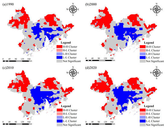
Figure 6.
Locally autocorrelated LISA cluster map of ecological index in the GBA.
3.5. Ecological Quality Driving Factors Analysis
3.5.1. Single Factor Detection Results Analysis
The results of the single factor detection are shown in Table 9. The significance test p-values of all factors are less than 0.001, indicating that the selected independent variables significantly impact the spatial differentiation of ecological quality in the GBA.
Table 9.
The result of single detection from 1990 to 2020.
From the average q-values of the factors for the four monitoring years, nighttime lighting, GDP, and temperature exhibit a strong explanatory power for the spatial differentiation of ecological quality, with average q-values of 0.334, 0.305, and 0.302, respectively, all exceeding 0.3. This suggests that these factors play a dominant role in the spatial differentiation of ecological quality. The next most important factors are elevation, land use type, population density, and slope, with average q-values ranging from 0.2 to 0.3, indicating a moderate explanatory power for URSEI spatial differentiation. Precipitation has the weakest influence, with an average q-value of only 0.042.
From a temporal perspective, the q-values of the factors fluctuate dynamically, and the relative importance of some factors has significantly changed. In 1990, land use type had a relatively weak explanatory power for ecological spatial heterogeneity, with a q-value of 0.145, ranking seventh. However, by 2020, the q-value increased to 0.328, rising to third place. In 1990, temperature was the dominant factor influencing ecological quality spatial differentiation, while in 2000, 2010, and 2020, the nighttime lighting index became the primary influencing factor, indicating that the dominant factors of ecological quality spatial differentiation in the Greater Bay Area shifted from natural to human factors.
Overall, the spatial differentiation of ecological quality in the GBA is influenced by both natural and human factors. In the early stages of the study period, natural factors had a stronger influence on ecological quality spatial differentiation, while in the later stages, human factors had a greater impact than natural factors, reflecting the profound impact of the rapid urbanization process in the GBA on the ecological environment.
3.5.2. Interaction Detection Results Analysis
An interaction detection analysis was conducted on the influencing factors, and the results are shown in Figure 7. Except for the interaction between precipitation and temperature in 1990 and the nonlinear enhancement effects of precipitation interacting with elevation, land use type, and population density in 2020, all other factor interactions exhibited a bivariate enhancement effect. This indicates that the spatial differentiation of ecological quality in the GBA is not the direct, independent result of a single factor but is instead driven by the synergistic enhancement effect of factor interactions.
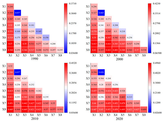
Figure 7.
Interactive detection results of driving factors of ecological quality. Note: X1: (temperature), X2: (precipitation), X3: (DEM), X4: (slope), X5: (type of land use), X6: (population density), X7: (GDP), X8: (nighttime lights).
From 1990 to 2020, the highest-ranked interactions in terms of q-value were as follows: temperature ∩ GDP (0.370) in 1990, nighttime light index ∩ elevation (0.422) in 2000, temperature ∩ GDP (0.451) in 2010, and nighttime light ∩ land use type (0.495) in 2020. Over the 30-year period, the interaction q-value steadily increased from 0.370 to 0.495. Before 2010, interactions between natural and human factors had a more pronounced impact on ecological quality. However, in 2020, interactions among human factors had the greatest influence, reflecting the increasing role of socio-economic development and human activities in ecological quality changes.
By combining these findings with the single-factor detection results, it becomes evident that although precipitation had weak explanatory power when acting alone, its q-value increased significantly when interacting with other factors. This suggests that under the influence of factor interactions, single factors with initially low explanatory power can be significantly enhanced through synergistic effects, improving their ability to explain spatial differentiation in ecological quality.
3.5.3. Risk Zone Detection Analysis
Risk zone detection is used to determine whether there are significant differences in the mean attribute values of different partitions of each factor. In this study, the risk zone detection method was applied to identify the optimal range for quantitative factors and the most suitable type for qualitative factors affecting the URSEI. The 2020 risk detection results were selected as an example for analysis.
As shown in Table 10, the 2020 risk detection results indicate a significant negative correlation between the intensity of human factors and the URSEI mean value. Specifically, the three human-related factors—population density, GDP, and nighttime light index—were classified into five levels, with Level 1 representing the lowest value range and Level 5 representing the highest. The analysis results show that for all three factors, the highest URSEI mean values appeared in Level 1, with values of 0.698 (population density), 0.739 (GDP), and 0.8 (nighttime light index). Their optimal ranges were further determined to be 73–1466 people/km2, 0.04–12.05 million CNY/km2, and 0–19, respectively. These findings suggest that human activities have a significant impact on the ecological quality of the Guangdong-Hong Kong-Macau Greater Bay Area, with lower human activity intensity corresponding to higher URSEI values, indicating better ecological quality. Additionally, when the land use type was forest, the URSEI mean value was the highest, highlighting the crucial role of forest ecosystems in maintaining high ecological quality.
Table 10.
The appropriate type and range of factors.
Among natural factors, each variable was similarly classified into five levels (Level 1: lowest, Level 5: highest). temperature also exhibited a negative correlation with the URSEI, with the highest URSEI mean value occurring at Temperature Level 1 (15.52–19.74 °C), suggesting that areas with lower temperatures tend to have better ecological quality. In terms of elevation and slope classifications, the highest URSEI mean values appeared in Level 4 and Level 5, respectively, indicating that regions with high elevations and steep slopes tend to have better ecological quality, possibly due to lower human disturbance. The precipitation classification results show that the highest URSEI mean value (0.703) was found in Level 5, corresponding to a precipitation range of 1930–2116 mm, suggesting that higher precipitation levels may contribute to maintaining ecological conditions.
4. Discussion
4.1. Applicability Analysis of the URSEI Model
The RSEI has been widely used due to its easy data acquisition, simple calculation, and the absence of manually assigned weights and thresholds. However, when applying the RSEI for long-term ecological quality assessments, the consistency and comparability of time-series evaluation results are often affected by factors such as data acquisition time and weather variations. Additionally, the multiple normalization processes in the RSEI model make the assessment results more dependent on the relative ecological conditions within the study area. In regions with drastic ecological changes, such as the Guangdong-Hong Kong-Macau Greater Bay Area, this dependence further weakens the consistency and comparability of time-series analysis results.
This study proposed multiple improvements to the Remote Sensing Ecological Index (RSEI) to address the challenge of maintaining temporal consistency in ecological quality assessment for cloudy and rainy regions. Given the persistent cloud cover in the Greater Bay Area, our approach moved beyond reliance on single images by selecting imagery from both growing and non-growing seasons within a three-year window (the target year plus one year before and after). Annual indicator factors were generated through median synthesis followed by averaging, which effectively mitigated the impacts of extreme weather and solar altitude variations while enhancing data stability and representativeness. To address thermal data gaps caused by cloud cover, we employed a random forest model using land cover type, NDVI, and elevation as predictors to reconstruct and correct LST data, ensuring spatial consistency.
In terms of indicator normalization, the traditional RSEI normalizes each temporal dataset independently, making it vulnerable to extreme values and temporal incomparability. Our improved method established a land cover invariant reference layer (1990–2020) and extracted indicator values from these stable areas as global normalization thresholds. This approach simultaneously eliminated extreme value effects and maintained consistent normalization baselines across different time periods. For principal component analysis, the conventional RSEI performs PCA separately for each temporal dataset, resulting in inconsistent weights across periods. Our enhanced method merged indicator factors from all four time periods for unified PCA, generating global eigenvectors. The application of fixed weights across all periods ensured the temporal comparability of the URSEI.
The average correlation test revealed that the URSEI’s correlation with individual indicators was significantly stronger than any single indicator, confirming its superior comprehensive representation capability. Furthermore, the URSEI classification maps of the Greater Bay Area (Figure 2) showed no apparent edge-matching or mosaic artifacts, with highly consistent spatial patterns of ecological quality across time periods, ensuring result coherence and integrity while improving visualization effectiveness. Similarly, the ecological quality change detection maps (Figure 5) exhibited no anomalous regions, with detected changes closely matching actual conditions, demonstrating the URSEI’s effectiveness in maintaining temporal comparability for long-term sequence analysis.
Under the challenging conditions of high cloud cover, frequent rainfall, and rapid ecological changes in the GBA, the URSEI model demonstrates strong applicability and reliability. Its improved normalization method and multi-temporal principal component fusion analysis technique not only enhance the consistency and comparability of ecological quality assessments but also provide robust support for accurately analyzing long-term ecological evolution trends. In future applications, the URSEI model could be extended to other regions exhibiting similar climatic characteristics and ecological dynamics. Particularly suitable candidates include rapidly urbanizing areas such as the Yangtze River Delta urban agglomeration and Chengdu-Chongqing economic zone, which share with the Greater Bay Area both intensive anthropogenic pressures and frequent cloudy/rainy conditions. The model would also prove valuable for monitoring ecological changes in other southeastern coastal regions where persistent cloud cover and precipitation similarly challenge conventional remote sensing assessments of fast-evolving environments.
4.2. Spatiotemporal Evolution Characteristics and Influencing Factors of Ecological Quality in the GBA
Based on the spatiotemporal variation analysis of the URSEI, this study reveals the significant characteristics and driving mechanisms of ecological quality evolution in the GBA over the past 30 years (1990–2020). The results indicate that ecological quality changes in the GBA exhibit distinct phased characteristics, with 2010 serving as a turning point, dividing the evolution into two stages.
In the first stage (1990–2010), the GBA experienced a significant decline in ecological quality. This trend is closely associated with rapid industrialization and urbanization in the region. During this period, cities on the eastern shore of the Pearl River Estuary, such as Guangzhou, Shenzhen, and Dongguan, served as the frontiers of China’s economic reform, where industrial expansion and urban development progressed simultaneously, leading to a substantial increase in human activity intensity. Unregulated land use practices and declining vegetation cover contributed to severe environmental degradation. Between 2000 and 2010, as industrial relocation and upgrading occurred, low-end manufacturing industries gradually shifted to western cities such as Foshan, Jiangmen, and Zhongshan, further exacerbating regional ecological deterioration.
In the second stage (2010–2020), ecological quality in the GBA showed an improving trend. This shift can be attributed to several key factors. First, the pace of urbanization slowed down, and the expansion of industrial land significantly decreased. Second, after 2010, both national and local governments introduced a series of ecological and environmental protection policies, such as the Outline of the Plan for the Reform and Development of the Pearl River Delta Region (2008–2020) and the Guangdong-Hong Kong-Macao Greater Bay Area Development Plan, which explicitly set ecological conservation and green development as key objectives, thereby promoting the implementation of ecological restoration projects. Lastly, the regional industrial system progressively transitioned toward high-tech industries, while traditional high-pollution, high-energy-consumption industries were either phased out or upgraded, effectively reducing industrial pressure on the ecological environment. For instance, cities like Shenzhen vigorously developed high-tech industries and modern service sectors, leading to decreased industrial pollution emissions.
From a spatial perspective, the ecological quality of the GBA exhibits significant spatial heterogeneity. The central urban cluster, including Guangzhou, Foshan, Dongguan, Shenzhen, and Zhongshan, generally shows lower ecological quality due to intensive human activities. In contrast, the northwestern and northeastern regions, such as Zhaoqing and Huizhou, benefit from favorable topographic conditions, high vegetation coverage, and lower human disturbances, maintaining relatively high ecological quality levels. This spatial differentiation pattern is strongly coupled with regional economic development levels and human activity intensity.
Geographical detector analysis results indicate that the spatial differentiation of ecological quality in the GBA is driven by both natural and anthropogenic factors. Among these, nighttime light intensity, GDP, and temperature are the primary drivers of ecological quality variations. From a temporal perspective, human-activity-related factors, such as land use type, population density, GDP, and nighttime light index, have shown an increasing explanatory power for the URSEI over time, while the influence of natural factors has remained relatively stable. This finding confirms the dominant role of human activities in shaping ecological quality changes in the GBA, reflecting the profound impact of rapid urbanization on the region’s ecological landscape.
4.3. Ecological Protection and Sustainable Development Recommendations for theGBA
Based on the assessment results of the URSEI, the ecological quality of the GBA has undergone significant spatiotemporal changes over the past 30 years. Particularly during the rapid urbanization and industrialization processes, some areas have experienced noticeable ecological degradation. To address these challenges and ensure the sustainable development of the regional ecosystem, this study proposes the following ecological protection and sustainability recommendations tailored to the GBA’s regional characteristics:
(1) The northwestern and northeastern parts of the GBA (e.g., Zhaoqing and Huizhou) exhibit high ecological quality and a distinct high–high clustering pattern. These areas are predominantly high-altitude regions with dense forest coverage and minimal human disturbance, serving as crucial ecological barriers for the region. It is recommended to strengthen ecological redline management, strictly control the expansion of construction land to prevent ecological degradation and enhance the protection of nature reserves and ecological function zones to improve the stability and resilience of regional ecosystems.
(2) The central urban cluster (e.g., Guangzhou, Shenzhen, Foshan, Dongguan, and Zhongshan) exhibits relatively low ecological quality due to intensive human activities. It is recommended that these cities optimize land use structure, curb the disorderly expansion of construction land, and increase green spaces and water bodies to enhance the stability and resilience of urban ecosystems. Specific measures include promoting urban greening projects by expanding parks and green areas, strengthening water body protection by restoring and rehabilitating wetland ecosystems, and advocating for green buildings and low-carbon city development to mitigate the urban heat island effect.
(3) In industrially intensive areas such as Foshan and Dongguan, ecological degradation is particularly evident. It is recommended to continue promoting industrial upgrading, phasing out outdated production capacities, reducing industrial pollution, and improving ecological environmental quality. Specific measures include encouraging enterprises to adopt clean production technologies to minimize pollutant emissions, strengthening environmental supervision of industrial parks to ensure compliance with emission standards, and promoting green manufacturing and a circular economy to enhance resource efficiency.
(4) The GBA encompasses multiple cities and administrative regions, making cross-regional cooperation and coordination essential for improving ecological quality. It is recommended that cities strengthen collaborative governance in ecological protection, jointly addressing environmental challenges to ensure the integrity and sustainability of the regional ecosystem. Specific measures include establishing a cross-regional ecological protection coordination mechanism, formulating unified ecological protection policies and standards, enhancing the sharing and monitoring of ecological data to improve the scientific precision of regional environmental management, and promoting an ecological compensation mechanism to balance environmental protection with economic development.
4.4. Limitations and Future Works
This study systematically analyzed the spatiotemporal evolution characteristics and driving mechanisms of ecological quality in the Guangdong-Hong Kong-Macao Greater Bay Area (GBA) from 1990 to 2020 using the Unified Remote Sensing Ecological Index (URSEI) and the geographical detector model. However, several limitations need to be acknowledged, and future improvements are proposed as follows:
Regarding data limitations, due to constraints in historical data availability, the nighttime light and GDP data for 1990 were substituted with data from 1992. While such substitution is common in long-term ecological studies, it may introduce certain biases in the analysis of early-stage driving factors of ecological quality. Future research could employ data interpolation or modeling approaches to optimize the completeness of early-stage data and reduce potential biases caused by direct substitution.
In terms of analytical dimensions, this study primarily relied on remote sensing data and large-scale driving factors for assessment, with relatively insufficient consideration of micro-level socioeconomic elements (e.g., environmental protection investments, specific policy implementation effects, and corporate pollution control measures). Subsequent studies should incorporate field surveys or socioeconomic statistical data to further refine the analysis of driving mechanisms.
5. Conclusions
This study introduces the URSEI as an enhancement of the traditional RSEI. Through optimization of data selection, normalization of invariant region indicators, and multi-temporal principal component analysis, the URSEI effectively addresses the challenges of ecological quality assessment in the cloudy and rainy climate of the GBA. The dynamic monitoring results from 1990 to 2020 show significant improvements in the consistency and spatial visualization of ecological assessments.
The findings reveal that the ecological quality of the GBA exhibits a spatial distribution characterized by lower values in the central region and higher values in the northwest and northeast areas. The URSEI values over the years show a trend of decline followed by improvement, with an overall slight degradation of ecological quality, as evidenced by a 24.29% improvement area and a 25.95% degradation area. The spatial analysis indicates a significant positive spatial autocorrelation, with high–high and low–low clustering patterns dominating, which align with the changes in URSEI grades.
The spatial differentiation of ecological quality is influenced by both natural and anthropogenic factors. Key drivers of spatial variation include nighttime light intensity, GDP, and temperature, with human factors having a stronger impact, which has increased over time. This study underscores the importance of considering both natural and human influences in long-term ecological monitoring and provides a reliable method for assessing ecological quality in regions with varying climatic and environmental conditions.
Author Contributions
Conceptualization, F.S. and C.D.; methodology, H.L. and L.Z.; software, L.W.; validation, F.S., C.D. and H.L.; formal analysis, R.J. and L.Z.; investigation, R.J. and H.L.; resources, J.C. and F.S.; data curation, R.J. and H.L.; writing—original draft preparation, R.J. and H.L.; writing—review and editing, F.S. and C.D.; visualization, R.J. and L.Z.; supervision, L.W. and J.C.; project administration, J.C.; funding acquisition, F.S. and H.L. All authors have read and agreed to the published version of the manuscript.
Funding
This research was funded by the Scientific Research Project of the Ecology Environment Bureau of Shenzhen Municipality, grant number SZDL2023001387, the Fundamental Research Foundation of Shenzhen Technology and Innovation Council, grant number JCYJ20220818101617038, the National Natural Science Foundation of China, grant number 42271353, and the Guangdong Basic and Applied Basic Research Foundation, grant number 2024A1515011858.
Data Availability Statement
The data presented in this study are available within the article.
Conflicts of Interest
The authors declare no conflicts of interest.
References
- Zeng, S.Y.; Ma, J.; Yang, Y.J.; Zhang, S.L.; Liu, G.J.; Chen, F. Spatial assessment of farmland soil pollution and its potential human health risks in China. Sci. Total Environ. 2019, 687, 642–653. [Google Scholar] [CrossRef] [PubMed]
- Mahmoud, S.H.; Gan, T.Y. Impact of anthropogenic climate change and human activities on environment and ecosystem services in arid regions. Sci. Total Environ. 2018, 633, 1329–1344. [Google Scholar] [CrossRef] [PubMed]
- Wang, X.; Lu, B.B.; Li, J.S.; Liu, Q.Y.; He, L.H.; Lv, S.C.; Yu, S.H. Spatio-temporal analysis of ecological service value driven by land use changes: A case study with Danjiangkou, Hubei section. Resour. Environ. Sustain. 2024, 15, 100146. [Google Scholar] [CrossRef]
- Fang, C.L.; Wang, Z.B.; Liu, H.M. Exploration on the theoretical basis and evaluation plan of Beautiful China construction. Acta Geogr. Sin. 2019, 74, 619–632. [Google Scholar]
- Yu, G.R.; Wang, Y.S.; Yang, M. Discussion on the ecological theory and assessment methods of ecosystem quality and its evolution. Chin. J. Appl. Ecol. 2022, 33, 865–877. [Google Scholar]
- Li, J.Q.; Tian, Y. Assessment of Ecological Quality and Analysis of Influencing Factors in Coal-Bearing Hilly Areas of Northern China: An Exploration of Human Mining and Natural Topography. Land 2024, 13, 1067. [Google Scholar] [CrossRef]
- Xu, T.; Wu, H. Spatiotemporal Analysis of Vegetation Cover in Relation to Its Driving Forces in Qinghai-Tibet Plateau. Forests 2023, 14, 1835. [Google Scholar] [CrossRef]
- Wang, R.; Ding, X.; Yi, B.J.; Wang, J.L. Spatiotemporal characteristics of vegetation cover change in the Central Yunnan urban agglomeration from 2000 to 2020 based on Landsat data and its driving factors. Geocarto Int. 2024, 39, 2316643. [Google Scholar] [CrossRef]
- Wang, Y.L.; Zhang, A.; Gao, X.T.; Zhang, W.; Wang, X.H.; Jiao, L.L. Spatial-Temporal Differentiation and Driving Factors of Vegetation Landscape Pattern in Beijing-Tianjin-Hebei Region Based on the ESTARFM Model. Sustainability 2024, 16, 10498. [Google Scholar] [CrossRef]
- Yuan, D.B.; Zhang, L.Y.; Fan, Y.Q.; Sun, W.B.; Fan, D.Q.; Zhao, X.R. Spatio-Temporal Analysis of Surface Urban Heat Island and Canopy Layer Heat Island in Beijing. Appl. Sci. 2024, 14, 5034. [Google Scholar] [CrossRef]
- Chen, X.; Zhang, S.C.; Tian, Z.Y.; Luo, Y.Q.; Deng, J.; Fan, J.H. Differences in urban heat island and its driving factors between central and new urban areas of Wuhan, China. Environ. Sci. Pollut. Res. 2023, 30, 58362–58377. [Google Scholar] [CrossRef]
- Miao, S.; Liu, C.; Qian, B.J.; Miao, Q. Remote sensing-based water quality assessment for urban rivers: A study in linyi development area. Environ. Sci. Pollut. Res. 2020, 27, 34586–34595. [Google Scholar] [CrossRef] [PubMed]
- Zheng, Z.H.; Wu, Z.F.; Chen, Y.B.; Yang, Z.W.; Marinello, F. Exploration of eco-environment and urbanization changes in coastal zones: A case study in China over the past 20 years. Ecol. Indic. 2020, 119, 106847. [Google Scholar] [CrossRef]
- Li, C.; Chen, T.; Jia, K.; Plaza, A. Coupling Analysis Between Ecological Environment Change and Urbanization Process in the Middle Reaches of Yangtze River Urban Agglomeration, China. IEEE J. Sel. Top. Appl. Earth Observ. Remote Sens. 2024, 17, 880–892. [Google Scholar] [CrossRef]
- Wang, C.; Sheng, Q.; Zhu, Z. Exploring Ecological Quality and Its Driving Factors in Diqing Prefecture, China, Based on Annual Remote Sensing Ecological Index and Multi-Source Data. Land 2024, 13, 1499. [Google Scholar] [CrossRef]
- Xu, H.; Wang, Y.; Guan, H.; Shi, T.; Hu, X. Detecting Ecological Changes with a Remote Sensing Based Ecological Index (RSEI) Produced Time Series and Change Vector Analysis. Remote Sens. 2019, 11, 2345. [Google Scholar] [CrossRef]
- Xu, H.Q. A remote sensing index for assessment of regional ecological changes. China Environ. Sci. 2013, 33, 889–897. [Google Scholar]
- Gan, X.T.; Du, X.C.; Duan, C.J.; Peng, L.H. Evaluation of Ecological Environment Quality and Analysis of Influencing Factors in Wuhan City Based on RSEI. Sustainability 2024, 16, 5809. [Google Scholar] [CrossRef]
- Chen, Z.Y.; Chen, R.R.; Guo, Q.; Hu, Y.L. Spatiotemporal Change of Urban Ecologic Environment Quality Based on RSEI-Taking Meizhou City, China as an Example. Sustainability 2022, 14, 13424. [Google Scholar] [CrossRef]
- Zhang, L.; Hou, Q.; Duan, Y.; Ma, S. Spatial and Temporal Heterogeneity of Eco-Environmental Quality in Yanhe Watershed (China) Using the Remote-Sensing-Based Ecological Index (RSEI). Land 2024, 13, 780. [Google Scholar] [CrossRef]
- He, Y.R.; Chen, Y.H.; Zhong, L.; Lai, Y.F.; Kang, Y.T.; Luo, M.; Zhu, Y.F.; Zhang, M. Spatiotemporal evolution of ecological environment quality and its drivers in the Helan Mountain, China. J. Arid Land 2025, 17, 224–244. [Google Scholar] [CrossRef]
- Cai, C.; Li, J.Y.; Wang, Z.Q. Long-Term Ecological and Environmental Quality Assessment Using an Improved Remote-Sensing Ecological Index (IRSEI): A Case Study of Hangzhou City, China. Land 2024, 13, 1152. [Google Scholar] [CrossRef]
- Feng, Z.X.; She, L.; Wang, X.H.; Yang, L.; Yang, C. Spatial and Temporal Variations of Ecological Environment Quality in Ningxia Based on Improved Remote Sensing Ecological Index. Ecol. Environ. Sci. 2024, 33, 131–143. [Google Scholar]
- Cheng, L.L.; Wang, Z.W.; Tian, S.F.; Liu, Y.T.; Sun, M.Y.; Yang, Y.M. Evaluation of eco-environmental quality in Mentougou District of Beijing based on improved remote sensing ecological index. Chin. J. Ecol. 2021, 40, 1177–1185. [Google Scholar]
- Ke, L.N.; Xu, J.H.; Wang, N.; Hou, J.X.; Han, X.; Yin, S.S. Evaluation of Ecological Quality of Coastal Wetland Based on Remote Sensing Ecological Index: A Case Study of Northern Liaodong Bay. Ecol. Environ. Sci. 2022, 31, 1417–1424. [Google Scholar]
- Liu, Y.; Dang, C.Y.; Yue, H.; Lu, C.G.; Qian, J.X.; Zhu, R. Comparison between modified remote sensing ecological index and RSEI. J. Remote Sens. 2022, 26, 683–697. [Google Scholar] [CrossRef]
- Geng, J.; Yu, K.; Xie, Z.; Zhao, G.; Ai, J.; Yang, L.; Yang, H.; Liu, J. Analysis of Spatiotemporal Variation and Drivers of Ecological Quality in Fuzhou Based on RSEI. Remote Sens. 2022, 14, 4900. [Google Scholar] [CrossRef]
- Chen, N.; Cheng, G.; Yang, J.; Ding, H.; He, S. Evaluation of Urban Ecological Environment Quality Based on Improved RSEI and Driving Factors Analysis. Sustainability 2023, 15, 8464. [Google Scholar] [CrossRef]
- Liu, Y.; Zhou, T.; Yu, W. Analysis of Changes in Ecological Environment Quality and Influencing Factors in Chongqing Based on a Remote-Sensing Ecological Index Mode. Land 2024, 13, 227. [Google Scholar] [CrossRef]
- Long, T.; Bai, Z.; Zheng, B. Spatiotemporal Dynamics and Driving Forces of Ecological Environment Quality in Coastal Cities: A Remote Sensing and Land Use Perspective in Changle District, Fuzhou. Land 2024, 13, 1393. [Google Scholar] [CrossRef]
- Yue, H.; Liu, Y.; Li, Y.; Lu, Y. Eco-Environmental Quality Assessment in China’s 35 Major Cities Based On Remote Sensing Ecological Index. IEEE Access 2019, 7, 51295–51311. [Google Scholar] [CrossRef]
- He, Y. Construction of qualitative assessment model of ecological environment quality under river safety remediation. Int. J. Environ. Technol. Manag. 2024, 27, 400–414. [Google Scholar] [CrossRef]
- Wang, J.Y.; Chen, G.; Yuan, Y.R.; Fei, Y.; Xiong, J.N.; Yang, J.W.; Yang, Y.M.; Li, H. Spatiotemporal changes of ecological environment quality and climate drivers in Zoige Plateau. Environ. Monit. Assess. 2023, 195, 912. [Google Scholar] [CrossRef]
- Liu, W.M.; Cheng, Z.Y.; Li, J.; Li, G.; Pan, N.H. Assessment of ecological asset quality and its drivers in Agro-pastoral Ecotone of China. Ecol. Indic. 2025, 170, 113072. [Google Scholar] [CrossRef]
- Zeng, J.W.; Dai, X.; Li, W.Y.; Xu, J.P.; Li, W.L.; Liu, D.S. Quantifying the Impact and Importance of Natural, Economic, and Mining Activities on Environmental Quality Using the PIE-Engine Cloud Platform: A Case Study of Seven Typical Mining Cities in China. Sustainability 2024, 16, 1447. [Google Scholar] [CrossRef]
- Liu, Z.; Wang, S.; Fang, C. Spatiotemporal evolution and influencing mechanism of ecosystem service value in the Guangdong-Hong Kong-Macao Greater Bay Area. J. Geogr. Sci. 2023, 33, 1226–1244. [Google Scholar] [CrossRef]
- Ren, Y.F.; He, X.N.; Jiang, Q.N.; Zhang, F.; Zhang, B.T. Advancing high-quality development in China: Unraveling the dynamics, disparities, and determinants of inclusive green growth at the prefecture level. Ecol. Indic. 2024, 169, 112898. [Google Scholar]
- Pharaoh, E.; Diamond, M.; Jarvie, H.P.; Ormerod, S.J.; Rutt, G.; Vaughan, I.P. Potential drivers of changing ecological conditions in English and Welsh rivers since 1990. Sci. Total Environ. 2024, 946, 174369. [Google Scholar] [CrossRef]
- Wang, J.F.; Xu, C.D. Geodetector: Principle and prospective. Acta Geogr. Sin. 2017, 72, 116–134. [Google Scholar]
- Ju, H.; Zhang, Z.; Zuo, L.; Wang, J.; Zhang, S.; Wang, X.; Zhao, X. Driving forces and their interactions of built-up land expansion based on the geographical detector—A case study of Beijing, China. Int. J. Geogr. Inf. Sci. 2016, 30, 2188–2207. [Google Scholar] [CrossRef]
- Tao, S.; Yi, C.; Weidong, L.; Hui, L. Spatial difference and mechanisms of influence of geo-economy in the border areas of China. J. Geogr. Sci. 2017, 27, 1463–1480. [Google Scholar]
- Zuo, S.; Dai, S.; Song, X.; Xu, C.; Liao, Y.; Chang, W.; Chen, Q.; Li, Y.; Tang, J.; Man, W.; et al. Determining the Mechanisms that Influence the Surface Temperature of Urban Forest Canopies by Combining Remote Sensing Methods, Ground Observations, and Spatial Statistical Models. Remote Sens. 2018, 10, 1814. [Google Scholar] [CrossRef]
- Liang, P.; Yang, X. Landscape spatial patterns in the Maowusu (Mu Us) Sandy Land, northern China and their impact factors. Catena 2016, 145, 321–333. [Google Scholar] [CrossRef]
- Huang, J.; Wang, J.; Bo, Y.; Xu, C.; Hu, M.; Huang, D. Identification of Health Risks of Hand, Foot and Mouth Disease in China Using the Geographical Detector Technique. Int. J. Environ. Res. Public Health 2014, 11, 3407–3423. [Google Scholar] [CrossRef]
- Zhang, H.J. Ecological environment change in Guangdong-Hong Kong-Macao Greater Bay Area based on multi-temporal remote sensing ecological index. Sci. Geogr. Sin. 2019, 8, 8. [Google Scholar]
- Yang, C.; Zhang, C.; Li, Q.; Liu, H.; Gao, W.; Shi, T.; Liu, X.; Wu, G. Rapid urbanization and policy variation greatly drive ecological quality evolution in Guangdong-Hong Kong-Macau Greater Bay Area of China: A remote sensing perspective. Ecol. Indic. 2020, 115, 106373. [Google Scholar] [CrossRef]
- Wu, Y.Y.; Luo, Z.H.; Wu, Z.F. Exploring the Relationship between Urbanization and Vegetation Ecological Quality Changes in the Guangdong-Hong Kong-Macao Greater Bay Area. Land 2024, 13, 1246. [Google Scholar] [CrossRef]
- Wang, Y.; Zhao, Y.H.; Wu, J.S. Dynamic monitoring of long time series of ecological quality in urban agglomerations using Google Earth Engine cloud computing:A case study of the Guangdong-Hong Kong-Macao Greater Bay Area, China. Acta Ecol. Sin. 2020, 40, 8461–8473. [Google Scholar]
- Wu, B.F. ChinaCover; Science Press: Beijing, China, 2017; p. 397. [Google Scholar]
- Liu, J.C.; Xie, T.; Lyu, D.; Cui, L.; Liu, Q.M. Analyzing the Spatiotemporal Dynamics and Driving Forces of Ecological Environment Quality in the Qinling Mountains, China. Sustainability 2024, 16, 3251. [Google Scholar] [CrossRef]
- Ding, X.; Shao, X.; Wang, J.L.; Peng, S.Y.; Shi, J.C. Research on the Spatial-Temporal Pattern Evolution and Driving Force of Ecological Environment Quality in Kunming City Based on Remote Sensing Ecological Environment Index in the Past 25 Years. Pol. J. Environ. Stud. 2024, 33, 1073–1089. [Google Scholar] [CrossRef]
- Wang, X.Y.; Wang, X.D.; Jin, X.; Kou, L.D.; Hou, Y.J. Evaluation and driving force analysis of ecological environment in low mountain and hilly regions based on optimized ecological index. Sci. Rep. 2024, 14, 24570. [Google Scholar] [CrossRef] [PubMed]
- Zhang, S.W.; Wang, Y.; Wang, X.H.; Wu, Y.; Li, C.R.; Zhang, C.; Yin, Y.H. Ecological Quality Evolution and Its Driving Factors in Yunnan Karst Rocky Desertification Areas. Int. J. Environ. Res. Public Health 2022, 19, 16904. [Google Scholar] [CrossRef]
- Zhu, Z.R.; Cao, H.S.; Yang, J.C.; Shang, H.; Ma, J.Q. Ecological environment quality assessment and spatial autocorrelation of northern Shaanxi mining area in China based-on improved remote sensing ecological index. Front. Environ. Sci. 2024, 12, 1325516. [Google Scholar] [CrossRef]
- Wang, S.D.; Si, J.J.; Wang, Y. Study on Evaluation of Ecological Environment Quality and Temporal-Spatial Evolution of Danjiang River Basin (Henan Section). Pol. J. Environ. Stud. 2021, 30, 2353–2367. [Google Scholar] [CrossRef]
- Jiao, K.; Yong, X.Q.; Mao, S.H.; Chen, K.Y. Analysis of the evolution and influencing factors of ecological environment quality after the transformation of resource-exhausted cities based on GEE and RSEI: A case study of Xuzhou City, China. J. Asian Archit. Build. Eng. 2024, 1–19. [Google Scholar] [CrossRef]
- Xia, Q.Q.; Chen, Y.N.; Zhang, X.Q.; Ding, J.L. Spatiotemporal Changes in Ecological Quality and Its Associated Driving Factors in Central Asia. Remote Sens. 2022, 14, 3500. [Google Scholar] [CrossRef]
Disclaimer/Publisher’s Note: The statements, opinions and data contained in all publications are solely those of the individual author(s) and contributor(s) and not of MDPI and/or the editor(s). MDPI and/or the editor(s) disclaim responsibility for any injury to people or property resulting from any ideas, methods, instructions or products referred to in the content. |
© 2025 by the authors. Licensee MDPI, Basel, Switzerland. This article is an open access article distributed under the terms and conditions of the Creative Commons Attribution (CC BY) license (https://creativecommons.org/licenses/by/4.0/).