Article

Automated Global Method to Detect Rapid and Future Urban Areas

by
Heather S. Sussman
* and
Sarah J. Becker
Geospatial Research Laboratory, Engineering Research and Development Center, US Army Corps of Engineers, Alexandria, VA 22315, USA
*
Author to whom correspondence should be addressed.
Land 2025, 14(5), 1061; https://doi.org/10.3390/land14051061
Submission received: 10 April 2025 / Revised: 7 May 2025 / Accepted: 9 May 2025 / Published: 13 May 2025
(This article belongs to the Special Issue Advances in Land Use and Land Cover Mapping (Second Edition))

Abstract

:
As many areas of the world continue to grow, it is important to detect areas that are urbanizing at paces above the norm and predict future urban areas, so that optimal city planning can occur. However, methods to detect rapid urbanization are currently absent. Additionally, methods that predict future urban areas often rely on deep learning algorithms, which can be computationally expensive and require a large data volume. Furthermore, prediction methods are typically developed in a single location and are not evaluated across diverse geographies. In this study, rapid and future urbanization algorithms are developed, which are based on methods that use an ensemble of built-up spectral indices and a random forest classifier to detect built-up land cover in Sentinel-2 imagery, across ten sites that vary in their climate and population. Results show that the rapid urbanization algorithm can highlight anomalous urban growth. The future urbanization algorithm had an average overall accuracy of 0.66 (±0.11) and an average F1-score of 0.46 (±0.23). However, the method performed well in areas without seasonal vegetation changes and bare ground surroundings with overall accuracy values and F1-scores near or over 0.80. Overall, these methods provide an automated global approach to identifying rapid and future urban areas with minimal data and computational resources needed, which can enable urban planners to obtain information quickly so that decision making for city planning can be completed faster.

1. Introduction

More than half of the world’s population lives in cities, and that number is expected to increase [1]. While urban areas tend to be financial and cultural hubs offering many opportunities for work and leisure, those living, working, and sightseeing in urban areas are susceptible to a variety of impacts due to the urban environment itself, and these impacts could be exacerbated as many areas continue to urbanize. One impact of urbanization is the urban heat island (UHI) effect, which refers to how urban areas tend to be warmer than their nearby non-urban surroundings. The main contributor to the UHI phenomenon is the lack of vegetation in cities, which prevents evaporative cooling during the day and leads to higher heat retention by the urban surface at night [2,3]. The UHI effect can increase the risk of heat exhaustion and dehydration [4] and increase energy demands for cooling [5]. Urbanization can also worsen air quality due to more vehicle traffic and factory emissions [6], which can increase the number, and possibly worsen the symptoms, of those with respiratory issues [7]. Additionally, cities can be complex to navigate, which could become more cumbersome with increased infrastructure, and thereby make it difficult to respond to humanitarian emergencies [8]. Furthermore, urbanization can increase the likelihood of conflict as much of the world’s urbanization is occurring in the least developed areas, which could cause crises in food, water, energy, health, and governance [9]. Given that increased urbanization can have numerous impacts, it is necessary to be able to identify areas that are urbanizing at paces above the normal rate and predict future urban areas. This knowledge would support land cover change monitoring and management and aid in urban planning and development.
Prior efforts to map changes in urbanization have used a variety of remote sensing techniques. For example, Tang et al. [10] studied changes in urban land cover in New Delhi, India from 1994 to 2017 using several landscape metrics, including patch size and species diversity. Yuan et al. [11] examined the Twin Cities Metropolitan Area of Minnesota using a hybrid supervised-unsupervised classification method with post-classification refinements on Landsat Thematic Mapper imagery from 1986, 1991, 1998, and 2002 to describe what the land cover type was before changing to urban. These studies and others have focused on documenting the changes in urban land cover, but efforts to map urbanization that is rapid or above normal rates for a given area are absent. An understanding of where urbanization rates are anomalously high is critical so that proper urban planning can be instituted to potentially limit the extent of the possible drawbacks of urbanization.
As many areas continue to urbanize, efforts have been made to develop algorithms that map the predictions of future urban land cover. For example, Markov modeling has been used in several areas to predict future land cover, i.e., Akbar et al. [12] studied Lahore, Pakistan, Hasan et al. [13] studied Bangladesh, and Dadhich and Hanaoka [14] evaluated Jaipur, India. Others have used Cellular Automata (CA), i.e., Han et al. [15] studied Shanghai, China, Tripathy and Kumar [16] evaluated New Delhi, India, and Liu et al. [17] studied the urban area near the Pearl River Delta, China. Several studies have predicted future urban areas by combining the ability of CA to model spatial variation in complex systems with the Markov model’s capacity for long-range prediction [18,19,20]. Others have used machine learning methods, such as the random forest [21] and support vector machine (SVM) [22]. Several studies have also combined machine learning models with other methods, such as CA-Markov modeling [23,24]. Deep learning methods have also been gaining popularity. For example, Wang et al. [25] used the U-Net deep learning algorithm to study urban growth for the North China Plain. While many of these studies achieved fair accuracies when comparing their models to present or past urbanization levels, and thereby the models can be expected to predict future urban areas, one method is not always better than another. For example, the U-Net used by Wang et al. [25] achieved similar accuracy to CA-based models. Yaagoubi et al. [19] also stated that while the Recurrent Neural Network (RNN) deep learning algorithm performed well over Casablanca, Morocco, the accuracy was similar to CA-Markov methods, and the RNN can be complex and demanding due to its numerous operations and required data volume. Therefore, short-term urban growth forecasting may benefit from not using a deep learning approach, especially since there may not be enough satellite images [19]. Deep learning methods can also be computationally expensive; therefore, since deep learning methods may only achieve a slightly higher accuracy than machine learning methods, their usage may not be justified [26]. Additionally, the studies referenced have only tested their methods in a single location, which provides only a case study of how the methods perform. A global approach for future urban mapping is lacking.
Recently, Maloney et al. [27] developed an automated, global method to detect built-up land cover using an ensemble of spectral indices, a new red-band texture layer with Sentinel-2 imagery, and a random forest classifier. Prior to this, early methods to identify built-up land cover used manual delineation [28,29]. However, the early methods are time-intensive and near-real-time monitoring cannot be achieved. Several built-up spectral indices have been developed to map built-up land cover from multispectral data. However, each index has its advantages and disadvantages, such that when used on its own, misclassifications often occur. For example, the Normalized Difference Built-Up Index (NDBI) developed by Zha et al. [30], had several areas of misclassification with barren land in eastern China. Therefore, it is advantageous to take an ensemble approach and use all available built-up spectral indices to identify built-up land cover, as well as develop methods to automate the process [27].
Given the method developed by Maloney et al. [27] has an overall accuracy of 79.95% (±4%) and can quickly identify built-up land cover in any Sentinel-2 scene globally, the opportunity exists to add a temporal component to the method so that it can be used to study urbanization, and specifically to develop components that identify 1) areas that are urbanizing rapidly and 2) potential future urban areas. Therefore, this work expands upon the methods of Maloney et al. [27] by developing a global rapid urbanization metric and future urbanization algorithm based on statistics of the spectral indices and their rates of change.

2. Materials and Methods

2.1. Data

Sentinel-2 Level 2A Bottom of the Atmosphere reflectance imagery was obtained from the Copernicus Browser in which the data are provided publicly by the European Space Agency (ESA, Paris, France). These data were atmospherically corrected by the ESA prior to download for the scattering of air molecules, absorption and scattering effects of atmospheric gases, and absorption and scattering due to aerosol particles. Table 1 shows the Sentinel-2 bands used in this study for the calculation of five built-up spectral indices, a texture layer, and two spectral indices for masking. The Shortwave Infrared (SWIR) band was resampled from 20 m to 10 m using nearest neighbor interpolation to match the resolution of the other bands [27].

2.2. Study Sites

Study sites were selected in a manner that achieved geographic and population variability. To accomplish geographic diversity, two cities from each of the five Köppen Climate Classifications, i.e., tropical, arid, temperate, continental, and polar, were chosen. Within each Köppen Climate Classification category, a large and small city was chosen according to the built-up category definitions used by the United States Army [31], which are shown in Table 2. The one exception to the selection criteria was for the tropical climate category, in which both cities are metropolises. However, these cities have markedly different population densities, i.e., 351.9 persons/km2 for Chon Buri and 6247 persons/km2 for Nairobi. Additionally, these locations had cloud-free imagery, which can be difficult to achieve in tropical locations, and these areas have been noted as cities that are urbanizing quickly [32,33]. The study sites chosen and their respective properties, i.e., Sentinel-2 Granule ID, Sentinel-2 collection dates, Köppen Climate Classification, and built-up category, are shown in Table 3. Sentinel-2 data were obtained for 2018 and 2022 so that temporal trends in urbanization can be calculated. Data were obtained for approximately the same time of year for a given site, and all imagery was required to have <10% cloud cover. A map of the site locations and a snapshot of the Red-Green-Blue (RGB) Sentinel-2 imagery for each site is shown in Figure 1. Additionally, while the methods were developed using 2018 and 2022 Sentinel-2 data, any user of the developed algorithm can change these years, as the only requirement for the algorithm is that two years of Sentinel-2 data are provided.

2.3. Methods

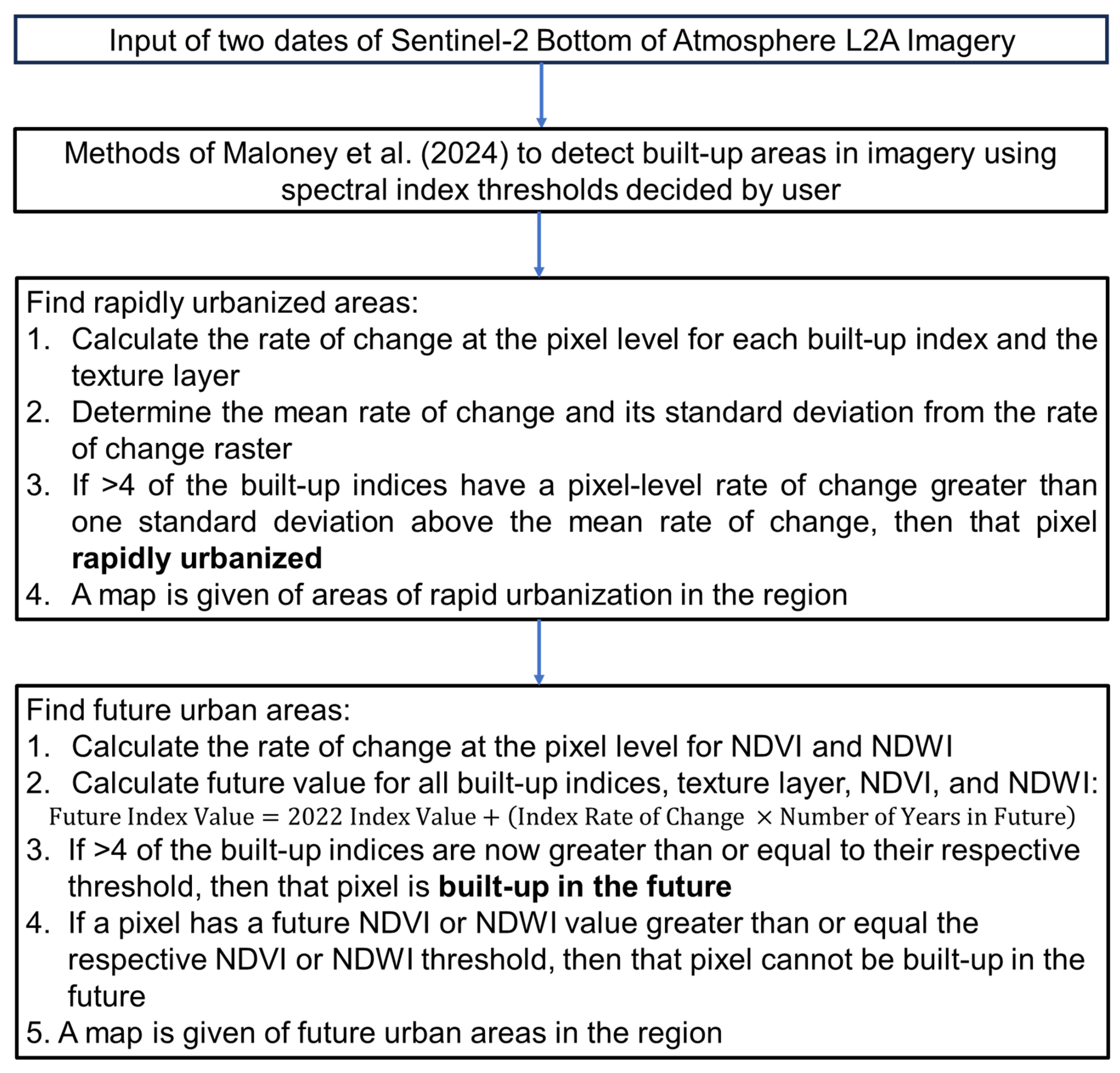
2.3.1. Automated Method for Built-Up Land Cover Identification

Prior to discussing the methods of this study, a brief overview of the methods developed by Maloney et al. [27] will be presented. The reader is referred to the paper for full details. For their methods, one input of Sentinel-2 Level 2A Bottom of the Atmosphere reflectance imagery is required. Five built-up spectral indices are calculated from the Sentinel-2 imagery, which include the (1) Normalized Difference Built-up Index (NDBI), (2) Index-based Built-up Index Adjusted (IBI-adj), (3) Band Ratio for Built-up Area (BRBA), (4) Built-up Area Extraction Index (BAEI), and (5) Visible Blue Band and First Shortwave Infrared Built-up Index (VBI-sh). A texture layer was also developed to identify built-up infrastructure using the red band as this waveband contained high spectral separability between built-up, vegetated, and bare ground areas. The texture layer was calculated by first highlighting value differences using a high-pass filter with a 3 × 3-pixel neighborhood, followed by taking the standard deviation of the output using a 3 × 3-pixel window. Built-up areas were distinguishable by their high standard deviation compared to other land covers. Two spectral indices for masking areas that are not built-up are also calculated from the imagery, which include the (1) Normalized Difference Vegetation Index (NDVI) and (2) Normalized Difference Water Index (NDWI). For the 12 sites that the methods were tested on, site-specific thresholds for the indices were determined that best separated the indices into distinct built-up and not built-up classes, vegetation and not vegetation for NDVI, and water and not water for NDWI. Based on the statistics of these thresholds and which produced the greatest accuracy as measured by the F1-score, the globally optimal threshold for each index was determined (Table 4). The threshold for the texture layer was selected using the Natural Breaks algorithm by sub-setting the output into 10 bins. Using a threshold of bins 6 through 10 produced the highest accuracy in identifying built-up land cover, which represented the areas with the highest standard deviation values.
The algorithm calculates all indices and the texture layer and then reclassifies the rasters into binary classes according to the optimal global thresholds (Table 4). The binary rasters were added together for the 5 built-up indices and texture layer to create an ensemble in which a cell value of ‘6’ indicated that all built-up spectral indices and the texture layer considered that pixel to be built-up. In contrast, a cell value of ‘0’ indicated that all the built-up indices and the texture layer considered the pixel to be not built-up. After these calculations, the ensemble was reclassified to the following: (1) values of ‘0–2’ were classified as not built-up, (2) a value of ‘3’ was classified as potentially confused, and (3) values of ‘4–6’ were classified as built-up. Classifications were additionally corrected by masking with NDWI and NDVI at their respective optimal global thresholds. Additionally, different from Maloney et al. [27] who did not evaluate any polar climate sites, snow masking was applied for the Luleå and Oulu sites using the Sentinel-2 Scene Classification Layer in this study. Equalized stratified random sampling was used to select training data by generating 500 points within the not built-up category and 500 points within the built-up category. The training data were then entered into a random forest classifier to predict a binary classification map of built-up and not built-up categories as the final output. The methods of Maloney et al. [27] used several functions from the ArcPy Spatial Analyst and Management libraries to reclassify rasters and extract unmasked areas, among other functions. These ArcPy libraries were used in the methods of this work as well.

2.3.2. Preliminaries Prior to Algorithm Development

Prior to developing the algorithms to map rapid and future urbanization, several preliminary steps were taken. First, using the data in Table 3, the methods of Maloney et al. [27] were applied. To calculate the accuracy of the methods in identifying built-up land cover in the Sentinel-2 data, equalized stratified random sampling was used to generate 100 built-up and 100 not built-up ground truth points on the binary map output of built-up/not built-up pixel classification for each site and date separately. The ground truth points were compared to the Sentinel-2 RGB composite imagery for accuracy. The overall accuracy (OA) and F1-scores were then calculated. For each site and date, OA and F1-scores were required to be ≥0.80, which would be indicative of high accuracy. A high accuracy is necessary so that the rapid and future urbanization algorithms developed are based on highly accurate built-up land cover identification maps.
Following the accuracy assessment of the original testing data in Table 3, a check on whether accuracy is sensitive to season was assessed. Sentinel-2 data were collected for the opposite season for each site (Table 5). Exceptions occurred for Chon Buri, Nairobi, and Oulu, in which available Sentinel-2 imagery was too cloudy. Accuracy in identifying built-up land cover was assessed in the same manner, i.e., 200 equalized stratified random sampling ground truth points were generated and compared to the Sentinel-2 RGB composite imagery, followed by calculating OA and F1-scores.

2.3.3. Rapid Urbanization Algorithm

To determine areas of rapid urbanization, each built-up spectral index and the texture layer had its rate of change calculated at the pixel level using the 2018 and 2022 Sentinel-2 data in Table 3. Following this, the mean rate of change and standard deviation of the rate of change for each spectral index were calculated for each location individually for the entire Sentinel-2 raster. The pixels that had a mean rate of change that was one standard deviation above the mean rate of change were considered pixels that have rapidly urbanized. Similar to the built-up land cover identification methods [27], if 4 of the 6 built-up indices agreed that a pixel has rapidly urbanized, then that pixel was classified as rapidly urbanized from 2018 to 2022 in the final output. In this manner, areas that are urbanizing rapidly are identified compared to the rate for the particular area of interest.

2.3.4. Future Urbanization Algorithm

To predict future urban areas, the rates of change in NDVI and NDWI were calculated. For NDVI, NDWI, the built-up spectral indices, and the texture layer, the future value is calculated for any number of years in the future that a user of the method is interested in using the 2022 index value and its respective rate of change (Equation (1)).
Future   Index   Value = 2022   Index   Value + Index   Rate   of   Change × Number   of   Years   in   Future
Afterwards, it is determined which pixels have a value that is now greater than or equal to the respective threshold used for each index individually. Similar to previous methods, if 4 of the 6 built-up indices indicate that a pixel is now built-up, then it is classified as a future urban area. However, to provide a check on results, if a pixel has a future NDVI or NDWI value greater than or equal to the respective NDVI or NDWI thresholds, that pixel is masked out in the future urban area output and therefore cannot be classified as built-up.
The future urbanization algorithm was developed by running the methods to predict urban land cover in 2024 using the 2018 and 2022 Sentinel-2 data in Table 3. Sentinel-2 data in 2024 was collected for each site, except for Nairobi and Shōbara in which the data options were too cloudy to use (Table 6). These data are in the same season as the 2018 and 2022 Sentinel-2 data in Table 3 that the methods are developed on. The methods of Maloney et al. [27] were used to identify built-up land cover in 2024 using the 2024 Sentinel-2 data (Table 6), in which the output was compared to the Sentinel-2 RGB 2024 composite using 200 ground truth points generated by equalized stratified random sampling. OA and F1-scores were calculated. Next, the future 2024 urbanization output using the methods of this study was compared to the 2024 Sentinel-2 RGB composite. Similarly, 200 ground truth points were generated by equalized stratified random sampling, which was followed by calculating OA and F1-scores. A flowchart of the methods described is shown in Figure 2.

3. Results

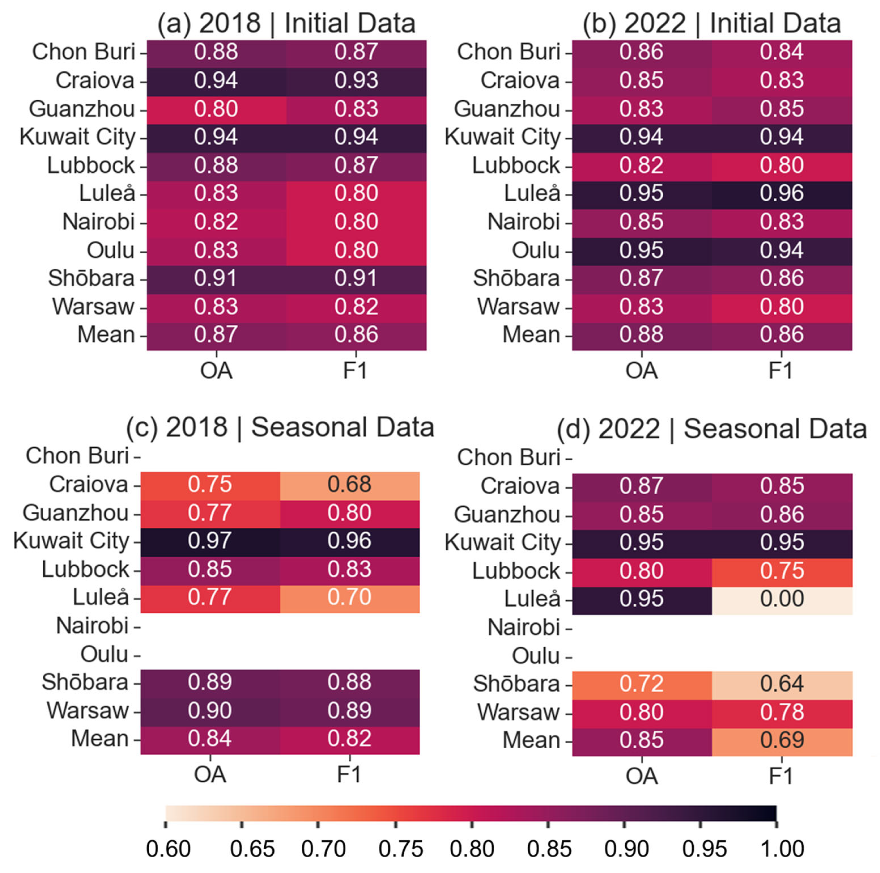
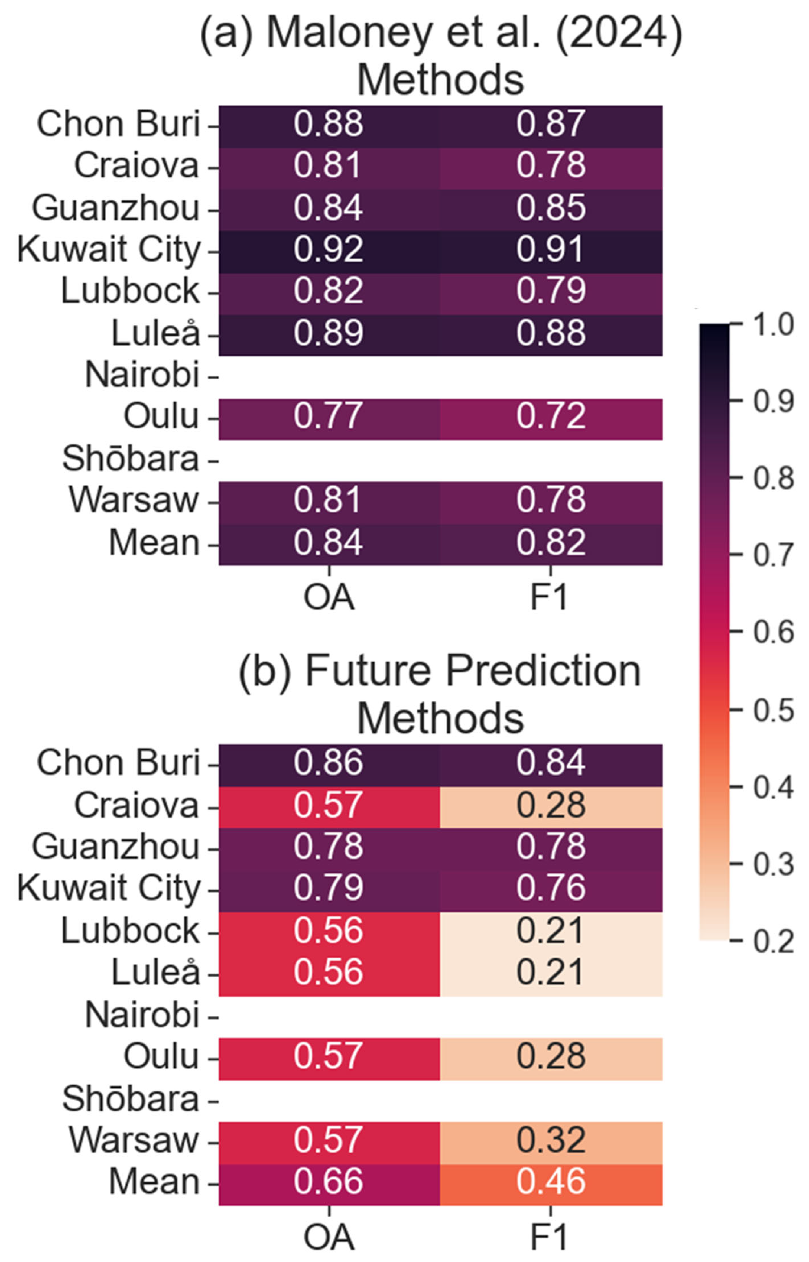
3.1. Accuracy Results

The results of the accuracy assessment using the original data in Table 3 are shown for 2018 in Figure 3a and for 2022 in Figure 3b. Initially, not all sites had OA and F1-scores ≥0.80. For those cases, the spectral index thresholds were adjusted from their optimal global values to be site-specific. When threshold adjustment was necessary, the individual indices were examined using Natural Breaks to determine what value best separated the index into 2 classes, i.e., built/not built-up for built-up indices, vegetation/not vegetation for NDVI, and water/not-water for NDWI. Figure 4 shows an example of this for an area in Kuwait City in 2022 for the BAEI. For the optimal global threshold of 0.31 determined by Maloney et al. [27], the entire area is classified as built-up, which is inaccurate. After applying the Natural Breaks of two bins, the BAEI is best separated into two classes at a value of 0.51, which greatly improves the classification of built-up/not built-up areas (Figure 4). Table 7 shows which indices were adjusted and what the values were adjusted to for all sites. After applying these threshold adjustments when applicable and re-running the methods of Maloney et al. [27], OA and F1-scores were recalculated, and all were ≥0.80 (Figure 3a,b).
The resulting OA and F1-scores for the seasonal comparison test for the sites using the spectral index threshold adjustments from Table 5 are shown for 2018 in Figure 3c and for 2022 in Figure 3d. In general, seasonality does not seem to influence the accuracy of built-up land cover identification since the majority of the OA and F1 values are similar to the contrasting season shown in Figure 3a,b. These results are similar to the findings of Maloney et al. [27]. However, accuracy did fall below 0.80 for the following locations and imagery scenes: (1) Craiova in 2018, Guangzhou in 2018 (OA only), Luleå in 2018 and 2022 (F1 only in 2022), Shōbara in 2022, and Warsaw in 2022 (F1 only). No built-up pixels were identified in 2022 for Luleå, which resulted in an F1-score of 0. Additionally, the high OA of 0.95 for Luleå in 2022 is misleading. The OA was high because nearly all the not built-up points were classified correctly and there were no built-up points to verify. This is inaccurate because built-up land does exist within the Luleå scene.
Overall, while in general, built-up land cover identification is insensitive to season, it may be worthwhile to adjust index thresholds for each site and season. Adjustments of the index thresholds for analysis in a different season may improve accuracy results, especially in areas with distinct seasonal cycles. For the sites in which both OA and F1 were less than 0.80 for the seasonal testing (Figure 3c,d), i.e., Craiova, Luleå, and Shōbara, an investigation on whether changing any of the built-up spectral index thresholds improved accuracy was performed. For Craiova, the BAEI threshold increased from 0.31 to 0.35 and the IBI-adj threshold increased from −0.05 to 0.00. Using the original thresholds, much of the bare vegetation in the early spring season in March was classified as built-up. Bare ground and brown vegetation often can be confused with built-up land cover due to similar spectral properties [27,34,35,36,37,38]. Therefore, by increasing these thresholds, some of the misclassification was removed. Using the new thresholds, the OA and F1-score in 2018 increased from 0.75 and 0.68 in original seasonal testing (Figure 3c) to 0.83 and 0.80, respectively. For 2022, the OA and F1-score became 0.82 and 0.80, which is a slight decrease from the accuracies using the original thresholds, i.e., 0.87 and 0.85 (Figure 3d), but still >0.80 and thus represents high accuracy. Similarly, for Shōbara, much of the bare vegetation was classified as built-up in the fall season in October, so thresholds were again increased. The NDBI threshold increased from −0.08 to 0.00 and the BAEI threshold was increased from 0.31 to 0.39. For 2018, the OA and F1-score both increased to 0.94 from 0.89 and 0.88, and for 2022, the OA and F1-score increased to 0.86 and 0.88 from 0.72 and 0.64, respectively. For Luleå, the BAEI threshold was increased from 0.31 to 0.35 as bare areas were misclassified as built-up in the fall season. For 2018, the OA and F1-score increased to 0.85 and 0.82 from 0.77 and 0.70 (Figure 3c), respectively. For 2022, the OA and F1-score changed to 0.82 and 0.78 from 0.95 and 0.00, respectively. As aforementioned, Luleå in 2022 had no built-up pixels classified correctly as built-up, which resulted in the F1-score of 0.00. However, several areas of bare vegetation were classified as built-up. By increasing the BAEI threshold, many of the bare vegetation misclassifications were removed, and better training data were inputted into the random forest, allowing for more accurate final results. Overall, for areas with strong vegetation cycles, it is likely worthwhile to manipulate thresholds, so that the misclassification of bare vegetation as built-up is minimized. The development of the rapid and future urbanization algorithms was performed on the initial testing data in Table 3 in which index thresholds were adjusted in several cases (Table 7).

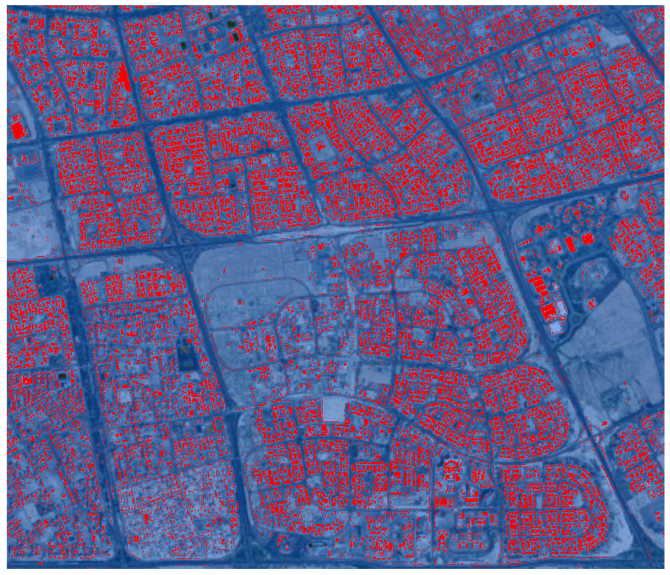
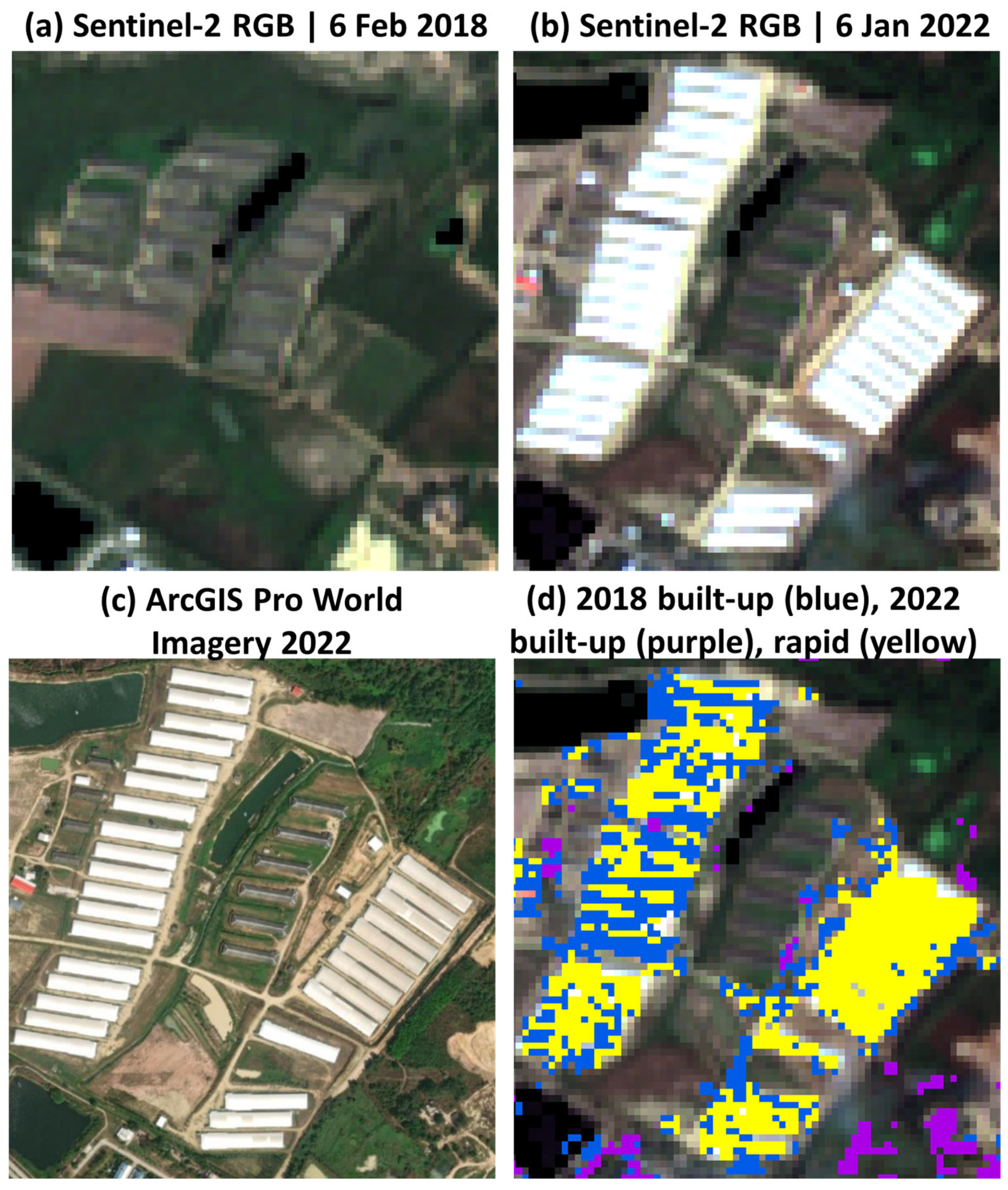
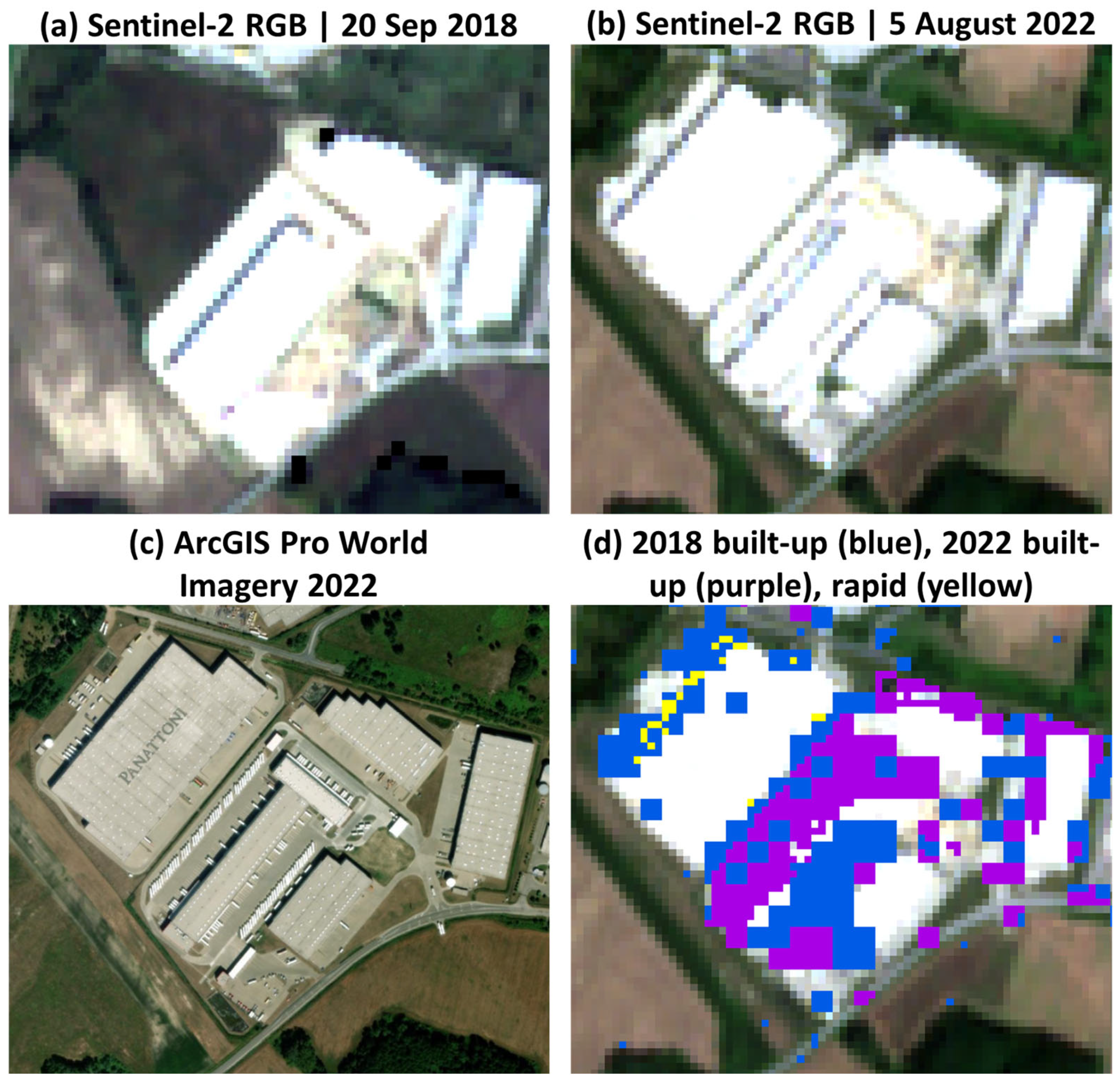
3.2. Rapid Urbanization

Figure 5 shows an example of rapid urbanization output for an area within the Chon Buri, Thailand scene. The rapid urbanization algorithm captured the infrastructure that has been developed in this area. By having this location highlighted as an area experiencing a quick land cover change to urban, it can enable a user of the method to investigate what has developed and why it may have developed quickly. Knowledge of this can aid in land cover monitoring and urban planning.
Figure 6 shows an additional example of rapid urbanization output for an area within the Warsaw, Poland scene. While this example has less rapid urbanization pixels identified compared to Figure 5, it can still enable a user to investigate what has developed in the area. Using the high-resolution Worldview imagery available in ArcGIS Pro (Figure 6c), it is visible that the newly developed building has the word “Panattoni” inscribed on the roof. By using the coordinates of this location, it can be found that this new building, owned by Panattoni, had construction begin in 2019 and finish by the end of that year [39], thus resulting in a quick land cover change to built-up.

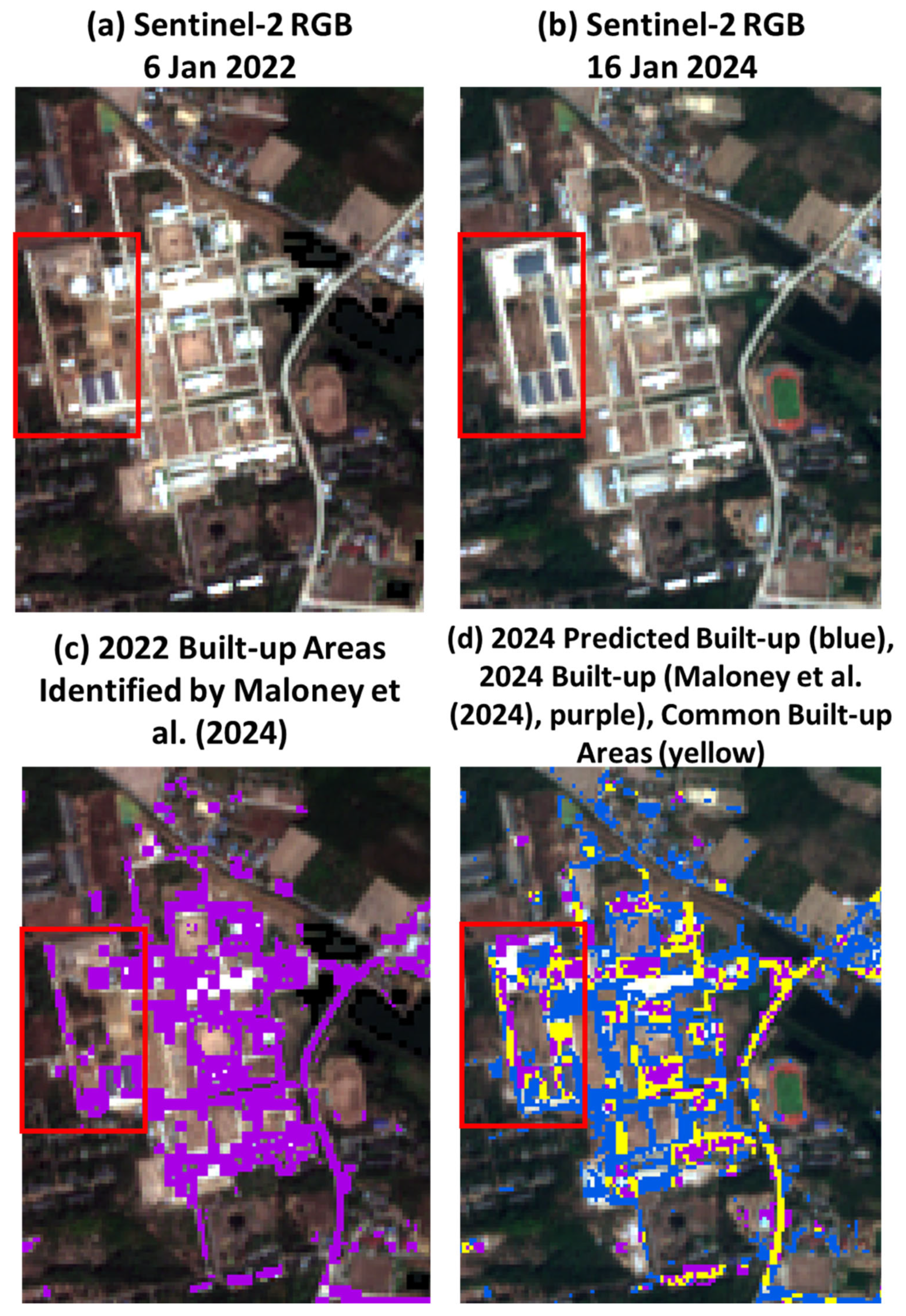
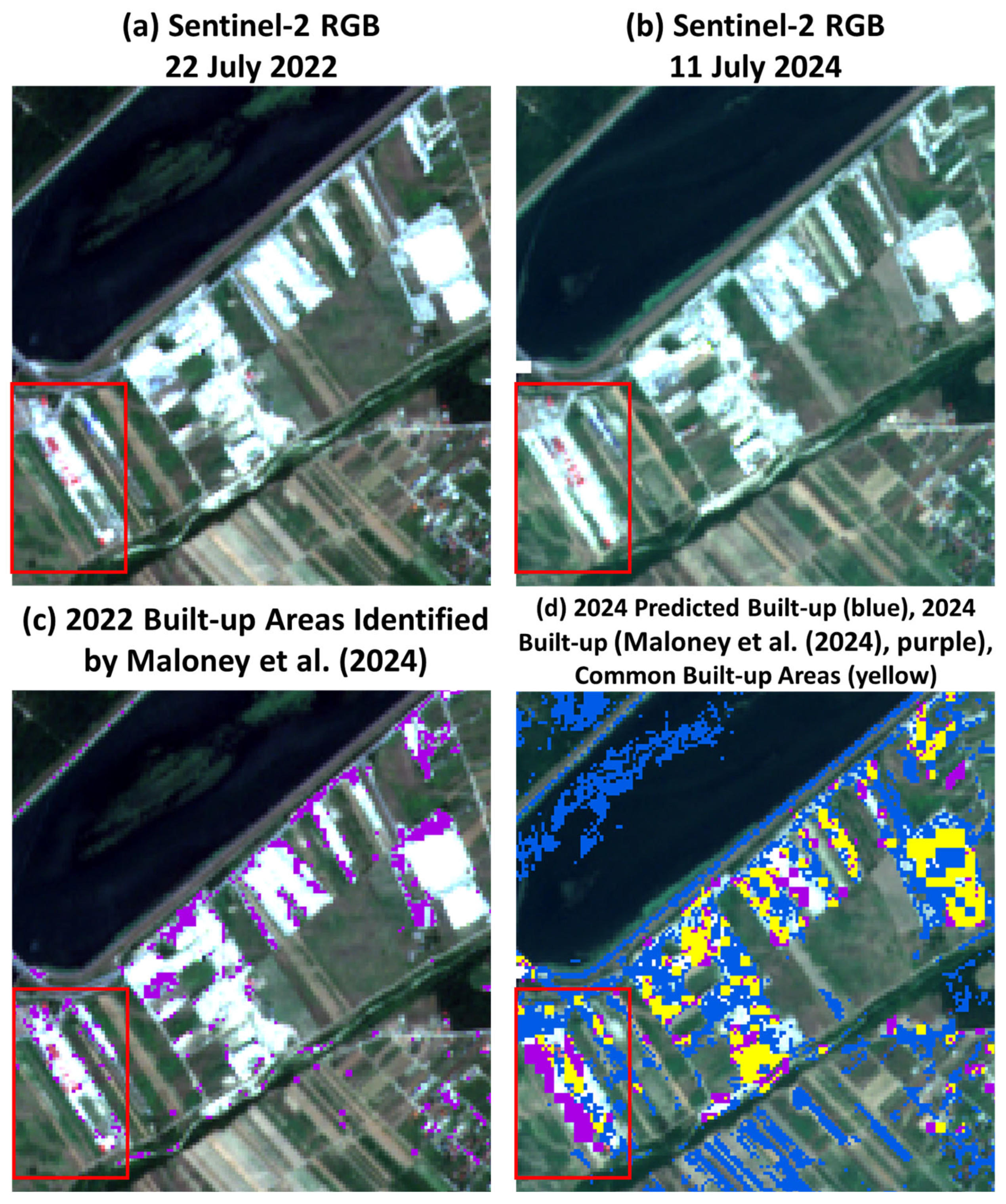
3.3. Future Urbanization

The accuracy results of the methods of Maloney et al. [27] in identifying built-up land cover in 2024 and of the future urbanization algorithm in predicting 2024 built-up land cover, both compared to Sentinel-2 RGB 2024 composite imagery, are shown in Figure 7. The mean OA and F1-score for the Maloney et al. [27] methods were similar, i.e., 0.84 (±0.04) and 0.82 (±0.05), respectively, in which the confidence intervals were determined at the 5% significance level using the Student’s t-test. The mean OA and F1-score for the future urbanization algorithm were different from each other and less than the Maloney et al. [27] methods, i.e., 0.66 (±0.11) and 0.46 (±0.23), respectively. While it is expected that the methods of Maloney et al. [27] will have higher accuracies since the methods calculate the actual built-up land cover in imagery rather than predict built-up land cover, there were several cases in which the accuracies of the future urbanization algorithm were similar to the accuracies of the Maloney et al. [27] method. Notably, for Chon Buri and Guangzhou, the results were comparable between the methods (Figure 7). Consequentially, there can be a degree of confidence in the algorithm for predicting future built-up areas for those sites and possibly similar sites. Figure 8 highlights an example in which the 2024 built-up area identified was similar for both methods for an area in the Chon Buri, Thailand site that experienced urban growth since 2022. For Kuwait City, while the methods of Maloney et al. [27] outperformed the future urbanization algorithm, both OA and F1 were close to 0.80 for the future urbanization algorithm (Figure 7), which also indicates confidence in the algorithm for Kuwait City and possibly similar sites.
The accuracies for the Craiova, Luleå, Oulu, and Warsaw sites using the future urbanization algorithm were all low (Figure 7). For these sites, the surroundings are a mixture of forests and croplands with distinct seasonal cycles. Craiova and Warsaw are both in the continental climate category, and Luleå and Oulu are both in the polar climate category. Many of the forest areas for these sites were classified as future built-up areas. While it is possible that some forest area could have been converted to built-up infrastructure, there was likely an overestimation of built-up land cover by the future urbanization algorithm. Figure 9 shows an example of this overestimation of future built-up land cover for an area in Craiova that experienced urban growth in 2024 compared to 2022. While newly developed areas in 2024 were identified by the future urbanization algorithm, there is an overestimation in which vegetated and bare agricultural areas were classified as built-up despite the imagery clearly showing them as still vegetated or bare fields. This overestimation may be due to the forested areas being dry during the summer season and therefore possibly having brown leaves that are confused as bare ground, which can be misclassified as built-up [30]. The potential misclassification of bare ground as built-up may have also contributed to the bare agricultural fields being identified as built-up. Additionally, some areas of the water body were also identified as built-up despite still appearing as water in the imagery.
The accuracy results using the future urbanization algorithm were also low for the Lubbock site (Figure 7). Croplands and bare ground are the primary land covers in the surroundings of Lubbock. Bare ground is often confused with built-up infrastructure due to similarities in spectral reflectance as often buildings are constructed from local bare ground minerals [34,35,36], which may explain the overestimation of the future built-up area by the algorithm. Figure 10 shows the discrepancies between the methods for an area within Lubbock in which urban growth occurred from 2022 to 2024. While both the methods of Maloney et al. [27] and the future urbanization algorithm picked up the growth within this scene, the future urbanization algorithm also identified many of the bare areas as built-up, which is inaccurate compared to the Sentinel-2 RGB 2024 composite imagery.

4. Discussion and Conclusions

In this study, a temporal component was added to the methods of Maloney et al. [27], which uses an ensemble of spectral indices and a texture layer along with a random forest classifier to identify built-up land cover in any Sentinel-2 scene. The temporal component included here uses two dates of Sentinel-2 imagery to identify areas of rapid urbanization and predict future urban areas. Knowledge of areas that are urbanizing above normal rates and the ability to predict future urban areas can help in land use monitoring and management as well as urban planning and development so that any potential negative impacts of urbanization can be minimized. Prior to this work, there were no methods to identify areas urbanizing above normal rates for a given area. Additionally, nearly all prior future urbanization prediction methods were developed for a single site, and many used deep learning methods, which can be computationally expensive and often have a large data requirement. The methods in this study can be used globally, only need two data files, and do not require heavy computational resources.
Results show that the rapid urbanization algorithm can highlight areas that have urbanized above the normal rate for the location of interest. By pinpointing these areas, a user of the method can then investigate what has been built there and why the area urbanized so quickly. This knowledge could have impacts on urban planning and security for the region.
The future urbanization algorithm performed well for sites without seasonal vegetation cycles and bare ground surroundings, in which OA and F1-scores were near or above 0.80. In the cases where the algorithm performed poorly, there was an overestimation of built-up land cover in which barren and brown vegetated land covers were misclassified as built-up, which can make urban planning challenging in those areas. Built-up and bare/brown vegetation land covers are often confused with each other due to their spectral similarities [38], regardless of the methods used [37,40]. If an area has strong vegetation seasonal cycles, urban planners should apply the methods using data in green vegetation months. Overall, the future urbanization algorithm had an average overall accuracy of 0.66 (±0.11) and an average F1-score of 0.46 (±0.23). Compared to prior studies that developed future urbanization prediction algorithms, the mean accuracy values calculated in this study are generally lower. For example, Yaagoubi et al. [19] achieved an accuracy of 0.95 over Casablanca, Morocco for a deep learning method to predict future urbanization. While this is a high accuracy, the deep learning method comes with the drawback of requiring more data and computational resources. For certain regions, especially areas in the tropics where it is often cloudy, there may not be enough satellite images available to use a deep learning approach. Additionally, not all urban planners may have enough computational resources to run a deep learning model. The method developed in this study may be especially useful in tropical locations due to a small data requirement and the OA and F1-score for tropically located Chon Buri was greater than 0.80. Therefore, the method may perform similarly in other tropical locations. While there are some instances in which the future urbanization algorithm presented here would be useful and achieve fair accuracy in its current form, an opportunity still exists to improve its performance using other remote sensing techniques. Efforts to enhance the algorithm are important so that optimal urban planning and development can be achieved so that the potential drawbacks of urbanization are minimized.
Overall, the methods developed here use remote sensing and machine learning techniques to provide an approach to detect rapid and future urban areas with little computational time and minimal data requirements for any area of the world. Additionally, these methods are the first to use an ensemble of spectral indices to predict future urban land cover. Using an ensemble of spectral indices has been proven to be advantageous in identifying land cover compared to using a single spectral index [27,37,41]. Overall, these methods can support urban planning and land use monitoring globally, particularly for areas with low satellite imagery available and for urban planners without access to high-performance computing. Therefore, these methods are easily accessible and achievable to perform by urban planners. Additionally, since the methods are quick to perform, results are obtained quickly, which can ultimately accelerate the decision-making process for urban planners. Furthermore, for urban planners who have access to high-resolution data and high-performance computational resources, these methods can be used to provide an overview of the large area to then find focus areas that have experienced a high amount of rapid urbanization and/or many future urban areas. By pinpointing the focus areas, high-resolution data and deep learning methods for further study can be used without having to apply data that is time-consuming to process and computationally intensive methods over a large area.

Author Contributions

Conceptualization, H.S.S.; Methodology, H.S.S. and S.J.B.; Validation, H.S.S.; Formal Analysis, H.S.S.; Data Curation, H.S.S.; Writing—Original Draft Preparation, H.S.S.; Writing—Review and Editing, H.S.S. and S.J.B.; Visualization, H.S.S.; Supervision, S.J.B. and H.S.S.; Project Administration, H.S.S. All authors have read and agreed to the published version of the manuscript.

Funding

This research was executed by the U.S. Army Engineer Research and Development Center and supported by the Science Mathematics and Research for Transformation Seed Grant Program under MIPR # HQ0642391795. Permission to publish was granted by the Office of the Technical Director, Geospatial Research Laboratory. The findings of this report are not to be construed as an official Department of the Army position unless so designated by other authorized documents.

Institutional Review Board Statement

Not applicable.

Informed Consent Statement

Not applicable.

Data Availability Statement

The Sentinel-2 data used in this study is available at https://dataspace.copernicus.eu/explore-data/data-collections/sentinel-data/sentinel-2 (accessed on 10 November 2023).

Acknowledgments

The authors thank Laura Clemente for feedback on this manuscript.

Conflicts of Interest

The authors declare no conflicts of interest.

References

  1. Grimm, N.B.; Faeth, S.H.; Golubiewski, N.E.; Redman, C.L.; Wu, J.; Bai, X.; Briggs, J.M. Global change and the ecology of cities. Science 2008, 319, 756–760. [Google Scholar] [CrossRef] [PubMed]
  2. Taha, H. Urban climates and heat islands: Albedo, evapotranspiration, and anthropogenic heat. Energ. Build. 1997, 25, 99–103. [Google Scholar] [CrossRef]
  3. Sussman, H.S.; Dai, A.; Roundy, P.E. The controlling factors of urban heat in Bengaluru, India. Urban Clim. 2021, 38, 100881. [Google Scholar] [CrossRef]
  4. Kovats, R.S.; Hajat, S. Heat stress and public health: A critical review. Annu. Rev. Public Health 2008, 29, 41–55. [Google Scholar] [CrossRef]
  5. Li, X.; Zhou, Y.; Yu, S.; Jia, G.; Li, H.; Li, W. Urban heat island impacts on building energy consumption: A review of approaches and findings. Energy 2019, 174, 407–419. [Google Scholar] [CrossRef]
  6. Wang, Y.; Zhao, T. Impacts of urbanization-related factors on CO2 emissions: Evidence from China’s three regions with varied urbanization levels. Atmos. Pollut. Res. 2018, 9, 15–26. [Google Scholar] [CrossRef]
  7. Heaviside, C.; Macintyre, H.; Vardoulakis, S. The urban heat island: Implications for health in a changing environment. Curr. Environ. Health Rep. 2017, 4, 296–305. [Google Scholar] [CrossRef]
  8. Zetter, R.; Deikun, G. Meeting humanitarian challenges in urban areas. Forced Migr. Rev. 2010, 34, 5–7. Available online: https://library.alnap.org/system/files/content/resource/files/main/zetter-deikun-05-07.pdf (accessed on 3 February 2025).
  9. Kilcullen, D.J. The city as a system: Future conflict and urban resilience. In The Fletcher Forum of World Affairs; The Fletcher Law School of Law and Diplomacy: Medford, MA, USA, 2012; pp. 19–39. Available online: https://www.jstor.org/stable/45289555 (accessed on 3 February 2025).
  10. Tang, J.; Di, L.; Rahman, M.S.; Yu, Z. Spatial-temporal landscape pattern change under rapid urbanization. J. Appl. Remote Sens. 2019, 13, 024503. [Google Scholar] [CrossRef]
  11. Yuan, F.; Sawaya, K.E.; Loeffelholz, B.C.; Bauer, M.E. Land cover classification and change analysis of the Twin Cities (Minnesota) Metropolitan Area by multitemporal Landsat remote sensing. Remote Sens. Environ. 2005, 98, 317–328. [Google Scholar] [CrossRef]
  12. Akbar, T.A.; Hassan, Q.K.; Ishaq, S.; Batool, M.; Butt, H.J.; Jabbar, H. Investigative spatial distribution and modelling of existing and future urban land changes and its impact on urbanization and economy. Remote Sens. 2019, 11, 105. [Google Scholar] [CrossRef]
  13. Hasan, S.; Deng, X.; Li, Z.; Chen, D. Projections of future land use in Bangladesh under the background of baseline, ecological protection and economic development. Sustainability 2017, 9, 505. [Google Scholar] [CrossRef]
  14. Dadhich, P.N.; Hanaoka, S. Remote sensing, GIS and Markov’s method for land use change detection and prediction of Jaipur district. J. Geomat. 2010, 4, 9–15. [Google Scholar]
  15. Han, J.; Hayashi, Y.; Cao, X.; Imura, H. Application of an integrated system dynamics and cellular automata model for urban growth assessment: A case study of Shanghai, China. Landsc. Urban Plan. 2009, 91, 133–141. [Google Scholar] [CrossRef]
  16. Tripathy, P.; Kumar, A. Monitoring and modelling spatio-temporal urban growth of Delhi using cellular automata and geoinformatics. Cities 2019, 90, 52–63. [Google Scholar] [CrossRef]
  17. Liu, Y.; Hu, Y.; Long, S.; Liu, L.; Liu, X. Analysis of the effectiveness of urban-land-use-change models based on the measurement of spatio-temporal, dynamic urban growth: A cellular automata case study. Sustainability 2017, 9, 796. [Google Scholar] [CrossRef]
  18. Baqa, M.F.; Chen, F.; Lu, L.; Qureshi, S.; Tariq, A.; Wang, S.; Jing, L.; Hamza, S.; Li, Q. Monitoring and modeling the patterns and trends of urban growth using urban sprawl matrix and CA-Markov model: A case study of Karachi, Pakistan. Land 2021, 10, 700. [Google Scholar] [CrossRef]
  19. Yaagoubi, R.; Lakber, C.E.; Miky, Y. A comparative analysis on the use of a cellular automata Markov chain versus a convolutional LSTM model in forecasting urban growth using Sentinel 2A images. J. Land Use Sci. 2024, 19, 258–277. [Google Scholar] [CrossRef]
  20. Amir Siddique, M.; Wang, Y.; Xu, N.; Ullah, N.; Zeng, P. The spatiotemporal implications of urbanization for urban heat islands in Beijing: A predictive approach based on CA–Markov modeling (2004–2050). Remote Sens. 2021, 13, 4697. [Google Scholar] [CrossRef]
  21. Frimpong, B.F.; Molkenthin, F. Tracking urban expansion using random forests for the classification of Landsat imagery (1986–2015) and predicting urban/built-up areas for 2025: A study of the Kumasi Metropolis, Ghana. Land 2021, 10, 44. [Google Scholar] [CrossRef]
  22. Karimi, F.; Sultana, S.; Babakan Shirzadi, A.; Suthaharan, S. An enhanced support vector machine model for urban expansion prediction. Comput. Environ. Urban Syst. 2019, 75, 61–75. [Google Scholar] [CrossRef]
  23. Zhou, L.; Dang, X.; Sun, Q.; Wang, S. Multi-scenario simulation of urban land change in Shanghai by random forest and CA-Markov model. Sustain. Cities Soc. 2020, 55, 102045. [Google Scholar] [CrossRef]
  24. Gounaridis, D.; Chorianopoulos, I.; Symeonakis, E.; Koukoulas, S. A random forest-cellular automata modelling approach to explore future land use/cover change in Attica (Greece), under different socio-economic realities and scales. Sci. Total Environ. 2019, 646, 320–335. [Google Scholar] [CrossRef]
  25. Wang, J.; Hadjikakou, M.; Hewitt, R.J.; Bryan, B.A. Simulating large-scale urban land-use patterns and dynamics using the U-Net deep learning architecture. Comput. Environ. Urban Syst. 2022, 97, 101855. [Google Scholar] [CrossRef]
  26. Jozdani, S.E.; Johnson, B.A.; Chen, D. Comparing deep neural networks, ensemble classifiers, and support vector machine algorithms for object-based urban land use/land cover classification. Remote Sens. 2019, 11, 1713. [Google Scholar] [CrossRef]
  27. Maloney, M.C.; Becker, S.J.; Griffin, A.W.H.; Lyon, S.L.; Lasko, K. Automated built-up infrastructure land cover extraction using index ensembles with machine learning, automated training data, and red band texture layers. Remote Sens. 2024, 16, 868. [Google Scholar] [CrossRef]
  28. Slonecker, E.T.; Jennings, D.B.; Garofalo, D. Remote sensing of impervious surfaces: A review. Remote Sens. Rev. 2001, 20, 227–255. [Google Scholar] [CrossRef]
  29. Weng, Q. Remote sensing of impervious surfaces in the urban areas: Requirements, methods, and trends. Remote Sens. Environ. 2012, 117, 34–49. [Google Scholar] [CrossRef]
  30. Zha, Y.; Gao, J.; Ni, S. Use of normalized difference built-up index in automatically mapping urban areas from TM Imagery. Int. J. Remote Sens. 2003, 24, 583–594. [Google Scholar] [CrossRef]
  31. Department of the Army. In Combined Arms Operations in Urban Terrain (FM 3-06.11); Department of the Army: Washington DC, USA, 2002; pp. 1–2. Available online: https://www.bits.de/NRANEU/others/amd-us-archive/fm3-06.11%2802%29.pdf (accessed on 10 February 2025).
  32. World Bank Group. East Asia’s Changing Urban Landscape: Measuring a Decade of Spatial Growth; The World Bank: Washington, DC, USA, 2015; Available online: https://hdl.handle.net/10986/21159 (accessed on 10 February 2025).
  33. Nairobi Swells with Urban Growth. Available online: https://earthobservatory.nasa.gov/images/88822/nairobi-swells-with-urban-growth (accessed on 20 November 2024).
  34. Mahgoub, Y. Globalization and the built environment in Kuwait. Habitat Int. 2004, 28, 505–519. [Google Scholar] [CrossRef]
  35. Rasul, A.; Baltzer, H.; Ibrahim, G.; Hameed, H.; Wheeler, J.; Adamu, B.; Ibrahim, S.; Najmaddin, P. Applying built-up and bare-soil indices from Landsat 8 to cities in dry climates. Land 2018, 7, 81. [Google Scholar] [CrossRef]
  36. Sokienah, Y. Globalization’s impact on the usages of imported and local building materials in Jordan. Int. J. Innov. Technol. Explor. Eng. 2019, 8, 971–975. [Google Scholar] [CrossRef]
  37. Becker, S.J.; Maloney, M.C.; Griffin, A.W.H.; Lasko, K.; Sussman, H.S. Bare ground classification using a spectral index ensemble and machine learning models optimized across 12 international study sites. Geocarto Int. 2025, 40, 1. [Google Scholar] [CrossRef]
  38. Kaur, R.; Pandey, P. A review on spectral indices for built-up area extraction using remote sensing technology. Arab J Geosci 2022, 15, 391. [Google Scholar] [CrossRef]
  39. Panattoni Europe. Available online: https://panattonieurope.com/en-pl/newsroom/panattoni-park-pruszkow-iv-upcoming-speculative-2 (accessed on 23 January 2025).
  40. Langenkamp, J.-P.; Rienow, A. Exploring the Use of Orthophotos in Google Earth Engine for Very High-Resolution Mapping of Impervious Surfaces: A Data Fusion Approach in Wuppertal, Germany. Remote. Sens. 2023, 15, 1818. [Google Scholar] [CrossRef]
  41. Lasko, K.; Maloney, M.C.; Becker, S.J.; Griffin, A.W.H.; Lyon, S.L.; Griffin, S.P. Automated training data Ggeneration from spectral indexes for mapping surface water extent with Sentinel-2 satellite imagery at 10 m and 20 m resolutions. Remote Sens. 2021, 13, 4531. [Google Scholar] [CrossRef]
Figure 1. Map of the ten study sites with a snapshot of their Sentinel-2 RGB composite.
Land 14 01061 g001
Figure 2. A flowchart describing the key steps of the methods to find rapidly urbanized areas and future urban areas.
Land 14 01061 g002
Figure 3. (a) Summary of the OA values and F1-scores for each site using the 2018 Sentinel-2 data in Table 3. The mean OA and F1-score across all sites are both shown. (b) As in (a), but for the 2022 Sentinel-2 data in Table 3. (c) As in (a), but for the 2018 Sentinel-2 data in Table 5 for seasonal testing. (d) As in (a), but for the 2022 Sentinel-2 data in Table 5 for seasonal testing. Blank entries correspond to instances in which no Sentinel-2 imagery was available.
Land 14 01061 g003
Figure 4. The BAEI over a section of the Kuwait City site using Sentinel-2 imagery from 20 May 2022. Built-up areas using the optimal global threshold of 0.31 are shown in blue (i.e., the entire area was identified as built-up). Built-up areas using a threshold of 0.51 as derived using Natural Breaks are shown in red.
Land 14 01061 g004
Figure 5. (a) The Sentinel-2 RGB composite imagery from 6 February 2018 over an area in Chon Buri, Thailand. (b) The Sentinel-2 RGB composite imagery from 6 January 2022 over the same area. (c) The approximately current high-resolution Worldview imagery basemap available in ArcGIS Pro over the same area. (d) The 2018 built-up areas (purple), the 2022 built-up areas (blue), and the rapid built-up areas (yellow) overlayed on the 2022 Sentinel-2 RGB composite imagery.
Land 14 01061 g005
Figure 6. (a) The Sentinel-2 RGB composite imagery from 20 September 2018 over an area in Warsaw, Poland. (b) The Sentinel-2 RGB composite imagery from 5 August 2022 over the same area. (c) The approximately current high-resolution Worldview imagery basemap available in ArcGIS Pro over the same area. (d) The 2018 built-up areas (purple), the 2022 built-up areas (blue), and the rapid built-up areas (yellow) overlayed on the 2022 Sentinel-2 RGB composite imagery.
Land 14 01061 g006
Figure 7. (a) Summary of the OA values and F1-scores for each site using the methods of Maloney et al. [27] to identify built-up land cover in 2024. (b) As in (a) but using the future urbanization algorithm developed in this study to predict built-up land cover in 2024. Blank entries correspond to instances in which no Sentinel-2 imagery was available. The respective means for each case are also shown.
Land 14 01061 g007
Figure 8. (a) The Sentinel-2 RGB composite imagery from 6 January 2022 over an area in Chon Buri, Thailand. (b) The Sentinel-2 RGB composite imagery from 16 January 2024 over the same area. (c) The built-up areas (purple) identified by the methods of Maloney et al. [27] in 2022 overlayed on the 2022 RGB Sentinel-2 composite imagery. (d) The built-up areas predicted (blue) by the future urbanization algorithm in 2024, the built-up areas identified by the methods of Maloney et al. [27] in 2024 (purple), and the built-up areas common between both methods (yellow) overlayed on the 2024 RGB Sentinel-2 composite imagery. The red bounding box highlights where notable urbanization has taken place.
Land 14 01061 g008
Figure 9. (a) The Sentinel-2 RGB composite imagery from 22 July 2022 over an area in Craiova, Romania. (b) The Sentinel-2 RGB composite imagery from 11 July 2024 over the same area. (c) The built-up areas (purple) identified by the methods of Maloney et al. [27] in 2022 overlayed on the 2022 RGB Sentinel-2 composite imagery. (d) The built-up areas predicted (blue) by the future urbanization algorithm in 2024, the built-up areas identified by the methods of Maloney et al. [27] in 2024 (purple), and the built-up areas common between both methods (yellow) overlayed on the 2024 RGB Sentinel-2 composite imagery. The red bounding box highlights where notable urbanization has taken place.
Land 14 01061 g009
Figure 10. (a) The Sentinel-2 RGB composite imagery from 23 September 2022 over an area in Lubbock, Texas. (b) The Sentinel-2 RGB composite imagery from 16 September 2024 over the same area. (c) The built-up areas (purple) identified by the methods of Maloney et al. [27] in 2022 overlayed on the 2022 RGB Sentinel-2 composite imagery. (d) The built-up areas predicted (blue) by the future urbanization algorithm in 2024, the built-up areas identified by the methods of Maloney et al. [27] in 2024 (purple), and the built-up areas common between both methods (yellow) overlayed on the 2024 RGB Sentinel-2 composite imagery. The red bounding box highlights where notable urbanization has taken place.
Land 14 01061 g010
Table 1. The bands used from the Sentinel-2 multispectral imagery. The SWIR band was resampled to 10 m using nearest neighbor interpolation.
Band NameBand Center (nm)Band Width (nm)Band NumberResolution (m)
Blue492.4660210
Green559.8360310
Red664.6310410
Near-infrared (NIR)832.81060810
Shortwave Infrared (SWIR)1613.7911120
Table 2. Built-up category definitions from [31].
Built-Up CategoryPopulation
Village<3000
Town3000–100,000
City100,000–1,000,000
Metropolis1,000,000–10,000,000
Megalopolis>10,000,000
Table 3. The ten study site locations and their Sentinel-2 Granule ID, Sentinel-2 collections dates, Köppen Climate Classification, and built-up category.
Study SiteGranule IDCollection DatesKöppen Climate ClassificationBuilt-Up Category
Guangzhou, ChinaT49QGF11 October 2018,
2 October 2022
TemperateMegalopolis
Shōbara, JapanT53SLU29 April 2018,
28 April 2022
TemperateTown
Kuwait City, KuwaitT38RQT21 May 2018,
20 May 2022
AridMetropolis
Lubbock, Texas, United StatesT13SGT23 September 2018,
22 September 2022
AridCity
Nairobi, KenyaT37MBU29 January 2018,
13 January 2022
TropicalMetropolis
Chon Buri, ThailandT47PQQ6 February 2018,
6 January 2022
TropicalMetropolis
Warsaw, PolandT34UDC20 September 2018,
5 August 2022
ContinentalMetropolis
Craiova, RomaniaT34TGQ3 July 2018,
22 July 2022
ContinentalCity
Oulu, FinlandT35WMN26 May 2018,
29 June 2022
PolarCity
Luleå, SwedenT34WET11 July 2018,
27 June 2022
PolarTown
Table 4. The optimal global thresholds from Maloney et al. [27] for the spectral indices.
IndexOptimal Global Threshold
NDBI−0.08
BAEI0.31
VBI-sh0.20
BRBA0.40
IBI-adj−0.05
NDVI0.35
NDWI0.15
Table 5. The Sentinel-2 data used for the 10 sites for seasonal testing. These dates are seasonally opposite to the dates in Table 3.
Study SiteCollection Dates
Chon Buri, ThailandN/A
Craiova, Romania30 March 2018, 24 March 2022
Guangzhou, China21 March 2018, 9 April 2022
Kuwait City, Kuwait18 October 2018, 22 October 2022
Lubbock, Texas2 March 2018, 26 March 2022
Luleå, Sweden 19 October 2018, 23 October 2022
Nairobi, KenyaN/A
Oulu, FinlandN/A
Shōbara, Japan21 October 2018, 30 September 2022
Warsaw, Poland8 April 2018, 23 March 2022
Table 6. The Sentinel-2 2024 data used for the 10 sites to evaluate the future urbanization algorithm.
Study SiteCollection Date
Chon Buri, Thailand16 January 2024
Craiova, Romania11 July 2024
Guangzhou, China11 October 2024
Kuwait City, Kuwait19 May 2024
Lubbock, Texas16 September 2024
Luleå, Sweden 21 July 2024
Nairobi, KenyaN/A
Oulu, Finland24 May 2024
Shōbara, JapanN/A
Warsaw, Poland14 August 2024
Table 7. Summary of the adjusted index thresholds made for each site. Areas left blank used the global optimal thresholds provided in Table 4.
CityNDBIIBI-adjBRBABAEIVBI-shTextureNDVINDWI
Chon Buri, Thailand----------------
Craiova, Romania--------------0.00
Guangzhou, China----------------
Kuwait City, Kuwait--−0.100.700.51----0.300.00
Lubbock, Texas------------0.26--
Luleå, Sweden ------------0.300.00
Nairobi, Kenya----0.360.15--------
Oulu, Finland------------0.250.00
Shōbara, Japan------------0.28−0.05
Warsaw, Poland--------------0.00
Disclaimer/Publisher’s Note: The statements, opinions and data contained in all publications are solely those of the individual author(s) and contributor(s) and not of MDPI and/or the editor(s). MDPI and/or the editor(s) disclaim responsibility for any injury to people or property resulting from any ideas, methods, instructions or products referred to in the content.

