Abstract
An urban–rural–natural imbalance is evident; investigating the spatiotemporal evolution of the transitional geo-space (TG) between them facilitates the integration of urban–rural land use planning. In this study, we proposed a complex system model to explore the interactive dynamics between the social–economic systems and natural ecosystems of Changning County, Southwest China, with the TG being identified and classified across the two systems. Based on a three-dimensional “direction–speed–pattern” framework, we further quantified production–living–ecological space (PLE) changes and examined the impacts of these changes on the TG from 2000 to 2022. The results are as follows: (1) The TG was classified into five categories that were stratified according to the coupling intensity and orientation of the socioeconomic system and natural ecosystems in Changning County. (2) The transition type with the most complex socio-ecological coupling was the type of semi-socioeconomic process–semi-natural ecological process, occupying 32.6% (309.4 km2) of the county’s total area in 2000 and demonstrating the most pronounced spatial dynamics, exhibiting a reduction of 78.6 km2 during the study period. (3) Negative impacts on TG dynamics were observed for the conversion of ecological space into agricultural production space (p < 0.01; R2 > 0.24) and the dynamic degree of PLE transformations (p < 0.01; R2 > 0.13). (4) The impacts of trends in PLE on the TG varied significantly across temporal phases, whereas the CONTAG index exhibited consistently non-significant effects throughout all study periods. This study provides a new insight into understanding the optimization of spatial development patterns in urban–rural–natural regions and offers theoretical support for the governance of national land space and high-quality economic and social development in mountainous areas.
1. Introduction
Known as the engine of modernization and economic development, urbanization has become a major driver of globalization worldwide. The rapid advancement of urban expansion has introduced multifaceted challenges that significantly constrain sustainable development across various regions, encompassing urban suburbs, rural communities, and natural ecosystems [1,2,3]. This phenomenon is particularly evident in the progressive dissolution of clear urban–natural boundaries, with transitional zones exhibiting hybrid characteristics becoming increasingly prevalent [4,5]. The spatial dynamics of this transformation reveal a dual expansion pattern, whereby urban peripheries extend outward, while rural fringes simultaneously advance into the surrounding countryside, collectively reshaping the transitional geographic interface between these traditionally distinct areas [6]. These complex spatial reconfigurations present substantial obstacles in relation to maintaining regional high-quality transitional zone development, particularly in transition zones where urban–rural systems converge.
Some natural and human elements may interact with each other and may be further characterized as a complex system in geographic space [7], i.e., coupled natural–human systems [8]. This coupled system can be effectively described by the concept of transitional geo-space (TG), which captures the interplay between human and natural dimensions. The state of TG refers neither to a purely social–economic state nor to a pristine natural ecological state but rather to the integrated complex that emerges from the interplay between these two dimensions within the framework of coupled social–ecological systems. It is a networked and integrated space where ecological and socioeconomic processes are intertwined. The attributes of a TG inherently integrate both natural ecological and socioeconomic characteristics with the spatiotemporal heterogeneity and uncertainty of landscapes and functions [9]. A TG is the complete embodiment of living, production, and ecological functions [10]. The land has multiple functions, including living, production, ecology, politics, economy, and culture [11,12], with the first three being the basic functions [13,14,15]. The relationships between living, production, and ecological functions are independent but interrelated [6,16,17]. These functional relationships may demonstrate complex patterns ranging from synergistic enhancement to competitive conflict [18,19,20,21,22]. For example, in areas with low living functions, population outflow is exacerbated, thus limiting the growth rate of productive functions. The destruction of ecological space leads to environmental degradation, which poses a threat to the living function and affects the development of the production function. The expansion of production space inevitably increases the demand for various resources, further encroaching on ecological and living spaces [6,16,17,23]. If these functions cannot be coordinated in an orderly manner, potential functional conflicts may arise in a region [24,25]. The harmonization and sustainability of living–production–ecological functions are the basis for achieving high-quality regional development [6,26,27]. It is also essential for the promotion of the United Nations’ Sustainable Development Goals [28,29,30]. Therefore, it is crucial to identify TG and further clarify the impact of the multi-functionality of land use on TG.
The identification and analysis of macro-scale transitional zones increasingly emphasize comprehensive multi-factor integration and gradient characterization [31]. Terrain gradients fundamentally structure geographic space, generating surface heterogeneity through their differential effects on natural and anthropogenic processes [32,33,34,35]. Particularly at urban–rural interfaces, these gradients produce distinctive landscape configurations where fringe areas emerge as dynamic, transitional spaces marked by ecological instability and rapid transformation. Both gradual environmental transitions and abrupt changes, whether driven by natural dynamics or human modification, manifest through characteristic land use/cover patterns [31]. The gradient perspective implies the identification of specific land use/land cover transition zones, such as agroforestry ecozones and agro-pastoral ecozones. These transition zones are characterized by specific and critical ecological processes and represent complex landscapes that are subject to destabilization in their internal geomorphic structure and their relationship with the environment [25]. In other words, TG and ecological zones occur when the environment changes dramatically [36] and human intervention creates environmental margins [37]. The transitional zone, as the key area for geographic research, provides rich research connotations with respect to the interaction between human beings and nature, especially between human beings and nature in mountainous areas, giving prominence to the specificity of the regional human–nature relationship system [10]. In this study, TG refers to the buffer zone between densely populated urban regions and high-mountain/natural ecological conservation areas.
Through a review of the theories and methods of previous studies, such as ecological ecotones [38,39], oasis desert ecotones [34,40,41,42], agro-pastoral ecotones [43,44], and urban–rural fringes [32,45,46], it can be found that the general delineation methods of transitional zones are based on overlaid environmental factors [47], including the average annual temperature, precipitation, degree of aridity, soil, and topography, and are defined by determining the boundary ecosystems, landscape locations, and environmental gradient to delineate them [45,47]. Methodological advances in research have shifted toward quantitative spatial analysis, utilizing enhanced RS capabilities and GIS technology to develop innovative identification models [48]. These include hybrid techniques combining kernel density estimation with wavelet transforms for urban–rural fringe detection [49], as well as fuzzy logic [50] and clustering techniques [51] that balance computational efficiency with sensitivity to data quality. While particularly effective for micro-scale analysis, these raster-based methods demonstrate notable limitations in noise susceptibility [52], prompting the ongoing refinement of transitional zone delineation protocols through mutation point detection and landscape metric thresholds [53,54,55,56,57]. A quantitative identification framework for natural–socioeconomic transition zones was proposed using multi-source data, gradient analysis, and variational point analysis methods [31]. Methodological innovations include the application of entropy weighting and coupling coordination models to assess rural PLE subsystems, which have revealed distinct spatiotemporal patterns of functional coordination in Chongqing’s regional systems [58]. Similar approaches have been adapted for resource-based cities, where weighted indicator systems have elucidated PLE evolution dynamics and driving factors [59]. While these studies have significantly advanced our understanding of transitional zones characterized by climatic, ecological, or agricultural gradients, critical knowledge gaps remain regarding the internal structural characteristics and evolutionary mechanisms of comprehensive TG systems. Current research particularly lacks systematic investigations into the fine-scale spatial organization and temporal transformation processes within integrated TG landscapes. The delineation of transitional zone boundaries constitutes only one facet of TG research. Previous studies have paid limited attention to the internal gradients within these zones. As transitional zones represent areas of gradual change with identifiable inner and outer boundaries, they should inherently exhibit spatial gradient variations. However, systematic investigations remain lacking regarding (1) the distribution patterns of internal gradients; (2) the underlying drivers of such spatial configurations; and (3) the evolutionary mechanisms governing transitional zone formation, expansion, and dynamics.
This study enriches TG identification research by analyzing the coupled human–natural system in Changning County from 2000 to 2022, examining the transitional spatial evolution and long-term state changes through an integrated methodological framework. Combining coupling models, land use dynamic degree analysis, mutation detection [60], and landscape metrics, we employ a novel coupling degree model [48] to quantify interactions between natural ecosystems and socioeconomic systems, assessing coordination levels and directional influences. The findings offer critical insights for optimizing settlement spatial layouts and supporting urban–rural integration and rural revitalization strategies. Additionally, this research provides a theoretical foundation for national spatial planning and socioeconomic policy formulation, contributing to sustainable regional development.
2. Materials and Methods
2.1. Study Area
Changning County, situated in Yibin City at the southern margin of the Sichuan Basin, serves as a critical transitional zone between the Yunnan–Guizhou Plateau and the Sichuan Basin, spanning 28°15′18″–28°47′48″ N and 104°44′22″–105°03′30″ E (Figure 1). The overall terrain is characterized by a high topography in the south and a low topography in the north, and there is a transition from hilly terrain in the north–central part of the county to the low–middle mountains in the south, with elevations ranging from 245.9 to 1408.5 m. Characterized by a humid subtropical monsoon climate, the region experiences an annual average temperature of 18.3 °C and receives 1141.7 mm of precipitation [61]. Demographically, in 2023, the county’s permanent population totaled 425,900, comprising 155,400 urban and 271,900 rural residents. Economically, its GDP reached CNY 21.956 billion, with primary, secondary, and tertiary industries contributing 18.4%, 36.7%, and 44.9%, respectively. Land use data from the Third National Land Survey reveal a total area of 94,171.37 ha, which is dominated by forest land (55.27%) and arable land (26.26%) [62]. The county is the most basic administrative unit of China’s national governance [63,64,65,66]. As a representative region of the southern Sichuan Basin, Changning County’s spatiotemporal and socioeconomic features are essential for adapting rural revitalization frameworks and new urbanization strategies to local conditions. This study aims to advance theoretical frameworks for national spatial planning and development policy formulation by leveraging the county’s human–environmental interactions, which are reflected by a transitional gradient, to inform regional sustainable development.
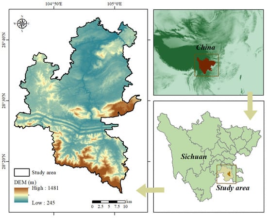
Figure 1.
The study area.
2.2. Data Sources and Preprocessing
This study utilized multi-source datasets including remote sensing data, land use data, and socioeconomic data to ensure a comprehensive analysis of social–ecological systems (Table 1). Land use data were acquired from the Resource and Environmental Sciences Data Center (https://www.resdc.cn/, accessed on 1 June 2024 2000, 2010, and 2023, 30 m resolution). Digital elevation model data were from the Shuttle Radar Topography Mission dataset. Vegetation remote sensing data (MOD13Q1 NDVI data; 2000–2022; 250 m resolution) were downloaded from NASA’s (United States National Aeronautics and Space Administration) Earth Science Data Systems (available online: https://www.earthdata.nasa.gov/eosdis, accessed on 1 June 2024; 2000–2022; 250 m resolution). Nighttime light imagery data were obtained from Harvard Dataverse (2000–2022; 500 m resolution; https://doi.org/10.7910/DVN/YGIVCD, accessed on 1 June 2024). Population density data were spatially prepared by considering the statistical population of villages and towns, land use types, and night light brightness (the influencing factor of population distribution). All datasets were uniformly processed and resampled to a consistent spatial resolution of 500 m in order to facilitate integrated analysis.

Table 1.
The description and sources of data used in this study.
2.3. Methods
To achieve our research objectives, we designed the following methodology flowchart (Figure 2), including three procedures—identifying TG, characterizing the evolution of the PLE, and examining the influence of PLE on TG. A complex system model was used to assess the interactions between human and natural systems. The “direction–speed–pattern” framework was used to measure multidimensional changes in the PLE of land use. Based on these results, this study quantified the driving force of TG based on PLE changes.

Figure 2.
Methodological flowchart of this study.
2.3.1. Human and Natural Systems
Social–ecological systems constitute interdependent subsystems that form integrated wholes across multiple spatiotemporal scales. Substantial empirical evidence demonstrates that biophysical and socioeconomic systems interact through complex, non-linear relationships that vary across spatial, temporal, and organizational dimensions, which is a fundamental characteristic of coupled social–ecological systems [67]. These interactions manifest most visibly through spatiotemporal changes in population distribution, vegetation patterns, and land use transitions, which collectively represent key indicators of human–environment dynamics [68,69]. Geographical landscapes and a single system can easily be identified through remote sensing means. Some studies indicate that vegetation cover is a key factor influencing the geographical distribution of uninhabited zones (areas with prominent natural ecological attributes) [41,67]. In the Sichuan Basin, low vegetation coverage means intensive human activities or high population density, while high vegetation coverage indicates a high natural component index. Human-induced land use changes have led to the loss and abandonment of areas with strong natural attributes, thereby enhancing the anthropogenic characteristics of the region [48]. Population and vegetation represent the most characteristic geographical elements of human and natural processes, respectively. At the county scale, we operationalize this framework by employing population dynamics as the primary socioeconomic system indicator and vegetation indices as the natural ecological proxy, with land use change processes serving as the critical interface [70]. The human-influenced intensity of land use exhibits an inverse relationship with natural system integrity, whereby as human modification intensifies, natural characteristics diminish proportionally [71]. This study leverages land use change data (2000–2022) from Changning County to enhance model robustness through longitudinal analysis, enabling the comprehensive characterization of TG evolution, land use spatiotemporal dynamics, and interactions between systems in mountainous regions. The extended temporal scope facilitates a deeper understanding of the development mechanisms of TG and the underlying mechanisms of human–natural coupling processes that shape transitional landscapes.
2.3.2. Complex System Model of Humans and Nature in Mountainous Counties
This study applies an improved coupling model integrated with trade-off analysis to quantitatively assess human–natural interactions, specifically measuring three key dimensions—coupling intensity, comprehensive level, and interaction directionality [48].
The coupling degree (PD) and coordination degree (CD) were calculated using the following formulae:
The natural ecosystem index (n) and socioeconomic system index (h) were derived from ecological and socioeconomic elements, respectively, with their relative contributions weighted by coefficients αₙ and αₕ. The trade-off (TO) relationship between these systems was quantified using the following formula:
These methodologies are illustrated in Figure 3, which provides a visual explanation of the three modeling approaches. To further integrate the capabilities of the three models, a complex system model was proposed by modifying the coupling model and the trade-off method. It was used as follows:
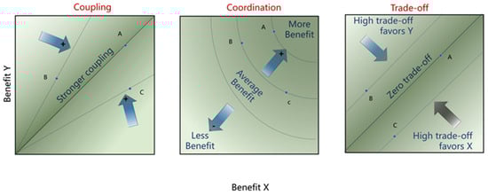
Figure 3.
Illustration and example of trade-offs and coordination between two benefits. The degree of trade-off between points A, B, and C is |A| > |B| = |C|.
The weighting coefficients αₕ and αₙ represent the relative contributions of the socioeconomic system index and natural ecosystem index, respectively. Based on the principle of equal importance between socioeconomic systems and natural ecosystems, this study employs an equal weighting approach, where αₕ = αₙ = 0.5. Here, the socioeconomic system index (h) quantifies socioeconomic dimensions, while the natural ecosystem index (n) assesses natural ecological dimensions.
2.3.3. Dynamic Degree
The degree of the spatial dynamics of PLE can reflect the speed of change, as well as changes in various types of land in a study area during a specific period of time. It is highly accurate in revealing the speed and degree of land type transformation and can effectively analyze the morphology of the study area in different periods from a macro-perspective. This study uses land use data to quantitatively analyze the changes in the quantity and area of the PLE, as well as the evolution of the structure in the study area. The calculation formula is as follows:
The coefficient K quantifies the dynamic utilization intensity of PLE during a specified time period, calculated as a function of initial (Aₘ) and final (Aₙ) spatial areas divided by the temporal interval (T). Higher absolute values of K correspond to more rapid and significant transformations in PLE configuration.
2.3.4. Transfer Matrices
We chose representative transfer matrices to evaluate the direction of the PLE and TG. The structural characteristics between different space utilization types can be quantitatively reflected using this matrix, thus revealing the conversion rate between different space utilization types.
Here, n denotes the number of various spaces, while Aij denotes the area of conversion from space type i to type j (i, j = 1, 2, 3, …, n).
3. Results
3.1. Evolution of TG
3.1.1. Identification of TG
The interaction degree of socioeconomic systems and natural ecosystems in Changning County is classified into five categories in this study using the natural break method (Table 2, Figure 4). The categories are as follows: dominated by SP (SP—socioeconomic process), strong SP–weak NP (NP—natural ecological process), semi-SP–semi-NP, strong NP–weak SP, and dominated by NP. Figure 4 shows the coverage of each type from 2000 to 2022. This result clearly shows that the spatial distribution of socioeconomic attributes in the study area exhibits a trend of “lower in the south and higher in the north”. It can be seen that the strong SP–weak NP areas are larger than those in other types and are mainly distributed in the north. The areas dominated by NP account for the smallest overall area. Strong NP–weak SP areas are mainly concentrated in the East and South Districts of Changning County, and the proportion of this type of area is lower than that of most other types, gradually decreasing over time. In 2022, the area was only 26.5 km2, accounting for merely 2.7% of the county’s total area. The strong SP–weak NP areas, semi-SP–semi-NP areas, and strong NP–weak SP areas, namely, the TG, are transition regions between the strong socioeconomic process areas and the strong natural ecological process areas.
Table 2.
Five types of transitions.

Figure 4.
The transitional geo-space (TG) in Changning County. Map (a–c) represent transitional geo-space in the years 2000, 2010, and 2022, respectively. NP = natural process, SP = social process.
3.1.2. Evolution of the TG Pattern
From 2000 to 2022, the transition types in the study area showed varying degrees of change (Figure 5). The changes in transition types became more pronounced from 2000 to 2010 (Figure 6). The area of semi-SP–semi-NP that converted into strong SP–weak NP was the largest (154.2 km2). Areas dominated by NP remained stable overall from 2000 to 2010, with only 3.2 km2 converted into strong SP–weak NP areas. Changes between transition types were less significant from 2010 to 2022 compared to the previous decade. The most notable transition was the conversion of strong NP–weak SP areas into semi-SP–semi-NP areas, covering only 24.5 km2. In both stages, semi-SP–semi-NP areas showed the most dynamic changes, whereby they first decreased to 203.9 km2 and then rebounded to 230.8 km2. The overall trend was downward, with semi-SP–semi-NP areas accounting for 24.3% of the total area by 2022.
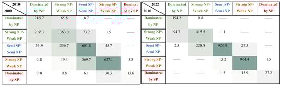
Figure 5.
Transfer matrix of the TG for Changning in the intervals 2000–2010 and 2010–2022 (km2).
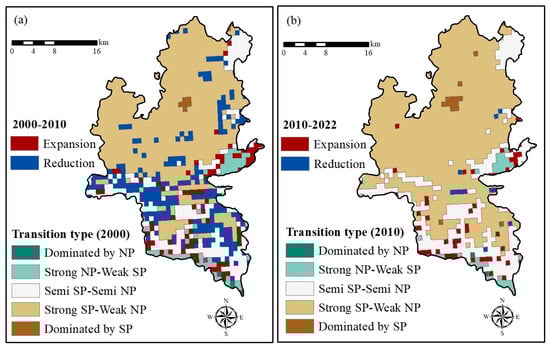
Figure 6.
TG evolution characteristics of Changning County, 2000–2022. Map (a,b) represent TG evolution between 2000–2010, and 2010–2022, respectively.
3.2. Changes in the PLE
3.2.1. Direction
In this study, we reclassified land use types from 2000 to 2022 (Figure 7) and calculated the areas of agricultural production space; industrial production space; rural living space; urban living space; ecological forest space; and grass, water, and other ecological spaces. Overall, the spatial change direction of the PLE is relatively stable. Figure 7a–c show that the most predominant PLE direction from 2010 to 2022 was the conversion of agricultural production space into other spaces. Production and living spaces are predominantly located in hilly areas, while ecological space is concentrated in mountainous areas. Human activities are mainly distributed in the north and central regions, and because of this, the transition stability of the ecological spaces is less affected by human interference. The agricultural production space has a greater distribution in the north and has the largest scale, accounting for over 70% of the total area, followed by forest–grass–water ecological spaces, which are primarily concentrated in the East and South Districts of Changning County. As shown in the data, the agricultural production space gradually decreased from 71.51% in 2000 to 70.76% in 2022. The ecological spaces of forest, grass, and water showed an overall trend of first increasing to 27.87% and then decreasing to 27.56%. Other spaces remained relatively stable over these two decades, with only a slight increase. The industrial production space, rural living space, and urban living space increased by 0.41%, 0.24%, and 0.32%, respectively (Figure 7d–f).
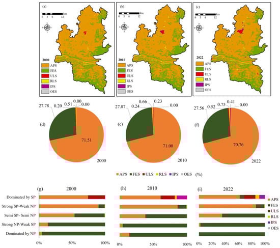
Figure 7.
Spatial evolution of the PLE in Changning County. Map (a–c) represent the spatial pattern of PLE in 2000, 2010, and 2022, respectively; Graph (d–f) represent the proportion of various PLE in 2000, 2010, and 2022, respectively; Graph (g–i) represent the proportion of various PLE in the TG in 2000, 2010, and 2022, respectively. APS = agricultural production space, FES = ecological spaces of forest, grass, and water, ULS = urban living space, RLS = rural living space, IPS = industrial production space, OES = other ecological spaces. NP = nature process, SP = social process.
From 2000 to 2022, urban living space, rural living space, and industrial production space were predominantly located in SP-dominated areas, with their spatial distributions evolving over time (Figure 7g–i). The analysis reveals three key trends. First, agricultural production space experienced a substantial decline of 12.40 percentage points over the 20-year period, while urban living space decreased by 8.5 percentage points. Second, both urban living space and forest–grass–water ecological spaces exhibited overall growth, whereas industrial production space showed an initial increase followed by a subsequent decrease. Third, agricultural production space constituted the primary land use type in strong SP–weak NP areas. Notably, forest–grass–water ecological space expanded by approximately 3 percentage points during the study period. Within transitional spaces, the proportion of forest–grass–water ecological space increased, while that of agricultural production space decreased. By 2022, the ecological spaces of forest, grass, and water had become the dominant land cover type in these transitional areas, accounting for over 60% of the total area.
A significant change was observed between different transition types in the study area from 2000 to 2022 (Figure 8a). In the strong NP–weak SP areas, the agricultural production space and the ecological spaces of forest, grass, and water were converted into each other. The transformation of agricultural production space into ecological spaces of forest, grass, and water occurred over the largest area (54.27 ha) from 2000 to 2010. Conversely, the transformation of ecological spaces of forest, grass, and water into agricultural production space was dominant (11.79 ha) from 2010 to 2022. From 2000 to 2010, the agricultural production space in semi-SP–semi-NP areas was mainly transformed into ecological spaces of forest, grass, and water, with a total of 151.28 ha of transformed land (Figure 8b). The ecological spaces of forest, grass, and water lost 152.46 ha to agricultural production land. From 2010 to 2022, the mutual conversion between agricultural production space and ecological spaces of forest, grass, and water was relatively high, both above 970 ha. Over the two decades, the transfer of PLE in strong SP–weak NP areas was transformed: the urban production space changed significantly from 49.95 ha in 2010 to 114.84 ha in 2022 (Figure 8c).
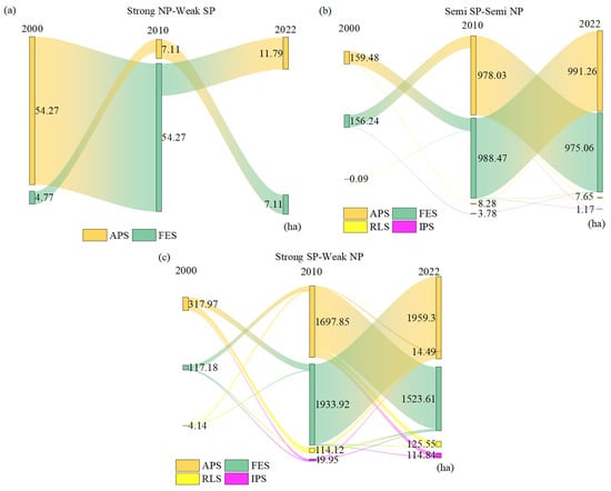
Figure 8.
Direction of spatial change in PLE in TG in Changning County. (a) Strong NP-Weak SP; (b) Semi SP-Semi NP; (c) Strong SP-Weak NP. APS = agricultural production space, FES = ecological spaces of forest, grass, and water, ULS = urban living space, RLS = rural living space, IPS = industrial production space, OES = other ecological spaces. NP = nature process; SP = social process.
3.2.2. Speed
We quantitatively evaluated changes in PLE using the degree of spatial dynamics (Figure 9a). High-value areas are concentrated in the north–central parts of the county, where human activities have significantly influenced the dynamic degree. Low-value zones, primarily located in the northwest and northern regions, are mainly characterized by agricultural activities. As shown in Figure 9b, areas dominated by SP have experienced the most substantial changes, showing a dynamic degree index of 1.13%. As these areas surround the city center, urban expansion and industrial development have accelerated urbanization. Consequently, urban living space and industrial production space have gradually replaced agricultural production space. In contrast, the least-changed region consists of areas dominated by SP (dynamic degree index: 0.00%), which are distant from urban centers and feature steep slopes and high elevations.
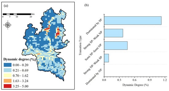
Figure 9.
The dynamic degree of PLE changes in Changning County. (a) spatial pattern of dynamic degree; (b) the dynamic degree of various transition type. Strong NP = nature process; SP = social process.
3.2.3. Pattern
Annual changes in landscape indices (LPI, SHDI, FRAC_AM, and CONTAG) demonstrate how PLE transformations influence landscape patterns (Figure 10). High LPI and CONTAG values predominantly occur in the northern region, reflecting dynamic environmental and socioeconomic interactions. Peak SHDI and FRAC_AM values are concentrated in southern areas, where limited human activity maintains lower landscape complexity. During the period from 2000 to 2022, the landscape in the areas dominated by SP, as well as the strong SP–weak NP areas, became more complex in shape, with an increase in fragmentation, as well as an increase in aggregation and connectivity (Table 3). These changes suggest significant anthropogenic disturbance effects. At the landscape level, LPI shows increasing trends (increases by 3.754), while SHDI, FRAC_AM, and CONTAG decrease by 0.085, 0.009, and 17.089, respectively, indicating that the landscape pattern in the areas dominated by NP, as well as strong NP–weak SP areas and areas dominated by NP, developed more consistently over time.

Figure 10.
Spatial distribution of landscape patterns for production–living–ecological spaces in Changning County. Maps (a–l) represent the various landscape patterns in 2000, 2010, and 2022, respectively.
Table 3.
Landscape patterns in the PLE of various transitional types in Changning County from 2000 to 2020.
3.3. Impacts of Spatial Variations in the PLE on TG
Correlation analysis revealed significant associations between land use elements and the TG (Figure 11). We examined the influence of the PLE on the TG through three dimensions. Among various PLE directions, a significant negative correlation was observed between the TG and the change direction of the PLE between 2000 and 2010, especially in relation to the conversion of agricultural production spaces into forest–grass–water ecological spaces (R2 = −0.295; p < 0.01). Strong negative impacts occurred when ecological space was converted into agricultural production space, whether in the first decade (R2 = −0.28; p < 0.01) or the second decade (R2 = −0.24; p < 0.01). The change speed of the PLE exhibited obvious negative correlations between 2000 and 2010 (R2 = −0.247; p < 0.01) and between 2010 and 2022 (R2 = −0.135; p < 0.05). This implies that the expansion of TG is prevented by rapid changes in the PLE. In the pattern dimension, LPI showed a significant positive correlation with the TG from 2000 to 2022, while SHDI showed a negative correlation. Although FRAC_AM had a stronger impact on the TG, and CONTAG had a weaker impact on the TG, both of them had contrasting effects on the TG in the two time periods.

Figure 11.
Influence of direction–velocity–pattern dimensions on TG. APS = agricultural production space, FES = ecological spaces of forest, grass, and water, ULS = urban living space, and RLS = rural living space.
4. Discussion
4.1. Evolution of the TG
Our study’s findings both align with and differ from previous TG research, offering new insights into TG dynamics in mountainous regions. While our results corroborated some general trends observed in the existing literature, they also revealed unique patterns specific to Changning County’s mountainous context. An analysis of transition types in Changning County over the past two decades revealed a gradual increase in anthropogenic influences. PLE changes were primarily driven by multiple factors, including urbanization processes, land use policies, technological advancements, and the livelihood transformations of farming households. The changes in the PLE led to changes in landscapes and patterns of land use, which, in turn, determined changes in the TG. The areas dominated by SP and strong SP–weak NP areas in Changning County have been constantly increasing, while the core area of TG, which is a semi-SP–semi-NP area, has been transitioning into an area dominated by NP (Figure 4 and Figure 8). Under China’s rural revitalization strategy, the rural territorial system is undergoing significant transition and reconstruction. This process encompasses both the socioeconomic restructuring and functional enhancement of territorial spaces [72]. Accelerated urbanization has triggered growing demand for construction and residential lands, while simultaneously reducing farmland and forest cover in peri-urban areas. These changes have diminished land capacities for food production and biodiversity conservation but enhanced capabilities for human settlement support. Both natural and anthropogenic disturbances may significantly alter ecotones between adjacent ecosystems, which are referred to as TGs in our study [73,74,75]. Boundary dynamics in transitional zones (ecotones) exhibit significant seasonal and interannual fluctuations [76]. For example, ecotones demonstrate particular sensitivity to environmental variations, and their dynamic spatial shifts serve as reliable indicators of environmental change [77]. However, the changes in TG in the social ecological system are mainly reflected in interannual variations. If rainfall decreases in a given year, farmers are expected to compensate for the decrease in production by expanding the area they use. If rainfall is above average, farmers use less land to produce the same amount of food [78,79]. Such changes directly affect the growth and distribution of vegetation, and fluctuations in precipitation can also stimulate interest in newly cleared land. As a result, production patterns between crop growth and animal husbandry have changed in response to precipitation variations in the farming–pastoral ecotone of China [80]. This also affects the distribution of grasslands and cultivated land in Changning County, leading to changes in the area dominated by SP and areas of strong SP–weak NP in the TG. A study on the Sudanese–Sahelian countries in mountainous areas shows that human changes have driven the expansion of arable land and increased the demand for food crop consumption, while inter-annual variations in rainfall have altered land productivity in the Sahel [73]. Land use is primarily driven by three interrelated factors—population growth, biophysical environment degradation, and escalating demand for cash crop cultivation [81,82]. Although technological change represents another significant driver, it should not be considered the sole determinant of agricultural transformation and TG changes [83].
4.2. Drivers of TG
As a significant agricultural county in southern Sichuan Province [84], Changning County exhibits a distinct spatial pattern dominated by agricultural production areas, complemented by forest–grass–water ecological spaces, with the relatively flat northern terrain being particularly favorable to both agricultural activities and human settlements. This spatial configuration stems from favorable natural geographic conditions, enhanced infrastructure development, and economic restructuring. Over the past two decades, substantial improvements in transportation networks and medical facilities have significantly increased the region’s attractiveness, promoting settlement expansion and population concentration. To better understand the coupled human–natural evolution of TG in Changning County, we employed four landscape pattern indices (LPI, SHDI, FRAC_AM, and CONTAG) to characterize different stages of geospatial transformation. From a landscape ecology perspective, varying land use combinations create distinct landscape structures, where landscape development essentially represents the conversion of natural landscapes into anthropogenic ones [5,85]. These indices effectively capture the spatial transition patterns of PLE across the study area.
As shown in Figure 11, there is a significant negative correlation between the direction of change and TG in the PLE in Changning County. In terms of speed, the speed of PLE changes in Changning County has a significant negative effect on TG expansion. The pattern of change in the PLE shows that all indices have a significant effect on the TG in Changning County, except for CONTAG. Accelerated urban expansion and rural settlement encroachment into natural areas have intensified soil sealing and degradation processes [86]. These patterns must be considered within China’s rural revitalization strategy, which emphasizes balanced development across five dimensions—thriving industries, eco-friendly habitats, cultural prosperity, effective governance, and prosperity [10]. This policy framework drives a fundamental transition in land use paradigms—from production-dominated approaches to integrated ecological–production–living systems. As spatial interactions between landscape features inevitably create functional trade-offs [87], sustainable development planning should adopt place-based strategies that respect local resource endowments and promote functional synergies to achieve high-quality socioeconomic development.
4.3. Shortcomings and Prospects
Strong SP-weak NP areas are significantly affected by human activities, with frequent disturbances from town construction and rural agricultural production activities. In the future, efforts should be made to adjust and optimize the structure and spatial layout of agricultural production, and promote the comprehensive enhancement of agro-ecological capacity. In the semi-SP–semi-NP areas, the area of rural living space is centrally distributed. The relationship between urban and rural areas here is more complex, facing the problem of a widening gap between urban and rural areas. It is necessary to clarify the complex function of the land space and promote the coordinated development of different function types. The utilization of land in the agro-ecological area of strong NP–weak SP is dominated by agricultural production; rural living; and forest, grass, and water ecological spaces. The weak interference of human activities is the main feature. Therefore, land improvement projects should be implemented in the region to enhance the economic benefits of agricultural production space, improve the rural living environment, and achieve geospatial optimization.
As a typical TG in mountainous areas, Changning County plays a crucial role in regional sustainable development, food security, land resource allocation, and ecological protection. Based on multi-source and multi-scale data, such as land use data, socioeconomic data, and remote sensing data, this study quantifies the land use function of TG at the raster scale and reveals the influence of the PLE on TG. However, the evolution of the spatial and temporal pattern of the TG in Changning County from 2000 to 2022 was also affected by many other uncontrollable natural factors and multi-level human social and economic factors. What is more, this kind of research needs to involve a wide range of scientific fields. There should be a much more complicated analysis of the evolution of TG in Changning County. Therefore, more factors should be considered in future research. Additionally, expanding the time range of the study and reducing the time intervals can capture longer-term, more detailed, and comprehensive trends in TG.
5. Conclusions
TG has inimitable human–environment relationship characteristics in coupled socioecological systems, where landscape management and planning are closely linked to the well-being of people and nature. Responding to China’s policy emphasis on optimizing land use structures for ecological–production–living coordination, we employed multi-source geospatial data and coupled human–natural system modeling to analyze TG evolution. By analyzing the spatial and temporal evolution of TG changes in terms of the spatial distribution pattern of PLE, it was found that the speed of change and direction of transfer are more scientific and effective research metrics. The results are as follows.
(1) When choosing indicative elements, we characterized dynamic human and natural systems in terms of dynamic population and vegetation, respectively. Spatial and temporal changes in land use can be seen as elements of an integrated characterization of the spatial and temporal dynamics of human–natural interactions. Transition types can be categorized into five categories by measuring the strength and direction of interactions between human and natural systems through complex system models.
(2) The overall terrain of Changning County is low, with many hills and low mountains. Human activities are not easily restricted by topography, and most of the study area is strong SP–weak NP (79.3% of the area in 2022). With an increase in human activities and the expansion of construction land, the TG begins to approach the area dominated by NP.
(3) A large amount of cultivated land (area over 660 km2) is distributed in Changning County, and the study area has an increasing topography from south to north. Human activities and agricultural production are mainly distributed in the central and northern parts. The south has high forest cover and only a few agricultural patches, with less intensive land use but with high ecosystem service provision and ecological importance, which shapes land cover and thus determines the landscape index.
The direction of transfer, speed of change, and distribution pattern of the PLE in the study area have different driving mechanisms for TG changes. From 2000 to 2022, the fastest changes in the PLE in Changning County were mainly distributed in the northern part of the county, followed by the area along the river. Strong negative impacts occurred when ecological space was converted into agricultural production space, whether in the first decade (R2 = −0.28, p < 0.01) or the second decade (R2 = −0.24, p < 0.01).
Author Contributions
Conceptualization, X.L., X.Z., S.Z. and H.Z.; Funding acquisition, H.Z.; Investigation, Y.X., X.Z. and S.Z.; Methodology, X.L., X.Z. and S.Z.; Software, Y.X.; Supervision, X.Z. and H.Z.; Validation, X.Z. and H.Z.; Writing—original draft, Y.X. and X.L.; Writing—review and editing, Y.X., X.L. and H.Z. All authors have read and agreed to the published version of the manuscript.
Funding
This research was funded by National Natural Science Foundation of China (No. 42401354) and Sichuan Philosophy and Social Science Foundation project (No. SCJJ23ND427).
Data Availability Statement
The data presented in this study are available upon request from the corresponding author. The data are not publicly available due to privacy.
Conflicts of Interest
The authors declare no conflicts of interest.
References
- He, C.; Liu, Z.; Tian, J.; Ma, Q. Urban Expansion Dynamics and Natural Habitat Loss in China: A Multiscale Landscape Perspective. Glob. Change Biol. 2014, 20, 2886–2902. [Google Scholar] [CrossRef]
- He, C.; Zhao, Y.; Tian, J.; Shi, P. Modeling the Urban Landscape Dynamics in a Megalopolitan Cluster Area by Incorporating a Gravitational Field Model with Cellular Automata. Landsc. Urban Plann. 2013, 113, 78–89. [Google Scholar] [CrossRef]
- He, C.; Zhang, D.; Huang, Q.; Zhao, Y. Assessing the Potential Impacts of Urban Expansion on Regional Carbon Storage by Linking the LUSD-Urban and InVEST Models. Environ. Modell. Softw. 2016, 75, 44–58. [Google Scholar] [CrossRef]
- Zhou, L.; Wei, L.; López-Carr, D.; Dang, X.; Yuan, B.; Yuan, Z. Identification of irregular extension features and fragmented spatial governance within urban fringe areas. Appl. Geogr. 2024, 162, 103172. [Google Scholar] [CrossRef]
- Peng, J.; Wang, Y.; Zhang, Y.; Wu, J.; Li, W.; Li, Y. Evaluating the Effectiveness of Landscape Metrics in Quantifying Spatial Patterns. Ecol. Indic. 2010, 10, 217–223. [Google Scholar] [CrossRef]
- Duan, Y.; Wang, H.; Huang, A.; Xu, Y.; Lu, L.; Ji, Z. Identification and Spatial-Temporal Evolution of Rural “Production-Living-Ecological” Space from the Perspective of Villagers’ Behavior—A Case Study of Ertai Town, Zhangjiakou City. Land Use Policy 2021, 106, 105457. [Google Scholar] [CrossRef]
- Hahs, A.K.; McDonnell, M.J. Selecting Independent Measures to Quantify Melbourne’s Urban–Rural Gradient. Landsc. Urban Plann. 2006, 78, 435–448. [Google Scholar] [CrossRef]
- Shin, Y.A.; Lacasse, K.; Gross, L.J.; Beckage, B. How Coupled Is Coupled Human-Natural Systems Research? Ecol. Soc. 2022, 27, art4. [Google Scholar] [CrossRef]
- Peng, L.; Deng, W.; Zhang, H.; Sun, J.; Xiong, J. Focus on Economy or Ecology? A Three-dimensional Trade-off Based on Ecological Carrying Capacity in Southwest China. Nat. Resour. Model. 2019, 32, e12201. [Google Scholar] [CrossRef]
- Zou, L.; Liu, Y.; Wang, J.; Yang, Y. An Analysis of Land Use Conflict Potentials Based on Ecological-Production-Living Function in the Southeast Coastal Area of China. Ecol. Indic. 2021, 122, 107297. [Google Scholar] [CrossRef]
- Fagioli, F.F.; Rocchi, L.; Paolotti, L.; Słowiński, R.; Boggia, A. From the Farm to the Agri-Food System: A Multiple Criteria Framework to Evaluate Extended Multi-Functional Value. Ecol. Indic. 2017, 79, 91–102. [Google Scholar] [CrossRef]
- Paracchini, M.L.; Pacini, C.; Jones, M.L.M.; Pérez-Soba, M. An Aggregation Framework to Link Indicators Associated with Multifunctional Land Use to the Stakeholder Evaluation of Policy Options. Ecol. Indic. 2011, 11, 71–80. [Google Scholar] [CrossRef]
- Huang, J.; Lin, H.; Qi, X. A literature review on optimization of spatial development pattern based on ecological-production-living space. Prog. Geogr. 2017, 36, 378–391. [Google Scholar]
- Huang, Q.; Song, W.; Song, C. Consolidating the Layout of Rural Settlements Using System Dynamics and the Multi-Agent System. J. Clean. Prod. 2020, 274, 123150. [Google Scholar] [CrossRef]
- Liu, C.; Xu, Y.; Huang, A.; Liu, Y.; Wang, H.; Lu, L.; Sun, P.; Zheng, W. Spatial Identification of Land Use Multifunctionality at Grid Scale in Farming-Pastoral Area: A Case Study of Zhangjiakou City, China. Habitat Int. 2018, 76, 48–61. [Google Scholar] [CrossRef]
- Wang, S.; Kong, W.; Ren, L.; Zhi, D.; Dai, B. Research on misuses and modification of coupling coordination degree model in China. J. Nat. Resour. 2021, 36, 793–810. [Google Scholar] [CrossRef]
- Zhou, H.; Wang, C.; Bai, Y.; Ning, X.; Zang, S. Spatial and Temporal Distribution of Rural Settlements and Influencing Mechanisms in Inner Mongolia, China. PLoS ONE 2022, 17, e0277558. [Google Scholar] [CrossRef]
- Zhou, H.; Ning, X.; Li, W. Spatial distribution variation of rural settlements in Damao Banner of Baotou City and its impact factors. Trans. Chin. Soc. Agric. Eng. 2019, 35, 276–286. [Google Scholar]
- Li, Y.; Li, Y.; Zhou, Y.; Shi, Y.; Zhu, X. Investigation of a Coupling Model of Coordination between Urbanization and the Environment. J. Environ. Manag. 2012, 98, 127–133. [Google Scholar] [CrossRef]
- Hussain, J.; Zhou, K.; Guo, S.; Khan, A. Investment Risk and Natural Resource Potential in “Belt & Road Initiative” Countries: A Multi-Criteria Decision-Making Approach. Sci. Total Environ. 2020, 723, 137981. [Google Scholar] [CrossRef]
- Zhou, H.; Na, X.; Li, L.; Ning, X.; Bai, Y.; Wu, X.; Zang, S. Suitability Evaluation of the Rural Settlements in a Farming-Pastoral Ecotone Area Based on Machine Learning Maximum Entropy. Ecol. Indic. 2023, 154, 110794. [Google Scholar] [CrossRef]
- Shen, W.; Zhou, T.; Chang, H.; Qiu, X.; Liu, Y.; Sun, H.; Zhai, X.; Yang, H.; Liu, G.; Yang, W. Responses of Grazing Households to Different Levels of Payments for Ecosystem Services. Ecosyst. Health Sustain. 2022, 8, 2052762. [Google Scholar] [CrossRef]
- Yi, J.; Li, H.; Wang, D.; Huo, Z. Spatial-temporal change and coupling coordination measurement of rural territorial multi-functions in Jilin Province. China Land Sci. 2021, 35, 63–73. [Google Scholar]
- Mander, Ü.; Helming, K.; Wiggering, H. Multifunctional Land Use: Meeting Future Demands for Landscape Goods and Services. In Multifunctional Land Use; Springer: Berlin/Heidelberg, Germany, 2007; pp. 1–13. ISBN 978-3-540-36763-5. [Google Scholar]
- Vizzari, M.; Sigura, M. Landscape Sequences along the Urban–Rural–Natural Gradient: A Novel Geospatial Approach for Identification and Analysis. Landsc. Urban Plann. 2015, 140, 42–55. [Google Scholar] [CrossRef]
- Zou, L.; Liu, Y.; Yang, J.; Yang, S.; Wang, Y.; Zhi, C.; Hu, X. Quantitative Identification and Spatial Analysis of Land Use Ecological-Production-Living Functions in Rural Areas on China’s Southeast Coast. Habitat Int. 2020, 100, 102182. [Google Scholar] [CrossRef]
- Yang, Y.; Bao, W.; Liu, Y. Coupling Coordination Analysis of Rural Production-Living-Ecological Space in the Beijing-Tianjin-Hebei Region. Ecol. Indic. 2020, 117, 106512. [Google Scholar] [CrossRef]
- Bennich, T.; Weitz, N.; Carlsen, H. Deciphering the Scientific Literature on SDG Interactions: A Review and Reading Guide. Sci. Total Environ. 2020, 728, 138405. [Google Scholar] [CrossRef]
- Fu, J.; Bu, Z.; Jiang, D.; Lin, G.; Li, X. Sustainable Land Use Diagnosis Based on the Perspective of Production–Living–Ecological Spaces in China. Land Use Policy 2022, 122, 106386. [Google Scholar] [CrossRef]
- Akuraju, V.; Pradhan, P.; Haase, D.; Kropp, J.P.; Rybski, D. Relating SDG11 Indicators and Urban Scaling—An Exploratory Study. Sustain. Cities Soc. 2020, 52, 101853. [Google Scholar] [CrossRef]
- Liu, J.; Wang, J.; Zhai, T.; Li, Z.; Huang, L.; Yuan, S. Gradient Characteristics of China’s Land Use Patterns and Identification of the East-West Natural-Socio-Economic Transitional Zone for National Spatial Planning. Land Use Policy 2021, 109, 105671. [Google Scholar] [CrossRef]
- Chen, S.; Xu, G.; Lu, Z.; Ma, M.; Li, H.; Zhu, Y. Spatiotemporal variations of fractional vegetation cover and its response to climate change and urbanization in China. Arid. Land Geogr. 2023, 46, 742–752. [Google Scholar]
- Xu, Z.; Zhang, Z.; Li, C. Exploring Urban Green Spaces in China: Spatial Patterns, Driving Factors and Policy Implications. Land Use Policy 2019, 89, 104249. [Google Scholar] [CrossRef]
- Li, Y.; Sun, J.; Wang, M.; Guo, J.; Wei, X.; Shukla, M.K.; Qi, Y. Spatiotemporal Variation of Fractional Vegetation Cover and Its Response to Climate Change and Topography Characteristics in Shaanxi Province, China. Appl. Sci. 2023, 13, 11532. [Google Scholar] [CrossRef]
- Xu, Y.; Yu, L.; Peng, D.; Zhao, J.; Cheng, Y.; Liu, X.; Li, W.; Meng, R.; Xu, X.; Gong, P. Annual 30-m Land Use/Land Cover Maps of China for 1980–2015 from the Integration of AVHRR, MODIS and Landsat Data Using the BFAST Algorithm. Sci. China Earth Sci. 2020, 63, 1390–1407. [Google Scholar] [CrossRef]
- Naiman, R.; Décamps, H. The Ecology and Management of Aquatic-Terrestrial Ecotones; CRC Press: Boca Raton, FL, USA, 1990. [Google Scholar]
- Cadenasso, M.L.; Traynor, M.M.; Pickett, S.T. Functional Location of Forest Edges: Gradients of Multiple Physical Factors. Can. J. For. Res. 1997, 27, 774–782. [Google Scholar] [CrossRef]
- Laurance, W.F.; Didham, R.K.; Power, M.E. Ecological Boundaries: A Search for Synthesis. Trends Ecol. Evol. 2001, 16, 70–71. [Google Scholar] [CrossRef]
- Kutuzov, A. The Use of Modern and Archive Remote Sensing Data for GIS Monitoring of Riparian Ecosystems. Ecosyst. Transform. 2018, 1, 1–5. [Google Scholar] [CrossRef]
- Chen, Q. “Hu Population Line” and the Transitional Border between Agriculture and Pasture: A Discussion from a New Perspective. Pratacultural. Sci. 2018, 35, 669–676. [Google Scholar]
- Wei, C.; Aijia, L.; Yungang, H.; Lihe, L.; Haimeng, Z.; Xuerong, H.; Bin, Y. Exploring the Long-Term Vegetation Dynamics of Different Ecological Zones in the Farming-Pastoral Ecotone in Northern China. Environ. Sci. Pollut. Res. 2021, 28, 27914–27932. [Google Scholar]
- Sun, F.; Wang, Y.; Chen, Y.; Li, Y.; Kayumba, P.M. Historic and Simulated Desert-Oasis Ecotone Changes in the Arid Tarim River Basin, China. Remote Sens. 2021, 13, 647. [Google Scholar] [CrossRef]
- Yu, K.; Feng, Y.; Zheng, J.; Li, X.; Li, Z. Land use changes and their ecological effects in urban-rural ecotone. Trans. Chin. Soc. Agric. Eng. 2009, 25, 213–218. [Google Scholar]
- Yuxin, F.; University, N.N. Northwestern Farming-Pastoral Zones in the Perspective of Historical Geography. J. Arid Land Resour. Environ. 2019, 33, 83–89. [Google Scholar]
- Zhang, H.; Liu, F.; Zhang, J. Using composite system index to identify China’s ecological and socio-economic transition zone. Front. Plant Sci. 2022, 13, 1057271. [Google Scholar] [CrossRef]
- Yang, Y.; Liu, Y.; Li, Y.; Du, G. Quantifying Spatio-Temporal Patterns of Urban Expansion in Beijing during 1985–2013 with Rural-Urban Development Transformation. Land Use Policy 2018, 74, 220–230. [Google Scholar] [CrossRef]
- Changnon, S.A.; Kunkel, K.E.; Winstanley, D. Climate Factors That Caused the Unique Tall Grass Prairie in the Central United States. Phys. Geogr. 2002, 23, 259–280. [Google Scholar] [CrossRef]
- Deng, W.; Zhang, H.; Zhang, S.; Wang, Z.; Hu, M.; Peng, L. How to Identify Transitional Geospace in Mountainous Areas?: An Approach Using a Transitional Index from the Perspective of Coupled Human and Natural Systems. J. Geogr. Sci. 2023, 33, 1205–1225. [Google Scholar] [CrossRef]
- Peng, J.; Zhao, S.; Liu, Y.; Tian, L. Identifying the Urban-Rural Fringe Using Wavelet Transform and Kernel Density Estimation: A Case Study in Beijing City, China. Environ. Model. Softw. 2016, 83, 286–302. [Google Scholar] [CrossRef]
- Foody, G.M.; Boyd, D.S. Detection of Partial Land Cover Change Associated with the Migration of Inter-Class Transitional Zones. Int. J. Remote Sens. 1999, 20, 2723–2740. [Google Scholar] [CrossRef]
- Camarero, J.J.; Gutiérrez, E.; Fortin, M. Spatial Patterns of Plant Richness across Treeline Ecotones in the Pyrenees Reveal Different Locations for Richness and Tree Cover Boundaries. Glob. Ecol. Biogeogr. 2006, 15, 182–191. [Google Scholar] [CrossRef]
- Pitas, I. Digital Image Processing Algorithms and Applications. IEEE Signal Process. Mag. 2001, 18, 58. [Google Scholar] [CrossRef]
- Wang, H.; Zhang, X.; Kang, T. Urban Fringe Division and Feature Analysis Based on the Multi-Criterion Judgment. J. Nat. Resour. 2011, 26, 703–714. [Google Scholar]
- Zhang, M.; Meng, X.; Wang, L.; Xu, T. Transit Development Shaping Urbanization: Evidence from the Housing Market in Beijing. Habitat Int. 2014, 44, 545–554. [Google Scholar] [CrossRef]
- Imhoff, M.L.; Zhang, P.; Wolfe, R.E.; Bounoua, L. Remote Sensing of the Urban Heat Island Effect across Biomes in the Continental USA. Remote Sens. Environ. 2010, 114, 504–513. [Google Scholar] [CrossRef]
- Zhang, C.; Tian, H.; Chen, G.; Chappelka, A.; Xu, X.; Ren, W.; Hui, D.; Liu, M.; Lu, C.; Pan, S.; et al. Impacts of Urbanization on Carbon Balance in Terrestrial Ecosystems of the Southern United States. Environ. Pollut. 2012, 164, 89–101. [Google Scholar] [CrossRef]
- Zhang, C.; Tian, H.; Pan, S.; Liu, M.; Lockaby, G.; Schilling, E.B.; Stanturf, J. Effects of Forest Regrowth and Urbanization on Ecosystem Carbon Storage in a Rural–Urban Gradient in the Southeastern United States. Ecosystems 2008, 11, 1211–1222. [Google Scholar] [CrossRef]
- Sun, X.; Zhang, B.; Ye, S.; Grigoryan, S.; Zhang, Y.; Hu, Y. Spatial pattern and coordination relationship of production–living–ecological space function and residents’ behavior flow in rural–urban fringe areas. Land 2024, 13, 446. [Google Scholar] [CrossRef]
- Doum, R.; Zhangm, S.; Liu, X. Spatial and temporal diversity patterns and influencing factors in “production system-life systemecosystem” coupled coordination in resource-based cities in China. J. Beijing Norm. Univ. Sci. 2021, 57, 9. [Google Scholar] [CrossRef]
- Lemieux, L.T. Regression Discontinuity Designs in Economics. J. Econ. Lit. 2010, 48, 281–355. [Google Scholar] [CrossRef]
- Yang, L.; Li, Y.; Shan, B.; Shi, L. Spatial variation of soil organic carbon in bamboo forests: A case study in Changning County, Sichuan Province. Chin. J. Ecol. 2023, 42, 854–861. [Google Scholar] [CrossRef]
- Wang, Z.; Deng, W.; Zhang, S.; Zhang, H. Analysis of Multifunctionality and Transitional Geospatial Correlation of Mountainous Land—A Case Study of Changning County. Geogr. Sci. 2022, 42, 1091–1101. [Google Scholar] [CrossRef]
- Kelin, C. 40 years of China’s turning counties into suburban districts: Review and reflection. Local Gov. Res. 2019, 2–19, 78. [Google Scholar]
- Peng Xi; Chen Zhongchang Impact evaluation on China’s western development policy. China Popul. Resour. Environ. 2016, 26, 136–144.
- Chen, M.; Li, Y.; Gong, Y.; Lu, D.; Zhang, H. Exploring the spatial differentiation of urbanization on two sides of the Hu Huanyong Line–based on nighttime light data and cellular automata. Acta Geogr. Sin. 2016, 71, 179–193. [Google Scholar] [CrossRef]
- Wang, J.; Chen, Y.; Shao, X.; Zhang, Y.; Cao, Y. Land-Use Changes and Policy Dimension Driving Forces in China: Present, Trend and Future. Land Use Policy 2012, 29, 737–749. [Google Scholar] [CrossRef]
- Jin, F.; Wang, C.; Li, X.; Wang, J. China’s regional transport dominance: Density, proximity, and accessibility. J. Geogr. Sci. 2010, 20, 295–309. [Google Scholar] [CrossRef]
- Ge, D.; Zhou, G.; Qiao, W.; Yang, M. Land Use Transition and Rural Spatial Governance: Mechanism, Framework and Perspectives. J. Geogr. Sci. 2020, 30, 1325–1340. [Google Scholar] [CrossRef]
- Wu, S.; Liang, Z.; Li, S. Relationships between Urban Development Level and Urban Vegetation States: A Global Perspective. Urban For. Urban Green. 2019, 38, 215–222. [Google Scholar] [CrossRef]
- Li, S.; Li, X. Economic characteristics and the mechanism of farmland marginalization in mountainous areas of China. Acta Geogr. Sin. 2018, 73, 803–817. [Google Scholar]
- Zhang, S.; Deng, W.; Hu, M.; Zhang, H.; Wang, Z.; Peng, L. Identification and Differentiation Analysis of Human-Nature Interaction in Transitional Geospatial Areas of Mountainous Regions. Acta Geogr. Sin. 2022, 77, 1225–1243. [Google Scholar]
- Li, H.; Hu, X.; Zhang, X.; Li, Z.; Yuan, Y. Analysis of Rural Space. Prog. Geogr. 2018, 37, 591–600. [Google Scholar]
- Stéphenne, N.; Lambin, E.F. A Dynamic Simulation Model of Land-Use Changes in Sudano-Sahelian Countries of Africa (SALU). Agric. Ecosyst. Environ. 2001, 85, 145–161. [Google Scholar] [CrossRef]
- Pogue, D.W.; Schnell, G.D. Effects of Agriculture on Habitat Complexity in a Prairie-Forest Ecotone in the Southern Great Plains of North America. Agric. Ecosyst. Environ. 2001, 87, 287–298. [Google Scholar] [CrossRef]
- Lambin, E.F.; Turner, B.L.; Geist, H.J.; Agbola, S.B.; Angelsen, A.; Bruce, J.W.; Coomes, O.T.; Dirzo, R.; Fischer, G.; Folke, C.; et al. The Causes of Land-Use and Land-Cover Change: Moving beyond the Myths. Glob. Environ. Change 2001, 11, 261–269. [Google Scholar] [CrossRef]
- Fortin, M.-J.; Olson, R.J.; Ferson, S. Issues Related to the Detection of Boundaries. Landsc. Ecol. 2000, 15, 453–466. [Google Scholar] [CrossRef]
- Crumley, C.L. Analyzing Historic Ecotonal Shifts. Ecol. Appl. 1993, 3, 377–384. [Google Scholar] [CrossRef]
- Wezel, A.; Böcker, R. Mulching with Branches of an Indigenous Shrub (Guiera Senegalensis) and Yield of Millet in Semi-Arid Niger. Soil Tillage Res. 1999, 50, 341–344. [Google Scholar] [CrossRef]
- Wezel, A.; Rath, T. Resource Conservation Strategies in Agro-Ecosystems of Semi-Arid West Africa. J. Arid. Environ. 2002, 51, 383–400. [Google Scholar] [CrossRef]
- Liu, J.; Gao, J.; Lv, S.-H.; Han, Y.; Nie, Y. Shifting Farming–Pastoral Ecotone in China under Climate and Land Use Changes. J. Arid. Environ. 2011, 75, 298–308. [Google Scholar] [CrossRef]
- Reenberg, A. A Hierarchical Approach to Land Use and Sustainable Agriculture in the Sahel. Q. J. Int. Agric. 1996, 35, 63–77. [Google Scholar]
- Reenberg, A.; Markussen, B. Sahel, Population, Integrated Rural Development Projects, and Research Components in Development Projects; Aarhus University Press: Aarhus, Denmark, 1994. [Google Scholar]
- Walker, T.S. Smallholders, Householders: Farm Families and the Ecology of Intensive, Sustainable Agriculture. Agric. Syst. 1997, 53, 317–319. [Google Scholar] [CrossRef]
- Luo, Q.; Li, W.; Zhang, J. Construction and analysis of evaluation index system of rural vitalization’s comprehensive development level: A case study of Changning County, Sichuan Province. Food Sci. Technol. Econ. 2023, 48, 32–35. [Google Scholar] [CrossRef]
- Peng, J.; Ma, J.; Yuan, Y. Research Progress and Prospect on the Identification of Urban Fringe. Prog. Geogr. 2014, 33, 1068–1077. [Google Scholar] [CrossRef]
- Amato, F.; Maimone, B.; Martellozzo, F.; Nolè, G.; Murgante, B. The Effects of Urban Policies on the Development of Urban Areas. Sustainability 2016, 8, 297. [Google Scholar] [CrossRef]
- Liberati, M.R.; Rittenhouse, C.D.; Vokoun, J.C. Addressing Ecological, Economic, and Social Tradeoffs of Refuge Expansion in Constrained Landscapes. Landsc. Ecol. 2019, 34, 627–647. [Google Scholar] [CrossRef]
Disclaimer/Publisher’s Note: The statements, opinions and data contained in all publications are solely those of the individual author(s) and contributor(s) and not of MDPI and/or the editor(s). MDPI and/or the editor(s) disclaim responsibility for any injury to people or property resulting from any ideas, methods, instructions or products referred to in the content. |
© 2025 by the authors. Licensee MDPI, Basel, Switzerland. This article is an open access article distributed under the terms and conditions of the Creative Commons Attribution (CC BY) license (https://creativecommons.org/licenses/by/4.0/).