Abstract
The construction of high-speed railway (HSR) station areas serves as a crucial catalyst for urban spatial evolution. However, the absence of targeted urban management theories has led to widespread spatial resource waste and post-construction abandonment phenomena in these areas. Existing research predominantly focuses on development strategies for individual construction elements of HSR stations yet lacks comprehensive strategy formulation through coordinated multi-level elements from a sustainable perspective. This study establishes a national database comprising 1018 HSR station area samples across China in 2020, integrating built environment characteristics, HSR network topology, ecological considerations, and socioeconomic indicators. Guided by the land equilibrium utilization theory, we employ the random forest Boruta algorithm to identify critical features, using land supply capacity and development intensity as target variables. Subsequently, K-means++ clustering analysis based on these key variables categorizes the samples into nine distinct clusters. Through normal distribution tests, we establish reference ranges for cluster-specific indicators and propose tailored development strategies across multiple dimensions. This research develops a multimodal feature extraction and evaluation framework specifically designed for the large-scale analysis of HSR station areas. The nine-category strategic recommendations with defined quantitative threshold intervals provide decision-makers with visually intuitive, operationally implementable, and practically significant guidance for spatial planning and resource allocation.
1. Introduction
High-speed railway (HSR) construction has been proven to facilitate the flow of high-end production factors, including technology, information, capital, and talent, among cities along rail corridors. This process drives the reconfiguration of premium production resources, creates new development opportunities and collaborative spaces for urban industries, and actively guides the transformation of urban spatial structures, thereby promoting regional socioeconomic development [1,2,3,4]. With population growth and economic improvement, an increasing number of countries are planning or constructing HSR projects (e.g., Jakarta–Bandung HSR) [5,6]. However, blind investments by decision-makers and the irrational planning of HSR station areas have led to widespread issues in peri-station development, such as excessive initial scale, overestimated functional positioning, monotonous development models, and incomplete supporting facilities. These problems not only cause substantial energy consumption and resource waste but also fail to attract passenger flow [7], ultimately resulting in clusters of underutilized “ghost towns” around HSR stations [8].
Recent years have witnessed extensive scholarly attention to HSR station area planning and development strategies [9]. Regarding spatial compactness design, scholars have investigated built environment characteristics such as urban morphology [10,11,12] and landscape design [13,14] in HSR station areas, while other studies have focused on socioeconomic dimensions including population mobility [15,16], human activity dynamics [17,18,19], and industrial agglomeration [20]. The policy planning perspective at urban–regional scales [21,22,23], though critical, has been inadequately addressed in existing research due to methodological limitations in quantitative evaluations [24]. Despite their insights, these studies suffer from fragmented analytical frameworks and the oversimplification of development complexity through single-indicator approaches [25]. Notably, research reveals a dual-threshold characteristic in urban form quality of life correlations: compact urban morphology demonstrates significant positive correlations with quality of life indicators, whereas excessive spatial concentration exhibits inverse relationships [26]. The evidence suggests that density metrics alone prove insufficient as urban development benchmarks [27,28], highlighting the need for multidimensional assessments of spatial performance with typology-specific threshold reference ranges [29].
Land-use optimization constitutes another research priority, particularly in integrated station–city development strategies addressing high-intensity land utilization [30]. While land-use diversity has been incorporated into transit-oriented development (TOD) index evaluations [31,32], critical gaps persist in two domains: the limited resource and environmental carrying capacity of station-area land systems remains underexplored [33], particularly regarding land-use system perturbations [34]; supply–demand equilibrium models based on land supply capacity and development intensity metrics have yet to be systematically applied to HSR station-area spatial configurations [35].
From the research scope perspective, existing macro-level studies on urban morphology and socio-ecological indicators in HSR station areas predominantly concentrate on urban agglomerations [36], individual provinces [37], or specific rail corridors [4]. A research gap remains in developing large-sample analytical frameworks encompassing nationally distributed HSR station areas.
Methodologically, prevailing research paradigms predominantly rely on case study frameworks that integrate field observations, remote sensing technologies, geographic information systems (GISs), and street-view panoramic data analysis [38,39,40,41]. Although these methodological combinations demonstrate efficacy in supporting urban typological analyses within planning applications, two fundamental constraints warrant attention: the predominant reliance on geographically restricted samples (often limited to specific regions or singular urban contexts) [30] that potentially limit the generalizability of conclusions and the operational inefficiencies inherent in field-based data collection approaches when applied to extensive spatial analyses.
This study bridges current academic voids through the development of an integrated typological framework designed to improve the transferability and operational utility of strategic proposals for HSR stations. Extending beyond traditional urban morphological, socioeconomic, and ecological parameters, we operationalize two innovative measurements—land supply capacity and development intensity—supplemented with control variables including track number, platform count, daily train frequency, station floor area, and distance to city centers, with data collected from 1018 operational HSR stations commissioned in China in 2020. Based on this dataset, we apply Boruta–random forest feature selection (BRF-FS) with land supply capacity and development intensity as respective target variables. The random forest algorithm requires no variance inflation factor (VIF) diagnostics [42], while the Boruta mechanism automatically determines feature importance through shadow feature comparisons without subjective interventions [43]. Subsequently, we implement K-means++ clustering to categorize stations using land equilibrium indicators, with normal distribution testing conducted to establish cluster-specific reference ranges for all metrics, thereby proposing typology-specific development strategies through the integrated analysis of multidimensional station characteristics and land-use equilibrium patterns.
2. Study Area and Research Framework
2.1. Study Area
This study focuses on China’s national high-speed rail (HSR) network in 2020. According to the International Union of Railways (UIC) report, the global HSR network had exceeded 59,000 km by the end of 2022, with the Asia–Pacific region demonstrating particularly active development, where China contributed the largest expansion share (over 10,000 km) [44]. The selection of China’s HSR network as the research scope is justified by its substantial scale, diverse station-area development typologies, and significant inter-station developmental disparities, which collectively enhance its potential to encompass development patterns observable in other global contexts. Figure 1a illustrates the spatial distribution of 1018 operational passenger stations retained after excluding freight stations, as well as those under planning or construction. These stations span 32 provincial-level administrative regions across China, with the exceptions of Tibet and Macao, reflecting comprehensive geographical coverage of the nation’s rail infrastructure as of the study baseline year.
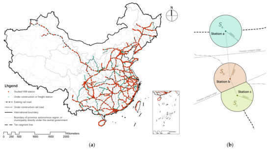
Figure 1.
Study area framework. (a) Spatial distribution of HSR stations across China’s provincial administrative units; (b) Voronoi-adjusted influence zone with 3 km radius buffers.
Previous studies have conventionally defined station influence zones as circular areas with radii ranging from 0.4 to 4.8 km [18]. Chinese scholars typically confine HSR station influence areas within 2–3 km radii [45,46,47]. Our nationwide HSR station samples cover diverse regions in China, including highly developed areas where stations exhibit broader spatial influence [48]. Additionally, policy considerations also necessitate sufficiently large influence ranges: edge effects may distort spatial metrics when analysis zones are too small, as proximity to boundaries compromises measurement validity [49]. This study delineates station influence zones as circular areas with a 3 km radius. To resolve overlapping circular influence zones, we construct Voronoi polygons using HSR stations as discrete nodes. These polygons delineate spatial boundaries that truncate the original 3 km radius circles, with the resultant intersected areas serving as definitive station influence zones (Voronoi-adjusted influence zone, VAIZ), as depicted in Figure 1b.
2.2. Research Framework
The research framework comprises three principal components (Figure 2).
- Multi-source data integration: This study synthesizes multi-source data collected through literature research, including station attribute data, point-of-interest (POI) data, station-area morphological data, socioeconomic data, and ecological data. Following data preprocessing procedures, the raw datasets were systematically categorized and integrated using ArcGIS 10.6 to establish a geodatabase. Through rigorous indicator calculations, characteristic variables for each HSR station were derived, ensuring methodological transparency and analytical reproducibility.
- Dimensionality reduction via BRF-FS: Feature variables underwent robust standardization, with land-use equilibrium indices (land supply capacity and development intensity) serving as target variables. The BRF-FS algorithm compared original features with shadow features to eliminate redundant variables. Cluster optimization analyzed inflection points in within-cluster sum of squares, silhouette coefficients, and Davies–Bouldin index curves. K-means++ clustering was subsequently applied to generate station typology labels using retained features.
- Typology-driven assessment: Cluster labels were integrated with feature variables to derive comprehensive station-specific profiles. Three sequential analyses were executed: (1) cluster evaluation using robust standardized values and feature importance rankings, (2) land-use equilibrium analysis through supply capacity and development intensity diagnostics, and (3) reference interval establishment via normality testing. These analytical dimensions systematically informed feasible development recommendations for station areas.
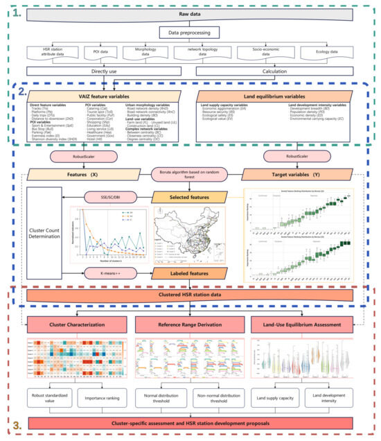
Figure 2.
Methodological workflow: 1. multi−source data integration; 2. dimensionality reduction via BRF−FS; 3. typology−driven assessment.
3. Data
3.1. Raw Data
The systematic categorization of multidimensional datasets within the HSR station VAIZ enhances clustering efficacy and strengthens the reliability of typology-specific threshold reference ranges. Point-of-interest (POI) data, capturing facility classifications and spatial distributions (e.g., category, name, and address) [50,51,52], were sourced from Amap’s 2020 dataset to ensure temporal consistency across all parameters. The HSR network topology data in shapefile format were obtained from the China Railway Network Vector SHP Dataset, enabling spatial pattern analysis through ArcGIS. Urban form refers to the main physical elements that constitute and shape a city [53]. We focus on three core components: road networks acquired from Mapbox (topology-corrected in ArcGIS 10.6), building footprints from Zenodo [54], and land-use data provided by the Data Center for Resources and Environmental Sciences, Chinese Academy of Sciences [55]. Socioeconomic parameters incorporated 2020 demographic data, secondary/tertiary sector GDP, and municipal fiscal revenues of host cities [18,25,56,57,58]. Ecological indicators, while constrained by data resolution limitations, included city-level industrial sulfur dioxide emissions and total water resources to inform sustainability-oriented planning and mitigation design [59]. For the units, detailed descriptions, and data sources, refer to Table 1.

Table 1.
Units, detailed descriptions, and data sources.
3.2. Direct Feature Variable
As critical nodes within the HSR network infrastructure, stations were characterized through four key variables: distance to downtown (DtD), platforms (Pls), tracks (Trs), and passenger volume [37,62]. These direct variables, directly retrievable from official portals such as China State Railway Group Co., Ltd. (CR Group, Beijing, China) without computational processing, were defined as follows: Passenger volume was proxied by daily trips (DTs) due to data accessibility limitations. Platform/track quantities and daily trips were acquired through web scraping of three train schedule portals, and downtown distances were derived from Euclidean distance analysis in ArcGIS 10.6. For detailed information of the direct feature variables, refer to Table 2.
Table 2.
Variable abbreviations, units, detailed descriptions, five-number summary statistics, and data sources of direct feature variables.
3.3. Derived Feature Variable
Derived feature variables were algorithmically generated from raw datasets through formula-based computations. Derived feature variables and the direct feature variables detailed in Section 3.2 collectively constitute the feature set employed in BRF computations. Given the nationwide distribution of HSR stations across China and the critical importance of network attributes, feature reclassification was implemented by integrating POI, urban morphological, and land-use elements augmented with HSR network variables frequently overlooked in small-sample studies. These variables were subsequently evaluated through complex network theory frameworks. For all derived feature variables, including detailed description and references, refer to Table 3. Comprehensive specifications of the derived feature variables, encompassing operational definitions, computational methodologies, and formula interpretations, are systematically elaborated in subsequent sections.
Table 3.
Variable abbreviations, units, detailed descriptions, descriptive statistics, and references of derived feature variables.
3.3.1. POI Variable
Regarding POI data within station areas, as delineated in Section 2.1, the selection of density metrics (versus absolute counts) for POI feature variables was operationalized to address spatial heterogeneity in VAIZ areas across stations [63,64]. Individual POI variables, including the density of catering (Cat), tourist spot (ToS), public facility (PuF), corporation (Cor), shopping (Shp), education (Edu), living service (LiS), healthcare (Hea), government (Gov), hotel (Htl), sport and entertainment (SpE), bus stop (BuS) and parking (Pak), were derived following the classification framework established in Table 1.
This study employs Shannon’s diversity index (SHDI) and the evenness index (EI) to quantify the diversity and distributional equity of Points of Interest (POIs) within station areas. Originally conceptualized in communication theory [65], the information entropy framework has subsequently been employed in cross-disciplinary applications spanning physics, psychology, and biology. As detailed in Table 1, we operationalize SHDI to characterize POI diversity through systematic complexity metrics, where higher index values correspond to greater system complexity and POI diversity. The formula for calculating SHDI is as follows:
where pi denotes the proportion of the i-th POI category relative to the total POI population.
The SHDI attains its theoretical maximum when POI proportions are uniformly distributed across categories, necessitating the introduction of the EI to quantify distributional equilibrium. Scaled between 0 and 1, EI values approaching 1 signify optimal uniformity in POI distributions within the HSR station VAIZ, where categorical proportions exhibit minimal deviation. The computational formalization of EI is expressed as follows:
where N denotes the number of POI categories within the HSR station VAIZ.
3.3.2. Urban Morphology Variable
Building upon Anne Vernez Moudon’s principles of urban morphological analysis and considering data availability, three urban form metrics were adopted at different levels of resolution: lot–block–region [66]. Specifically, building density (BD), road network density (RnD), and road network connectivity (RnC) were selected as morphological descriptors. RnD is calculated as the total length of all road segments within the HSR station VAIZ divided by the VAIZ area. Similarly, BD equals the aggregate building footprint area divided by the VAIZ area. The RnC, a critical indicator of topological maturity and network reliability, quantifies the structural sophistication of regional network systems. The computational formalization in this study is streamlined to accommodate large-scale datasets and is defined as follows:
where N denotes the total number of road network nodes, mi represents the edge count adjacent to the i-th node, and n1, n3, n4, and n5 quantify the aggregate counts of cul-de-sacs, T-junctions, crossroads, and multi-leg junctions, respectively.
3.3.3. Land-Use Variable
Land-use variables are typically excluded due to their overlap with human activity indicators [67,71]. However, in this study covering HSR stations across China, significant differences in local topography, climate, and vegetation across station locations justify their inclusion as supplementary indicators. Based on the land classification method in Section 3.1, these metrics are operationalized as the proportional composition of farm land (FL), construction land (CL), and unused land (UL) relative to the VAIZ area of each HSR station.
3.3.4. Complex Network Variable
Variables within the HSR network were derived from complex network theory [69,70]. The topological variables of HSR stations within the network were quantified using three centrality metrics: degree centrality (DC), closeness centrality (CC), and betweenness centrality (BC). DC measures the number of adjacent nodes to a station, reflecting passenger route choice availability. CC evaluates a station’s average shortest-path distance to all other nodes, indicating its whole network accessibility. BC characterizes a station’s influence by counting its occurrence in all shortest paths between node pairs. These metrics were computed in Pajek3XL with network topology derived from the open-source China Railway Network Vector SHP Dataset mentioned in Section 3.1, ensuring full replicability of the framework [72].
The 2020 China HSR network topology was constructed as a directed graph G = (V, E), where V denotes the set of stations and E represents the set of directed edges. Reflecting the bidirectional operational nature of HSR passenger services, adjacent stations i and j on any HSR line generate two directed edges: edge ei,j from i to j and edge ej,i from j to i (i,j ∈ V), thereby establishing a symmetric adjacency relationship within the asymmetric network structure. This study establishes the computational rule for DC through the following equation:
where wi,j and wj,i denote the weight values of edges ei,j and ej,i, respectively, with wi,j = wj,i = 1 for computational simplification, and n represents the total number of nodes.
The formula for calculating DC is as follows:
where dik denotes the shortest transit distance between nodes i and k.
The calculation of DC is defined by the following equation:
where m and n consist of a node pair in clusters V, σ(m,n) represents the number of shortest paths between nodes m and n, and (m,n|i) is the number of shortest paths between nodes m and n passing through node i.
3.4. Target Variable
In September 2015, the United Nations General Assembly adopted 17 Sustainable Development Goals, among which 7 specifically address land-use optimization to achieve coordinated equilibrium across economic, social, and environmental systems [73]. This study encompasses the entire Chinese HSR network, where stations exhibit marked heterogeneity in climatic regimes, topographic configurations, ecological baselines, and economic development levels. Neglecting this spatial heterogeneity in locational attributes risks formulating development strategies misaligned with station-area land resource endowments. Grounded in spatial supply–demand theory, this research evaluates buffer zone development potential against utilization intensity, establishing a land-use equilibrium metric through the systematic alignment of land supply capacity (LS) and demand intensity (LD). Drawing on existing research and China’s developmental context, LS is characterized through four indices: economic agglomeration (EA), resource security (SG), ecological safety (ES), and ecosystem value (EV). LD is quantified through four indices: development breadth (LB), population density (PD), economic density (ED), and environmental carrying capacity (EC) [74,75,76].
Land provision capacity is constrained by natural, economic, and socio-resource endowments. EA quantifies the economic scale of a station’s host city, while SG evaluates the availability and supporting potential of fundamental resources like water and soil. ES measures the abundance of wetlands, forests, grasslands, and nature reserves, alongside regional ecological security maintenance capabilities. EV represents direct and indirect benefits derived from ecosystem services. LB reflects the spatial scale of regional construction land development. PD directly indicates construction land development intensity. ED measures economic output per unit area, with higher values signifying greater development intensity. EC quantifies industrialization and urbanization impacts on atmospheric and aquatic environments. The units and other detailed descriptions of all target variables are comprehensively provided in Table 4. The built-up LD and LS were calculated using a hybrid approach that integrates arithmetic and geometric averaging. The composite system index is formulated as follows:
Table 4.
Units, detailed descriptions, computational methodologies, and descriptive statistics of target variables.
3.5. Data Visualization
This study selects nine representative zones—northeastern forests, northwestern Gobi, the Beijing–Tianjin–Hebei port, northern grasslands, the Yangtze River Delta, southwest basins, central mountains, the Pearl River Delta, and island–coastal areas—to visualize partial variables across 1018 HSR stations (Figure 3). The results reveal significant variations in characteristic variables both between regions and within individual zones, necessitating categorical classification and quantitative analysis as foundational steps for formulating land-equilibrium strategies in HSR station development.
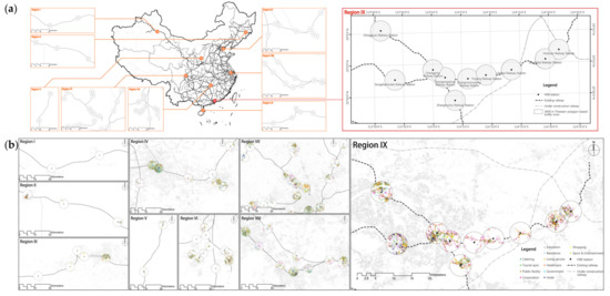
Figure 3.
Spatial patterns of selected variables across nine representative regions. Region designations: I. northwest Gobi; II. northeast forests; III. island–coastal areas; IV. the Beijing–Tianjin–Hebei port; V. northern grasslands; VI. southwest basins; VII. central mountains; VIII. the Yangtze River Delta; IX. the Pearl River Delta. (a) Regional distribution map; (b) POIs; (c) junctions; (d) roads; (e) buildings; (f) population; (g) land-use.
4. Methods
4.1. Dimensionality Reduction
4.1.1. Robust Standardization
Since the variables in Section 3.2, Section 3.3 and Section 3.4 have different measurement units, we standardized the data using robust scaling to make all indicators comparable. As shown in Table 2, Table 3 and Table 4, many variables contained extreme values and uneven data patterns, which make traditional standardization methods unreliable. Robust scaling reduces outlier-induced data distortions while maintaining relative magnitude relationships in empirical distributions [73]. This method replaces mean-based standardization with median-centered normalization and interquartile range (IQR) scaling. Robust standardization using the IQR was implemented to address the outlier sensitivity inherent in traditional methods like Z-score normalization. Given the presence of skewed distributions and numerous outliers in our dataset with substantial value variations across variables, IQR-based standardization provides more stable and reliable standardized results. The formula is as follows:
where Median(X) denotes the central tendency measure of dataset X and IQR(X) is defined as the dispersion measure between the third quartile (Q3) and first quartile (Q1) in X.
4.1.2. Random Forest
This study employs a random forest, a machine learning algorithm initially proposed by Breiman [77], to establish feature importance rankings for HSR station characteristics. Operating through ensemble decision trees with binary splits on predictive variables, the algorithm exhibits computational efficiency and adaptability in handling high-dimensional data with complex variable relationships. By constructing multiple trees using variable subspace sampling at each node, the methodology enhances model generalizability through controlled diversity while mitigating overfitting risks inherent in single-tree models. The HSR station samples exhibit high-dimensional features. RF algorithm eliminates the need for VIF diagnostics to address multicollinearity among features, thereby significantly streamlining methodological procedures. Compared with other ensemble algorithms, the RF demonstrates superior predictive accuracy, enhanced noise resistance, reduced parameter tuning complexity [78], lower computational costs, and minimized overfitting risks. RFs have been described as adaptive nearest-neighbor estimators because they select predictors [79]. Considering its synergy with the Boruta algorithm [80], the RF serves as the foundational model for deriving feature importance rankings.
4.1.3. Boruta Algorithm
The Boruta algorithm is a wrapper method for feature selection specifically designed to identify statistically significant features critical to predictive models within datasets. Its operational framework employs an iterative approach to evaluate feature importance through the following procedure: (1) the replication of the original feature set with randomized permutations of each feature’s values to construct stochastic shadow features; (2) the integration of original features and shadow features into a composite training dataset; and (3) an iterative comparison of importance scores between original and shadow features during each RF cycle, thereby enabling the systematic identification of optimal feature subsets for modeling [43]. The algorithm quantifies importance using the Z-score metric, where a random permutation of feature values induces classification accuracy loss. The Z-score is expressed as the ratio of the mean accuracy loss to its standard deviation, with the formula defined as follows:
where MSEOOB denotes the out-of-bag error of the RF model, yi is the observed value, ŷiOOB is the predicted value for the out-of-bag samples of observation yi, and N is the sample size.
where Zscore denotes the Z-score, represents the mean out-of-bag error, and SDMSEOOB denotes the standard deviation of out-of-bag errors.
To address the substantial value ranges and prevalent outliers across variables, robust scaling was applied to all variable values. Features from Section 3.2 and Section 3.3 were designated as input variables (X), while LS and LD in Section 3.4 served as target variables (y). The dataset was partitioned into 80% training and 20% testing subsets using stratified random sampling. A random forest classifier was initialized for feature importance evaluations, with BRF-FS conducted through iterative comparisons against shadow features over 100 bootstrap iterations. This process generated Z-score rankings that quantify each feature’s discriminative power. Final feature selection excluded statistically irrelevant predictors based on Boruta’s classification (confirmed/tentative/rejected).
4.2. K-Means++ Clustering Algorithm
The K-means algorithm represents a prominent clustering method in data mining, as it is renowned for its computational efficiency. However, its implementation encounters two principal constraints: the random initialization of cluster centroids and suboptimal convergence rates [81]. The K-means++ variant addresses these limitations by optimizing centroid selection through distance-based initialization protocols [82]. This improved algorithm sequentially determines initial centers by identifying data points with maximum and minimum distances to existing centroids, effectively reducing clustering redundancy while enhancing operational stability, an approach particularly suited for analyzing high-dimensional urban rail transit datasets.
The implementation of K-means++ requires a predefined number of clusters (k), which were determined through the integrated evaluation of three metrics: the sum of squares due to an error (SSE), the silhouette coefficient (SC), and the Davies–Bouldin index (DBI). SSE quantifies intra-cluster cohesion, where lower values indicate tighter data aggregation around centroids and improved clustering quality. The metric is calculated as follows:
where Ci denote the sample set of the i-th cluster, k denotes the total number of clusters, p represents a sample within a cluster, and is the squared distance between sample p and the centroid ci of the i-th cluster.
SC measures clustering quality by evaluating intra-cluster cohesion and inter-cluster separation. This metric calculates the balance between minimized within-cluster distances and maximized between-cluster distances, with values ranging from −1 to 1. Higher SC values indicate superior clustering effectiveness, providing quantitative validation for spatial pattern analysis in urban infrastructure studies.
where n denotes the total number of data points in dataset C, ap represents the mean intra-cluster distance between sample p and all other samples within its assigned cluster, and bp denotes the mean nearest-cluster distance quantifying separation from samples in the closest adjacent cluster.
DBI assesses clustering quality by computing the average similarity between each cluster and its most comparable adjacent cluster. This metric defines cluster similarity as the ratio of summed intra-cluster diameters to inter-cluster distances, where lower DBI values correspond to superior clustering outcomes by minimizing inter-cluster similarity. The evaluation mechanism demonstrates particular efficacy, with optimal clustering solutions approaching minimal index values.
where si represents the within-cluster diameter (average distance between samples and the centroid in the i-th cluster) and corresponds to the distance between the centroids of clusters i and j.
4.3. Threshold Reference Range Analysis
To operationalize clustering insights for strategic development, this study defines reference intervals for station-area variables through statistically validated criteria. The methodology first conducts Shapiro–Wilk normality testing on cluster-specific samples. Non-significant results (p > 0.05) confirmed the normal distribution, while samples with absolute kurtosis and skewness values below 2 were explicitly classified as approximately normal and treated as normally distributed [83]. Building on clinical medicine’s reference value protocols [84], a dual-criterion reference framework was developed according to data distribution characteristics:
- For samples exhibiting normal or approximately normal distributions, the parameter settings of the probability interval were determined as (μ − σ, μ + 2σ) to achieve a normal distribution probability of 83.9% [85], considering the specific developmental characteristics and functional requirements of the research subject. This interval design addresses bidirectional control needs in planning indicators, thereby maintaining flexibility for positive development while establishing baseline thresholds. Subject to parameter value ranges, the upper and lower bounds of the reference range may require subsequent adjustments. Specifically, variables with a value range ≥ 0 but exhibiting a fitted lower bound <0 had their reference intervals modified to [0, μ + 2σ) accordingly.
- For samples with non-normally distributed data, the reference ranges of skewed distribution parameters were determined using non-parametric methods (P13.5–P97.5) while maintaining conceptual alignment with the probability intervals established for normal or approximately normal distributions.
Based on these criteria, preliminary indicator ranges for each cluster were subsequently established. The final reference value ranges were derived through the systematic integration of land development intensity analysis and land supply capacity assessments, combined with urban development pattern examination and indicator characteristic evaluations across clustered site categories. This differentiated reference value system for construction indicators according to station typologies facilitates the precise regulation of urban renewal processes in existing station areas and design progression control in new station developments. The methodology enhances urban land utilization efficiency while promoting high-quality spatial development in station-adjacent territories.
5. Results
5.1. BRF-FS Results
This study conducted iterative Boruta algorithm executions to evaluate feature ranking stability under two target variables: land supply capacity (LS) and land development intensity (LD). The visualization of ranking consistency in Figure 4 reveals distinct patterns, where left-positioned features such as construction land and road connectivity demonstrate persistent high rankings across iterations, confirming their model’s significance. Conversely, right-aligned features including shopping POI and degree centrality exhibit lower ranking stability, suggesting relatively diminished predictive value in our analytical framework.
Figure 4.
Sorted feature ranking distribution by Boruta. (a) LS; (b) LD.
Detailed classification outcomes, including confirmed features, tentative features, and rejected features with corresponding ranking positions, are systematically cataloged in Table 5. Previous studies have integrated LS and LD to comprehensively assess land-use patterns [79]. In alignment with land development equilibrium (DS variable) methodologies that integrate LD and LS assessments, the union of confirmed and tentative features from both target variable configurations yielded 11 critical determinants: Cat, Cor, SpE, BuS, RnD, RnC, FL, CL, UL, Pls, and DtD. These validated features will serve as dimensional anchors for subsequent cluster analysis phases. Building upon established methodologies that integrate LS and LD assessments, this study selects the union of confirmed and tentative features from both indicators as critical determinants. This approach maintains methodological continuity with conventional land-use evaluation frameworks while optimizing feature selection through cross-indicator validation.
Table 5.
Final rankings and BRF-FS outcomes, categorizing variables into three classifications: confirm (C, green shading), tentative (T, yellow shading), and rejected (R, red shading).
5.2. Clustering Results
The K-means++ algorithm’s evaluation metrics demonstrate definitive clustering characteristics at k = 9, as illustrated in Figure 5. The SSE curve exhibits convergence initiation with marked deceleration in the decline rate, while the SC attains peak values, and the DBI reaches its minimum range. This multi-criteria optimization framework confirms the validity of partitioning 1018 HSR rail stations into nine distinct clusters.
Figure 5.
Cluster-dependent evaluation metric curves.
Geospatial analysis reveals significant locational differentiation (Figure 6): Clusters 1, 6, and 9 predominantly occupy core urban agglomerations; Clusters 2, 3, 5, and 7 concentrate in peri-urban zones of metropolitan areas or county-level suburbs; Cluster 4 stations predominantly situate in township-level suburban or rural–urban fringe areas.
Figure 6.
Spatial distribution of HHSR stations in each cluster. (a) Overall distribution; (b) Cluster 1; (c) Cluster 2; (d) Cluster 3; (e) Cluster 4; (f) Cluster 5; (g) Cluster 6; (h) Cluster 7; (i) Cluster 8; (j) Cluster 9.
6. Discussion
6.1. Cluster Characterization
Further analysis was conducted on all clusters through a heatmap visualization of characteristic indicators, which details the core metric features of HSR stations across clusters. This analytical framework implemented robust standardization to process multidimensional indicators, thereby preserving original distribution characteristics while neutralizing dimensional units and mitigating outlier impacts, features critical for evaluating nationally distributed HSR stations with heterogeneous development patterns. As visualized in Figure 7, the heatmap employs orange-to-teal color gradients where normalized mean values approaching 3 (red) indicate cluster-specific metric superiority, while values near −1 (blue) reflect relative underperformance. Subsequent cross-validation with raw datasets enabled the systematic categorization of nine station clusters, revealing distinct development typologies that inform differentiated land-use optimization strategies.
Figure 7.
Heatmap visualization of robustly standardized mean values for cluster-specific characteristic metrics.
Cluster 1: Secondary Service-Anchored HSR Stations. These stations serve as regional transit hubs (11.63 Trs and 127.13 DTs) with marginal network influence (BC: 0.016). High urbanization intensity (75.36% CL) clusters reveal basic amenities (LiS: 23.86/km2; Hea: 8.34/km2), while commercial (6.59/km2) and cultural–tourism facilities (0.48/km2) remain underdeveloped. Multimodal capacity combines parking (14.10/km2) and road networks (8.97/km2), balancing high functional equilibrium (0.84) with low diversity (0.42). Representative HSR stations include Baotoudong, Qiqihar, Tongliao, etc.
Cluster 2: Peripheral Basic-Commercial HSR Stations. These stations demonstrate moderate operations (6.55 Trs, 85.32 DTs) with peak commercial density (35.1/km2) amid suburban–agricultural transition zones. Farm land dominates (48.9%) alongside limited urbanization (25.55% CL), while weak public transit (0.77/km2) and mid-range closeness centrality (0.038) reveal accessibility constraints. Low functional diversity (0.73) highlights imbalanced development where commercial clustering exceeds supporting service maturation, creating polarized corridors along rail routes. Representative HSR stations include Lilingdong, Baise, Jieyang, etc.
Cluster 3: Enterprise-Intensive Monofunctional HSR Stations. These stations functions as specialized enterprise hubs (38.47/km2, highest) with paradoxically low service frequency (65 DTs). It maintains critical network accessibility (CC: 0.040, peak) while exhibiting severe civic amenity deficiencies (Pak: 0.72/km2). Farm land predominance (45.26%) coexists with fragmented urbanization (30.69% CL), compounded by inadequate transit integration (BuS: 0.79/km2). Representative HSR stations include Lankaonan, Jinzhong, Yunxiao, etc.
Cluster 4: Agri-Dominant Underdeveloped HSR Stations. This cluster exhibits underdeveloped transport characteristics with constrained rail infrastructure capacity (4.97 Trs and 46.66 DTs) and minimal functional diversity (index: 0.231), reflecting service specialization in single-sector operations. The spatial configuration demonstrates rural predominance, with agricultural land cover reaching 53.90% and limited urban development (10.80% CL). These nodes display distinct peripheral growth trajectories, characterized by low-density settlement patterns and agricultural economic bases. Representative HSR stations include Yongjibei, Heishanbei, Mile, etc.
Cluster 5: Suburban-Supported Commercial HSR Stations. These stations establish themselves as the dominant commercial hub (36.16/km2, highest) with mid-level rail infrastructure (6.65 Trs, 86.29 DTs). Land use reflects suburban transition (34.16% CL vs. 39.65% FL), while parking inadequacy (2.27/km2) contradicts robust road network connectivity (2.89). This configuration creates hybrid stations that excel in commercial activities yet struggle with multimodal integration. Representative HSR stations include Yiwu, Deyang, Tongling, etc.
Cluster 6: Metropolitan Core Hub HSR Stations. These stations function as national rail pivots, processing peak traffic (13.94 Trs and 315.44 DTs) in near-total urbanization (94.42% CL). Multimodal efficiency achieves seamless integration via dense road systems (16.03/km2) and unparalleled parking capacity (52.22/km2, 7.3 × Cluster 5). Paradoxically, basic service provision stagnates, and catering (16.29/km2) and life services (16.83/km2) operate at merely 42–48% of Cluster 9’s levels, exposing a critical imbalance between mobility infrastructure and user-centric amenities. Representative HSR stations include Guangzhoudong, Taibei, Hangzhou, etc.
Cluster 7: Balanced Regional Service HSR Stations. These stations serve as secondary mobility hubs, processing moderate rail volumes (6.34 Trs and 91.93 DTs) with balanced functional provision. Cultural–tourism infrastructure (1.16/km2) outperforms peer clusters, yet multimodal connectivity is hindered by parking deficiencies (1.81/km2) and sparse road networks (3.77/km2). Suburban land configurations dominate (33.43% CL and 43.61% FL), where commercial (24.20/km2) and life services (11.29/km2) underperform relative to urban stations. Representative HSR stations include Hainingxi, Lugu, Dongjiakou, etc.
Cluster 8: Remote Transit Accommodation HSR Stations. These stations are characterized as remote suburban hubs (60.09 km DtD), processing moderate rail traffic (6.79 Trs and 74.39 DTs). Elevated catering (28.73/km2) and life services (20.89/km2) contrast with underdeveloped commercial (10.45/km2) and cultural–tourism infrastructure (0.68/km2). Multimodal integration remains suboptimal despite moderate road density (3.15/km2), exacerbated by critical parking shortages (0.94/km2), and it is merely 16% of Cluster 6’s capacity. Representative HSR stations include Zhaodong, Dtongxi, Weihexi, etc.
Cluster 9: Commercial-Intensive Hub HSR Stations. These stations operate as major rail hubs (11.86 Trs and 232.88 DTs) in proximity to urban cores (10.31 km DtD). High urbanization intensity (81.26% CL) supports commercial prominence (35.45/km2), while cultural–tourism provisions are critically low (0.40/km2). Multimodal accessibility is maintained through substantial parking (16.93/km2) and dense road infrastructure (9.65/km2). Representative HSR stations include Shenzhenbei, Xiangtan, Suzhouxi, etc.
Current cluster-specific analyses predominantly focus on explicit features like built environment patterns, transport networks, and passenger flows while insufficiently addressing the developmental potential assessment of socio-economic ecosystems within station influence zones. The uncritical adoption of uniform planning frameworks and standardized policy instruments, particularly when implemented without rigorous consideration of localized land-use constraints and established development intensity thresholds, may be exacerbated by systematic resource allocation mismatches. Such planning oversights frequently manifest as spatial–functional disarticulation, ecological vulnerability escalation, and station-centered service provision inequalities. To address this gap, a systematic evaluation of land development intensity and land supply capacity becomes essential for guiding adaptive development strategies.
6.2. Land-Use Equilibrium Assessment
This study employs raincloud plots to visualize the LS-LD distribution patterns. The bilateral half-density curves, derived through kernel density estimation, precisely characterize data distribution morphology, outperforming traditional histograms in probability density representation. Central jittered scatterplots preserve raw data point distributions, while embedded boxplots quantify central tendencies (medians and interquartile ranges) and outlier distributions. The integrated visualization framework enables the comparative analysis of LS-LD density variations across clusters. The side-by-side raincloud plots visually compare LS-LD distributions across clusters. This integrated visualization identifies typical development–supply mismatches through median line connections, including high LS–low LD, low LS–high LD, etc.
As illustrated in Figure 8, Clusters 1, 6, and 9 exhibit significant supply–development imbalances where land supply capacity substantially lags behind development intensity, necessitating development pace control and ecological preservation in subsequent planning interventions. Cluster 4 demonstrates inverse characteristics with underutilized supply potential, requiring integrated compact development strategies while maintaining alignment with regional economic carrying capacities to prevent resource misallocation. Clusters 2, 3, 5, and 7 show moderate supply surpluses relative to development levels, indicating untapped resource potential that demands efficiency-driven development optimization based on the findings in Section 6.1. Cluster 8 maintains the most balanced land utilization as it is closest to sample-wide median levels, though sub-indicator analysis reveals approaching saturation in resource security reserves coupled with economic agglomeration deficiencies, necessitating functional repositioning strategies to activate existing resource value. The raincloud plots further identify bimodal polarization patterns in land supply capacity for Clusters 3 and 6, necessitating differentiated development strategies for these polarized subgroups.
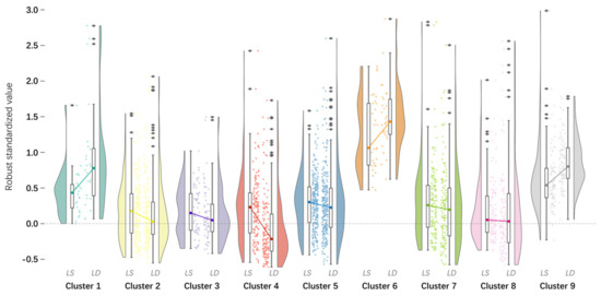
Figure 8.
The LS-LD cloud diagram for HSR stations in each cluster. The endpoints of the connecting lines in each cluster’s box plot are the normalized mean values of the LS and LD values.
It should be emphasized that the equilibrium assessment represents cluster-level trends, while site-specific strategies must account for individual station characteristics. Strategic recommendations derive from these spatial resource allocation patterns are as follows: For clusters demonstrating critical land supply deficits relative to development intensity, the implementation of development pace regulation and ecological preservation measures becomes imperative. Clusters with underutilized land provision capacities require compact, polycentric development models aligned with regional economic carrying capacities to prevent resource misallocation. Moderately mismatched clusters warrant efficiency-oriented interventions informed by the cluster-specific analyses detailed in Section 6.1. The balanced development cluster demands a granular examination of LS and LD sub-indicators (Table 4) to identify potential optimization pathways.
6.3. Cluster-Specific Threshold Reference Ranges
Variable screening preceded the determination of threshold reference ranges. Station-specific metrics including Pls, Trs, DTs, and DtD were excluded from analysis as they fall beyond the scope of HSR station influence zone development planning. Given the established mathematical derivation between SHDI and EI (see Equation (2) where N = 14), the former was retained. Shapiro–Wilk normality test results for each cluster are presented in Table 6, following the methodology detailed in Section 4.3.
Table 6.
Final rankings and sorted results of all feature variables.
Table 6 shows that most of the samples of Cat and Shp conform to a normal distribution because they are closely related to the basic needs of travelers, and the upper limit of the scale of these businesses is limited by demand, so most of them are concentrated in the middle range. Most of the samples of Htl, PuF, and ToS do not conform to the normal distribution, because the resource endowment of each site area has a large gap, which is reflected in the level of land development and utilization, and there may be a serious imbalance between land development and land supply in the areas where each site is located. The development suggestions made by previous studies only through the preliminary cluster analysis of the sites may not have a high reference value, which is one of the reasons why this study introduces the theory of land supply and demand to enrich the development suggestions.
The existing urban design indicator system has established a fundamental threshold framework (e.g., universal ranges such as a floor area ratio of 1.5–2.5 and a green space ratio of 15–20%) yet demonstrates significant limitations in station-specific adaptability. Standardized reference values prove inadequate to accommodate differentiated urban development patterns and local ecological–economic capacities across diverse HSR station areas. Multi-source data fusion analysis of 1018 Chinese HSR station areas reveal substantial variations: Agri-Dominant Underdeveloped HSR Station areas achieve acceptable performance, with the road network density ranging from 0.58 to 4.98 km/km2, while Metropolitan Core Hub HSR Station areas require significantly higher density parameters between 12.74 and 21.47 km/km2. Reference ranges for other characteristic elements are detailed in Figure 9. The machine learning-driven differential benchmarking mechanism provides urban design decision systems with scalable modular tools while offering clear parametric guidance for station areas undergoing strategic transformation. It should be emphasized that the reference interval system functions as a flexible regulatory mechanism rather than a rigid control standard. Consequently, indicators at specific sites falling below the lower bound or exceeding the upper bound of their categorical reference ranges do not inherently indicate inferior or superior performance, as this framework intentionally accommodates contextual variations through its adaptive threshold design.
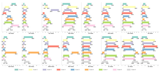
Figure 9.
Reference ranges for indicators by cluster.
This study employs a random forest method based on the Boruta algorithm, which demonstrates unique advantages in multi-modal feature cluster analysis. The RF is more computationally efficient on a tree-by-tree basis since the tree-building process only needs to evaluate a fraction of the original predictors at each split, although more trees are usually required by random forests. Combining this attribute with the ability to parallel process tree building makes random forests more computationally efficient than boosting [86]. Compared with the linear assumption of spatial heterogeneity and the limitation of single-scale analysis in the multiscale geographically weighted regression (MGWR) model, the random forest algorithm integrated with Boruta feature selection can capture the complex interaction relationships among the multi-modal features of high-speed railway stations through a multi-decision-tree voting mechanism. However, this approach also has several potential limitations: While robust to noise and collinearity, excessive spatial heterogeneity in station distributions may weaken the local characteristics in the global model under default Bagging sampling [87]. Additionally, the black-box nature reduces cluster boundary interpretability, hindering the intuitive revelation of causal links between multi-modal features and clustering characteristics.
6.4. HSR Station Area Development Strategies
By comprehensively considering the indicator characteristics, land supply capacity, and development intensity of each station cluster, this study diagnoses the key contradictions and risk warning of the HSR station clusters and proposes the following development strategies:
Secondary Service-Anchored HSR Stations: Because of the HSR network limitations, these stations show a systemic mismatch between high transportation capacity and low BC, which are mostly used as terminal stations on feeder lines. Even though they are in central areas, they have little functional diversity because of their limited retail space, which results in underleveraged passenger volumes resulting from lower commercial appeal. Extended vacancy of undeveloped land parcels may exacerbate spatial segregation around stations, highlighting the possibility of underestimating the potential for land appreciation. In order to increase nodal relevance within railway networks and improve multimodal feeder systems, future development should place a higher priority on building new inter-regional trunk lines. In view of the shortage of land, underground spaces (the underground retail corridors of the Osaka–Umeda Station) may be used for both commercial and hospitality purposes. In order to promote precinct regeneration and to ensure balanced spatial development around transport hubs, the current land that is being used should be designated as protected green spaces.
Peripheral Basic-Commercial HSR Stations: These stations show high commercial density but suffer from poor healthcare and basic services provision due to poor accessibility that limits sustained passenger retention. Thus, overreliance on typical retail formats jeopardizes increasing vacancy rates. Interventions should focus on financially balanced measures, such as introducing fast transit corridors (e.g., BRT) to increase downtown connectivity and developing park-and-ride facilities to convert passenger flow into local commercial patronage. For stations serving populous townships, establishing low-cost community hubs with integrated essential service centers might stabilize their footprint while addressing resident service gaps. In places with strong enterprise clustering and adequate municipal fiscal capacity, building SME procurement centers or co-working commercial complexes may prove feasible.
Enterprise-Intensive Monofunctional HSR Stations: These stations exhibit the highest CC and enterprise density within the network yet demonstrate underutilized transport value due to low DTs. The overconcentration of manufacturing industries may trigger sectoral decline during industrial transitions. Strategic development should align with municipal fiscal capacity and statutory planning frameworks. For stations with sufficient land supply capability, UL could be allocated to social security housing and community clinics, with partial FL converted into urban agriculture demonstration zones. Conversely, in areas with low land supply capacity, the adaptive reuse of existing industrial facilities, such as retrofitting warehouses into logistics hubs or SME workspaces, should be prioritized. Streamlining land-use conversion procedures for these precincts can optimize spatial functions without costly redevelopment.
Agri-Dominant Underdeveloped HSR Stations: These stations show suboptimal locational characteristics and UL, characterized by agri-residential amalgamations despite apparent mixed-use intensity. The lack of transport infrastructure and coordinated planning frameworks has resulted in defective spatial arrangements. The indiscriminate reproduction of urban development models implies facility redundancy because of low demand, probably encroaching on ecological preservation zones and triggering municipal debt burdens. Strategies should focus on context-specific interventions, such as establishing rural–urban logistics hubs or agri-education hubs where possible, with limited service facilities (e.g., agricultural supply centers and community clinics) permitted outside protected farmland through allotted construction quotas. Aligned with statutory planning hierarchies, devoted rural transit routes or upgraded cycling corridors using existing village pathways should be adopted to increase last-mile connectivity.
Suburban-Supported Commercial HSR Stations: These stations show moderate DTs but severely low CC, making them unreliable for converting transport scale into network value. Despite showing strong commercial services and public amenities with better roadway connectivity, many suffer from inadequate transit provision. Strategic development should take advantage of residual land potential through integrated community commerce and wellness-oriented amenities, complemented by regional markets where possible. Existing roadway capacity might be repurposed for dedicated bus lanes to increase public transport modal share, whereas transforming UL into pocket parks might improve residential quality and ecological capital by targeted green infrastructure deployment.
Metropolitan Core Hub HSR Stations: These high-traffic locations encounter important difficulties in integrating extremely dense development with ecological carrying capacity, necessitating vertical functioning variety and the protection of public places from excessive commercialization. Future solutions should use frontier technologies, including AI-driven analytics, IoT-enabled systems, and low-altitude drone logistics, to increase service efficiency and integrated three-dimensional spatial controlled dynamics. For stations with high land supply capability, exploration for mid/deep-level underground space development models is advised. Conversely, stations with low supply capability should maintain vertical ecological retrofitting through biophilic design interventions, avoiding over-built buffer greenbelts that compromise community well-being.
Balanced Regional Service HSR Stations: These stations demonstrate submedian performance in Shp, Cor, and PuF yet retain modest enterprise clustering. Predominantly located at suburban peripheries with minimal public transit coverage, strategic interventions should prioritize blended industry–residential systems through low-capital initiatives such as corporate consortium-operated commuting shuttles and lunchtime marketplaces. Basic guaranteed transit routes must ensure mobility equity for essential trips. Incremental endogenous service capacity building should be pursued during fiscally constraint periods. The government should implement adaptive land-use frameworks to deploy micro-service modules (e.g., employee housing units and compact fitness centers) contingent on municipal fiscal capacity while converting underutilized parcels into designated green buffers.
Remote Transit Accommodation HSR Stations: These stations exhibit the longest DtD and are predominantly located in county towns or suburban peripheries but are partially offset by superior public transit accessibility. Characterized by high catering density, moderate essential service provision, and low commercial intensity, persistent inadequacies in public service upgrades may exacerbate hollowing-out effects due to youth migration toward metropolitan centers. Strategic interventions should focus on place-specific service enhancement and attraction mechanisms through three integrated pathways: (1) leveraging transit connectivity to establish rural–urban service hubs, (2) extending consumption chains via the temporal zoning of dining clusters (e.g., daytime retail to nighttime cultural markets), and (3) activating underutilized land for wellness-oriented infrastructure to strengthen rural catchment retention, thereby mitigating depopulation risks through targeted spatial revitalization.
Commercial-Intensive Hub HSR Stations: These stations are characterized by proximity to urban cores; however, because of their locational advantages, they do not always result in high functional diversity, which shows a low level of public service provision but a high commercial density. Subsequent approaches ought to place a strong emphasis on transit-oriented integrated development via vertical mixed-use complexes and improved subterranean spatial utilization. The current infrastructure gaps would be addressed by the planned placement of modular public service units inside station areas. The capitalization of current green spaces should include the connectivity of transit nodes with residential clusters via the pedestrian–cyclist networks, thereby increasing multimodal accessibility while maintaining ecological integrity.
Traditionally, there is a problem in the way that decision-makers mechanically replicate established station-area models, which are typically not adjusted to local land capacity thresholds; this is a common problem that frequently results in mismatches between the capacity of land supply and development intensity. The purpose of this study is to prevent structural differences between planning visions and operational realities, which result in underutilized “ghost stations”, which are a result of significant financial strain and resource waste in order to address balanced land-use strategies for HSR station areas. Our statistical model sets reference value ranges that prioritize flexible performance standards over rigid constraints, which in turn requires adaptive planning frameworks to take into account dynamic urban transitions.
Notably, the 2020 study sample—Pu’an Station (Cluster 7, Wuhan, China)—was decommissioned in 2022 [88]. This case precisely matches our characterization of Cluster 7 station areas: within its VAIZ, numerous corporate campuses and industrial parks coexist, yet the area lacks metro connectivity and adequate bus services, with the nearest bus stop requiring a 15 min walk. Local policymakers failed to leverage adjacent academic–industrial resources or guarantee basic public transit, resulting in low endogenous service capacity and insufficient passenger demand despite proximity to universities and residential communities. The station’s closure resulted from three intersecting pressures: persistent ridership shortages, adjustments to regional planning frameworks, and tightening local fiscal constraints. The closure of Pu’an Station validates the disconnect between station-area land development and land supply capacity.
7. Conclusions
Integrating economic principles with multidimensional socioeconomic development factors enhances spatial equilibrium analysis in land-use planning. This approach considers the common supervision in the available literature and engineering practices that focus construction metrics and best prototypes while neglecting detailed station-area measurements. Our study uses a BRF to separate the development priorities of HSR stations under the combined influences of built environments, HSR network topology, local ecology, and economic dynamics. Enhanced clustering algorithms classify station typologies, generating cluster-specific development strategies and quantitative reference ranges guided by land-use equilibrium theory, thus establishing adaptive planning frameworks. The Boruta algorithm shows overlap between verified/tentative features when separately modeling land supply capacity and development intensity as target variables. All land-use variables (FL, CL, and UL) and road network variables (RnD and RnC) were identified as critical discriminators of station-area land-use equilibrium. Platforms (Pls) and the distance to downtown (DtD) further show significant classification power in HSR station typologies.
This research advances the discourse through pan-regional analysis encompassing all operational Chinese HSR stations. Cross-comparative examinations incorporating mature European station development paradigms and Southeast Asian cases could substantively enhance the theoretical robustness of proposed planning frameworks.
This study’s development recommendations and numerical reference ranges serve as directional guidance for HSR rail station planning, requiring contextual adaptation to local conditions during implementation. Further research could focus on investigating the spatiotemporal heterogeneity of station-area characteristics, for example, through longitudinal analyses of land equilibrium utilization patterns using expanded datasets spanning 2000 to 2020. Methodological improvements could involve the spatial stratification of station influence areas by establishing concentric buffers at 0–1 km, 1–2 km, and 2–3 km radii, enabling the granular analysis of development intensity gradients across micro-scale zones. Such refinements would address current limitations in capturing localized development disparities while maintaining theoretical consistency with land supply–demand equilibrium principles.
Author Contributions
Conceptualization, X.L. and H.Y.; methodology, X.L. and F.Z.; software, X.L.; validation, Z.L., R.D. and Y.W.; formal analysis, X.L.; investigation, Y.W., Z.Q. and Y.G.; resources, X.L., H.Y. and Y.W.; data curation, X.L., F.Z. and Z.L.; writing—original draft preparation, X.L.; writing—review and editing, X.L., F.Z. and H.Y.; visualization, X.L.; supervision, X.L., F.Z. and H.Y.; project administration, X.L. and H.Y.; funding acquisition, H.Y. All authors have read and agreed to the published version of the manuscript.
Funding
This research was funded by Sichuan International Science and Technology Innovation Cooperation/Hong Kong, Macao and Taiwan Science and Technology Innovation Cooperation Project (NO. 2024YFHZ0220); 2022 General Project of Humanities and Social Sciences Research of the Ministry of Education (NO. 22YJCZH226).
Data Availability Statement
Data presented in the study in Section 3.2 and Section 3.3 are openly available at https://kdocs.cn/l/cduPyVLGVijR (accessed on 28 April 2025). Other data are available upon request to the corresponding author due to their large volume.
Conflicts of Interest
The authors declare no conflicts of interest.
Abbreviations
The following abbreviations are used in this manuscript:
| HSR | High-speed railway | TOD | Transit-oriented development |
| GIS | Geographic information systems | BRF-FS | Boruta–random forest feature selection |
| RF | Random forest | VIF | Variance inflation factor |
| POI | Point of interest | VAIZ | Voronoi-adjusted influence zone |
| UIC | International Union of Railways | DtD | Distance to downtown |
| Pls | Platforms | Trs | Tracks |
| Cat | Catering | ToS | Tourist spot |
| PuF | Public facility | Cor | Corporation |
| Shp | Shopping | Edu | Education |
| LiS | Living service | Hea | Healthcare |
| Gov | Government | Htl | Hotel |
| SpE | Sport and entertainment | BuS | Bus stop |
| Pak | Parking | SHDI | Shannon diversity index |
| EI | Evenness index | BD | Building density |
| RnD | Road network density | RnC | Road network connectivity |
| FL | Farm land | CL | Construction land |
| UL | Unused land | DC | Degree centrality |
| CC | Closeness centrality | BC | Betweenness centrality |
| LS | Land supply capacity | LD | Land demand intensity |
| EA | Economic agglomeration | RS | Resource security |
| ES | Ecological safety | EV | Ecosystem value |
| DB | Development breadth | PD | Population density |
| ED | Economic density | EC | Environmental carrying capacity |
| IQR | Interquartile range | SSE | Sum of squares due to an error |
| SC | Silhouette coefficient | DBI | Davies–Bouldin index |
References
- Ahlfeldt, G.M.; Feddersen, A. From Periphery to Core: Measuring Agglomeration Effects Using High-Speed Rail. J. Econ. Geogr. 2018, 18, 355–390. [Google Scholar] [CrossRef]
- Ke, X.; Chen, H.; Hong, Y.; Hsiao, C. Do China’s High-Speed-Rail Projects Promote Local Economy?—New Evidence from a Panel Data Approach. China Econ. Rev. 2017, 44, 203–226. [Google Scholar] [CrossRef]
- Yang, X.; Zhang, H.; Lin, S.; Zhang, J.; Zeng, J. Does High-Speed Railway Promote Regional Innovation Growth or Innovation Convergence? Technol. Soc. 2021, 64, 101472. [Google Scholar] [CrossRef]
- Wang, C.; Chen, J.; Li, B.; Chen, N.; Wang, W. Impact of High-Speed Railway Construction on Spatial Patterns of Regional Economic Development Along the Route: A Case Study of the Shanghai–Kunming High-Speed Railway. Socio-Econ. Plan. Sci. 2023, 87, 101583. [Google Scholar] [CrossRef]
- Amos, P.; Amos, P.; Bullock, D.; Sondhi, J. High-Speed Rail the Fast Track to Economic Development? World Bank: Washington, DC, USA, 2010. [Google Scholar]
- CGTN China-Built Jakarta-Bandung High-Speed Railway Begins Operation 2023. Available online: https://news.cgtn.com/news/2023-10-18/China-built-Jakarta-Bandung-high-speed-railway-begins-operation-1o0a68je8rm/index.html (accessed on 4 September 2024).
- Shen, Q.; Pan, Y.; Feng, Y. The Impacts of High-Speed Railway on Environmental Sustainability: Quasi-Experimental Evidence from China. Humanit. Soc. Sci. Commun. 2023, 10, 719. [Google Scholar] [CrossRef]
- Dong, L.; Du, R.; Kahn, M.; Ratti, C.; Zheng, S. “Ghost Cities” Versus Boom Towns: Do China’s High-Speed Rail New Towns Thrive? Reg. Sci. Urban Econ. 2021, 89, 103682. [Google Scholar] [CrossRef]
- Zheng, L.; Long, F.; Chang, Z.; Ye, J. Ghost Town or City of Hope? The Spatial Spillover Effects of High-Speed Railway Stations in China. Transp. Policy 2019, 81, 230–241. [Google Scholar] [CrossRef]
- Salvati, L.; Serra, P. Estimating Rapidity of Change in Complex Urban Systems: A Multidimensional, Local-Scale Approach. Geogr. Anal. 2016, 48, 132–156. [Google Scholar] [CrossRef]
- Zhang, G.; Zheng, D.; Wu, H.; Wang, J.; Li, S. Assessing the Role of High-Speed Rail in Shaping the Spatial Patterns of Urban and Rural Development: A Case of the Middle Reaches of the Yangtze River, China. Sci. Total Environ. 2020, 704, 135399. [Google Scholar] [CrossRef]
- Zhang, C.; Xia, H.; Song, Y. Rail Transportation Lead Urban Form Change: A Case Study of Beijing. Urban Rail Transit 2017, 3, 15–22. [Google Scholar] [CrossRef]
- Sun, X.; Yan, S.; Liu, T.; Wu, J. High-Speed Rail Development and Urban Environmental Efficiency in China: A City-Level Examination. Transp. Res. Part D Transp. Environ. 2020, 86, 102456. [Google Scholar] [CrossRef]
- Cheng, J.; Hu, L.; Zhang, J.; Lei, D. Understanding the Synergistic Effects of Walking Accessibility and the Built Environment on Street Vitality in High-Speed Railway Station Areas. Sustainability 2024, 16, 5524. [Google Scholar] [CrossRef]
- Xia, X.; Li, H.; Wang, K.; Liu, Y. Analysis of the Impact of High-Speed Rail on the Spatio-Temporal Distribution of Residential Population and Industrial Structure. Heliyon 2023, 9, e21088. [Google Scholar] [CrossRef]
- Wang, F.; Wei, X.; Liu, J.; He, L.; Gao, M. Impact of High-Speed Rail on Population Mobility and Urbanisation: A Case Study on Yangtze River Delta Urban Agglomeration, China. Transp. Res. Part A Policy Pract. 2019, 127, 99–114. [Google Scholar] [CrossRef]
- Vickerman, R. High-Speed Rail and Regional Development: The Case of Intermediate Stations. J. Transp. Geogr. 2015, 42, 157–165. [Google Scholar] [CrossRef]
- Deng, T.; Gan, C.; Perl, A.; Wang, D. What Caused Differential Impacts on High-Speed Railway Station Area Development? Evidence from Global Nighttime Light Data. Cities 2020, 97, 102568. [Google Scholar] [CrossRef]
- Du, Z.; Wu, W.; Liu, Y.; Zhi, W.; Lu, W. Evaluation of China’s High-Speed Rail Station Development and Nearby Human Activity Based on Nighttime Light Images. Int. J. Environ. Res. Public Health 2021, 18, 557. [Google Scholar] [CrossRef]
- Xu, J.; Li, W. High-Speed Rail and Industrial Agglomeration: Evidence from China’s Urban Agglomerations. Land 2023, 12, 1570. [Google Scholar] [CrossRef]
- Tomaney, J.; Marques, P. Evidence, Policy, and the Politics of Regional Development: The Case of High-Speed Rail in the United Kingdom. Environ. Plan. C Gov. Policy 2013, 31, 414–427. [Google Scholar] [CrossRef]
- Wang, B.; Ersoy, A.; van Bueren, E.; de Jong, M. Rules for the Governance of Transport and Land Use Integration in High-Speed Railway Station Areas in China: The Case of Lanzhou. Urban Policy Res. 2022, 40, 122–141. [Google Scholar] [CrossRef]
- Heeres, N.; Tillema, T.; Arts, J. Dealing with Interrelatedness and Fragmentation in Road Infrastructure Planning: An Analysis of Integrated Approaches Throughout the Planning Process in The Netherlands. Plan. Theory Pract. 2016, 17, 421–443. [Google Scholar] [CrossRef]
- Lee, J.H.; Lim, S. The Selection of Compact City Policy Instruments and Their Effects on Energy Consumption and Greenhouse Gas Emissions in the Transportation Sector: The Case of South Korea. Sustain. Cities Soc. 2018, 37, 116–124. [Google Scholar] [CrossRef]
- Zheng, W.; Wei, S. A ‘Node-Place-Network-City’ Framework to Examine HSR Station Area Development Dynamics: Station Typologies and Development Strategies. J. Transp. Geogr. 2024, 120, 103993. [Google Scholar] [CrossRef]
- Wang, H.-C. Prioritizing Compactness for a Better Quality of Life: The Case of US Cities. Cities 2022, 123, 103566. [Google Scholar] [CrossRef]
- Jama, T.; Tenkanen, H.; Lönnqvist, H.; Joutsiniemi, A. Compact City and Urban Planning: Correlation Between Density and Local Amenities. Environ. Plan. B Urban Anal. City Sci. 2025, 52, 44–58. [Google Scholar] [CrossRef]
- Burton, E. The Compact City: Just or Just Compact? A Preliminary Analysis. Urban Stud. 2000, 37, 1969–2006. [Google Scholar] [CrossRef]
- Gui, W.; Cheng, T. From Station to City: A Study on Integrated Development of Public Space Within the Catchment Area of Large Railway Stations. Archit. J. 2018, 6, 36–39. [Google Scholar]
- Liang, Y.; Song, W.; Dong, X. Evaluating the Space Use of Large Railway Hub Station Areas in Beijing Toward Integrated Station-City Development. Land 2021, 10, 1267. [Google Scholar] [CrossRef]
- Dou, M.; Wang, Y.; Dong, S. Integrating Network Centrality and Node-Place Model to Evaluate and Classify Station Areas in Shanghai. ISPRS Int. J. Geo-Inf. 2021, 10, 414. [Google Scholar] [CrossRef]
- Mu, R.; de Jong, M. Establishing the Conditions for Effective Transit-Oriented Development in China: The Case of Dalian. J. Transp. Geogr. 2012, 24, 234–249. [Google Scholar] [CrossRef]
- Li, K.; Jin, X.; Ma, D.; Jiang, P. Evaluation of Resource and Environmental Carrying Capacity of China’s Rapid-Urbanization Areas—A Case Study of Xinbei District, Changzhou. Land 2019, 8, 69. [Google Scholar] [CrossRef]
- Zhang, H.; Li, X.; Liu, X.; Chen, Y.; Ou, J.; Niu, N.; Jin, Y.; Shi, H. Will the Development of a High-Speed Railway Have Impacts on Land Use Patterns in China? Ann. Am. Assoc. Geogr. 2019, 109, 979–1005. [Google Scholar] [CrossRef] [PubMed]
- Liu, D.; Feng, Z.; Yang, Y.; You, Z. Spatial Patterns of Ecological Carrying Capacity Supply-Demand Balance in China at County Level. J. Geogr. Sci. 2011, 21, 833–844. [Google Scholar] [CrossRef]
- Li, J.; Qian, Y.; Zeng, J.; Yin, F.; Zhu, L.; Guang, X. Research on the Influence of a High-Speed Railway on the Spatial Structure of the Western Urban Agglomeration Based On Fractal Theory—Taking the Chengdu–Chongqing Urban Agglomeration as an Example. Sustainability 2020, 12, 7550. [Google Scholar] [CrossRef]
- Yue, Y.; Chen, J.; Feng, T.; Ma, X.; Wang, W.; Bai, H. Classification and Determinants of High-Speed Rail Stations Using Multi-Source Data: A Case Study in Jiangsu Province, China. Sustain. Cities Soc. 2023, 96, 104640. [Google Scholar] [CrossRef]
- Rahman, M.H.; Islam, M.H.; Neema, M.N. GIS-Based Compactness Measurement of Urban Form at Neighborhood Scale: The Case of Dhaka, Bangladesh. J. Urban Manag. 2022, 11, 6–22. [Google Scholar] [CrossRef]
- Shen, Y.; de Abreu e Silva, J.; Martínez, L.M. Assessing High-Speed Rail’s Impacts on Land Cover Change in Large Urban Areas Based On Spatial Mixed Logit Methods: A Case Study of Madrid Atocha Railway Station from 1990 to 2006. J. Transp. Geogr. 2014, 41, 184–196. [Google Scholar] [CrossRef]
- Yang, D.; Sun, N. Exploring Tran-Scalar and Multi-Factor Impacts of Dalian High-Speed Railway Station on the Surrounding Area Development. Urban Plan. Forum 2014, 5, 86–91. [Google Scholar]
- Xu, W.; Wang, X. A Study on Characteristics of Spatiai Development and Construction of High-Speed Railway Station Areas—An Empirical Analysis Based on the Case of Beijing-Shanghai High-Speed Railway Line. Urban Plan. Forum 2016, 1, 72–79. [Google Scholar] [CrossRef]
- Karimi, F.; Sultana, S.; Babakan, A.S.; Suthaharan, S. Urban Expansion Modeling Using an Enhanced Decision Tree Algorithm. GeoInformatica 2021, 25, 715–731. [Google Scholar] [CrossRef]
- Kursa, M.B.; Rudnicki, W.R. Feature Selection with the Boruta Package. J. Stat. Softw. 2010, 36, 1–13. [Google Scholar] [CrossRef]
- International Union of Railways (UIC). High-Speed Around the World: Historical, Geographical, and Technological Development; Passenger and High Speed Department: Paris, France, 2023. [Google Scholar]
- Zou, S.; Fan, X.; Wang, L.; Cui, Y. High-Speed Rail New Towns and Their Impacts on Urban Sustainable Development: A Spatial Analysis Based on Satellite Remote Sensing Data. Humanit. Soc. Sci. Commun. 2024, 11, 894. [Google Scholar] [CrossRef]
- Wang, X.; Liu, J.; Zhang, W. How Does the Spatial Structure of High-Speed Rail Station Areas Evolve? A Case Study of Zhengzhou East Railway Station, China. Appl. Sci. 2021, 11, 11132. [Google Scholar] [CrossRef]
- Wang, L.; Gu, H.; Wang, L.; Gu, H. Comparative Analysis of Planning and Development of HSR New Towns. In Studies on China’s High-Speed Rail New Town Planning and Development; Springer: Singapore, 2019; pp. 165–243. [Google Scholar]
- Zhu, P. Does High-Speed Rail Stimulate Urban Land Growth? Experience from China. Transp. Res. Part D Transp. Environ. 2021, 98, 102974. [Google Scholar] [CrossRef]
- Duan, J.; Hillerl, B. Spatial Syntax in China; Southeast University Press: Nanjing, China, 2015. [Google Scholar]
- Chen, Z.; Haynes, K.E. Impact of High-Speed Rail on Regional Economic Disparity in China. J. Transp. Geogr. 2017, 65, 80–91. [Google Scholar] [CrossRef]
- Wang, L.; Acheampong, R.A.; He, S. High-Speed Rail Network Development Effects on the Growth and Spatial Dynamics of Knowledge-Intensive Economy in Major Cities of China. Cities 2020, 105, 102772. [Google Scholar] [CrossRef]
- Cervero, R.; Kockelman, K. Travel Demand and the 3Ds: Density, Diversity, and Design. Transp. Res. Part D Transp. Environ. 1997, 2, 199–219. [Google Scholar] [CrossRef]
- Oliveira, V. Urban Morphology; Springer: Cham, Switzerland, 2020. [Google Scholar]
- Shi, Q.; Zhu, J.; Liu, Z.; Guo, H.; Liu, M.; Liu, Z.; Liu, X. A First High-Quality Vector Data of Buildings in East Asian Countries Based On a Comprehensive Large-Scale Mapping Framework. 2023. Available online: https://doi.org/10.5281/zenodo.8174931.
- Jiyuan, L.; Mingliang, L.; Xiangzheng, D.; Dafang, Z.; Zengxiang, Z.; Di, L. The Land Use and Land Cover Change Database and Its Relative Studies in China. J. Geogr. Sci. 2002, 12, 275–282. [Google Scholar] [CrossRef]
- Roy, S.; Maji, A. High-Speed Rail Station Location Optimization Using Customized Utility Functions. IEEE Intell. Transp. Syst. Mag. 2022, 15, 26–35. [Google Scholar] [CrossRef]
- Peek, G.-J.; Bertolini, L.; De Jonge, H. Gaining Insight in the Development Potential of Station Areas: A Decade of Node-Place Modelling in The Netherlands. Plan. Pract. Res. 2006, 21, 443–462. [Google Scholar] [CrossRef]
- Wang, F.; Liu, Z.; Xue, P.; Dang, A. High-Speed Railway Development and Its Impact on Urban Economy and Population: A Case Study of Nine Provinces Along the Yellow River, China. Sustain. Cities Soc. 2022, 87, 104172. [Google Scholar] [CrossRef]
- Spinosa, A. From the “Green Station” to the “Blue Station”: The Role of the Renovation of Railway Stations in the Ecological Transition of Cities. Calculation Model and Possible Measures for Mitigation and Compensation of Impacts. City Territ. Archit. 2023, 10, 21. [Google Scholar] [CrossRef]
- Weber, E.; Bright, E.; McKee, J.; Sims, K.; Moehl, J.; Weaver, J.; Moore, B.; Cheriyadat, A.; Patlolla, D. LandScan HD Taiwan v1.0. 2014. Available online: https://landscan.ornl.gov/ (accessed on 10 October 2024). [CrossRef]
- Moehl, J.; Reith, A.; McKee, J.; Weber, E.; Laverdiere, M.; Swan, B.; Yang, H.; Hauser, T.; Rose, A.; Walters, S.; et al. LandScan HD China v1.0. 2023. Available online: https://landscan.ornl.gov/ (accessed on 10 October 2024). [CrossRef]
- Givoni, M.; Rietveld, P. The Access Journey to the Railway Station and Its Role in Passengers’ Satisfaction with Rail Travel. Transp. Policy 2007, 14, 357–365. [Google Scholar] [CrossRef]
- Li, Z.; Han, Z.; Xin, J.; Luo, X.; Su, S.; Weng, M. Transit Oriented Development Among Metro Station Areas in Shanghai, China: Variations, Typology, Optimization and Implications for Land Use Planning. Land Use Policy 2019, 82, 269–282. [Google Scholar] [CrossRef]
- Yang, L.; Yu, B.; Liang, Y.; Lu, Y.; Li, W. Time-Varying and Non-Linear Associations Between Metro Ridership and the Built Environment. Tunn. Undergr. Space Technol. 2023, 132, 104931. [Google Scholar] [CrossRef]
- Shannon, C.E. A Mathematical Theory of Communication. Bell Syst. Tech. J. 1948, 27, 379–423. [Google Scholar] [CrossRef]
- Moudon, A.V. Urban Morphology as an Emerging Interdisciplinary Field. Urban Morphol. 1997, 1, 3–10. [Google Scholar] [CrossRef]
- Scheer, B.C. The Epistemology of Urban Morphology. Urban Morphol. 2016, 20, 5–17. [Google Scholar] [CrossRef]
- Standing Committee of the National People’s Congress. Land Administration Law of the People’s Republic of China. 2020. Available online: http://www.npc.gov.cn/zgrdw/englishnpc/Law/2007-12/12/content_1383939.htm (accessed on 20 October 2024).
- Watts, D.J.; Strogatz, S.H. Collective Dynamics of ‘Small-World’ Networks. Nature 1998, 393, 440–442. [Google Scholar] [CrossRef] [PubMed]
- Barabási, A.-L.; Albert, R. Emergence of Scaling in Random Networks. Science 1999, 286, 509–512. [Google Scholar] [CrossRef] [PubMed]
- Scheer, B.C. The Evolution of Urban Form: Typology for Planners and Architects; Routledge: London, UK, 2017. [Google Scholar]
- Feng, L.; Hu, X. Construction Rules of Urban Rail Transit Network Based on Complex Network Eigenvalue. In Proceedings of the Sixth International Conference on Transportation Engineering, Chengdu, China, 20–22 September 2019; American Society of Civil Engineers: Reston, VA, USA, 2019; pp. 540–548. [Google Scholar]
- United Nations General Assembly. Transforming Our World: The 2030 Agenda for Sustainable Development; Resolution A/RES/70/1; United Nations: New York, NY, USA, 2015. [Google Scholar]
- Tan, S.; Liu, Q.; Li, Y. Spatial-Temporal Characteristics of Spatial Balance Degrees on Land Use in China. China Land Sci. 2017, 31, 40–46. [Google Scholar]
- Ma, A.; Gao, Y.; Zhao, W. Research on Territorial Spatial Development Non-Equilibrium and Temporal–Spatial Patterns from a Conjugate Perspective: Evidence from Chinese Provincial Panel Data. Land 2024, 13, 797. [Google Scholar] [CrossRef]
- Bian, D.; Yang, X.; Xiang, W.; Sun, B.; Chen, Y.; Babuna, P.; Li, M.; Yuan, Z. A New Model to Evaluate Water Resource Spatial Equilibrium Based on the Game Theory Coupling Weight Method and the Coupling Coordination Degree. J. Clean. Prod. 2022, 366, 132907. [Google Scholar] [CrossRef]
- Breiman, L. Random Forests. Mach. Learn. 2001, 45, 5–32. [Google Scholar] [CrossRef]
- Hastie, T.; Tibshirani, R.; Friedman, J. The Elements of Statistical Learning; Springer: New York, NY, USA, 2009. [Google Scholar]
- Efron, B.; Hastie, T. Computer Age Statistical Inference, Student Edition: Algorithms, Evidence, and Data Science; Cambridge University Press: Cambridge, UK, 2021; Volume 6. [Google Scholar]
- Speiser, J.L.; Miller, M.E.; Tooze, J.; Ip, E. A Comparison of Random Forest Variable Selection Methods for Classification Prediction Modeling. Expert. Syst. Appl. 2019, 134, 93–101. [Google Scholar] [CrossRef]
- Arthur, D.; Vassilvitskii, S. K-Means++: The Advantages of Careful Seeding; Stanford: Redwood City, CA, USA, 2006. [Google Scholar]
- Agarwal, M.; Jaiswal, R.; Pal, A. K-Means++ under Approximation Stability. Theor. Comput. Sci. 2015, 588, 37–51. [Google Scholar] [CrossRef]
- George, D. SPSS for Windows Step by Step: A Simple Study Guide and Reference, 17.0 Update, 10/e; Pearson Education India: Noida, India, 2011. [Google Scholar]
- Horn, P.S.; Pesce, A.J. Reference Intervals: An Update. Clin. Chim. Acta 2003, 334, 5–23. [Google Scholar] [CrossRef]
- Xin, J.; Wang, Z.; Deng, X.; Su, J. Sustainable Development of Strategic Regions in Urban Spaces: A Comparison Study of Rail Transit Central Stations Planning in China. 2024. Available online: https://www.researchgate.net/publication/382933224_Sustainable_Development_of_Strategic_Regions_in_Urban_Spaces_A_Comparison_Study_of_Rail_Transit_Central_Stations_Planning_in_China (accessed on 24 April 2025).
- Kuhn, M.; Johnson, K. Applied Predictive Modeling; Springer: New York, NY, USA, 2013; Volume 26. [Google Scholar]
- James, G.; Witten, D.; Hastie, T.; Tibshirani, R. An Introduction to Statistical Learning; Springer: New York, NY, USA, 2013; Volume 112. [Google Scholar]
- Sun, L.; Behind the Idle 26 High-Speed Railway Stations. China Bus. J. 2024. Available online: https://news.qq.com/rain/a/20240525A00AKA00 (accessed on 4 October 2024).
Disclaimer/Publisher’s Note: The statements, opinions and data contained in all publications are solely those of the individual author(s) and contributor(s) and not of MDPI and/or the editor(s). MDPI and/or the editor(s) disclaim responsibility for any injury to people or property resulting from any ideas, methods, instructions or products referred to in the content. |
© 2025 by the authors. Licensee MDPI, Basel, Switzerland. This article is an open access article distributed under the terms and conditions of the Creative Commons Attribution (CC BY) license (https://creativecommons.org/licenses/by/4.0/).