Impacts and Prediction of Land Use/Cover Change on Runoff in the Jinghe River Basin, China

Abstract

The Jinghe River flows through the gully area of the Loess Plateau, where soil erosion is relatively severe. With the intensification of human activities, quantitatively evaluating the impact of land use/cover change (LUCC) on runoff is of paramount importance. This study is based on the Soil and Water Assessment Tool (SWAT) and Patch-generating Land Use Simulation (PLUS) models, and quantitatively analyzes the effect of LUCC on runoff in the Jinghe River Basin (JRB) through land use data from 2000 to 2020 and predicted scenarios for 2030 that encourage development, farmland protection, and ecological protection. The results show that reductions in farmland, grassland, and forest areas promote runoff, while increases in construction land similarly contribute to greater runoff. In all 2030 scenarios, the JRB is dominated by farmland and grassland. The mean annual runoff of LUCC under the three simulated prediction scenarios shows an increasing trend compared to LUCC in 2020, and the distribution of mean annual runoff depth is roughly the same. In addition, there is a strong interconnection between land use types and runoff in their dynamic relationship. Within the LUCC scenario, the decrease in farmland and forest land, along with the growth of construction land area promote runoff, while grassland plays a suppressive role in runoff. The results can offer a scientific foundation for improving soil erosion as well as optimizing land use patterns in the JRB.

1. Introduction

Runoff generation mechanisms are primarily influenced by land use/cover change (LUCC) and climate change [1]. The influence of LUCC on runoff changes has gradually increased with the intensification of land resource exploitation by human activities [2]. Compared with climate, LUCC serves as the primary factor driving short-term hydrological shifts and represents the most direct reflection of human activities and natural variations [3]. The underlying surface conditions are changed by LUCC, affecting hydrological processes like evaporation, infiltration, and interception rates, thereby changing the water resources of the basin [4].

The relationship between LUCC and runoff has gained increasing research focus in recent years [1,5]. The research methods can be roughly categorized into watershed experimental [6], long-time hydrological characterization [7], and hydrological modeling [8]. The watershed experimental method allows for a quantitative analysis of how surface conditions affect hydrological processes within the watershed. However, when faced with significant differences in natural conditions and long time series between watersheds, the watershed experimental method cannot be effectively carried out due to limitations such as long experimental periods and difficult operations [9]. The long-term hydrological characteristic analysis can evaluate the impact of LUCC hydrological processes on a temporal scale. However, it fails to capture spatial heterogeneity. Hydrological models are essential tools for quantitatively analyzing the influence of environmental changes on water cycle processes at present [10]. The hydrological models enable us to simulate the influence of diverse land use scenarios on hydrological processes in both temporal and spatial dimensions [11]. In hydrological modeling, the LSTM model [12], the Xin’anjiang model [13], the VIC model [14], and the SWAT model are widely used in hydrological research. Among the various models, SWAT is recognized as a highly suitable tool for analyzing the influence of LUCC on hydrological processes [15]. The Soil and Water Assessment Tool (SWAT) supports dynamic simulations of LUCC and climate change while evaluating runoff variations by integrating future socio-economic development plans [16]. In recent years, research priorities have gradually shifted from analyzing historical data to forecasting future trends. Historically, most studies on the response of runoff to LUCC have predominantly focused on historical data or the analysis of single scenarios, emphasizing retrospective evaluations of the impacts of past LUCC on hydrological processes [17,18]. While these studies provide insights into the effects of land use at specific moments or under particular conditions, they often lack a comprehensive assessment of future trends. Moreover, single-scenario analyses fail to adequately capture the dynamic nature of LUCC and the complexity of multiple possible future scenarios. By integrating historical data with future scenarios, conducting multi-scenario simulations and predictions can offer a scientific foundation for the formulation of future land use scenarios. This method enables a thorough assessment of the potential hydrological impacts resulting from various LUCCs based on a retrospective analysis of historical trends.

In research aimed at forecasting the effects of future LUCC on runoff, integrating hydrological models with land use prediction models has emerged as a key methodological approach [19,20]. This method enables more accurate simulation of hydrological responses under varying land use conditions. Land use prediction models like CA-Markov [21], FLUS [22], and CLUE-S [23] are employed to project future land use changes. Nevertheless, these models have certain constraints in simulating the mechanisms, precision, and spatiotemporal dynamics of land use change [24]. The Patch-generating Land Use Simulation (PLUS) model offers improved accuracy in land use change simulation, especially across multiple spatial and temporal scales, compared to other methods [25]. Wang et al. [26] evaluated the simulation performance of the PLUS model, FLUS model, and Markov model in predicting land use in western Beijing for 2020. Their results indicated that the PLUS model achieved the greatest predictive precision. Moreover, the PLUS model has been widely applied across different countries (e.g., Africa [27], Oceania [28], and Asia [29,30], for various objectives (e.g., optimizing land use patterns [31] and forecasting future scenarios [32,33], and under diverse climatic conditions [34]. These applications underscore the model’s remarkable precision and potential in LUCC predictions, offering more reliable methodological support for future research.

Surface runoff changes in the Yellow River Basin are more affected by human activities than by climate change [35]. The Jinghe River lies in the Loess Plateau, an area marked by ecological fragility and severe soil erosion [36]. Therefore, it is of great importance to conduct an in-depth analysis of how human activities influence runoff in the Jinghe River Basin (JRB). Studies on driving factors have identified human-induced LUCC as one of the primary determinants of runoff variation in the region [37]. Most existing research relies on historical LUCC data or single-scenario analyses. For instance, Liu et al. [38] explored shifts in land use types (LUT) and landscape patterns within the basin from 1980 to 2010, discovering that increased landscape fragmentation and heterogeneity significantly impeded runoff. Liu et al. [39] simulated LUCC under a natural development scenario using historical LUCC data combined with the SWAT model, revealing that future LUCC trends primarily involve an expansion of forest and urban areas alongside a reduction in farmland. However, current research on the effects of various categories of LUT on runoff variations in the JRB, particularly under multi-scenario LUCC, remains relatively scarce. Policy plays a significant role in land use changes, and many studies lack an in-depth exploration of the effect of LUCC on runoff across multiple future scenarios. Therefore, conducting a comprehensive analysis of runoff changes under multi-scenario LUCC in the JRB is of great academic and practical significance for enhancing the precision of future land use forecasts. This study addresses these gaps by integrating the SWAT and PLUS models to comprehensively analyze runoff characteristics in the Jing River Basin under historical and multi-scenario LUCC. The results offer theoretical support and scientific guidance for rational water and soil resource planning, contributing to better management of soil erosion and water conservation efforts.

2. Methods and Materials

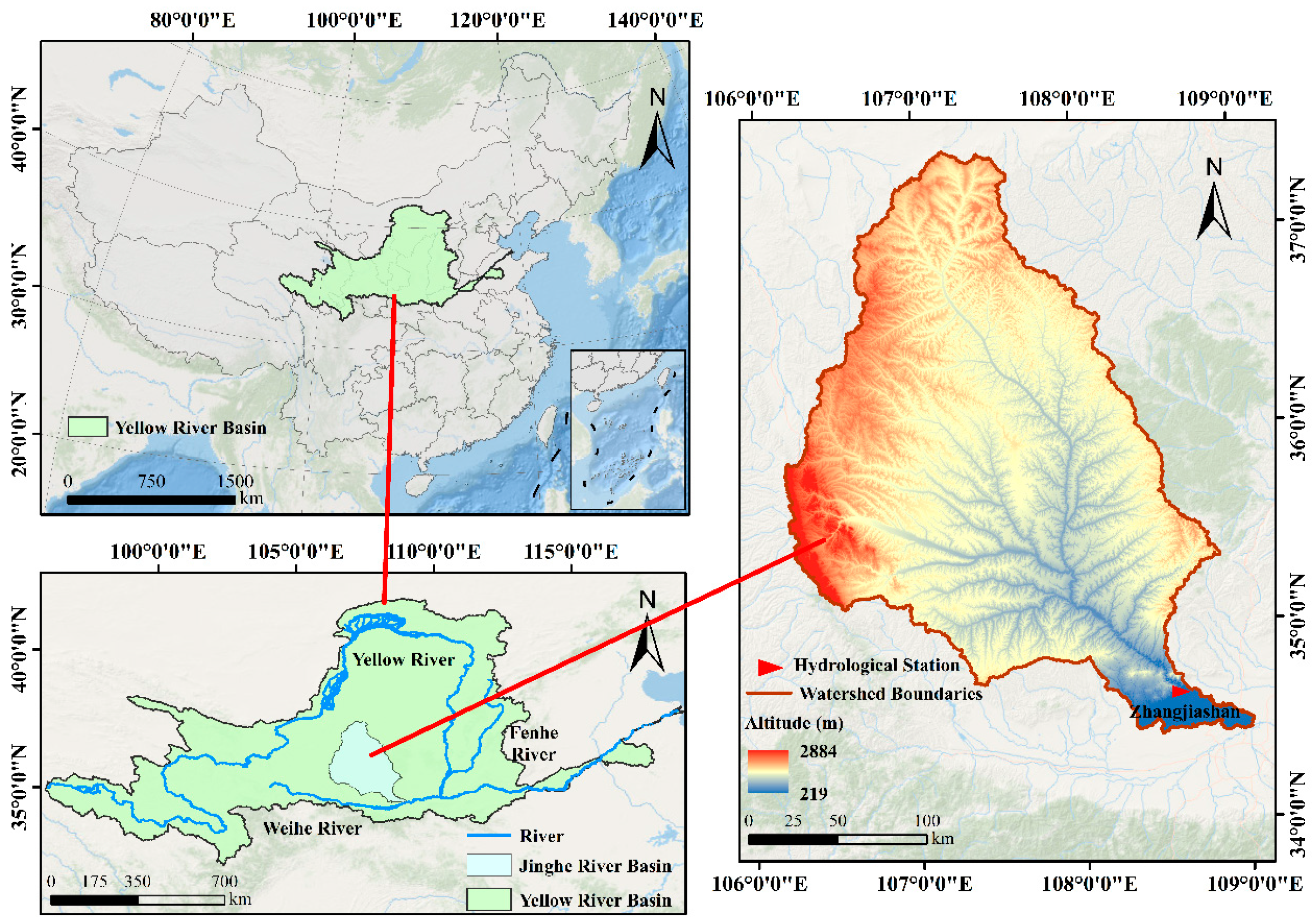
2.1. Study Area

Originating at the foothills of the Liupan Mountains, the JRB extends between 106°14′~108°42′ E and 34°46′~37°19′ N (Figure 1). The main river of the JRB extends approximately 455.1 km, and the basin covers an area of about 45,000 km². Flowing through Gansu, Shaanxi, and Ningxia provinces, it acts as a secondary tributary of the Yellow River. The terrain of the basin is intricate, characterized by higher elevations in the northwest and lower elevations in the southeast. The climate of the Jing River basin is temperate continental, featuring a mean annual temperature of about 10 °C and annual precipitation ranging from 290 to 560 mm. The precipitation changes obviously within the year, mostly concentrated in summer [38,40]. Farmland and grassland are the dominant land cover types in the JRB, making up over 85% of its total area [41]. The soil is primarily composed of calcaric cambisols, which are weak in wind and water erosion resistance and prone to soil erosion.

2.2. Data Source

The data sources for the SWAT and PLUS models are outlined in

Table 1. Data types and sources.

Model	Data Type	Data	Data Source
SWAT	Digital elevation data	DEM	Geospatial Data Cloud (https://www.gscloud.cn)
	Meteorological data	CMADS V1.1 Datasets (2008–2016)	The China Meteorological Assimilation Driving Datasets for the SWAT mode (https://cmads.org/)
	Hydrological data	Runoff data (2008–2016)	‘Hydrological Yearbook of the Yellow River Basin’
	Land use data	Land use data (2000, 2005, 2010, 2015, 2020)	Institute of Geographic Sciences and Natural Resources Research, Chinese Academy of Sciences (https://www.resdc.cn)
	Soil data	Chinese Soil Dataset (v1.1) Based on World Soil Database (HWSD)	The National Cryosphere Desert Data Center (http://www.ncdc.ac.cn)
PLUS	Land use data	Land use data (2010, 2015, 2020)	Institute of Geographic Sciences and Natural Resources Research, Chinese Academy of Sciences (https://www.resdc.cn)
	Socio-economic factor	Population (2020)	Resource and Environmental Science and Data Platform (https://www.resdc.cn/)
		GDP (2020)
	Accessibility factor	Distance from first level road (2020)	The National Catalogue Service for Geographic Information (https://www.webmap.cn/main.do?method=index (accessed on 24 July 2024))
		Distance from second level road (2020)
		Distance from third level road (2020)
		Distance from county government (2020)
		Distance from water area (2020)
	Natural geographic factor	Soil data	The National Cryosphere Desert Data Center (http://www.ncdc.ac.cn)
		Mean annual temperature (2020)	Resource and Environmental Science and Data Platform (https://www.resdc.cn/)
		Mean annual precipitation (2020)
		DEM	Geospatial Data Cloud (https://www.gscloud.cn)
		Slope	Generated from DEM

.

(1) SWAT 10.2 model data: With a spatial resolution of 30 m, the land use data (LUD) is categorized into 6 categories (farmland, forest land, grassland, water, construction land, and unused land) according to the classification index of the Resource and Environmental Science Data Center of the Chinese Academy of Sciences and the SWAT model land use classification standard. The soil dataset, possessing a spatial resolution of 1 km, was categorized into 20 distinct classes following the classification criteria specified by the SWAT model. The Soil, Plant, Atmosphere, and Water (SPAW) model was employed to compute essential soil parameters. Using DEM data with a spatial resolution of 30 m, sub-basins are defined, and river networks are extracted. This study employs hydrological data, consisting of monthly flow measurements from the Zhangjiashan hydrological station in the JRB, recorded over the period 2008 to 2016. Based on data availability, meteorological parameters such as precipitation, temperature, relative humidity, solar radiation, and wind speed were all sourced from the China Meteorological Assimilation Driving Datasets (CMADS) V1.1 dataset (2008–2016), which features a spatial resolution of 0.25° × 0.25°.

(2) PLUS 1.3.5 model data: Baseline inputs included LUD from 2010, 2015, and 2020. Following the approaches of Hu et al. [42] and Yu et al. [43], socio-economic data, distance factors, and climatic and environmental-related data were chosen as LUCC influencing factors. The population distribution in socio-economic factor affects land demand, while the Gross Domestic Product (GDP) reflects the impact of urban and industrial restructuring on land use. Distance factors, including proximity to transportation networks, administrative centers, and water resources, influenced socio-economic activities and land use patterns. Climatic and environmental data, including soil, temperature, precipitation, and slope, affected vegetation growth and the spatial allocation of land use categories. While the DEM-derived slope and aspect data had a resolution of 30 m, all other data were uniformly resampled to a standardized 30 m×30 m resolution to ensure consistency.

2.3. SWAT Model

In 1994, the US Department of Agriculture created the SWAT model. This model represents a semi-distributed hydrological model with strong physical mechanisms and is well-suited for long-term time series simulations [44]. It also takes into account meteorological and geomorphic factors to effectively simulate the effect of temporal variations in land use patterns, meteorological conditions, soil types, and other variables on the water cycle of the basin [45].

2.3.1. Sensitivity Analysis

Due to numerous parameters in the SWAT model, the SUFI-2 algorithm created by Abbaspour et al. is widely employed. This approach enables the determination of the model’s optimal parameters by conducting parameter sensitivity analysis and performing multiple iterations [46,47]. To enhance the model’s operational efficiency, this study selected 16 runoff-related parameters based on watershed characteristics. The SWAT-CUP 2019 software was employed to simulate runoff at the Zhangjiashan station across multiple land use scenarios, applying the SUFI-2 algorithm for sensitivity analysis, calibration, and validation.

2.3.2. Calibration and Validation

Considering the natural flow direction of rivers and the monitoring zones of hydrometric stations, the JRB was segmented into 120 sub-basins. The model combines the CMADS V1.1 dataset and the temporal series of observed runoff data, establishing warm-up (2008), calibration (2009–2011), and validation periods (2012–2016). With the 2010 LUD as the baseline and without altering the meteorology, soil, and HRU data, SWAT models were established for five LUCC scenarios in 2000, 2005, 2015, and 2020, and runoff simulations were conducted for each scenario. The model’s applicability was evaluated based on four metrics: the correlation coefficient (R²), Nash–Sutcliffe efficiency coefficient (NSE), percent bias (PBIAS), and the ratio of the root mean square error to the standard deviation (RSR). Generally, the model simulation results are considered reliable when R > 0.6, N > 0.5, RSR ≤ 0.7, and PBIAS falls within ±25% [48,49].

$$R^2={{\displaystyle \frac{\left[{\displaystyle {\sum }_{i=1}^{\mathrm{n}}\left(Q_{obs,i}-\stackrel{-}{Q_{obs}}\right)\left(Q_{sim,i}-\stackrel{-}{Q_{sim}}\right)}\right]}{{\displaystyle {\sum }_{i=1}^{\mathrm{n}}{\left(Q_{obs,i}-\stackrel{-}{Q_{obs}}\right)}^2{\displaystyle {\sum }_{i=1}^n{\left(Q_{sim,i}-\stackrel{-}{Q_{sim}}\right)}^2}}}}}^2$$

(1)

$$NSE=1-{{\displaystyle \frac{{\displaystyle {\sum }_{i=1}^{\mathrm{n}}\left(Q_{obs,i}-Q_{sim,i}\right)}}{{\displaystyle {\sum }_{i=1}^n{\left(Q_{obs,i}-\stackrel{-}{Q_{obs}}\right)}^2}}}}^2$$

(2)

$$PBIAS={\displaystyle \frac{{\displaystyle \sum _{i=1}^n(}{Q}_{obs,i}-Q_{sim,i})\ast 100}{{\displaystyle \sum _{i=1}^n{Q}_{obs,i}}}}$$

(3)

$$\mathrm{R}\mathrm{S}\mathrm{R}={\displaystyle \frac{\sqrt{{\displaystyle \sum _{\mathrm{i}=1}^{\mathrm{n}}{({\mathrm{Q}}_{\mathrm{o}\mathrm{b}\mathrm{s},\mathrm{i}}-{\mathrm{Q}}_{\mathrm{s}\mathrm{i}\mathrm{m},\mathrm{i}})}^2}}}{\sqrt{{\displaystyle \sum _{\mathrm{i}=1}^{\mathrm{n}}{({\mathrm{Q}}_{\mathrm{o}\mathrm{b}\mathrm{s},\mathrm{i}}-\stackrel{-}{{\mathrm{Q}}_{\mathrm{o}\mathrm{b}\mathrm{s}}})}^2}}}}$$

(4)

where $n$ represents the number of observed values; $Q_{obs,i}$ denotes the measured runoff (m³/s); $\stackrel{-}{Q_{obs}}$ is the mean measured runoff (m³/s); $Q_{sim,i}$ is the simulated runoff (m³/s); $\stackrel{-}{Q_{sim}}$ is the mean simulated runoff (m³/s).

2.4. Land Use Dynamic Index

The land use dynamic degree is a key quantitative indicator for assessing the rate of land type changes in a given region. The single land use dynamics index (K) is designed to assess changes in specific land types. The comprehensive land use dynamic index (LC) characterizes the intensity and features of LUCC across the entire study area [50]. The following formulas are provided:

$$K={\displaystyle \frac{U_b-U_a}{U_a}}\times {\displaystyle \frac{1}{T}}\times 100\%$$

(5)

$$LC={\displaystyle \frac{{\displaystyle \sum _{i=1}^n\mathsf{\Delta }{S}_{i-j}}}{{\displaystyle \sum _{i=1}^n{S}_i}}}\times {\displaystyle \frac{1}{T}}\times 100\%$$

(6)

where $U_a$ and $U_b$ represent the area of a given LUT at the beginning and end of the study, respectively; $T$ refers to the study period (usually set as a year); $S_i$ represents the area of LUT $i$ during the research period; $\mathsf{\Delta }{S}_{i-j}$ denotes the transition area of LUT from class $i$ to class $j$ during the research period.

2.5. PLUS Model

The PLUS model combines the Land Expansion Analysis Strategy (LEAS) and the Cellular Automata model with Multi-type Random Patch Seeds (CARS), enabling precise simulations of land use patch scale changes across various years and environmental conditions [51].

2.5.1. Distribution Probability of Land Use Types

(1) Using the Land Expansion Analysis Strategy (LEAS) within the PLUS model, the conversion rules of LUT in the JRB are explored, and the development probabilities for each type are obtained. The mathematical formula is as follows [52]:

$$P_{i,k}^t(x)={\displaystyle \frac{{\displaystyle \sum _{\mathrm{n}=1}^M[I(h_n(x)=d)}]}{M}}$$

(7)

where $x$ is the vector representing the driving factor; $P_{i,k}^t(x)$ indicates the probability of LUT growth in the cell $i$; when $d$ is 1, non $k$-type land is converted to $k$-type, and when $d$ is 0, the conversion of $k$-type land is not included; $M$ stands for the total number of decision trees; $I()$ indicates the exponential function of the decision tree; $h_n(x)$ indicates the indicator function for the $x$th decision tree combination of vector $n$.

(2) Using the CARS module, constraints are applied to the development probabilities of various land types, and their overall probabilities are calculated to model the land use distribution pattern. The formula is as follows [52]:

$$O{P}_{i,k}^{d=1,t}=P_{i,k}^d{\mathsf{\Omega }}_{i,k}^t{D}_k^t$$

(8)

where $O{P}_{i,k}^{d=1,t}$ represents the comprehensive probability of the $i$th cell transitioning to land type $k$ at $t$; $P_{i,k}^d$ refers to the probability of land type $k$ expanding within $i$ cells; ${\mathsf{\Omega }}_{i,k}^t$ is the domain effect of cell $i$; $D_k^t$ refers to the impact of future demand on the type of $k$ land.

2.5.2. Multiple Scenario Settings

Based on the development of LUCC in the JRB from 2000 to 2020, “Regulations on Reforesting Cultivated Land”, “Guiding Opinions on Promoting the High-Quality Development of Water and Soil Conservation in the Yellow River Basin”, and “Overall Land Use Plan of Shaanxi Province (2021–2035)”, the following three scenarios are established in this study.

(1) Inertial Development Scenario (S1): Based on current evolution law, and without any imposed influences, the Markov Chain method is employed to forecast the various LUT under the natural scenario for the year 2030.

(2) Farmland Protection Scenario (S2): In this scenario setting, the transformation rate from grassland and forest to construction land is cut by 20%, whereas the likelihood of farmland being converted into construction land declines by 60% [53].

(3) Ecological Protection Scenario (S3): The likelihood of grassland and forested areas transitioning into urban development zones is diminished by 20%. Concurrently, the transformation probability of aquatic ecosystems into built-up areas experiences a more substantial reduction of 30% [54].

2.5.3. Neighborhood Weights

The neighborhood weights, quantified on a scale from 0 to 1, reflect the relative expansion potential across distinct land use categories. A higher value indicates increased difficulty in converting that land type to others, implying stronger expansion capability. The field weights are determined based on the dimensionless value of $\mathsf{\Delta }TA$, calculated using the following formula [55]:

$$w_i={\displaystyle \frac{\mathsf{\Delta }TAi-\mathsf{\Delta }T{A}_{\min }}{\mathsf{\Delta }TA{i}_{\max }-\mathsf{\Delta }T{A}_{\min }}}$$

(9)

where $\mathsf{\Delta }TAi$ is the variation in the expansion area of different land types; $\mathsf{\Delta }T{A}_{\min }$ corresponds to the minimum observed change in the expansion area across regions; $\mathsf{\Delta }TA{i}_{\max }$ refers to the maximum expansion area change in various regions. Since the conversion probability of different categories cannot be zero in practical situations, the term with a median domain weight of 0 is reset to 0.1 to make it more relevant to the actual situation. The results of setting domain weights are presented in

Table 2. The parameter of neighborhood weight.

Land Use Type	Farmland	Forest Land	Grassland	Water	Construction Land	Unused Land
S1	0.1	0.46	1	0.53	0.61	0.54
S2	0.1	0.44	1	0.52	0.59	0.51
S3	0.1	0.32	1	0.42	0.27	0.41

.

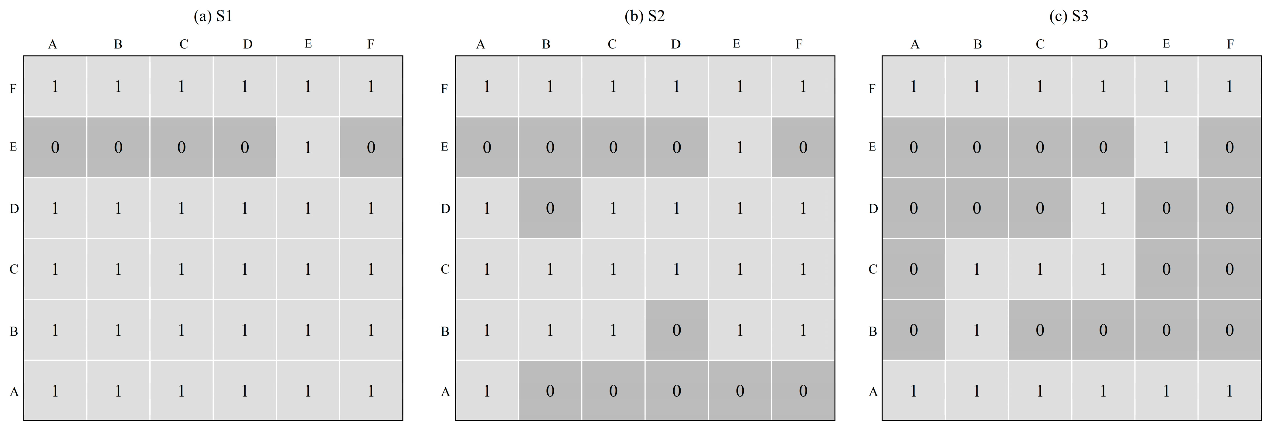
2.5.4. Conversion Cost Matrix

The transformation probability matrix establishes the probabilistic framework governing inter-conversion among diverse land use classifications. Specifically, a matrix value of 1 indicates that a given land type is allowed to transition into another, whereas a value of 0 denotes that such a conversion is prohibited (Figure 2).

2.5.5. Model Accuracy Verification

The Kappa coefficient varies between 0 and 1, where higher values reflect greater simulation accuracy. A detailed assessment of simulation accuracy is provided in

Table 3. Kappa coefficient classification evaluation criteria.

Kappa Coefficient	<0.00	0.00~0.20	0.21~0.40	0.41~0.60	0.61~0.80	0.81~1.00
Level	Very poor	Slight	Fair	Moderate	Substantial	Almost Perfect

[56].

$$K\mathrm{appa}={\displaystyle \frac{P_0-P_c}{P_p-P_c}}$$

(10)

where $P_0$ represents the simulated proportion of the correct grid; $P_p$ denotes the proportion for accurate simulation; $P_c$ signifies the simulated correct ratio under random state.

3. Result Analysis

3.1. Calibration and Validation of the SWAT Model

The SUFI-2 algorithm integrated into the SWAT-CUP program was utilized to assess parameter sensitivity and perform calibration. The computational procedure commenced with a comprehensive global sensitivity evaluation, executing 3000 simulation runs on the initial parameter configuration. Applying the established sensitivity evaluation metrics (wherein parameters demonstrating p-values approaching zero or exhibiting elevated absolute t-stat values are considered more influential) [57], the analysis yielded 16 key parameters demonstrating significant sensitivity to hydrological processes (refer to Appendix A for more details). Subsequently, through an additional 2000 iterations of calibration, parameters with low sensitivity and significance were excluded based on the t-stat and p-value results. Ultimately, 11 parameters with significant sensitivity were selected. (

Table 4. Ranking of parameter sensitivity.

Rank	Parameter	Description	Optimal Value	Parameter Range
1	V__CH_K2.rte	Effective hydraulic conductivity in main channel alluvium	0.186	0~150
2	V__CH_N2.rte	Manning’s n value for main channel	0.214	0~0.3
3	R__SOL_AWC(..).sol	Soil available water storage capacity	0.415	−0.2~1
4	V__CN2.mgt	SCS runoff curve number	55.418	35~98
5	R__HRU_SLP.hru	Average slope steepness	0.288	0~0.6
6	V__TLAPS.sub	Temperature lapse rate	−7.188	−10~10
7	V__GW_DELAY.gw	Groundwater delay time	390.114	0~500
8	V__EPCO.hru	Plant uptake compensation factor	0.891	0~1
9	R__SOL_ALB(..).sol	Surface reflectance	−0.015	0.25~0.25
10	V__BIOMIX.mgt	Biological mixing efficiency	0.663	0~1
11	R__SOL_Z(..).sol	Soil depth	0.385	−0.5~0.5

Note: r represents the parameter value multiplied by (1 + calibration value), while v refers to the parameter value replaced by the calibration value.

). The effective hydraulic conductivity in the main channel alluvium (CH_K2) is the most sensitive parameter, followed by Manning’s n value for the main channel (CH_N2). The soil available water storage capacity (SOL_AWC) and SCS runoff curve number (CN2) are sensitive to the simulation of runoff from the JRB.

During the calibration (2009–2011) and validation (2012–2016) process in the basin, the selected parameters were continuously adjusted, ultimately resulting in the determination of the value ranges and optimal values. The optimal parameter values were entered into the SWAT model. The results show that the calibration period with R² = 0.91, NSE = 0.84, PBIADS = 10% and RSR = 0.44, while the validation period resulted in R² = 0.90, NSE =0.85 PBIADS = 4.4% and RSR = 0.39. This means that the SWAT model demonstrates strong applicability for simulating runoff in the JRB.

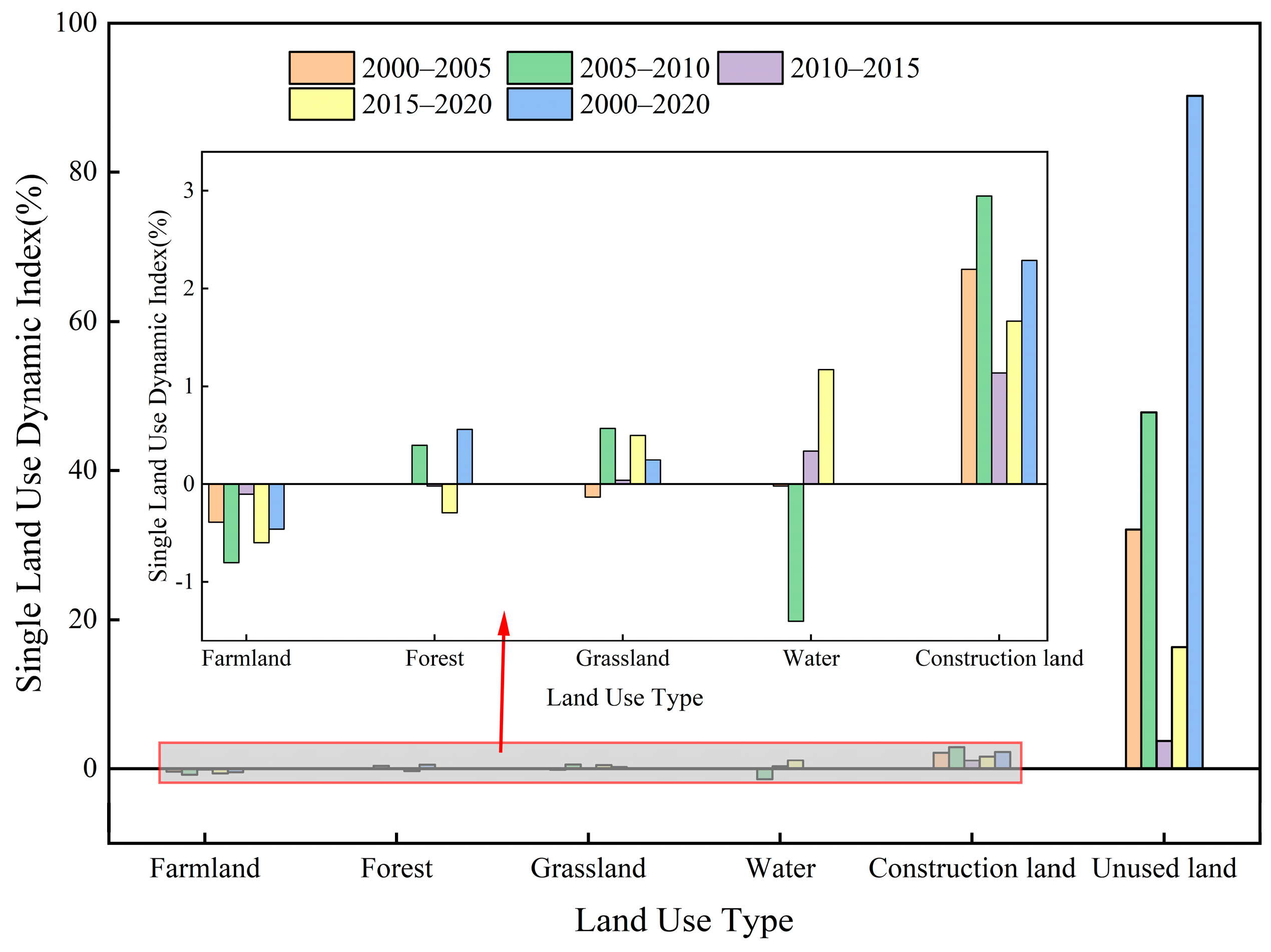
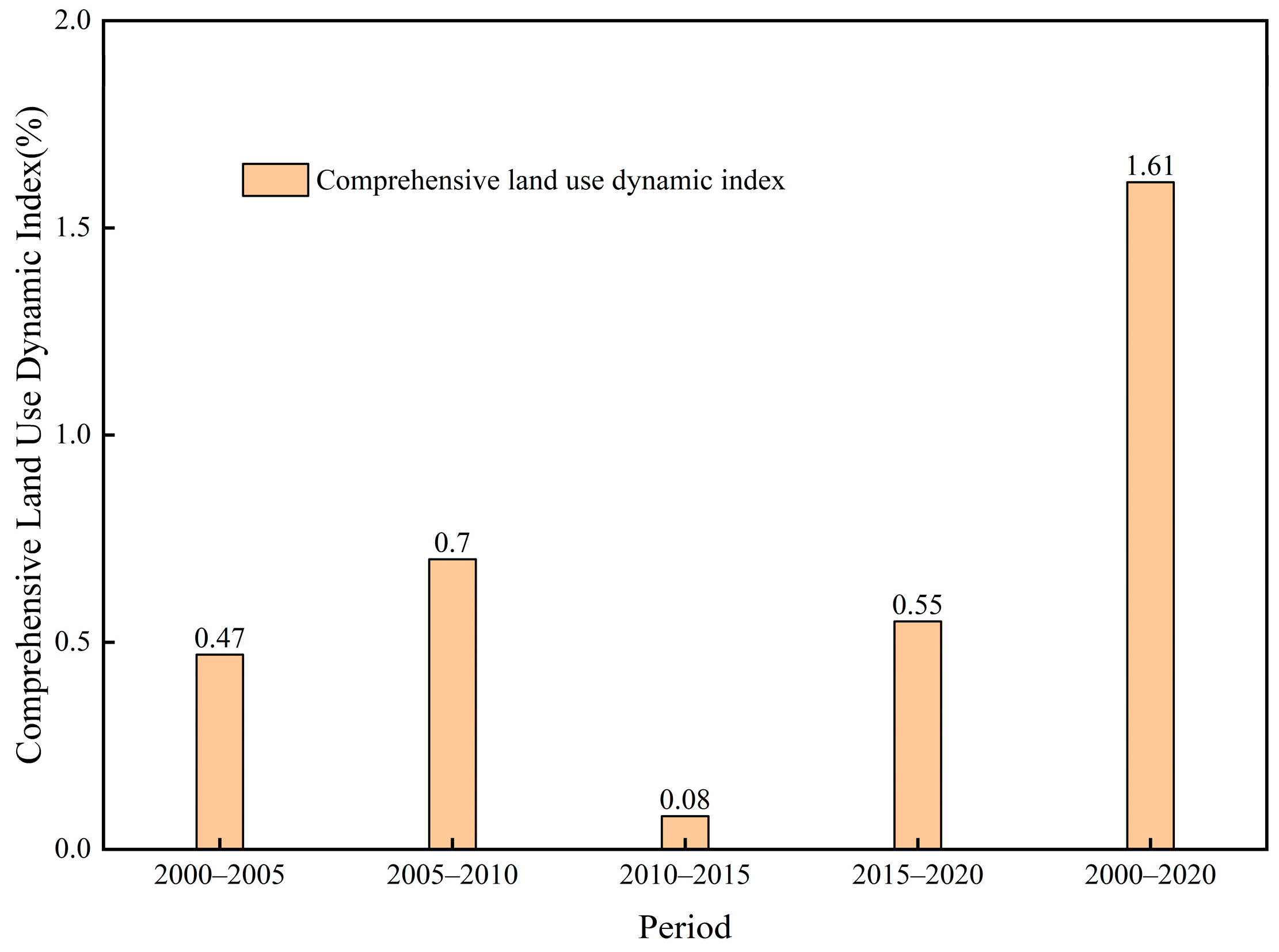
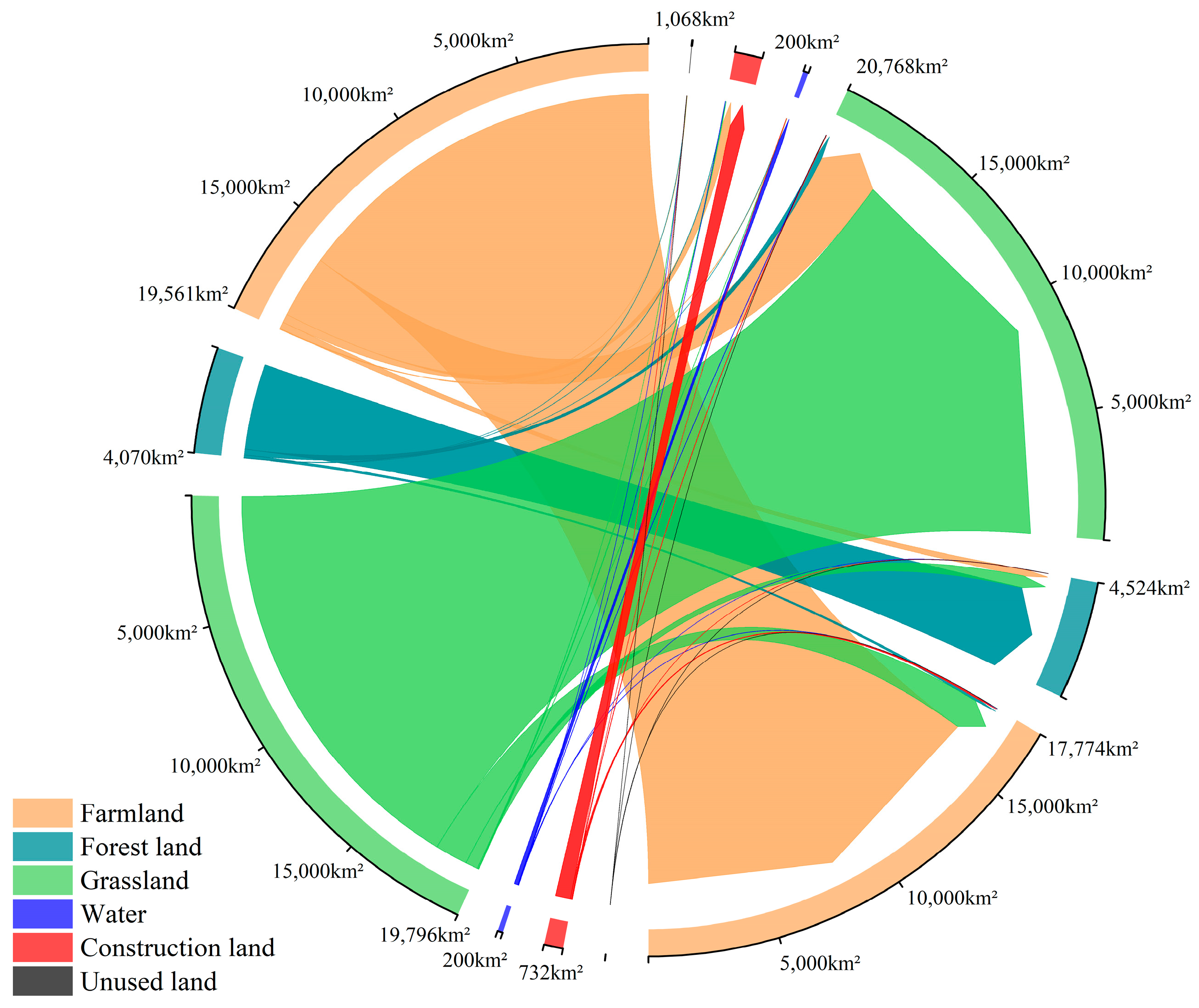
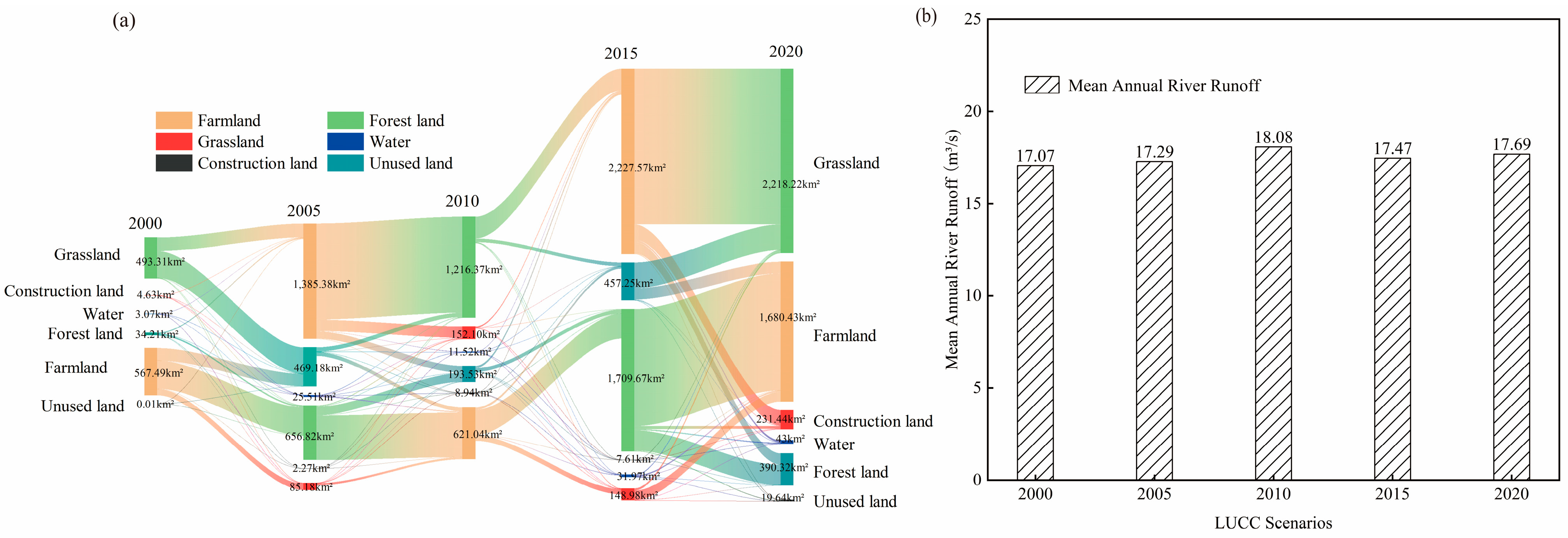
3.2. Features of Land Use/Cover Change

From Figure 3, grassland dominated the JRB, representing around 45% of the total area from 2000 to 2020, with a net growth of 972.3 km² over the period. Secondly, the farmland represents around 42% of the total area, but its overall area has decreased by 1787.8 km² over the same period. The forest land showed a fluctuating growth of 454.6 km². Meanwhile, construction land and unused land increased by 335.8 km² and 25.4 km², respectively, with unused land representing the least share of the total area.

According to Figure 4, the change rate of LUT in the JRB from 2000 to 2020 was in descending order: unused land (increased by 90.28%), construction land (grew by 2.29%), forest land (grew by 0.56%), farmland (declined by 0.46%), grassland (grew by 0.25%), and water (small change of about 0%). The LUD across the five periods was divided into four phases, and it was found that unused land, construction land, water, farmland and grassland changed obviously from 2005 to 2010. Forest land (increased by 2.14%) showed an obvious growth rate from 2000 to 2005. This trend may be associated with aspects like economic development, conversion of farmland back into forests, and ecological policies [58]. Compared to other LUTs, the increased rate of unused land use is obvious, which may be affected by natural disasters, changes in agricultural policies, decline in market demand and environmental degradation [59].

As illustrated in Figure 5, the dynamic index of comprehensive land use in 2000–2020 was 1.61%. Specifically, the comprehensive land use dynamic index across the four study periods, with calculated values of 0.47%, 0.70%, 0.08% and 0.55%, respectively. The comprehensive land use dynamic index from 2005 to 2010 was obviously higher than that of other periods, because of the increase in grassland and construction land, which grew by 559.5 km² and 119.8 km², respectively. Additionally, the lowest comprehensive land use dynamic index between 2010 and 2015 resulted from the relatively small changes in different LUTs during this time. The trends in LUT changes differed across various periods. From 2000 to 2005 and 2005 to 2010, farmland and water areas declined, whereas forest land and construction land expanded. From 2000 to 2005, the grassland area declined, but it increased from 2005 to 2010. In addition, from 2010 to 2015 and from 2015 to 2020, farmland and forest land areas declined, whereas grassland, water, construction land, and unused land areas expanded.

As shown in Figure 6, the transfer areas of water and unused land were minimal, with the majority of the conversions occurring through mutual conversions between farmland, grassland, and forest land. Specifically, most farmland was transferred out, a total of 3400 km ², mainly converted into construction land and grassland. The grassland received the largest amount of transferred land (total area of 2982.4 km²), with 2702 km² primarily transferred from farmland. Farmland and forest land areas primarily originated from grassland, with an inward transfer of 1612 km² and 838 km², respectively. Construction land and unused land areas have expanded, mainly converted from farmland. By comparison, the transfer area of construction land, both inward and outward, is relatively limited.

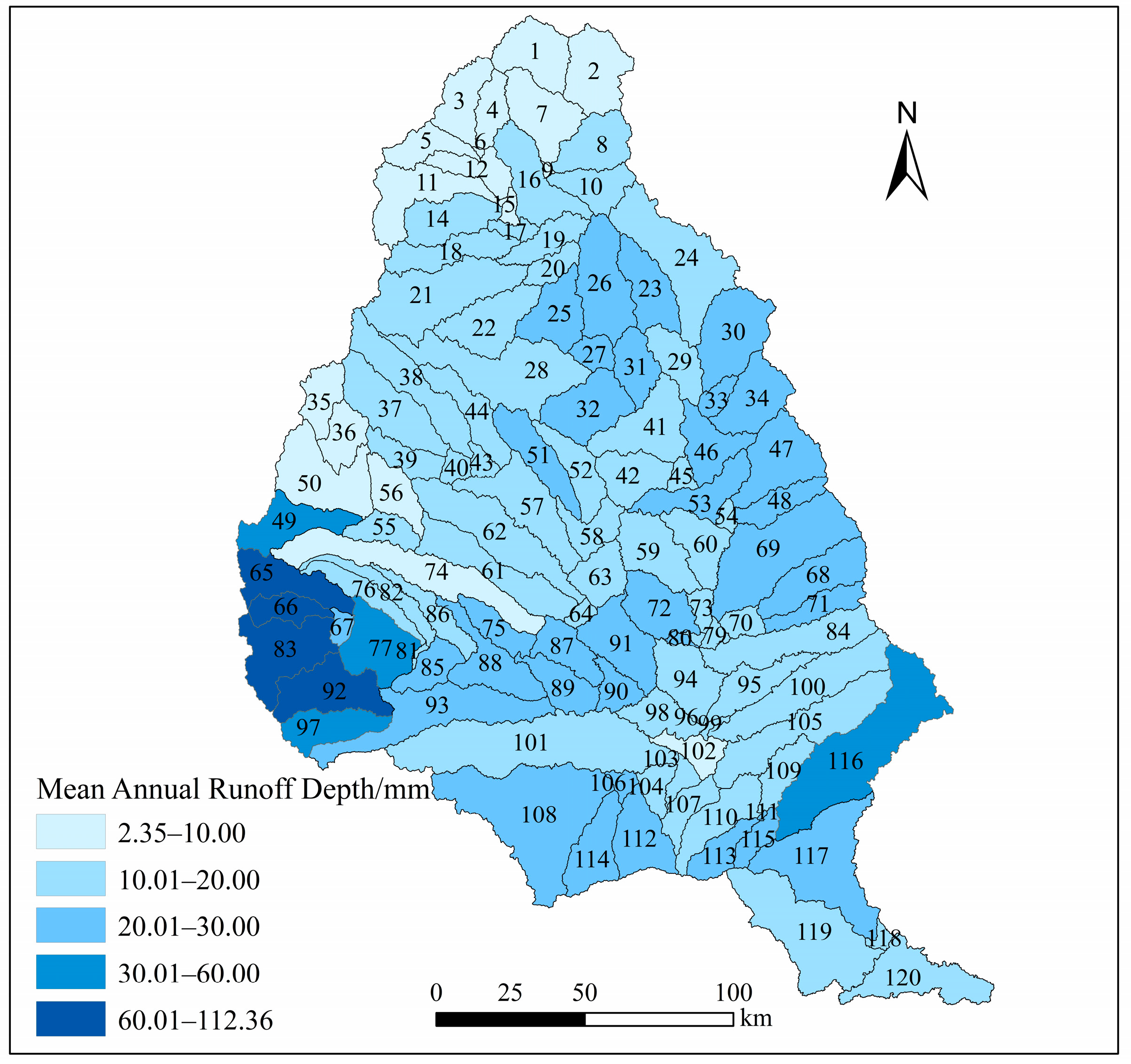
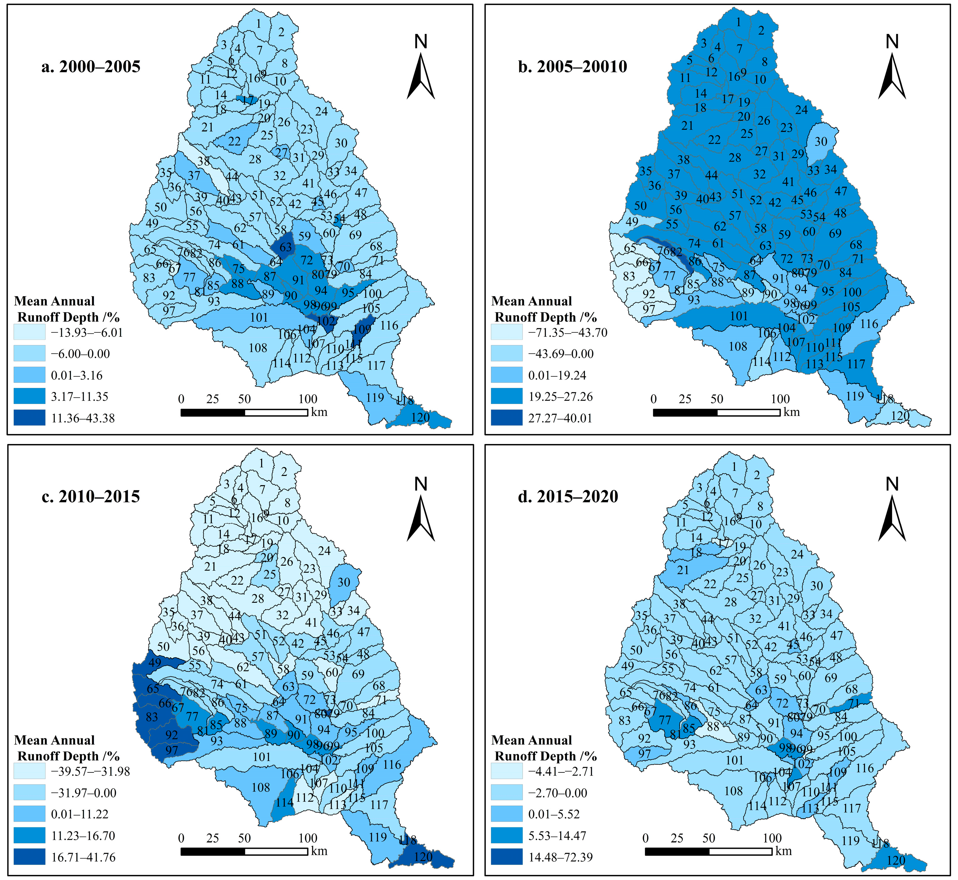
3.3. Impact of Land Use/Cover Change on Runoff

For a quantitative analysis of the effects of different land use scenarios on runoff, the SWAT model was calibrated and verified using 2010 LUD, and the optimal parameters were selected for model adjustment. Subsequently, LUD from 2000, 2005, 2015, and 2020 were sequentially imported into the model while keeping the meteorological, soil, slope data, and HRU threshold settings unchanged, to obtain simulated runoff values for the five land use scenarios. As illustrated in Figure 7, the trend of measured runoff and simulated runoff changes are quite similar. The measured and simulated peak flood values show good consistency, and the wet and dry seasons align closely in timing.

From a temporal perspective (Figure 8 and

Table 5. Changes in land use/cover (km²).

Land Use Type	2000–2005	2005–2010	2010–2015	2015–2020
Farmland	−386.1	−764.3	−90.3	−547.1
Forest land	435.02	90.24	−3.76	−66.92
Grassland	−131.2	559.5	35.5	508.5
Water	−0.21	−13.99	3.19	11.03
Construction land	80.55	119.81	52.96	82.46
Unused land	2.25	8.75	2.34	12.03

), the annual average runoff simulated using LUD from 2000 to 2020 exhibits a dynamic upward trend. Comparing the 2000 and 2005 land use scenarios, the annual average runoff increased by 0.22 m³/s. During this period, farmland and grassland areas declined by 386.1 km² and 131.2 km², respectively, while construction land increased by 80.56 km². In terms of land transfer, farmland and grassland primarily shifted to forest land and construction land. Between the 2005 and 2010 land use scenarios, the increase in annual average runoff was relatively more obvious, rising by 0.79 m³/s. Farmland area decreased by 764.3 km², while forest land, grassland, construction land, and unused land expanded by 90.24 km², 559.5 km², 119.8 km², and 8.75 km², respectively. During this period, farmland saw the greatest transfer, predominantly to grassland, while the transfer of construction land increased, mainly from farmland. Under the 2000–2010 land use scenarios, the trend of increasing annual average runoff continued. Although grassland and forest land areas increased, the rapid urbanization led to greater reductions in farmland and expansions in unused land and construction land, increasing impervious surfaces within the watershed, thereby augmenting runoff. Comparing the 2010 and 2015 land use scenarios, the annual average runoff decreased. The reduction in various land use transfers was characterized mainly by farmland transitioning into grassland, with an area of 300.5 km², indicating that the interception function of grassland contributed to the runoff reduction under this scenario. In contrast, between 2010 and 2015, the annual average runoff increased. Farmland and forest land areas declined by 547.1 km² and 66.92 km², respectively, whereas grassland, construction land, unused land, and water areas expanded by 508.5 km², 82.46 km², 12.3 km², and 11.03 km², respectively. During this period, farmland predominantly transitioned into grassland, with some also converting to construction land, while notable exchanges occurred between forest land and grassland. Despite the grassland area increase, ongoing urbanization led to continuous reductions in farmland and forest land, replaced by construction land. This expansion of impervious surfaces diminished the infiltration efficiency and capacity of surface runoff, directly resulting in higher surface runoff.

From a spatial perspective, there are obvious spatial differences in mean annual runoff depths (MARD) across sub-basin units (Figure 9). The mean runoff depth in the upstream regions is lower than that in the downstream regions. The runoff depth distribution is relatively uniform in the East, whereas the MARD varies significantly across the Western sub-basins. The MARD of sub-basins 65, 66 and 83 in the West is obviously higher than that of other sub-basins.

According to Figure 10, the MARD in the middle and lower reaches areas of the JRB under the 2005 LUU scenario increased by 0% to 43.38% compared to the 2000 LUCC. The growth rate in certain areas of the middle reaches is relatively large, ranging from 3.17% to 43.38%, due to the increase in runoff resulting from the decline in farmland and the growth in construction land. Compared with the 2005 LUCC, the MARD across the majority of the basin rose in the LUCC scenario of 2010, except in Western regions. Notably, the MARD in the midstream and upstream reaches increased by a range of 19.25% to 40.01%. This is due to the increased conversion of farmland into construction land, which has increased impervious surfaces and facilitated the rise in runoff consequently. Compared with the LUCC scenario in 2010, the 2015 LUCC scenario shows an uptrend in MARD in the sub-basins near the Liupan Mountains and at the basin outlet. In contrast, most other regions exhibited a downtrend, with reductions ranging from 0% to 39.57%. This decline results from the considerable transformation of farmland into grassland and grassland into forest, leasing to enhancing plant interception and capabilities for conserving soil and water. Furthermore, in comparison to the 2015 LUCC scenario, the decline of farmland and forest land in most areas of the watershed contributed to a rise in MARD in the 2020 LUCC scenario, with a rise ranging from 0% to 72.39%.

To further explore the influence of LUCC on runoff, this study selected the sub-basins with the largest increase in four periods for analysis: sub-basin 102 (Figure 10a), sub-basin 82 (Figure 10b), sub-basin 92 (Figure 10c), and sub-basin 96 (Figure 10d). As depicted in

Table 6. Land area of various types of sub-basins (km²).

Land Use Type	Sub-Basin 102		Sub-Basin 82		Sub-Basin 92		Sub-Basin 96
	2000	2005	2005	2010	2010	2015	2015	2020
Farmland	125.61	124.14	114.19	113.85	200.84	198.99	0.30	0.24
Forest land	5.79	5.79	3.11	4.29	64.92	64.80	-	-
Grassland	46.66	47.04	92.76	91.88	249.29	249.49	0.04	0.02
Water	6.08	6.09	0.07	0.06	0.45	0.59	-	-
Construction land	9.04	10.11	4.35	4.40	10.74	11.66	-	0.08
Unused land	-	-	-	-	0.16	0.87	-	-

, the increase in MARD in sub-basin 102 is attributed to the decrease in farmland area (1.47 km²) and the growth in constructed land (1.07 km²). In sub-basin 82, the rise in MARD is noteworthy. Although there was an increase in forestland area (1.18 km²), the reductions in farmland (0.34 km²), grassland (0.87 km²), and water (0.0054 km²), along with the increase in constructed land (0.04 km²), exceeded the gains in forest land area. For sub-basin 92, the increase in MARD is influenced by the reduction in farmland (1.85 km²) and forested area (0.12 km²), as well as the expansion of constructed land (0.95 km²) and water (0.14 km²). In sub-basin 96, the rise in MARD is attributed to the decline in farmland (0.5 km²) and grassland area (0.03 km²), combined with the growth in constructed land area (0.8 km²). Overall, the decrease in grassland, farmland, and forested areas contributes to higher runoff, while the growth of constructed land similarly increased runoff.

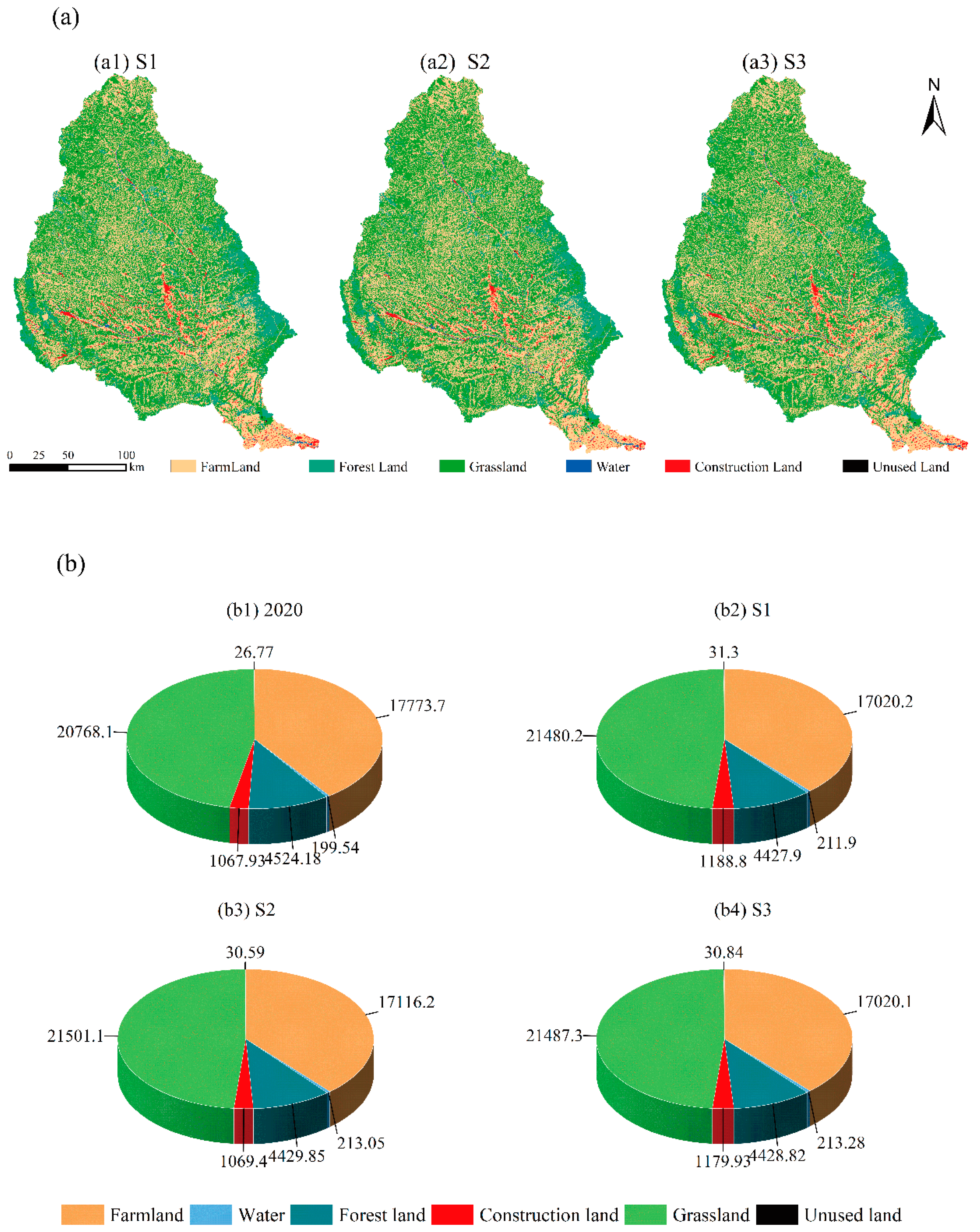
3.4. Future Land Use/Cover Scenarios and Runoff Projections

This study is based on LUD from 2010 and 2015 to forecast the land situation in 2020. The prediction results were compared to the real 2020 LUCC data using the Kappa coefficient. The Kappa coefficient is 0.810, the FoM is 0.11 and the overall accuracy is 0.884, the high accuracy demonstrates that the PLUS model performs effectively in simulating land use in the JRB. Using the 2020 LUD as the starting year, three scenarios were established for the JRB in 2030. As shown in Figure 11a, the distribution of LUT in the JRB remained largely unchanged under the three LUCC scenarios in 2030. In addition, farmland and grassland continued to be the primary LUT, with their combined area exceeding 86% of the total basin area. Compared to the 2020 LUD (Figure 11b), the S1 scenario has the largest decline in forest land (96.3 km²) and growth in constructed land (121 km²). In the S2 scenario, influenced by Cropland Protection Policies, the reduction in farmland (657.5 km²) and the increase in constructed land (1.47 km²) are the smallest. The S3 scenario is affected by ecological protection policies, with the largest reduction in farmland area (753.6 km²) and an increase in water and grassland areas.

The SWAT model received LUD for the three 2030 scenarios projected using the PLUS model. The settings for meteorological data, soil, slope, and HRU thresholds were kept constant throughout the process, and the runoff values were subsequently simulated. As shown in Figure 12a, the mean annual runoff of the three scenarios showed an uptrend compared to 2020. Specifically, the mean annual runoff in scenarios S1 and S2 increased by 8.31% and 1.02%, respectively, compared to 2020. In the S2 scenario, the change in mean annual runoff was minimal, with a growth rate of only 0.06%. This change may be related to a decrease in farmland and forest land, along with the expansion of construction land. As illustrated in Figure 12b, the MARD in the JRB exhibits a relatively similar distribution in the 2020 LUCC scenario and the three scenarios for 2030. The downstream runoff depth is higher than the upstream, with a relatively uniform distribution in the central and eastern regions. The sub-basins 65, 66, and 83 in the west still exhibit higher runoff depths. Specifically, under the S1 scenario, the MARD increased compared to 2020 in the western sub-basins 67 and 55, the eastern sub-basins 47, 48, and 68, as well as the midstream sub-basins 72 and 91, and the downstream sub-basin 102. Under the S2 scenario, the MARD exhibits relatively slight changes in each sub-basin. Under the S3 scenario, sub-basins 72 and 91 in the middle reaches exhibit a rise in MARD. It is essential to continue monitoring these areas in the future and reinforcing efforts in soil and water conservation remains crucial.

4. Discussion

The distribution and variation of different LUTs at the watershed scale have an impact on surface runoff, groundwater recharge, and evapotranspiration. The SWAT model is employed in this study to quantify and simulate how land use changes affect hydrological processes, thus uncovering the dynamic variations in runoff characteristics under various land use scenarios. The findings suggest that the SWAT model demonstrates good applicability in the JRB. In terms of parameter sensitivity, four parameters are identified as the most critical for runoff simulation in the JRB. The CH_K2 parameter primarily controls the transmission losses of surface runoff when the sub-basins contribute to flow to the main river channel. The smaller the losses in the tributaries, the greater the runoff volume on the main channel [60]. In conditions of substantial surface runoff and a dense river network, the parameter CH_N2 has a more pronounced effect on the runoff generation [61]. The Jing River features a relatively dense river network, which contributes to the strong sensitivity of this parameter. Meanwhile, the parameter SOL_AWC reflects the capacity of soil to retain water, with larger parameter values indicating stronger soil water storage capacity and smaller runoff [62]. The parameter CN2 directly affects surface runoff and exhibits strong sensitivity across various basins. Its value is influenced by various factors, including land use practices and agricultural management measures [62,63]. Going forward, it will be important to focus on land use patterns, soil characteristics, and other factors to optimize and manage and optimize water resources in the JRB. Although the SWAT model demonstrated a good fit in this study, its practical application may still involve certain risks. For instance, it may underestimate the uncertainty in extreme event predictions, potentially compromising the reliability of management decisions. To enhance the model’s robustness, future research could refine parameter ranges, incorporate additional observational data, or employ alternative uncertainty analysis methods.

The runoff characteristics were simulated and compared using the SWAT + PLUS model under five land use scenarios and three future LUCC multi-scenarios. This study found that there was an obvious shift from farmland to forest land, grassland, and construction land in the JRB between 2000 and 2020. Similar results were reported by Yang Tao et al. in their study of the Weihe River Basin [64]. It reflects the impacts of urbanization, industrialization, the conversion of farmland back to forest policies, as well as ecological restoration and conservation strategies. Additionally, the reduction in farmland and forest land and the expansion of construction land promotes runoff, while grassland plays a suppressive role in runoff. These research results are consistent with the findings of Shi et al. [65] and Shrestha et al. [66]. This is because the conversion of farmland to construction land raises impervious surfaces, decreases infiltration capacity and leads to greater surface runoff. As grassland and woodland shrink, plant transpiration decreases, reducing evaporation. Moreover, the soil structure may be compromised, diminishing its ability to retain water and prevent erosion, ultimately leading to reduced runoff.

Using the PLUS model to forecast the three land use scenarios for 2030 revealed an increasing trend in runoff within the JRB. This finding is comparable to the predictions by Liu et al. [39] on how LUCC (2025, 2035, 2045) would influence runoff in the JRB. However, Liu et al. [39] did not consider the influence of land use policies in their predictions and only analyzed a single scenario. In contrast, this study comprehensively considers the dynamic nature of land policies and analyzes three distinct scenarios. Specifically, this study predicts that the average annual runoff under the S1 and S3 scenarios will increase compared to 2020. The primary reason is the decline in farmland and forest land, along with the expansion of construction land, which has promoted runoff. This finding aligns with previous studies indicating that decreased farmland and forest land, coupled with increased construction land, contribute to higher runoff [67,68]. In the S1 scenario, land use changes are typically driven by traditional development models, emphasizing economic growth and urbanization, potentially causing overexploitation and unequal distribution of water resources. Future efforts should focus on strengthening water resource management and environmental protection measures. In the S3 scenario, this approach helps to restore hydrological connectivity, allowing water flow to self-regulate within the natural environment. It enhances water retention and infiltration, thereby mitigating soil erosion and water loss. In the S2 scenario, the mean annual runoff shows little change compared to 2020. This is because the reductions in farmland and forest land, along with the rise in construction land, are roughly equal to the expansion of grassland and water. The S2 scenario emphasizes maintaining cropland areas, which generally have high water resource demands for agricultural use. To mitigate runoff and enhance water retention, vegetation strips can be planted between croplands, slowing runoff and increasing water interception. Additionally, adopting multi-layered or mixed cropping systems can improve vegetation cover and root distribution, thereby enhancing the water retention capacity of soil. Additionally, the sub-basins near the western Liupan Mountains exhibit higher runoff depth. This is partly due to the unique terrain (mountains and hills) and climate (warm temperate semi-humid) in the Liupan Mountains, which are conducive to the concentration and discharge of precipitation. Another contributing factor is the presence of karst water, which supplements the runoff in these areas [69]. Compared with 2020, the runoff depth of some sub-basins in the three land use scenarios in 2030 has obviously increased, which may be due to the growth in construction land and the decline in grassland and forest land areas. In the future, the government should plan and develop the land resources reasonably and also pay attention to preventing areas with high runoff depth and worsening soil erosion in the JRB.

Using the SWAT model and PLUS model, this study examines the spatio-temporal patterns of runoff changes under LUCC. However, there are still some shortcomings. Firstly, only LUD was modified while the meteorological, soil, and HRU data remained constant during the SWAT model simulation. Runoff variations are affected by factors such as climate, other human activities, slope, and soil characteristics, which will be the focus of the next research step. LUCC impacts runoff generation and distribution by altering surface characteristics and hydrological processes. Changes in precipitation patterns and a rise in extreme weather events may further intensify or alleviate the impact of LUCC on runoff. This interaction could complicate watershed water resource management and disaster risk reduction strategies. Therefore, it is crucial to comprehensively consider the hydrological response under the combined influence of LUCC and climate change when formulating effective watershed management and adaptation strategies. Secondly, this study combined CMADS and SWAT models to explore the effects of LUCC on the runoff in the JRB. The SWAT model powered by CMADS data sets can simulate runoff well in areas with complex geomorphic types, sensitive climates and lack of data [70,71]. However, some limitations were identified: on the one hand, the available CMADS dataset has a short time range and lacks long-term time series validation, which may affect the precision of model simulations [70]. Additionally, the simulation precision of the SWAT model is affected by the uncertainty of data input resolution, data scale, model parameter calibration, etc. [72,73]. This study uses a reanalysis of meteorological data to drive the model; however, future research should incorporate observational data from actual weather stations and improve data resolution to further enhance the model’s accuracy and reliability. Finally, the PLUS model is affected by various factors and requires high-quality data. Future socio-economic factors, including population and GDP, were not sufficiently considered in this study. Additionally, the model’s multi-scenario simulations and predictions may have oversimplified the complex interactions between socio-economic and environmental factors. Therefore, incorporating these elements will be a key focus in future research.

5. Conclusion

(1) In the SWAT model, the calibration and validation periods showed R² > 0.85, NSE > 0.7, RSR ≤ 0.7, and PBIAS fell within ±25%. The PLUS model achieved an overall accuracy and the Kappa coefficient both exceeded 0.8, with an FoM of 0.11. These results demonstrate that both models are highly suitable for application in the JRB.

(2) From 2000 to 2020, the JRB was predominantly characterized by grassland and farmland. During this period, there was a steady rise in grassland, construction land, forest land and unused land, whereas farmland consistently declined. Overall, land transitions were primarily observed between farmland, grassland, and forest land, while unused and land water saw little alterations. Furthermore, unused land exhibited the highest variation in its dynamic index, while water experienced comparatively minor changes. The comprehensive land use dynamic index was subject to dynamic changes, with the sharpest shifts observed from 2005 to 2010.

(3) Between 2009 and 2016, mean annual runoff exhibited an uptrend under the five land-use scenarios (2000–2020), while a decline was observed from 2010 to 2015. Therewere obvious spatial differences in the mean annual runoff depth of sub-basins, with overall lower upstream and higher downstream. The eastern region was relatively uniform, while the western region varies greatly. Additionally, reductions in farmland, grassland, and forest land, as well as expansion in construction land, contribute to runoff enhancement.

(4) In all 2030 scenarios, farmland and grassland continued to be the primary LUT in the JRB. Compared to 2020, the mean annual runoff across all scenarios showed a general increasing trend. The distribution of MARD was roughly the same, with the highest runoff depths observed in sub-basins 65, 66, and 83, located in the western region.

References

1. Tian, J.; Guo, L.S.; Liu, D.D.; Chen, Q.H.; Wang, Q.; Yin, J.B.; Wu, X.S.; He, S.K. Impacts of climate and land use/cover changes on runoff in the Hanjiang River basin. Geogr. J. 2020, 75, 2307–2318. [Google Scholar] [CrossRef]
2. Li, Z.; Liu, W.Z.; Zhang, X.C.; Zheng, F.L. Impacts of land use change and climate variability on hydrology in an agricultural catchment on the Loess Plateau of China. J. Hydrol. 2009, 377, 35–42. [Google Scholar] [CrossRef]
3. Ding, Y.; Feng, H.; Zou, B. Remote Sensing-Based Estimation on Hydrological Response to Land Use and Cover Change. Forests 2022, 13, 1749. [Google Scholar] [CrossRef]
4. Aragaw, H.M.; Goel, M.K.; Mishra, S.K. Hydrological responses to human-induced land use/land cover changes in the Gidabo River basin, Ethiopia. Hydrol. Sci. J. 2021, 66, 640–655. [Google Scholar] [CrossRef]
5. Ding, N.; Li, Y.B.; Tao, F.L. Effects of climate change and land use change on runoff, sediment, nitrogen and phosphorus losses in the Haihe River Basin. J. Nat. Resour. 2024, 39, 1720–1734. [Google Scholar] [CrossRef]
6. Bosch, J.M.; Hewlett, J.D. A review of catchment experiments to determine the effect of vegetation changes on water yield and evapotranspiration. J. Hydrol. 1982, 55, 3–23. [Google Scholar] [CrossRef]
7. Zhang, L.N.; Li, X.B. Assessing Hydrological Effects of Human Activities by Hydrological Characteristic Parameters: A Case Study in the Yunzhou Reservoir Basin. Resour. Sci. 2004, 26, 62–67. [Google Scholar] [CrossRef]
8. Liu, X.Y.; Zhang, H.L.; Luo, Z.Y.; Zhang, J.Q.; An, N. Response of Runoff and Sediment Yields to Land Use Change in Fu River Watershed Based on SWAT Model. Res. Soil Water Conserv. 2024, 31, 79–89, 100. [Google Scholar] [CrossRef]
9. Liu, B.; Yang, J.; Sha, J.X.; Luo, Y.; Zhao, X.; Liu, R.T. Analysis of runoff according to land-use change in the upper Hutuo River basin. Water 2023, 15, 1138. [Google Scholar] [CrossRef]
10. Wang, H.; Yuan, W.; Chen, W.; Hong, F.T.; Bai, X.Y.; Guo, W.X. Response of hydrological regimes to land use change: A case study of the Han River Basin. J. Water Clim. Change 2023, 14, 4708–4728. [Google Scholar] [CrossRef]
11. Yuan, S.J.; Gao, X.R.; Huang, K.J.; Jiang, S.; He, G.H.; Zhao, X.N. Quantitative simulation of hydrological elements based on RHESSys model in Yanhe River basin. S.-N. Water Transf. Water Sci. Technol. 2023, 21, 116–126. [Google Scholar] [CrossRef]
12. Chai, Q.; Zhang, S.; Tian, Q.; Yang, C.; Guo, L. Daily runoff prediction based on FA-LSTM model. Water 2024, 16, 2216. [Google Scholar] [CrossRef]
13. Zhou, J.C.; Huang, J.C.; Yang, L.L.; Gu, W.Y. Runoff simulation in the Ganjiang river basin based on the Xin’anjiang model coupled with the LSTM. Water Resour. Power 2024, 42, 12–15. [Google Scholar] [CrossRef]
14. Tiwari, A.D.; Mukhopadhyay, P.; Mishra, V. Influence of bias correction of meteorological and streamflow forecast on hydrological prediction in India. J. Hydrometeorol. 2022, 23, 1171–1192. [Google Scholar] [CrossRef]
15. Devia, G.K.; Ganasri, B.P.; Dwarakish, G.S. A review on hydrological models. Aquat. Procedia 2015, 4, 1001–1007. [Google Scholar] [CrossRef]
16. Dogan, F.N.; Karpuzcu, M.E. Effect of land use change on hydrology of forested watersheds. Ecohydrology 2022, 15, e2367. [Google Scholar] [CrossRef]
17. Khand, K.; Senay, G.B. Runoff response to directional land cover change across reference basins in the conterminous united states. Adv. Water Resour. 2021, 153, 103940. [Google Scholar] [CrossRef]
18. Liu, W.; Wu, J.; Xu, F.; Mu, D.W.; Zhang, P.B. Modeling the effects of land use/land cover changes on river runoff using SWAT models: A case study of the Danjiang River source area, China. Environ. Res. 2024, 242, 117810. [Google Scholar] [CrossRef]
19. Mayou, L.A.; Alamdari, N.; Ahmadisharaf, E.; Kamali, M. Impacts of future climate and land use/land cover change on urban runoff using fine-scale hydrologic modeling. J. Environ. Manag. 2024, 362, 121284. [Google Scholar] [CrossRef]
20. Yang, Z.Y.; Niu, J.Z.; Fan, D.X.; Zhang, Z.P.; Du, Z.; Zhao, C.G. Response and Prediction of Runoff to Land Use Change in Kuye River Basin Based on SWAT and PLUS Models. J. Soil Water Conserv. 2024, 38, 289–299. [Google Scholar] [CrossRef]
21. Chen, X.; Han, R.G.; Feng, P.; Wang, Y.J. Combined effects of predicted climate and land use changes on future hydrological droughts in the Luanhe River basin, China. Nat. Hazards 2022, 110, 1305–1337. [Google Scholar] [CrossRef]
22. Mo, C.; Bao, M.; Lai, S.; Deng, J.; Tang, P.; Xing, Z.; Tang, G.; Li, L. Impact of future climate and land use changes on runoff in a typical Karst basin, southwest China. Water 2023, 15, 2240. [Google Scholar] [CrossRef]
23. Park, J.Y.; Park, M.J.; Joh, H.K.; Shin, H.J.; Kwon, H.J.; Srinivasan, R.; Kim, S.J. Assessment of MIROC3.2 hires climate and CLUE-S land use change impacts on watershed hydrology using SWAT. Trans. ASABE 2011, 54, 1713–1724. [Google Scholar] [CrossRef]
24. Du, Z.; Niu, J.Z.; Fan, D.X.; Zhang, Z.P.; Yang, Z.Y. Simulation and Driving Force Analysis of Land Use Change in the Sandy and Coarse Region of the Middle Reaches of the Yellow River Based on PLUS Model. Res. Soil Water Conserv. 2024, 31, 309–318. [Google Scholar] [CrossRef]
25. Liang, X.; Guan, Q.F.; Clarke, K.C.; Liu, S.S.; Wang, B.Y.; Yao, Y. Understanding the drivers of sustainable land expansion using a patch-generating land use simulation (PLUS) model: A case study in Wuhan, China. Comput. Environ. Urban Syst. 2021, 85, 101569. [Google Scholar] [CrossRef]
26. Wang, J.; Zhang, J.P.; Xiong, N.N.; Liang, B.Y.; Wang, Z.; Cressey, E.L. Spatial and temporal variation, simulation and prediction of land use in ecological conservation area of western Beijing. Remote Sens. 2022, 14, 1452. [Google Scholar] [CrossRef]
27. Mutale, B.; Qiang, F. Modeling future land use and land cover under different scenarios using patch-generating land use simulation model. A case study of Ndola district. Front. Environ. Sci. 2024, 12, 1362666. [Google Scholar] [CrossRef]
28. Penny, J.; Ordens, C.M.; Barnett, S.; Djordjević, S.; Chen, A.S. Small-scale land use change modelling using transient groundwater levels and salinities as driving factors—An example from a sub-catchment of Australia’s Murray-darling basin. Agric. Water Manag. 2023, 278, 108174. [Google Scholar] [CrossRef]
29. Ersoy Tonyaloğlu, E. Future land use/land cover and its impacts on ecosystem services: Case of Aydın, Turkey. Int. J. Environ. Sci. Technol. 2025, 22, 4601–4617. [Google Scholar] [CrossRef]
30. Huang, C.; Zhou, Y.; Wu, T.; Zhang, M.; Qiu, Y. A cellular automata model coupled with partitioning CNN-LSTM and PLUS models for urban land change simulation. J. Environ. Manag. 2024, 351, 119828. [Google Scholar] [CrossRef]
31. Peng, B.; Yang, J.; Li, Y.; Zhang, S. Land-use optimization based on ecological security pattern—A case study of Baicheng, Northeast China. Remote Sens. 2023, 15, 5671. [Google Scholar] [CrossRef]
32. Chen, Y.; Zhang, L.; Yan, M.; Wu, Y.; Dong, Y.; Shao, W.; Zhang, Q. Spatiotemporal evolution and future simulation of land use/land cover in the Turpan-Hami basin, China. J. Arid Land 2024, 16, 1303–1326. [Google Scholar] [CrossRef]
33. Liu, J.; Liu, B.; Wu, L.; Miao, H.; Liu, J.; Jiang, K.; Ding, H.; Gao, W.; Liu, T. Prediction of land use for the next 30 years using the PLUS model’s multi-scenario simulation in Guizhou province, China. Sci. Rep. 2024, 14, 13143. [Google Scholar] [CrossRef] [PubMed]
34. Ma, L.G.; Liu, J.W.; Pang, X.T.; Jing, H.W. Analysis of Hydrological Elements and Runoff Prediction in Tao′er River Basin under Land Use and Climate Change. J. Soil Water Conserv. 2024, volume, 1–11. [Google Scholar] [CrossRef]
35. Huang, B.B.; Hao, C.Y.; Li, R.N.; Zheng, H. Research Progress on the Quantitative Methods of Calculating Contribution Rates of Climate Change and Human Activities to Surface Runoff Changes. J. Nat. Resour. 2018, 33, 899–910. [Google Scholar] [CrossRef]
36. Liu, H.B.; Jian, H.R. Impacts of Climate and Underlying Surface Factors on Runoff Variation in Jinghe River Basin. Yellow River 2021, 43, 22–28. [Google Scholar] [CrossRef]
37. Liu, Z.X.; Chen, X.; Guan, X.X.; Shu, Z.K.; Yang, X.T.; Wang, G.Q. Attribution of Runoff Change in the Taohe River Basin Under a Changing Environment. Res. Soil Water Conserv. 2020, 27, 87–92+100. [Google Scholar] [CrossRef]
38. Liu, F.; Xiong, W.; Wang, Y.H.; Yu, P.T.; Xu, L.H. Relationship between landscape pattern and runoff based on LUCC in Jinghe river watershed. J. Arid Land Resour. Environ. 2019, 33, 137–142. [Google Scholar] [CrossRef]
39. Liu, Y.; Guan, Z.L.; Huang, T.T.; Wang, C.C.; Guan, R.H.; Ma, X.Y. Combined effects of land usecover change and climate change on runoff in the Jinghe river basin, China. Atmosphere 2023, 14, 1237. [Google Scholar] [CrossRef]
40. Wang, H.; Liu, G.H.; Li, Z.H.; Wang, P.T.; Wang, Z.Z. Assessing the driving forces in vegetation dynamics using net primary productivity as the indicator: A case study in Jinghe river basin in the loess plateau. Forests 2018, 9, 374. [Google Scholar] [CrossRef]
41. Tang, C.; Li, J.; Zhou, Z.; Zeng, L.; Zhang, C.; Ran, H. How to optimize ecosystem services based on a bayesian model: A case study of Jinghe River basin. Sustainability 2019, 11, 4149. [Google Scholar] [CrossRef]
42. Hu, F.; Zhang, Y.; Guo, Y.; Zhang, P.P.; Lv, S.; Zhang, C.C. Spatial and temporal changes in land use and habitat quality in the Weihe River Basin based on the PLUS and InVEST models and predictions. Arid Land Geogr. 2022, 45, 1125–1136. [Google Scholar] [CrossRef]
43. Yu, G.X.; Hai, X.Q.; Yang, X. Spatio-temporal Evolution and Prediction of Carbon Storage in Jinghe Basin Ecosystem. Adm. Tech. Environ. Monit. 2023, 35, 33–38. [Google Scholar] [CrossRef]
44. Easton, Z.M.; Fuka, D.R.; Walter, M.T.; Cowan, D.M.; Schneiderman, E.M.; Steenhuis, T.S. Re-conceptualizing the soil and water assessment tool (SWAT) model to predict runoff from variable source areas. J. Hydrol. 2008, 348, 279–291. [Google Scholar] [CrossRef]
45. Narsimlu, B.; Gosain, A.K.; Chahar, B.R. Assessment of future climate change impacts on water resources of upper Sind river basin, India using SWAT model. Water Resour. Manag. 2013, 27, 3647–3662. [Google Scholar] [CrossRef]
46. Yang, J.; Reichert, P.; Abbaspour, K.C.; Xia, J.; Yang, H. Comparing uncertainty analysis techniques for a SWAT application to the Chaohe basin in China. J. Hydrol. Amst. 2008, 358, 1–23. [Google Scholar] [CrossRef]
47. Ostad-Ali-Askari, K. Arrangement of watershed from overflowing lookout applying the SWAT prototypical and SUFI-2 (case study: Kasiliyan watershed, Mazandaran province, Iran). Appl. Water Sci. 2022, 12, 196. [Google Scholar] [CrossRef]
48. Boughton, W.C. A review of the USDA SCS curve number method. Soil Res. 1989, 27, 511–523. [Google Scholar] [CrossRef]
49. Moriasi, D.N.; Arnold, J.G.; van Liew, M.W.; Bingner, R.L.; Harmel, R.D.; Veith, T.L. Model evaluation guidelines for systematic quantification of accuracy in watershed simulations. Trans. ASABE 2007, 50, 885–900. [Google Scholar] [CrossRef]
50. Han, H.R.; Yang, C.F.; Song, J.P. The Spatial-Temporal Characteristic of Land Use Change in Beijing and Its Driving Mechanism. Econ. Geogr. 2015, 35, 148–154+197. [Google Scholar] [CrossRef]
51. Li, Y.; Yao, S.; Jiang, H.Z.; Wang, H.R.; Ran, Q.C.; Gao, X.Y.; Ding, X.Y.; Ge, D.D. Spatial-temporal evolution and prediction of carbon storage: An integrated framework based on the MOP–PLUS–InVEST model and an applied case study in Hangzhou, East China. Land 2022, 11, 2213. [Google Scholar] [CrossRef]
52. Zhang, X.B.; Guo, L.K.; Wang, Z.B. Habitat Quality Evaluation and Simulation Prediction in Hefei City Based on InVEST-PLUS Coupled Modeling. Environ. Sci. 2024, volume, 1–16. [Google Scholar] [CrossRef]
53. Xie, X.D.; Lin, X.S.; Wang, Y.; Tu, R.Y.; Zhang, J.X. Multi-scenario Simulation of Land Use in Nanchuan District of Chongqing Based on PLUS Model. J. Changjiang River Sci. Res. Inst. 2023, 40, 86–92+113. [Google Scholar] [CrossRef]
54. Yuan, X. Simulation of Land Use Change Scenarios and Study on Landscape Ecological Risks in Wuhan City Based on PLUS Mode. Master’s Thesis, East China University of Technology, Fuzhou, China, 2023. [Google Scholar] [CrossRef]
55. Wang, W.C. Research on Simulation and Prediction of Urban and Rural Green Space Based on PLUS Model: A Case Study of Jinan City. Master’s Thesis, Shandong Jianzhu University, Jinan, China, 2023. [Google Scholar] [CrossRef]
56. Ji, L.; Wang, Q.J.; Zhu, G.C. Carbon Storage Assessment and Land Use Multi-scenario Simulation in Jinzhou City Based on PLUS and InVEST Models. J. Fujian Norm. Univ. (Nat. Sci. Ed.) 2024, 40, 44–56. [Google Scholar] [CrossRef]
57. Dong, L.J.; Dong, X.H.; Wei, C.; Yu, D.; Bo, H.J.; Guo, J. Research on the Impact of LUCC on Hydrological Extremum in Yalong River Basin. China Rural Water Hydropower 2020, 4, 13–21. [Google Scholar] [CrossRef]
58. Xu, C.; Jiang, Y.A.; Su, Z.H.; Liu, Y.J.; Lyu, J.Y. Assessing the impacts of grain-for-green programme on ecosystem services in Jinghe river basin, China. Ecol. Indic. 2022, 137, 108757. [Google Scholar] [CrossRef]
59. Zhen, L.; Xie, G.D.; Yang, L.; Cheng, S.K.; Guo, G.M. Land-Use Change Dynamics Driving Forces and Policy Implications in Jinghe Watershed of Western China. Resour. Sci. 2005, 27, 33–37. [Google Scholar] [CrossRef]
60. Wang, Y.P.; Jiang, R.G.; Xie, J.C.; Zhao, Y.; Lv, X.X. Research on the monthly runoff distributed simulation and its application in Jinghe River Basin based on SWAT model. J. Xi’an Univ. Technol. 2020, 36, 135–144, 158. [Google Scholar] [CrossRef]
61. Hou, Y.K.; Huang, X.; Chen, H.; Xu, C.Y. The application of SWAT to simulate the runoff in the Xiangjiang basin and the parameter sensitivity analysis. J. Water Resour. Res. 2014, 3, 85–94. [Google Scholar] [CrossRef]
62. Lin, B.Q.; Chen, Y.; Chen, X.W. A Study on Regional Difference of Hydrological Parameters of SWAT Model. J. Nat. Resour. 2013, 28, 1988–1999. [Google Scholar] [CrossRef]
63. Williams, J.R.; LaSeur, W.V. Water yield model using SCS curve numbers. J. Hydraul. Div. 1976, 102, 1241–1253. [Google Scholar] [CrossRef]
64. Yang, T.; Yan, X.J.; Zhao, H.S.; Wang, P.; Zhu, T.; Cai, H.J.; Zuo, X.G.; Xi, R.G.; Zhang, Y.L.; Wang, L.S.; et al. Land use changes of Weihe River Basin and it’s influence on the ecological spatial pattern. Geol. China 2023, 50, 1460–1470. [Google Scholar] [CrossRef]
65. Shi, P.; Li, P.; Li, Z.B.; Sun, J.M.; Wang, D.J.; Min, Z.Q. Effects of grass vegetation coverage and position on runoff and sediment yields on the slope of loess plateau, China. Agric. Water Manag. 2022, 259, 107231. [Google Scholar] [CrossRef]
66. Shrestha, S.; Cui, S.H.; Xu, L.L.; Wang, L.H.; Manandhar, B.; Ding, S.P. Impact of land use change due to urbanisation on surface runoff using GIS-based SCS–CN method: A case study of Xiamen city, China. Land 2021, 10, 839. [Google Scholar] [CrossRef]
67. Allali, H.; Elmeddahi, Y.; Badni, N.; EI-nesr, M. Assessment of the hydrological responces to land use changes in wadi Ouahrane watershed, Algeria. Russ. Meteorol. Hydrol. 2023, 48, 1084–1092. [Google Scholar] [CrossRef]
68. Zhang, L.M.; Meng, X.Y.; Wang, H.; Yang, M.X. Simulated Runoff and Sediment Yield Responses to Land-Use Change Using the SWAT Model in Northeast China. Water 2019, 11, 915. [Google Scholar] [CrossRef]
69. Wu, K.J.; Zhu, Y.J.; Zhou, B. Analysis on Karst Water System of the Eastern Foot of Liupan Mountain. Yellow River 2011, 33, 78–79+82. [Google Scholar] [CrossRef]
70. Li, X.Y.; Wen, J.; Xie, Y.; Chen, Y.L.; Chen, Y.X.; Ge, X.Y. Research on Runoff Simulation over the Source Area of the Yellow River based on the Multiple Precipitation Products. Plateau Meteorol. 2024, 43, 570–582. [Google Scholar] [CrossRef]
71. Wang, J.; Chen, Y.D.; Liang, F.J.; Ge, H.; Liu, M.; Chen, J.D.; Wang, L.R. Hydrological simulation based on CMADS dataset and basin similarity in ungauged areas: A case study of Yuanjiang-Red River basin. S.-N. Water Transf. Water Sci. Technol. 2024, 22, 534–544. [Google Scholar] [CrossRef]
72. Yang, K.J.; Lv, C.H. Reviews on Application and Uncertainty of SWAT Model. J. Soil Water Conserv. 2018, 32, 17–24+31. [Google Scholar] [CrossRef]
73. Li, R.Z.; Wu, L.; Du, B.L.; Guo, Z.J.; Wang, Y.; Xu, L.J. Impact of DEM and land cover resolution on the simulation of runoff and sediment in SWAT Model: A case study of Jinghe River Basin. J. Water Resour. Water Eng. 2023, 34, 70–79. [Google Scholar] [CrossRef]
Figure 1. Location map of the research area. (The top-left map illustrates the geographical location of the Yellow River Basin within China. The bottom-left map shows the specific position of the Jing River Basin within the Yellow River Basin. The right map presents the Digital Elevation Model (DEM) of the Jing River Basin).
Land 14 00626 g001
Figure 2. Cost matrix of land use conversion across different scenarios. (A—farmland, B—forest land, C—grassland, D—water, E—construction land, and F—unused land).
Land 14 00626 g002
Figure 3. Proportion of land use type area in JRB from 2000 to 2020. (Figure illustrates the proportion of land use types under five LUCC scenarios (2000, 2005, 2010, 2015, 2020)).
Land 14 00626 g003
Figure 4. Single land uses dynamic index from 2000 to 2020. (Figure depicts the dynamics of single land uses across five periods: 2000–2005, 2005–2010, 2010–2015, 2015–2020, 2000–2020).
Land 14 00626 g004
Figure 5. Comprehensive land use dynamic index for the period 2000–2020. (Figure shows the single land use dynamics in five periods: 2000–2005, 2005–2010, 2010–2015, 2015–2020, 2000–2020).
Land 14 00626 g005
Figure 6. The land use area transfer situation from 2000 to 2020. (The direction indicated by the arrow in the figure is the direction of land type transfer; the figure shows the land use transfer situation in 2000 and 2020).
Land 14 00626 g006
Figure 7. Runoff simulation values under 5 land use scenarios. (The parameters of the SWAT model were calibrated based on the 2010 land use data as a reference. Keeping all other input data unchanged, the land use data from 2000, 2005, 2015, and 2020 were successively entered into the calibrated SWAT model to simulate and compare the runoff values under the five scenarios with the observed values).
Land 14 00626 g007
Figure 8. Land use/cover change and mean annual runoff under five scenarios. (Figure (a) illustrates the area transfer of land use types from category k to non-k categories under five under scenarios; Figure (b) shows the mean annual runoff under the five scenarios. The figure presents the simulated mean annual runoff values for the five LUCC scenarios, using the SWAT model. The five scenarios refer to land use data from the years 2000, 2005, 2010, 2015, and 2020).
Land 14 00626 g008
Figure 9. Mean annual runoff depth of JRB in 2010. (The SWAT model was used to delineate sub-basins and simulate runoff depths for each sub-basin under the 2010 LUCC scenario).
Land 14 00626 g009
Figure 10. Mean annual runoff depth change rate from 2000 to 2020. (Figure (ad) illustrates the percentage changes in the mean annual runoff depth for the land use scenarios during the periods 2000–2005, 2005–2010, 2010–2015, and 2015–2020, respectively).
Land 14 00626 g010
Figure 11. Land use distribution and area proportion under multiple scenarios in 2030. (Figure (a) presents the land use patterns in 2030 across different scenarios; Figure (b) compares land use area changes between 2020 and the projected scenarios for 2030).
Land 14 00626 g011
Figure 12. Comparison of the distribution of mean annual runoff and runoff depth in 2020 with the three projected land use scenarios for 2030. (Figure (a) represents the mean annual runoff in 2020 and 2023 (inertial development, farmland protection, ecological protection); Figure (b) represents the mean annual runoff depth in 2020 (b1) and 2023 (inertial development (b2), farmland protection (b3), ecological protection (b3)).
Land 14 00626 g012