Article

Phenological Divergences in Vegetation with Land Surface Temperature Changes in Different Geographical Zones

1
College of Landscape Architecture, Northeast Forestry University, Harbin 150040, China
2
Key Lab for Garden Plant Germplasm Development & Landscape Eco-Restoration in Cold Regions of Heilongjiang Province, Harbin 150040, China
*
Author to whom correspondence should be addressed.
Land 2025, 14(3), 562; https://doi.org/10.3390/land14030562
Submission received: 9 February 2025 / Revised: 4 March 2025 / Accepted: 5 March 2025 / Published: 7 March 2025

Abstract

:
Exploring the phenological divergences in vegetation caused by global climate change is of great significance for gaining a deeper understanding of the carbon cycling process in natural ecosystems. However, in many existing studies, the response of the start of the growing season (SOS) and the end of the growing season (EOS) to temperature exhibited multi-scale inconsistencies. In view of this, we took 259 Chinese urban agglomerations and their rural regions as the study areas, using MODIS phenological products (MCD12Q2), land surface temperature (LST) datasets, altitude, and latitude as data, and explored the phenological divergences in vegetation with LST changes in different geographical zones through box plots, linear regression models, and Spearman’s correlation analysis. The mean SOS and EOS in urban areas were both the earliest on approximately the 100.06th day and 307.39th day, respectively, and were then gradually delayed and advanced separately along an urban–rural gradient of 0–25 km. The divergences in vegetation phenology were no longer significant in rural areas 10 km away from urban boundaries, with change amplitudes of less than 0.4 days. In high latitude (40–50° N) regions, the correlation coefficients between the SOS and EOS of various urban agglomerations and LST were −0.627 and 0.588, respectively, whereas in low latitude (18–25° N) regions, the correlation coefficients appeared to be the opposite, being 0.424 and −0.426, respectively. In mid- to high-altitude (150–400 m) areas, LST had a strong advanced effect on SOS, while in high-altitude (above 1200 m) areas, LST had a strong delayed effect on EOS, with the R2 values all being above 0.7. In summary, our study has revealed that within the context of varying geographical zones, the effects of LST on phenology exhibited significant spatial heterogeneity. This may provide strong evidence for the inconsistencies in the trends of phenology observed across previous studies and more relevant constraints for improving vegetation phenology prediction models.

1. Introduction

According to the Sixth Assessment Report (AR6) released by the Intergovernmental Panel on Climate Change (IPCC), due to global warming, the Earth’s vegetation is suffering unprecedented effects [1], with one significant effect being the alteration of vegetation phenology [2,3]. Vegetation phenology refers to the natural process of change in vegetation, including germination, flowering, maturity, defoliation, and dormancy, with the periodic change in seasonal climate [4,5,6,7,8]. Global warming changes the growth season length (GSL) by regulating the start of the growing season (SOS) and the end of the growing season (EOS), and thus significantly altering vegetation productivity and carbon cycling in the entire natural ecosystem [9,10,11,12]. Consequently, exploring the effects of climate warming on vegetation phenology has received widespread attention from scientific research teams around the world in recent years [13,14,15,16].
Previous studies have shown that temperature was one of the main climatic factors that affected the phenological divergences in vegetation [17,18,19,20]. However, with climate warming, changes in vegetation phenology exhibited strong spatial inconsistencies [21,22]. For example, in different cities of the United States and China, SOS showed different advance and delay trends with the increase in pre-season temperature, respectively [21,23,24]. In south China, autumn temperature may have contributed to an advance trend in EOS, while in other regions of China, the opposite was true [25,26]. It can be seen that due to differences in regional and climatic backgrounds, vegetation phenology may exhibit distinctly divergent trends [27,28,29,30]. Therefore, it is necessary to study the phenological divergences in vegetation with temperature changes in different geographical zones, thereby revealing the underlying driving factors contributing to such divergences.
The urban heat island (UHI) effect refers to the phenomenon where the temperature in the city center is higher than that in the suburbs, which means cities are considered to be an ideal laboratory for studying the phenological divergences in vegetation with temperature changes [14,22,31,32,33]. In other words, exploring whether the phenology of urban and rural vegetation will show divergences due to the UHI effect is a meaningful topic. In recent years, the urban–rural gradient method has provided a new idea for studying the phenological divergences in vegetation in different geographical zones [14,30,34,35]. A comparison of extensive studies revealed that not all urban areas exhibited an earlier SOS and a later EOS than rural areas [24,26,36,37,38]. Therefore, investigating the impact of temperature on vegetation phenology along urban–rural gradients can provide a more accurate assessment of the intensity of the UHI effect on vegetation phenology.
The expansion of urban sizes and the disturbances caused by human activities have significantly increased the proportion of impervious surfaces in cities, further enhancing the surface’s heat storage capacity and hindering radiative cooling through evapotranspiration [39,40,41]. Therefore, exploring the relationship between urban size and vegetation phenology can also help to evaluate the impact of the UHI effect on vegetation phenology. Li et al. [42] have found that urban scale can serve as a proximate indicator linking the processes of urban expansion to phenological changes. Specifically, a tenfold increase in urban size may lead to an SOS advance of about 1.3 days and an EOS delay of about 2.4 days. Other studies indicated that the variations in the SOS and EOS of vegetation in coastal and inland cities displayed divergent trends as the urban scale increased [43]. The responses of phenological divergences in vegetation to the changes in urban size also varied among old urban cores, new urban cores, and suburban regions [44]. Although there have been numerous studies on the correlation between phenological divergences and changes in urban size, it remains unclear whether the impact of temperature on phenology was modulated by urban size. This determines the necessity to explore the phenological divergences in vegetation with temperature changes along a wide range of urban sizes.
In addition, other geographic conditions (such as latitude, altitude, etc.) can alter local climate conditions by adjusting the temperature and precipitation, thereby further affecting vegetation phenological changes [20,45,46,47]. For example, from the mid-temperate zone to the southern subtropical zone, the vegetation SOS shifted from an advance to a delay, while the vegetation EOS shifted from a delay to an advance [44]. In the high-altitude areas, precipitation first decreased and then increased with increasing altitude, and the rate of temperature increase was also faster than that in low-altitude areas [48,49,50]. In cold regions of the Northern Hemisphere, urbanization slowed down leaf aging and prolonged GSL, but in warm regions of the Northern Hemisphere, the opposite was true [51]. Recent studies have also indicated that the effect of climate change on vegetation phenology can be regulated by altitude gradients. Elevated temperatures may advance SOS in the low-altitude areas; however, as the altitude gradient rises, there would be a nonlinear delay in SOS [45,46]. Therefore, it is of great significance to explore how the phenological divergences in vegetation with temperature changes are modulated by altitude and latitude gradients.
To sum up, previous studies have almost always found that temperature change is one of the key influencing factors for vegetation phenological divergence. However, due to the differences in geographical zones, the effects of temperature changes on the phenological divergences in vegetation are not entirely the same. Therefore, this study will explore the effects of temperature on vegetation phenology through geographical zoning based on different urban–rural gradients, urban sizes, latitudes, and altitudes, which is of great significance for accurately assessing vegetation productivity and global carbon sink levels. In this article, we will firstly select 259 urban agglomerations from China and establish 0–25 km buffer zones in the suburbs of these urban agglomerations to explore the changing trends in the vegetation phenology and its response to temperature. Then, we will extract and calculate the urban entity sizes, latitudes, and the elevations of these 259 urban agglomerations, and explore the effects of temperature on vegetation phenology in the above geographic zones according to a certain gradient.

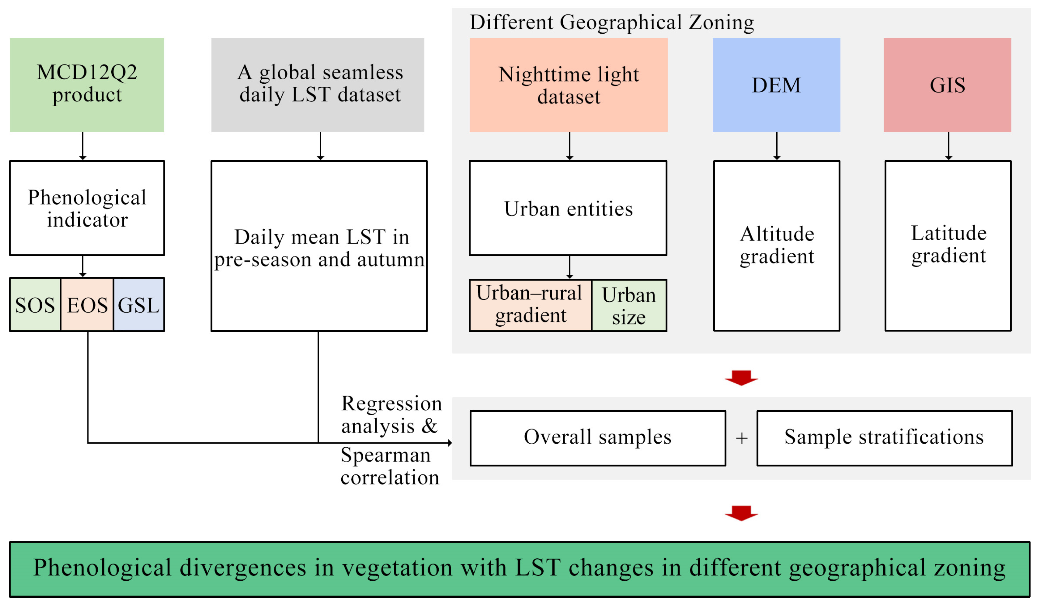
2. Materials and Methods
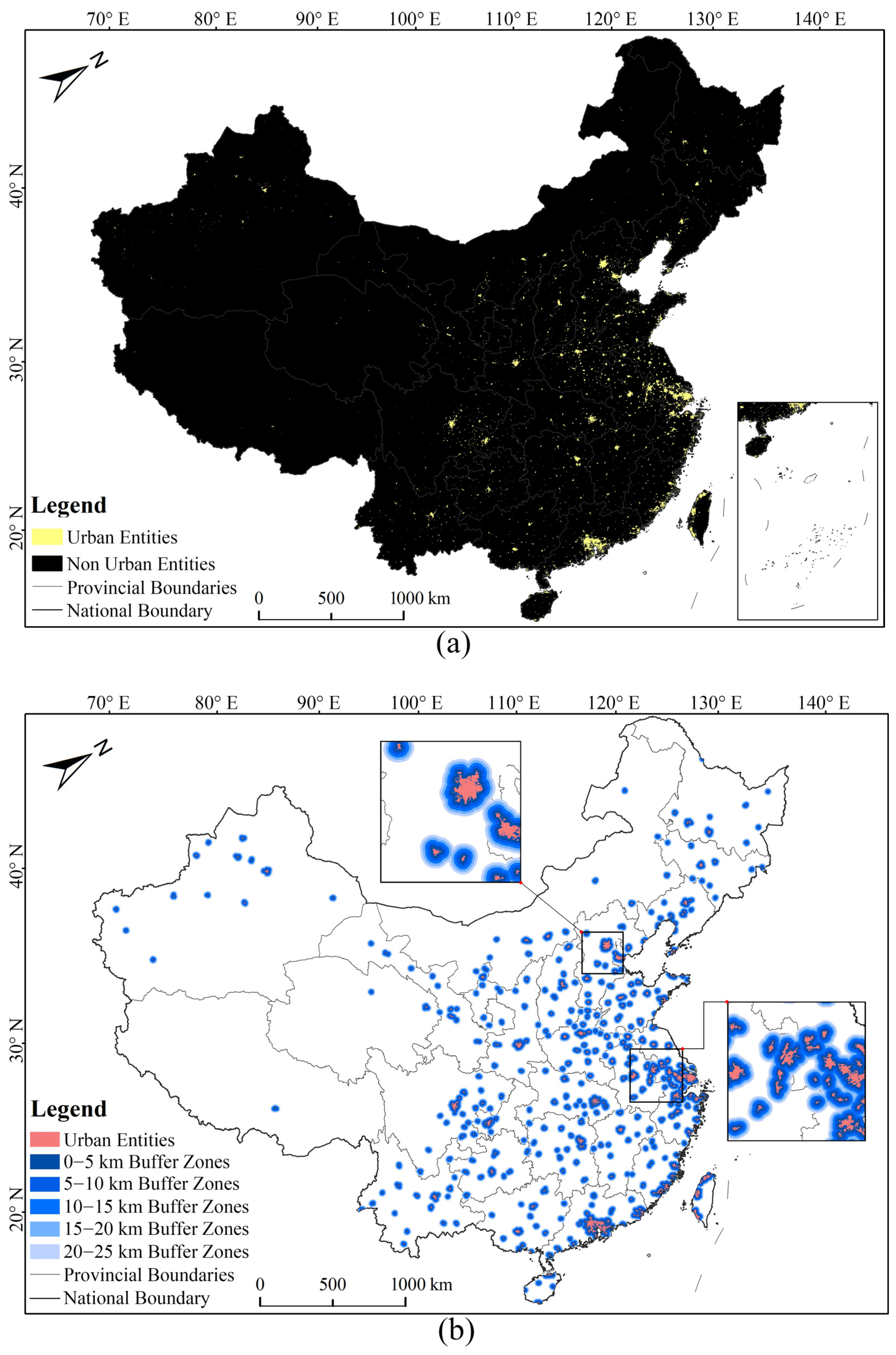
2.1. Study Area

Since 2015, China has surpassed other countries in the world to become the country with the largest urbanization area and diversified urban scale [25,30,52]. China spans a wide range of climate and latitude zones, from tropical, to cold, to temperate; meanwhile, China also has a wide range of altitude spans, with the Qinghai–Tibet Plateau being the highest altitude region in the world [53,54]. Therefore, China is an ideal research area for this study (Figure 1).

2.2. Selected Urban Entities and Urban–Rural Regional Division

The urban entity data were sourced from the Yangtze River Delta Science Data Center, National Earth System Science Data Sharing Infrastructure, and the National Science & Technology Infrastructure of China (http://geodata.nnu.edu.cn (accessed on 5 December 2024)). These data used the difference in light radiation values to determine the background of urban and non-urban entities, with a spatial resolution of 500 m, and the nighttime light dataset involved was sourced from the HAVARD Dataverse (https://dataverse.harvard.edu (accessed on 5 December 2024)) (Figure A1a).
Firstly, since the phenological data in this study was derived from MODIS with a spatial resolution of 500 m, we selected urban entities with an area greater than 10 km2 as study samples, based on the references from previous studies [42,55]. Secondly, we excluded urban entities that lacked phenological observations within their boundaries. Ultimately, 337 urban entities were selected (Figure 1).
In this study, a distance-related urban–rural gradient approach was utilized [34,42,56]. We established a buffer zone of 0–25 km at 5 km intervals on the outskirts of 337 cities to represent the urban–rural gradient related to distance. However, since the boundaries of some cities were less than 25 km apart, the buffer zone of some cities may have overlapped with the boundaries of neighboring cities. As a result, we have merged those closely adjacent cities into urban agglomerations. Finally, we obtained 259 urban agglomerations and their surrounding rural areas (Figure A1b).

2.3. Remote Sensing Observation Data

The remote sensing observation data used in this study mainly included land surface phenology (i.e., SOS, EOS, and GSL), land surface temperature (LST), and digital elevation. In order to match all of the latest available remote sensing datasets, we have focused our study on 2019. The phenological datasets in this study were obtained from the MODIS Land Cover Dynamics (MCD12Q2) products with a spatial resolution of 500 m, which were derived from the time series of the 2-band Enhanced Vegetation Index (EVI2) [57]. In order to reduce the inaccuracy in the subsequent analysis, we removed the extreme values in the phenological datasets based on the threshold method, according to the previous studies [53,55]. Specifically, pixels outside the 30th to the 180th days of the year (DOY) in SOS were removed, and pixels outside the 240th to the 350th DOY in EOS were also removed. The daytime LST data in this study were obtained from a global seamless 1 km resolution daily land surface temperature dataset (2003–2020) (https://doi.org/10.25380/iastate.c.5078492 (accessed on 7 December 2024)). These seamless LST datasets were derived from products of the MOD11A1 and MYD11A1, which were generated by filling in missing pixels through the spatiotemporal information of the original surface temperature data, adopting a spatiotemporal gap-filling framework [58]. In order to fully cover the time series of vegetation phenology as much as possible, we defined 1 December of the previous year to 31 May of the following year as the pre-season, and 1 September to 30 November as the autumn, and then calculated the daily mean LST values for each season [30,59]. The digital elevation model (DEM) used in this study was download from the Institute of Geographic Sciences and Natural Resources Research, CAS, Resource and Environment Science and Data Center (https://www.resdc.cn (accessed on 7 December 2024)) with a spatial resolution of 500 m (Figure 1). Finally, all raster data were resampled to the same spatial resolution of 500 m by a nearest neighbor approach.

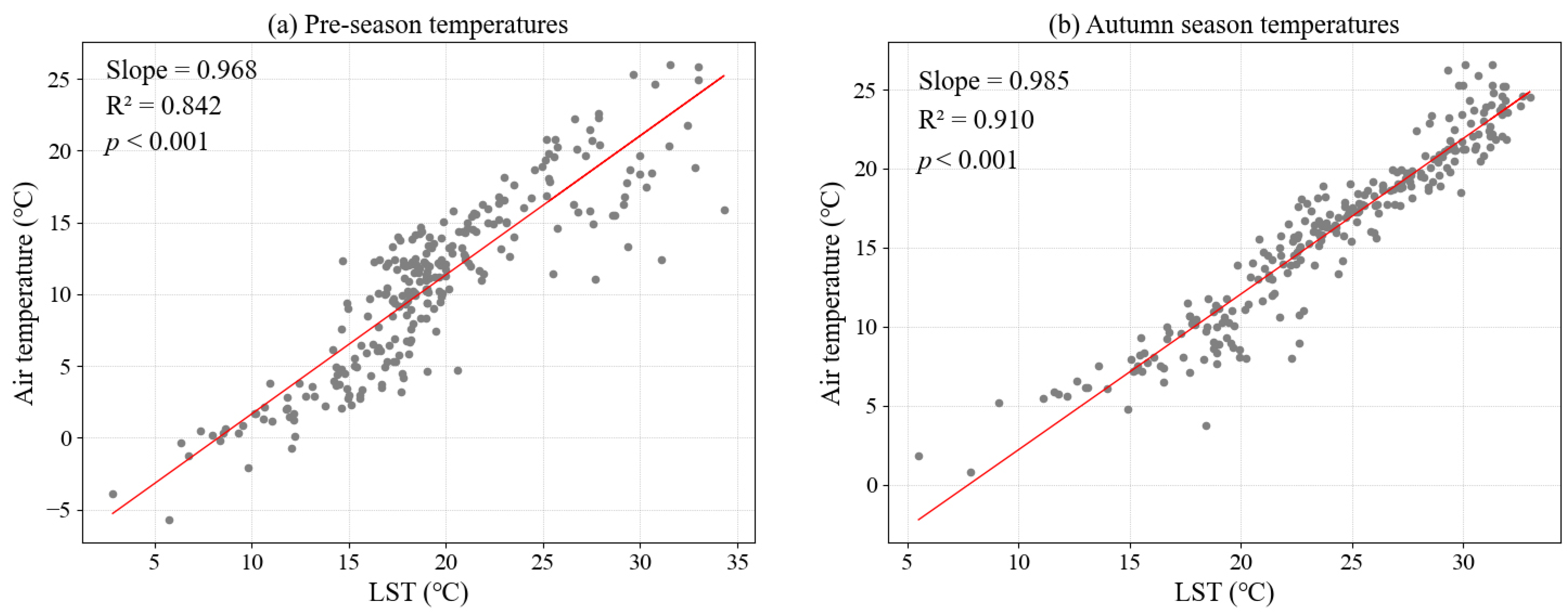
2.4. Quality Control

The MCD12Q2 product was created by assembling the time series of NBAR-EVI2, eliminating outliers and filling dormant period values, fitting a QA/QC-weighted penalized cubic smoothing spline to the time series, identifying valid vegetation cycles within the time series, and then extracting and recording phenometrics for each vegetation cycle. All subsequent functions were applied to a time series of three consecutive years: the product year and the preceding and subsequent years. More detailed information can be found in the user guide to the collection 6.1 MODIS land cover dynamics (MCD12Q2) product (https://lpdaac.usgs.gov/documents/1417/MCD12Q2_User_Guide_V61.pdf (accessed on 21 February 2025)).
The method for the LST dataset in this study included data pre-processing and spatiotemporal fitting. In the data pre-processing, the researchers filtered pixels with a low data quality and filled gaps using the observed LST at another three time points on the same day. In the spatiotemporal fitting, first they fitted the temporal trend (overall mean) of the observations based on the day of the year (independent variable) in each pixel using the smoothing spline function. Then, they spatiotemporally interpolated the residuals between the observations and the overall mean values for each day. Finally, the missing values of LSTs were estimated by adding the overall mean and interpolated residuals. The cross-validation with different missing rates at the global scale indicated that the gap-filled LST data had high accuracy, with an average root mean squared error (RMSE) of 1.88 °C for mid-daytime (13:30) [58].
In addition, previous studies have shown that compared to air temperature, LST may have a more direct effect on vegetation phenology, just as it affects vegetation physiological characteristics [60]. Therefore, we fitted the LSTs and air temperatures of the two seasons within 259 urban agglomerations to supplement the evidence for selecting LSTs as the study data (Figure A2). The air temperature data were obtained from the Institute of Geographic Sciences and Natural Resources Research, CAS, Resource and Environment Science and Data Center (https://www.resdc.cn (accessed on 7 December 2024)). The workflow of our study is shown in Figure 2.

2.5. Statistical Analysis

In this study, the main statistical methods adopted included the quantile method, linear regression analysis, and Spearman’s correlation analysis. The boxplot was adopted to separately calculate SOS, EOS, and LST along the urban–rural gradient. We performed linear regression between LST and SOS and EOS in various urban–rural gradients and altitude zones to quantify the effects of LST on vegetation phenology. Linear regression can also be seen in SOS, EOS, and GSL vs. urban sizes, latitudes, and altitudes. Spearman’s correlation analysis was used to explore the relationships between LST and SOS and EOS in different urban sizes and latitude zones.
In order to conduct a more thorough analysis of the phenological divergences in vegetation with LST changes in different geographical zones, we have stratified samples from 259 urban agglomerations based on urban size, latitude, and altitude (Table 1 and Table 2). It must be mentioned that due to the habitability constraints of high-altitude regions, the number of cities in these areas tends to be relatively lower. Therefore, all urban agglomerations were grouped according to their altitudes and sample quantity, aiming to avoid errors caused by sample quantity and altitude itself. Here, we adopted two grouping rules. One was that the mean altitude distribution of urban agglomerations in each group was relatively equal, but the number of urban agglomerations in each group was uneven. Another was that the number of urban agglomerations in each group was relatively equal, but the mean altitude distribution of urban agglomerations in each group was uneven.

3. Results

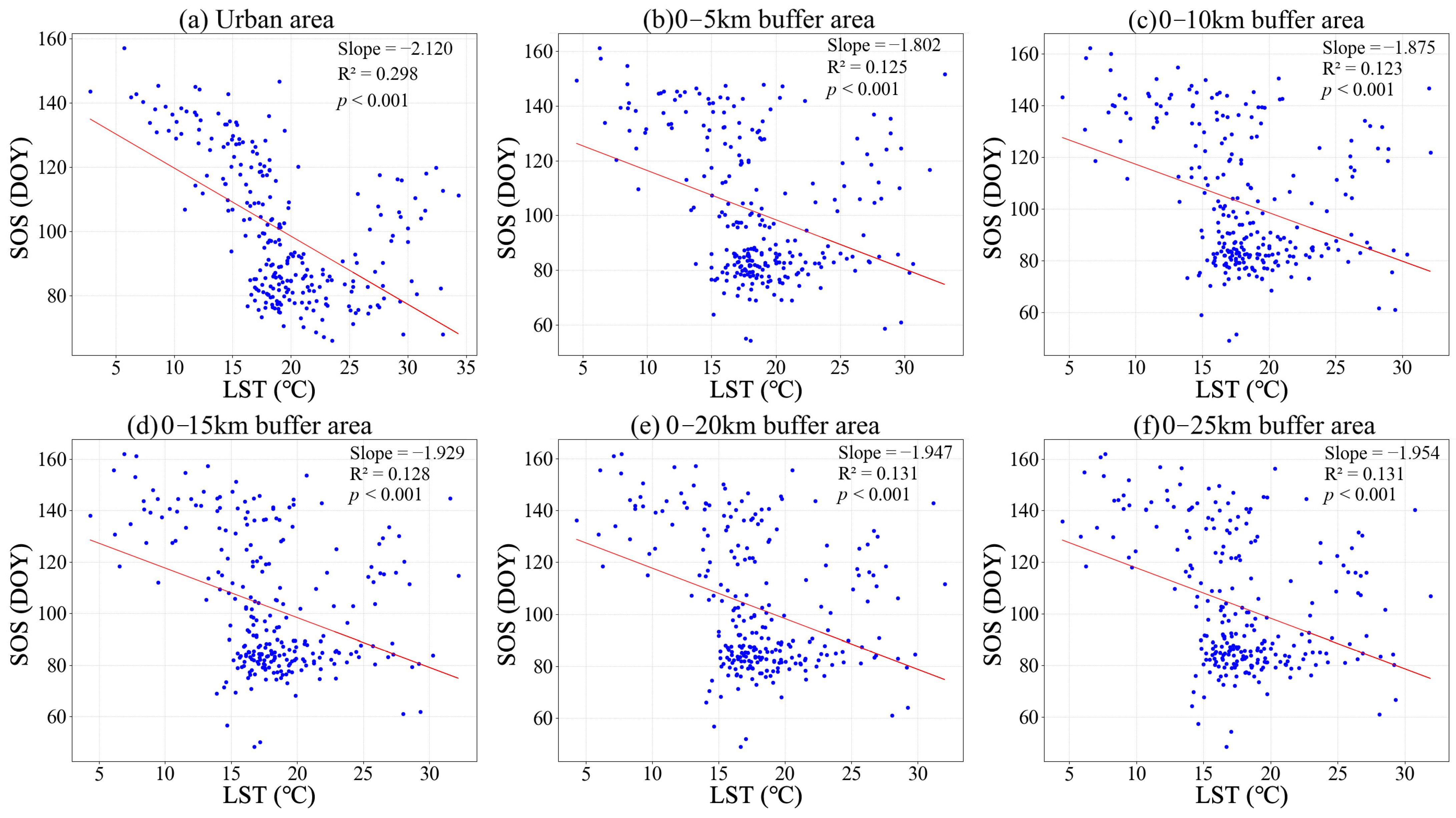
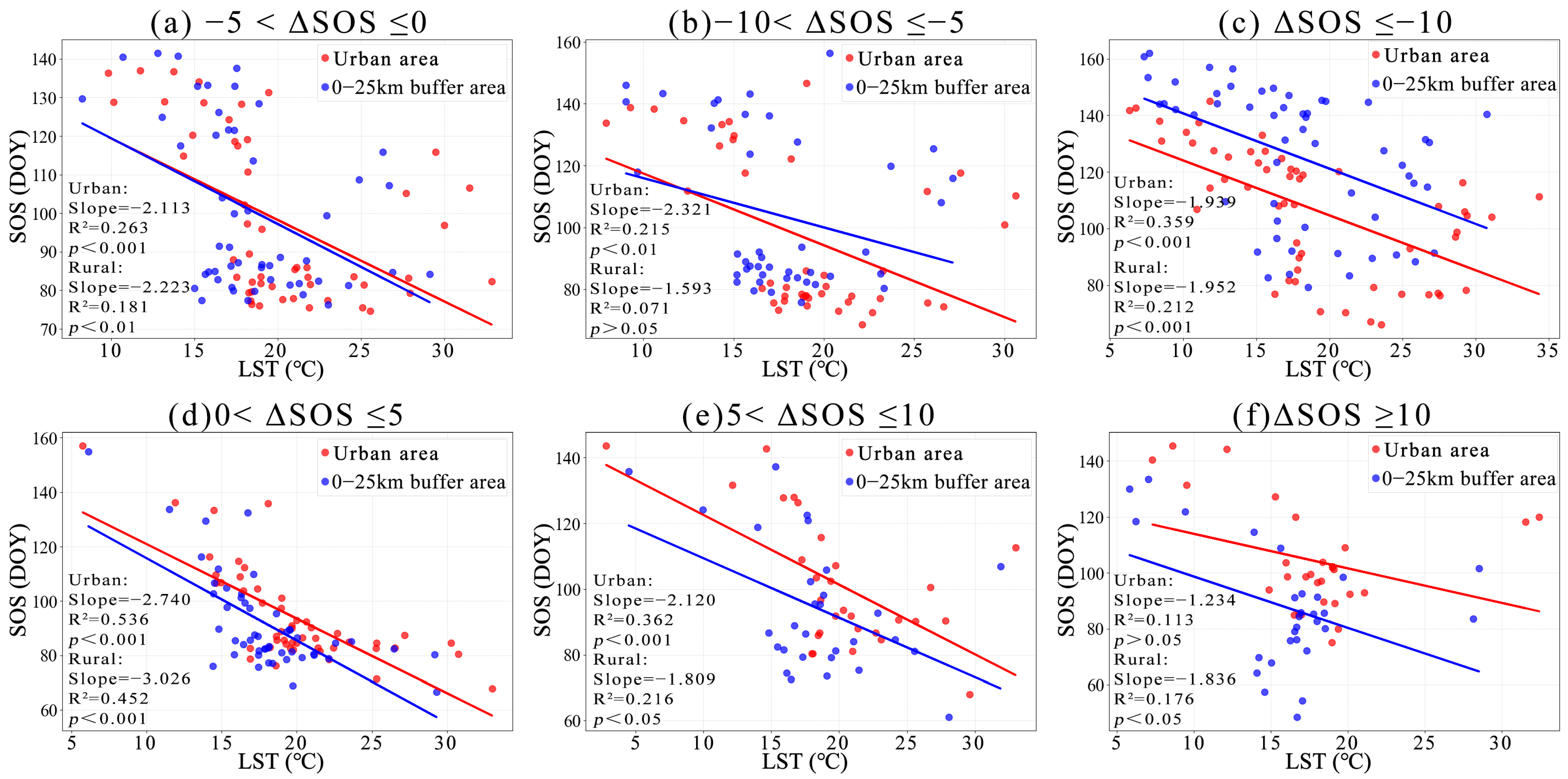
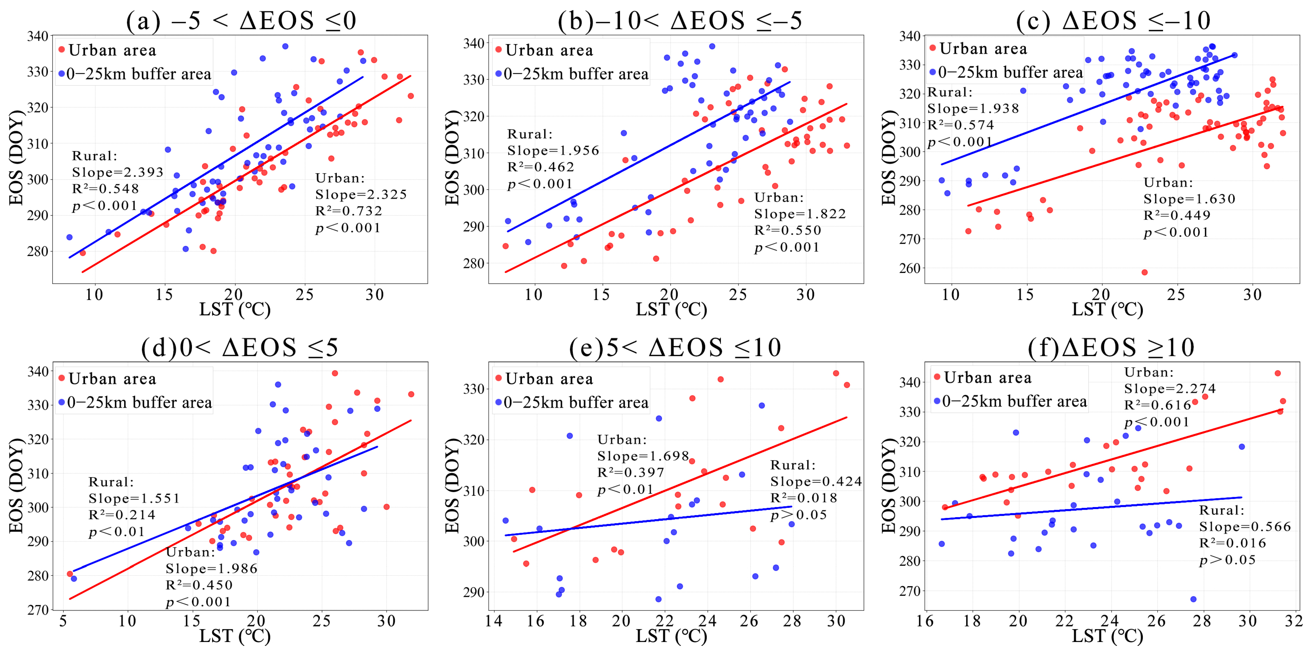
3.1. Phenological Divergences in Vegetation with Temperature Changes Along Urban–Rural Gradient

There were significant differences in vegetation phenological characteristics along the urban–rural gradient (Figure 3). Overall, the mean SOS in urban areas was 1.04 days earlier than that in rural areas, and continued to be delayed along the urban–rural gradient. In contrast, the mean EOS in urban areas was significantly earlier than that in rural areas, and advanced with increasing distance from the urban boundaries. The change trends in the mean GSL along the urban–rural gradient were similar at EOS. Furthermore, it can be observed that the change amplitudes of SOS, EOS, and GSL in the 10–25 km buffer zones were much smaller than those in the urban and 0–10 km buffer zones, and their medians, 25th, and 75th percentiles were quite close (Figure 3a–c), indicating that vegetation phenology was relatively stable in rural areas over 10 km away from urban boundaries. Similarly, the pre-season and autumn LST changes in the 10–25 km buffer zones were also minimal (Figure 3d,e).
Both SOS and EOS in urban and rural areas were significantly correlated with LST (Figure 4 and Figure 5). Specifically, the pre-season LST in both urban and rural areas had negative effects on SOS, especially in urban areas where this effect was the strongest (the slope’s absolute and R2 values were both the highest, at 2.120 and 0.298, respectively) (Figure 4a). It is worth mentioning that as the rural edges expanded, although R2 changed relatively stably, the slope change amplitudes became gradually smaller (Figure 4b–f). This indicated that as the distance from the urban edge increased, the rise in the pre-season LST may have contributed to an earlier SOS, but the effect gradually weakened. Compared to SOS, the effects of autumn LST on EOS were more robust, with R2 even reaching 0.479 in urban areas, but the slope was the lowest at only 1.797 (Figure 5a), indicating that the delayed effect of autumn LST on EOS in rural areas was stronger than that in urban areas. As the distance from the urban edge increased, the delayed effect of autumn LST on EOS gradually weakened (Figure 5b–f).
The relationships between urban–rural vegetation phenology and LST were quantified under different ΔSOS (SOSurban − SOSrural) and ΔEOS (EOSurban − EOSrural). In Figure 6a, according to the slope values, although the advanced effect of the pre-season LST on urban SOS was a little weaker than rural SOS, because of the UHI effect, the urban SOS may have still been earlier than the rural SOS. However, in Figure 6c, the advanced effect of pre-season LST on urban SOS was similar to rural SOS, indicating that the UHI effect may not be the main reason why the urban SOS was much earlier. In Figure 6d, it can be seen that pre-season LST had a stronger advanced effect on the rural SOS. In Figure 7a–c, according to the slope values, the delayed effects of autumn LSTs on the rural EOS became stronger and stronger than their effects on the urban EOS (the difference in slope became larger and larger); at the same time, R2 values were generally high. This result indicated that autumn LST may be the main reason why the urban EOS was earlier than the rural EOS.

3.2. Phenological Divergences in Vegetation with LST Changes in Different Urban Size Zones

As the size of the urban agglomerations changed, the vegetation phenology showed different trends, although these trends were not very obvious or significant. Specifically, SOS decreased with the increase in urban size, while GSL increased and EOS changed insignificantly (Figure A3a–c). In addition, we calculated the mean SOS, EOS, and GSL of all urban agglomerations at every 0.1 (log10 urban size) interval and quantified the linear relationships between urban size and SOS, EOS, and GSL. The result showed that the change in urban size had significant effects on vegetation phenology. With the expansion in urban size, SOS decreased, while EOS and GSL increased (Figure A3d).
Table 3 shows the relationships between SOS and EOS and LST in different urban size zones. Overall, in different urban size zones, the Spearman correlations between EOS and autumn LST were generally higher than those between SOS and pre-season LST. It is worth mentioning that the Spearman correlation coefficients were much higher in urban agglomerations with areas of 0–20 km2 and 200–400 km2 compared to urban agglomerations with other areas. This result indicated that in small and large–medium sized cities, vegetation phenology may be more strongly influenced by LST.

3.3. Phenological Divergences in Vegetation with LST Changes Along Latitude Gradient

As latitude increased, SOS showed a delayed trend, while EOS and GSL showed delayed and prolonged trends, respectively. Overall, at the national level, urban SOS advanced from the north to south in sequence, while EOS and GSL were delayed and extended, respectively (Figure A4). Furthermore, we discovered that nearly 40% of urban agglomerations had a later SOS than rural areas, mostly being concentrated along the southeastern coast and in the 30–40° N region. In the large urban agglomerations such as the Beijing–Tianjin–Hebei urban agglomeration, Yangtze River Delta region, and the Guangdong–Hong Kong–Macao Greater Bay Area, the urban SOS was generally 1–5 days earlier than the rural SOS (Figure A5a). Less than 35% of urban agglomerations had a later EOS than rural areas, and they were mostly distributed in the 30–40° N region. In the 20–30° N region, most of the urban EOS were more than 5 days earlier than the rural EOS (Figure A5b). About 46.3% of urban agglomerations had a longer GSL than rural areas, and the majority of urban agglomerations whose GSL exceeded those in rural areas by 20 days were located in northwest China (such as Xinjiang Uyghur Autonomous Region, Gansu Province, Ningxia Hui Autonomous Region, and western Inner Mongolia Autonomous Region) (Figure A5c). Although the vegetation phenology exhibited regular changes along the latitude gradient, the effects of LST on vegetation phenology seemed to be less similar. In the 18–30° N and 35–50° N regions, the relationships between vegetation phenology and LST were completely opposite (Table 4).

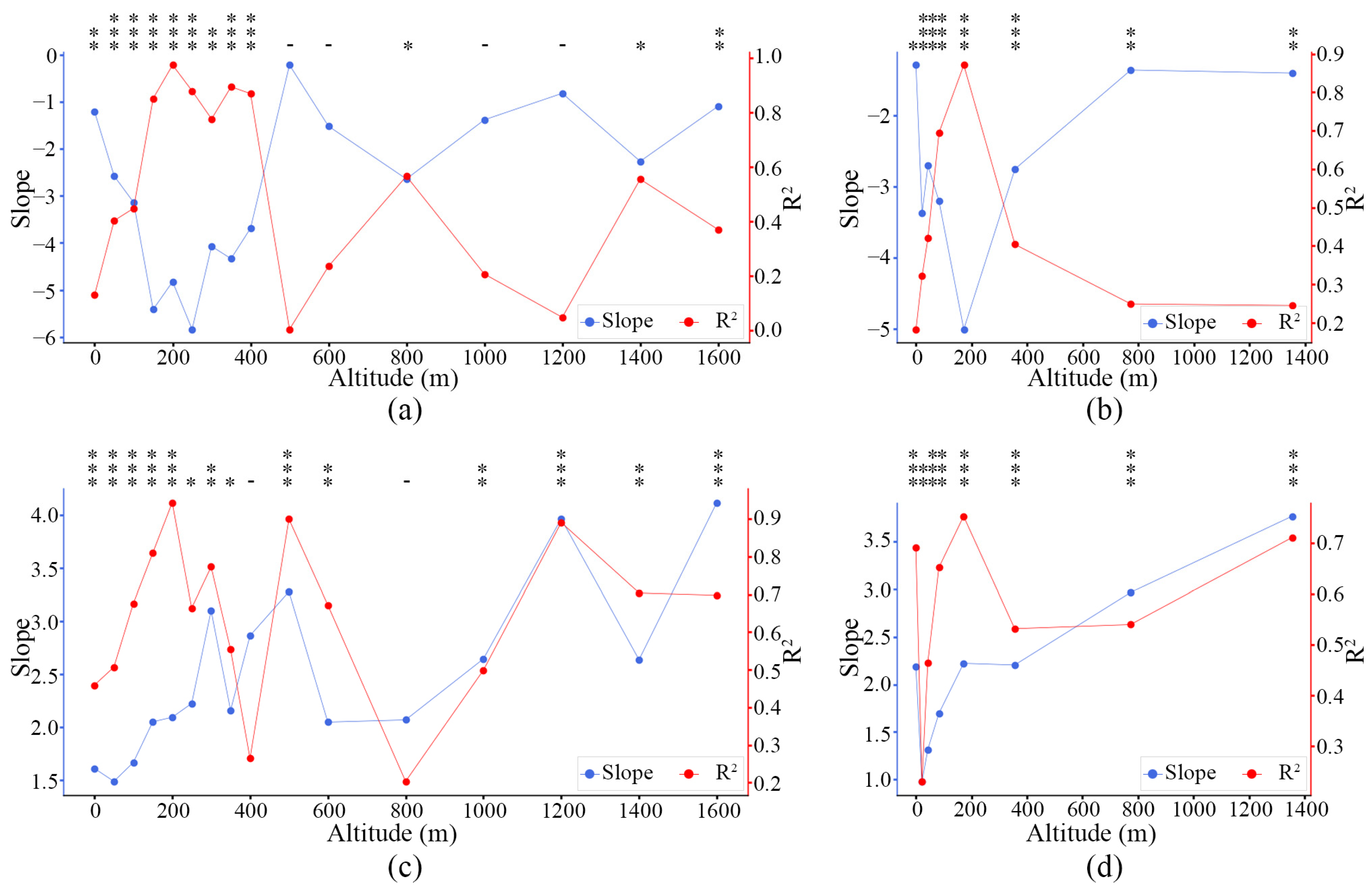
3.4. Phenological Divergences in Vegetation with LST Changes Along Altitude Gradient

In order to verify the relationships between vegetation phenology and altitude, we arranged the mean altitudes of all urban agglomerations from high to low, and then divided them into multiple bins for analysis. We set three bin widths, which were 26 bins (each bin contained ten urban agglomerations), 52 bins (each bin contained five urban agglomerations), and 87 bins (each bin contained three urban agglomerations). The results indicated that as altitude increased, SOS exhibited an upward trend, EOS did not change significantly, and GSL exhibited a downward trend (Figure A6).
On the premise of ensuring significance, in terms of SOS vs. pre-season LST, the larger the R2 values and the smaller the slope values, the stronger the effect of pre-season LST on SOS. It can be seen that the 4th to 9th points (Figure 8a) and the 5th point (Figure 8b) met these conditions, indicating that pre-season LST played a dominant role in advancing SOS at altitudes of 150–500 m and 172–356 m, respectively (Table 2). In terms of EOS vs. autumn LST, the larger the R2 values and slope values, the stronger the effect of autumn LST on EOS. Similarly, it can be seen that the urban agglomerations which met this condition were mainly distributed in areas with altitudes of 170–350 m and above 1200 m (Figure 8c,d).

4. Discussion

UHI refers to the phenomenon where urban temperatures are higher than those in the surrounding rural areas [61]. In our study, we did find that LST gradually decreased along the distance related to the urban–rural gradient (Figure 3d,e). However, the changes in the urban and rural vegetation phenology were not symmetrical with LST changes (Figure 3a–c). Among them, the change trends of EOS and GSL were both consistent and contradictory to many previous studies [26,62,63]. This result further confirmed that temperature was one of the main factors affecting vegetation phenology, but sometimes it was not decisive due to the different geographical zones [17,18,19,27,29].
So far, there have been few studies depicting the response intensity of vegetation phenology to LST along distance-related urban–rural gradients [25]. In this study, we quantified the effects of LST on the phenological divergences in urban and rural vegetation. From the perspective of urban–rural gradients, the advanced effects of pre-season LST on SOS were the strongest in urban areas, and then gradually increased from near to far in rural areas (Figure 4). Studies have indicated that that SOS can be delayed even under suitable temperature conditions when soil moisture content was insufficient [64]. In warm and humid areas, SOS was usually more sensitive to pre-season LST [65]. The interaction between precipitation and other climatic factors contributed significantly to the changes in vegetation phenology [66]. Another study has found that nighttime light intensity can reduce the sensitivity of vegetation phenology to temperature [67,68]. These studies may help to explain why the effects of pre-season LST on SOS gradually increased along the urban–rural gradient, possibly due to the lack of artificial irrigation in rural vegetation, the increased evapotranspiration caused by the UHI effect, and the gradually decreasing nighttime light intensity. The delayed effects of autumn LST on EOS were the weakest in urban areas, and then gradually weakened from near to far in rural areas (Figure 5). The reason for this phenomenon may be that high temperatures in summer and autumn accelerated the rate of evapotranspiration, reduced the soil moisture content, stressed the plant leaf senescence, and caused plants to enter the dormancy period early [69,70,71]. Another possible reason may be that the warming environment promoted higher vegetation productivity, contributing to earlier carbon limitation and EOS [15,51].
In order to further explore the effects of LST on vegetation phenology, we quantified the phenological divergences along different latitude gradients with LST changes. The results indicated that in the high-latitude region of China, pre-season LST had an advanced effect on SOS and a delayed effect on EOS, while in the low-latitude region, these effects seemed to reverse. Specifically, in the 18–30° N region, pre-season LST had a positive effect on SOS (Table 4), and in the southeastern coastal region, urban SOS occurred later than rural SOS (Figure A5a). A previous study also found a similar phenomenon, where SOS changed from an advance to a delay from the middle temperate to southern subtropical zones, while the EOS changed from a delay to an advance [44]. These results all pointed to one problem: continuous high temperatures may lead to delayed SOS. One possible reason is that there was insufficient chilling in the previous summer or winter due to excessively high LSTs, resulting in a reduction in chilling fulfillment, which partly counteracted the forced temperature accumulation in the following year and ultimately caused a delay in SOS [72,73,74,75,76]. In the 18–30° N region, autumn LST had a negative effect on EOS (Table 4). In the 20–35° N region, urban EOS occurred earlier than rural EOS (Figure A5b), and autumn LST had a weaker delayed effect on urban EOS than rural EOS (Figure 7a–c). The other studies have also found that the EOS of most southern cities in the 20–30° N region were earlier than those in rural areas [34,62]. The reason for this phenomenon has been explained in the previous paragraph, which was that the soil water stress caused by high autumn LSTs and the limitation in vegetation productivity may have led to earlier EOS [15,51,69,70,71].
Previous studies have mostly adopted the urbanization intensity or proportion of impervious surfaces to study the UHI effect on vegetation phenology, neglecting the effect of physical distance on the vegetation phenology of urban and surrounding rural areas [25,26]. In this study, we employed a distance-related urban–rural gradient, and found that within the 10–25 km buffer zone, changes in mean SOS, EOS, and GSL slowed down (Figure 3a–c). This result was consistent with previous studies, which suggested that the UHI effect had a significant impact on vegetation phenology within 10 km of the city’s outskirts [53,77,78]. It is also worth noting that the responses of SOS and EOS to LST did not change significantly in rural areas beyond 0–10 km (Figure 4 and Figure 5), which further confirmed this conclusion.
Urban expansion has greatly changed ecosystem structure and is one of the significant factors for the formation of UHI [40,42,79]. Some relevant studies in the United States and China have indicated that the relationship between vegetation phenology and urban size was more significant in large cities [25,26,30]. In our study, we found that vegetation phenology may be more correlated with LST in small cities, but in metropolises, this correlation became weaker or less significant (Table 3). We speculate that smaller cities have lower UHI intensities, and vegetation phenology may be more sensitive to warming, while in metropolitan areas, UHI intensities are higher, and excessively high temperatures may lead to a reversal of vegetation phenology [69,70,75,76].
The effect of altitude on vegetation phenology has been recognized, as it can change the growth environment of vegetation by regulating the climate [20,46]. Our study seemed to supplement this viewpoint to some extent; that is, the effect of pre-season LST on SOS seemed to be less strong in areas with an altitude of 0–150 m, but more strong in areas with an altitude of 150–400 m (Figure 8a,b). This was quite similar to the results of some previous studies. For example, Vitasse et al. [45] proposed that warm winters led to advanced SOS in high-altitude areas, but in low-altitude areas, SOS remained unchanged or even delayed. Li et al. [47] found that SOS was delayed at elevations less than 350 m and increased with rising altitude, and that the primary reason for this may have been that altitude mainly influenced phenological changes by affecting the precipitation and maximum temperature. Adams et al. [80] pointed out that within the altitude range of 204–336 m, the SOS of forests exhibited a nonlinear trend influenced by fluctuations in altitude. Topographic variation was considered to be associated with the corresponding local microclimate [81]. In addition, Xia et al. [20] verified that the delayed speed of EOS caused by the altitude increase reached its maximum value at 1500 m. This further confirmed our study findings that in areas above 1200 m altitude, LST may have a stronger delayed effect on EOS (Figure 8c,d). Previous studies have rarely elucidated how the response intensity of vegetation phenology to LST varies along the altitude gradient, and have not proposed a specific range of altitude. Our study results may largely compensate for the shortcomings of previous studies or confirm certain hypotheses. However, the reasons for the phenological divergences in vegetation with LST changes along the altitude gradient are still unclear, which is an urgent problem requiring research focus in the future.

5. Conclusions

Through zoning based on different urban–rural gradients, urban sizes, latitudes, and altitudes, we explored the phenological divergences in vegetation with LST changes. Our findings can offer the following references for departments involved in land management and landscape planning: (1) It is imperative to pay more attention to the vegetation phenology in urban areas and rural regions beyond 10 km away, as they may be more sensitive to the UHI effect. (2) In urban areas with scant pre-season precipitation and relative aridity, it is crucial to diligently monitor vegetation irrigation to ensure that foliage can unfurl more smoothly under suitable temperatures. Moreover, in urban regions enduring persistent summer heat, it is equally important to provide timely supplemental irrigation to vegetation to avert premature dormancy induced by soil moisture stress. (3) Altitude plays a significant regulatory role in vegetation phenology and its sensitivity to temperature, making it a critical factor to consider in afforestation planning. In addition, our study has revealed that within the context of varying geographical zones, the impact of LST on phenology exhibited significant spatial heterogeneity. This provides strong evidence for the inconsistencies in the trends of phenology observed across previous studies and more relevant constraints for improving vegetation phenology prediction models. In the future, utilizing high-precision observational data and technology to investigate the driving mechanisms behind spatiotemporal divergences in urban phenology is of significant importance.

Author Contributions

Conceptualization, Y.T.; methodology, Y.T. and B.L; software, Y.T.; investigation, Y.T. and B.L.; writing—original draft preparation, Y.T.; writing—review and editing, B.L.; supervision, B.L; project administration, B.L. All authors have read and agreed to the published version of the manuscript.

Funding

This study was supported by the National Natural Science Foundation of China (No. 42171246).

Data Availability Statement

The raw data supporting the conclusions of this article will be made available by the authors on request.

Conflicts of Interest

The authors declare no conflicts of interest.

Appendix A

Figure A1. (a) Map of Chinese urban entities and non-urban entities in 2019 based on nighttime light data, and (b) urban agglomerations and their surrounding 0–25 km rural areas.
Land 14 00562 g0a1
Figure A2. Regression analysis results of LSTs and air temperatures in 259 urban agglomerations in two seasons.
Land 14 00562 g0a2
Figure A3. Scatter plots of relationships between (a) SOS, (b) EOS, (c) GSL, and urban sizes. (d) Scatter plot of the relationship between vegetation phenology and urban size after calculating the mean SOS, EOS, and GSL of all urban agglomerations at every 0.1 (log10 urban size) interval.
Land 14 00562 g0a3
Figure A4. Scatter plot of the relationships between SOS and EOS and latitude.
Land 14 00562 g0a4
Figure A5. Differences in (a) SOS, (b) EOS, and (c) GSL in urban agglomerations and their surrounding 0–25 km rural areas.
Land 14 00562 g0a5aLand 14 00562 g0a5b
Figure A6. Scatter plots of relationships between (a) SOS, (b) EOS, and (c) GSL and altitude under three bin numbers.
Land 14 00562 g0a6

References

  1. IPCC. Summary for Policymakers. 2021. Available online: https://www.ipcc.ch/report/ar6/wg1/downloads/report/IPCC_AR6_WGI_Full_Report_smaller.pdf (accessed on 12 November 2024).
  2. Gill, A.L.; Gallinat, A.S.; Sanders-DeMott, R.; Rigden, A.J.; Gianotti, D.J.S.; Mantooth, J.A.; Templer, P.H. Changes in autumn senescence in northern hemisphere deciduous trees: A meta-analysis of autumn phenology studies. Ann. Bot. 2015, 116, 875–888. [Google Scholar] [CrossRef] [PubMed]
  3. Piao, S.; Liu, Q.; Chen, A.; Janssens, I.A.; Fu, Y.; Dai, J.; Liu, L.; Lian, X.; Shen, M.; Zhu, X. Plant phenology and global climate change: Current progresses and challenges. Glob. Change Biol. 2019, 25, 1922–1940. [Google Scholar] [CrossRef]
  4. Broich, M.; Huete, A.; Tulbure, M.G.; Ma, X.; Xin, Q.; Paget, M.; Restrepo-Coupe, N.; Davies, K.; Devadas, R.; Held, A. Land surface phenological response to decadal climate variability across Australia using satellite remote sensing. Biogeosciences 2014, 11, 5181–5198. [Google Scholar] [CrossRef]
  5. Yang, Y.; Guan, H.; Shen, M.; Liang, W.; Jiang, L. Changes in autumn vegetation dormancy onset date and the climate controls across temperate ecosystems in China from 1982 to 2010. Glob. Change Biol. 2015, 21, 652–665. [Google Scholar] [CrossRef]
  6. Wang, X.; Xiao, J.; Li, X.; Cheng, G.; Ma, M.; Zhu, G.; Arain, M.A.; Black, T.A.; Jassal, R.S. No trends in spring and autumn phenology during the global warming hiatus. Nat. Commun. 2019, 10, 2389. [Google Scholar] [CrossRef] [PubMed]
  7. Li, X.; Du, H.; Zhou, G.; Mao, F.; Zhang, M.; Han, N.; Fan, W.; Liu, H.; Huang, Z.; He, S.; et al. Phenology estimation of subtropical bamboo forests based on assimilated MODIS LAI time series data. ISPRS J. Photogramm. Remote Sens. 2021, 173, 262–277. [Google Scholar] [CrossRef]
  8. Ren, P.; Liu, Z.; Zhou, X.; Peng, C.; Xiao, J.; Wang, S.; Li, X.; Li, P. Strong controls of daily minimum temperature on the autumn photosynthetic phenology of subtropical vegetation in China. For. Ecosyst. 2021, 8, 31. [Google Scholar] [CrossRef] [PubMed]
  9. Piao, S.; Fang, J.; Ciais, P.; Peylin, P.; Huang, Y.; Sitch, S.; Wang, T. The carbon balance of terrestrial ecosystems in China. Nature 2009, 458, 1009–1013. [Google Scholar] [CrossRef]
  10. Tan, J.; Piao, S.; Chen, A.; Zeng, Z.; Ciais, P.; Janssens, I.A.; Mao, J.; Myneni, R.B.; Peng, S.; Penuelas, J.; et al. Seasonally different response of photosynthetic activity to daytime and night-time warming in the Northern Hemisphere. Glob. Change Biol. 2015, 21, 377–387. [Google Scholar] [CrossRef]
  11. Ahlstrom, A.; Xia, J.; Arneth, A.; Luo, Y.; Smith, B. Importance of vegetation dynamics for future terrestrial carbon cycling. Environ. Res. Lett. 2015, 10, 054019. [Google Scholar] [CrossRef]
  12. Li, X.; Du, H.; Zhou, G.; Mao, F.; Zheng, J.; Liu, H.; Huang, Z.; He, S. Spatiotemporal dynamics in assimilated-LAI phenology and its impact on subtropical bamboo forest productivity. Int. J. Appl. Earth Obs. Geoinf. 2021, 96, 102267. [Google Scholar] [CrossRef]
  13. Garonna, I.; de Jong, R.; Stockli, R.; Schmid, B.; Schenkel, D.; Schimel, D.; Schaepman, M.E. Shifting relative importance of climatic constraints on land surface phenology. Environ. Res. Lett. 2018, 13, 024025. [Google Scholar] [CrossRef]
  14. Zohner, C.M. Urbanization phenology and the city. Nat. Ecol. Evol. 2019, 3, 1618–1619. [Google Scholar] [CrossRef] [PubMed]
  15. Zani, D.; Crowther, T.W.; Mo, L.; Renner, S.S.; Zohner, C.M. Increased growing-season productivity drives earlier autumn leaf senescence in temperate trees. Science 2020, 370, 1066–1071. [Google Scholar] [CrossRef]
  16. Guo, M.; Wu, C.; Peng, J.; Lu, L.; Li, S. Identifying contributions of climatic and atmospheric changes to autumn phenology over mid-high latitudes of Northern Hemisphere. Glob. Planet. Change 2021, 197, 103396. [Google Scholar] [CrossRef]
  17. Jeong, S.-J.; Ho, C.-H.; Gim, H.-J.; Brown, M.E. Phenology shifts at start vs. end of growing season in temperate vegetation over the Northern Hemisphere for the period 1982–2008. Glob. Change Biol. 2011, 17, 2385–2399. [Google Scholar] [CrossRef]
  18. Zhao, J.; Zhang, H.; Zhang, Z.; Guo, X.; Li, X.; Chen, C. Spatial and temporal changes in vegetation phenology at middle and high latitudes of the Northern Hemisphere over the past three decades. Remote Sens. 2015, 7, 10973–10995. [Google Scholar] [CrossRef]
  19. Ding, M.; Chen, Q.; Li, L.; Zhang, Y.; Wang, Z.; Liu, L.; Sun, X. Temperature dependence of variations in the end of the growing season from 1982 to 2012 on the Qinghai-Tibetan Plateau. GISci. Remote Sens. 2016, 53, 147–163. [Google Scholar] [CrossRef]
  20. Xia, H.; Qin, Y.; Feng, G.; Meng, Q.; Cui, Y.; Song, H.; Ouyang, Y.; Liu, G. Forest phenology dynamics to climate change and topography in a geographic and climate transition zone: The Qinling Mountains in Central China. Forests 2019, 10, 1007. [Google Scholar] [CrossRef]
  21. Ding, H.; Xu, L.; Elmore, A.J.; Shi, Y. Vegetation phenology influenced by rapid urbanization of the Yangtze Delta region. Remote Sens. 2020, 12, 1783. [Google Scholar] [CrossRef]
  22. Meng, L.; Mao, J.; Zhou, Y.; Richardson, A.D.; Lee, X.; Thornton, P.E.; Ricciuto, D.M.; Li, X.; Dai, Y.; Shi, X.; et al. Urban warming advances spring phenology but reduces the response of phenology to temperature in the conterminous United States. Proc. Natl. Acad. Sci. USA 2020, 117, 4228–4233. [Google Scholar] [CrossRef] [PubMed]
  23. Wang, X.; Du, P.; Chen, D.; Lin, C.; Zheng, H.; Guo, S. Characterizing urbanization-induced land surface phenology change from time-series remotely sensed images at fine spatio-temporal scale: A case study in Nanjing, China (2001–2018). J. Clean. Prod. 2020, 274, 122487. [Google Scholar] [CrossRef]
  24. Li, X.; Zhou, Y.; Asrar, G.R.; Meng, L. Characterizing spatiotemporal dynamics in phenology of urban ecosystems based on Landsat data. Sci. Total Environ. 2017, 605, 721–734. [Google Scholar] [CrossRef]
  25. Jia, W.; Zhao, S.; Zhang, X.; Liu, S.; Henebry, G.M.; Liu, L. Urbanization imprint on land surface phenology: The urban-rural gradient analysis for Chinese cities. Glob. Change Biol. 2021, 27, 2895–2904. [Google Scholar] [CrossRef] [PubMed]
  26. Liu, Z.; Zhou, Y.; Feng, Z. Response of vegetation phenology to urbanization in urban agglomeration areas: A dynamic urban-rural gradient perspective. Sci. Total Environ. 2023, 864, 161109. [Google Scholar] [CrossRef]
  27. Jochner, S.C.; Sparks, T.H.; Estrella, N.; Menzel, A. The influence of altitude and urbanisation on trends and mean dates in phenology (1980–2009). Int. J. Biometeorol. 2012, 56, 387–394. [Google Scholar] [CrossRef]
  28. Lindh, B.C.; McGahan, K.A.; Bluhm, W.L. Changes in urban plant phenology in the Pacific Northwest from 1959 to 2016: Anthropogenic warming and natural oscillation. Int. J. Biometeorol. 2018, 62, 1675–1684. [Google Scholar] [CrossRef]
  29. Donnelly, A.; Yu, R.; Liu, L. Comparing in situ spring phenology and satellite-derived start of season at rural and urban sites in Ireland. Int. J. Remote Sens. 2021, 42, 7821–7841. [Google Scholar] [CrossRef]
  30. Wang, L.; De Boeck, H.J.; Chen, L.; Song, C.; Chen, Z.; McNulty, S.; Zhang, Z. Urban warming increases the temperature sensitivity of spring vegetation phenology at 292 cities across China. Sci. Total Environ. 2022, 834, 155154. [Google Scholar] [CrossRef]
  31. Grimm, N.B.; Faeth, S.H.; Golubiewski, N.E.; Redman, C.L.; Wu, J.; Bai, X.; Briggs, J.M. Global change and the ecology of cities. Science 2008, 319, 756–760. [Google Scholar] [CrossRef]
  32. Youngsteadt, E.; Dale, A.G.; Terando, A.J.; Dunn, R.R.; Frank, S.D. Do cities simulate climate change? A comparison of herbivore response to urban and global warming. Glob. Change Biol. 2015, 21, 97–105. [Google Scholar] [CrossRef]
  33. Zhou, Y. Understanding urban plant phenology for sustainable cities and planet. Nat. Clim. Change 2022, 12, 302–304. [Google Scholar] [CrossRef]
  34. Zhou, D.; Zhang, L.; Hao, L.; Sun, G.; Liu, Y.; Zhu, C. Spatiotemporal trends of urban heat island effect along the urban development intensity gradient in China. Sci. Total Environ. 2016, 544, 617–626. [Google Scholar] [CrossRef] [PubMed]
  35. Qiu, T.; Song, C.; Zhang, Y.; Liu, H.; Vose, J.M. Urbanization and climate change jointly shift land surface phenology in the northern mid-latitude large cities. Remote Sens. Environ. 2020, 236, 111477. [Google Scholar] [CrossRef]
  36. Chapman, S.; Watson, J.E.M.; Salazar, A.; Thatcher, M.; McAlpine, C.A. The impact of urbanization and climate change on urban temperatures: A systematic review. Landsc. Ecol. 2017, 32, 1921–1935. [Google Scholar] [CrossRef]
  37. Krehbiel, C.; Zhang, X.; Henebry, G.M. Impacts of thermal time on land surface phenology in urban areas. Remote Sens. 2017, 9, 499. [Google Scholar] [CrossRef]
  38. Zhang, Y.; Yin, P.; Li, X.; Niu, Q.; Wang, Y.; Cao, W.; Huang, J.; Chen, H.; Yao, X.; Yu, L.; et al. The divergent response of vegetation phenology to urbanization: A case study of Beijing city, China. Sci. Total Environ. 2022, 803, 150079. [Google Scholar] [CrossRef]
  39. Kabano, P.; Lindley, S.; Harris, A. Evidence of urban heat island impacts on the vegetation growing season length in a tropical city. Landsc. Urban Plan. 2021, 206, 103989. [Google Scholar] [CrossRef]
  40. Imhoff, M.L.; Zhang, P.; Wolfe, R.E.; Bounoua, L. Remote sensing of the urban heat island effect across biomes in the continental USA. Remote Sens. Environ. 2010, 114, 504–513. [Google Scholar] [CrossRef]
  41. Giridharan, R.; Emmanuel, R. The impact of urban compactness, comfort strategies and energy consumption on tropical urban heat island intensity: A review. Sustain. Cities Soc. 2018, 40, 677–687. [Google Scholar] [CrossRef]
  42. Li, X.; Zhou, Y.; Asrar, G.R.; Mao, J.; Li, X.; Li, W. Response of vegetation phenology to urbanization in the conterminous United States. Glob. Change Biol. 2017, 23, 2818–2830. [Google Scholar] [CrossRef]
  43. Luo, X.; Zhang, Y.; Sun, D. Response patterns of vegetation phenology along urban-rural gradients in urban areas of different sizes. Complexity 2020, 2020, 7607936. [Google Scholar] [CrossRef]
  44. Ji, Y.; Zhan, W.; Du, H.; Wang, S.; Li, L.; Xiao, J.; Liu, Z.; Huang, F.; Jin, J. Urban-rural gradient in vegetation phenology changes of over 1500 cities across China jointly regulated by urbanization and climate change. ISPRS J. Photogramm. Remote Sens. 2023, 205, 367–384. [Google Scholar] [CrossRef]
  45. Vitasse, Y.; Signarbieux, C.; Fu, Y.H. Global warming leads to more uniform spring phenology across elevations. Proc. Natl. Acad. Sci. USA 2018, 115, 1004–1008. [Google Scholar] [CrossRef]
  46. Yuan, M.; Wang, L.; Lin, A.; Liu, Z.; Li, Q.; Qu, S. Vegetation green up under the influence of daily minimum temperature and urbanization in the Yellow River Basin, China. Ecol. Indic. 2020, 108, 105760. [Google Scholar] [CrossRef]
  47. Li, X.; Du, H.; Zhou, G.; Mao, F.; Zhu, D.; Zhang, M.; Xu, Y.; Zhou, L.; Huang, Z. Spatiotemporal patterns of remotely sensed phenology and their response to climate change and topography in subtropical bamboo forests during 2001–2017: A case study in Zhejiang Province, China. GISci. Remote Sens. 2023, 60, 2163575. [Google Scholar] [CrossRef]
  48. Pepin, N.; Bradley, R.S.; Diaz, H.F.; Baraer, M.; Caceres, E.B.; Forsythe, N.; Fowler, H.; Greenwood, G.; Hashmi, M.Z.; Liu, X.D.; et al. Elevation-dependent warming in mountain regions of the world. Nat. Clim. Change 2015, 5, 424–430. [Google Scholar] [CrossRef]
  49. Liu, W.; Zhang, Q.; Fu, Z.; Chen, X.; Li, H. Analysis and estimation of geographical and topographic influencing factors for precipitation distribution over complex terrains: A case of the Northeast Slope of the Qinghai-Tibet Plateau. Atmosphere 2018, 9, 349. [Google Scholar] [CrossRef]
  50. Xu, M.; Li, X.; Liu, M.; Shi, Y.; Zhou, H.; Zhang, B.; Yan, J. Spatial variation patterns of plant herbaceous community response to warming along latitudinal and altitudinal gradients in mountainous forests of the Loess Plateau, China. Environ. Exp. Bot. 2020, 172, 103983. [Google Scholar] [CrossRef]
  51. Li, D.; Stucky, B.J.; Baiser, B.; Guralnick, R. Urbanization delays plant leaf senescence and extends growing season length in cold but not in warm areas of the Northern Hemisphere. Glob. Ecol. Biogeogr. 2022, 31, 308–320. [Google Scholar] [CrossRef]
  52. Gong, P.; Li, X.; Wang, J.; Bai, Y.; Cheng, B.; Hu, T.; Liu, X.; Xu, B.; Yang, J.; Zhang, W.; et al. Annual maps of global artificial impervious area (GAIA) between 1985 and 2018. Remote Sens. Environ. 2020, 236, 111510. [Google Scholar] [CrossRef]
  53. Zhou, D.; Zhao, S.; Zhang, L.; Liu, S. Remotely sensed assessment of urbanization effects on vegetation phenology in China’s 32 major cities. Remote Sens. Environ. 2016, 176, 272–281. [Google Scholar] [CrossRef]
  54. Liu, J.; Xin, Z.; Huang, Y.; Yu, J. Climate suitability assessment on the Qinghai-Tibet Plateau. Sci. Total Environ. 2022, 816, 151653. [Google Scholar] [CrossRef]
  55. Ren, Q.; He, C.; Huang, Q.; Zhou, Y. Urbanization Impacts on Vegetation Phenology in China. Remote Sens. 2018, 10, 1905. [Google Scholar] [CrossRef]
  56. Yin, P.; Li, X.; Mao, J.; Johnson, B.A.; Wang, B.; Huang, J. A comprehensive analysis of the crop effect on the urban-rural differences in land surface phenology. Sci. Total Environ. 2023, 861, 160604. [Google Scholar] [CrossRef]
  57. Ganguly, S.; Friedl, M.A.; Tan, B.; Zhang, X.; Verma, M. Land surface phenology from MODIS: Characterization of the Collection 5 global land cover dynamics product. Remote Sens. Environ. 2010, 114, 1805–1816. [Google Scholar] [CrossRef]
  58. Zhang, T.; Zhou, Y.; Zhu, Z.; Li, X.; Asrar, G.R. A global seamless 1 km resolution daily land surface temperature dataset (2003–2020). Earth Syst. Sci. Data 2022, 14, 651–664. [Google Scholar] [CrossRef]
  59. Meng, L.; Zhou, Y.; Roman, M.O.; Stokes, E.C.; Wang, Z.; Asrar, G.R.; Mao, J.; Richardson, A.D.; Gu, L.; Wang, Y. Artificial light at night: An underappreciated effect on phenology of deciduous woody plants. PNAS Nexus 2022, 1, pgac046. [Google Scholar] [CrossRef] [PubMed]
  60. De Boeck, H.J.; Van de Velde, H.; De Groote, T.; Nijs, I. Ideas and perspectives: Heat stress: More than hot air. Biogeosciences 2016, 13, 5821–5825. [Google Scholar] [CrossRef]
  61. Voogt, J.A.; Oke, T.R. Thermal remote sensing of urban climates. Remote Sens. Environ. 2003, 86, 370–384. [Google Scholar] [CrossRef]
  62. Qiu, T.; Song, C.; Li, J. Impacts of Urbanization on Vegetation Phenology over the Past Three Decades in Shanghai, China. Remote Sens. 2017, 9, 970. [Google Scholar] [CrossRef]
  63. Zhang, L.; Yang, L.; Zohner, C.M.; Crowther, T.W.; Li, M.; Shen, F.; Guo, M.; Qin, J.; Yao, L.; Zhou, C. Direct and indirect impacts of urbanization on vegetation growth across the world’s cities. Sci. Adv. 2022, 8, eabo0095. [Google Scholar] [CrossRef] [PubMed]
  64. Du, J.; He, Z.; Piatek, K.B.; Chen, L.; Lin, P.; Zhu, X. Interacting effects of temperature and precipitation on climatic sensitivity of spring vegetation green-up in arid mountains of China. Agric. For. Meteorol. 2019, 269, 71–77. [Google Scholar] [CrossRef]
  65. Shen, M.; Piao, S.; Cong, N.; Zhang, G.; Janssens, I.A. Precipitation impacts on vegetation spring phenology on the Tibetan Plateau. Glob. Change Biol. 2015, 21, 3647–3656. [Google Scholar] [CrossRef] [PubMed]
  66. Fu, X.; He, B. Synergistic impacts of built-up characteristics and background climate on urban vegetation phenology: Evidence from Beijing, China. Forests 2024, 15, 728. [Google Scholar] [CrossRef]
  67. Meng, L.; Zhou, Y.; Gu, L.; Richardson, A.D.; Penuelas, J.; Fu, Y.; Wang, Y.; Asrar, G.R.; De Boeck, H.J.; Mao, J.; et al. Photoperiod decelerates the advance of spring phenology of six deciduous tree species under climate warming. Glob. Change Biol. 2021, 27, 2914–2927. [Google Scholar] [CrossRef]
  68. Meng, L.; Zhou, Y.; Li, X.; Asrar, G.R.; Mao, J.; Wanamaker, A.D.; Wang, Y. Divergent responses of spring phenology to daytime and nighttime warming. Agric. For. Meteorol. 2020, 281, 107832. [Google Scholar] [CrossRef]
  69. Estiarte, M.; Penuelas, J. Alteration of the phenology of leaf senescence and fall in winter deciduous species by climate change: Effects on nutrient proficiency. Glob. Change Biol. 2015, 21, 1005–1017. [Google Scholar] [CrossRef]
  70. Vitasse, Y.; Baumgarten, F.; Zohner, C.M.; Kaewthongrach, R.; Fu, Y.H.; Walde, M.G.; Moser, B. Impact of microclimatic conditions and resource availability on spring and autumn phenology of temperate tree seedlings. New Phytol. 2021, 232, 537–550. [Google Scholar] [CrossRef]
  71. Wang, H.; Liu, H.; Cao, G.; Ma, Z.; Li, Y.; Zhang, F.; Zhao, X.; Zhao, X.; Jiang, L.; Sanders, N.J.; et al. Alpine grassland plants grow earlier and faster but biomass remains unchanged over 35 years of climate change. Ecol. Lett. 2020, 23, 701–710. [Google Scholar] [CrossRef]
  72. Chuine, I.; Morin, X.; Bugmann, H. Warming, Photoperiods, and Tree Phenology. Science 2010, 329, 277–278. [Google Scholar] [CrossRef] [PubMed]
  73. Yu, H.; Luedeling, E.; Xu, J. Winter and spring warming result in delayed spring phenology on the Tibetan Plateau. Proc. Natl. Acad. Sci. USA 2010, 107, 22151–22156. [Google Scholar] [CrossRef] [PubMed]
  74. Chen, X.; Wang, L.; Inouye, D. Delayed response of spring phenology to global warming in subtropics and tropics. Agric. For. Meteorol. 2017, 234, 222–235. [Google Scholar] [CrossRef]
  75. Beil, I.; Kreyling, J.; Meyer, C.; Lemcke, N.; Malyshev, A. Late to bed, late to rise-Warmer autumn temperatures delay spring phenology by delaying dormancy. Glob. Change Biol. 2021, 27, 5806–5817. [Google Scholar] [CrossRef]
  76. Yang, L.; Zhao, S.; Liu, S. Urban environments provide new perspectives for forecasting vegetation phenology responses under climate warming. Glob. Change Biol. 2023, 29, 4383–4396. [Google Scholar] [CrossRef]
  77. Zhang, X.Y.; Friedl, M.A.; Schaaf, C.B.; Strahler, A.H.; Schneider, A. The footprint of urban climates on vegetation phenology. Geophys. Res. Lett. 2004, 31, L12209. [Google Scholar] [CrossRef]
  78. Krehbiel, C.P.; Jackson, T.; Henebry, G.M. Web-Enabled Landsat Data Time Series for Monitoring Urban Heat Island Impacts on Land Surface Phenology. IEEE J. Sel. Top. Appl. Earth Observ. Remote Sens. 2016, 9, 2043–2050. [Google Scholar] [CrossRef]
  79. Sun, R.; Lu, Y.; Yang, X.; Chen, L. Understanding the variability of urban heat islands from local background climate and urbanization. J. Clean Prod. 2019, 208, 743–752. [Google Scholar] [CrossRef]
  80. Adams, B.; Matthews, S.; Iverson, L.; Prasad, A.; Peters, M.; Zhao, K. Spring phenological variability promoted by topography and vegetation assembly processes in a temperate forest landscape. Agric. For. Meteorol. 2021, 308, 108578. [Google Scholar] [CrossRef]
  81. Melaas, E.; Friedl, M.A.; Zhu, Z. Detecting interannual variation in deciduous broadleaf forest phenology using Landsat TM/ETM+ data. Remote Sens. Environ. 2013, 132, 176–185. [Google Scholar] [CrossRef]
Figure 1. Spatial distribution of altitude and the selected 337 cities in China.
Land 14 00562 g001
Figure 2. The workflow diagram of this study.
Land 14 00562 g002
Figure 3. Box plots of (a) SOS, (b) EOS, (c) GSL, (d) pre-season LST, and (e) autumn LST along urban–rural gradient. Numbers on each box represent mean values. Top and bottom edges of each box represent 75th and 25th percentiles, respectively.
Land 14 00562 g003
Figure 4. Scatter plots of the relationship between vegetation SOS and pre-season LST along various urban–rural gradients. (a) represents the urban area, and (bf) represent the gradual expansion of the rural edges.
Land 14 00562 g004
Figure 5. Scatter plots of the relationship between EOS and autumn LST along various urban–rural gradients. (a) represents the urban area, and (bf) represent the gradual expansion of the rural edges.
Land 14 00562 g005
Figure 6. Relationships between urban–rural vegetation phenology and LST under different ΔSOS.
Land 14 00562 g006
Figure 7. Relationships between urban–rural vegetation phenology and LST under different ΔEOS.
Land 14 00562 g007
Figure 8. Linear regression parameters (R2 and slope) of SOS and EOS with LST along altitude gradient: (a) SOS vs. pre-season LST according to altitude grouping; (b) SOS vs. pre-season LST according to sample quantity; (c) EOS vs. pre-season LST according to altitude grouping; and (d) EOS vs. pre-season LST according to sample quantity. Notes: “*”, “**”, and “***” denote different significant levels at p < 0.05, p < 0.01, and p < 0.001, respectively; “-” denotes no significance.
Land 14 00562 g008
Table 1. Sample stratification of all urban agglomerations based on urban size and latitude.
Urban Size (km2)Number of Urban AgglomerationsLatitude RangeNumber of Urban Agglomerations
<20 km24518–25° N39
20–50 km26325–30° N70
50–100 km27530–35° N44
100–200 km22635–40° N58
200–400 km22340–50° N48
>400 km227
Table 2. Sample stratification of all urban agglomerations based on altitude and sample quantity.
NO.AltitudeNumber of AgglomerationsAltitude GradientNumber of Agglomerations
The First Grouping RuleThe Second Grouping Rule
10–50 m710–22 m33
250–100 m3522–43 m32
3100–150 m1843–83 m32
4150–200 m1283–172 m32
5200–250 m9172–356 m32
6250–300 m8356–773 m32
7300–350 m7773–1355 m33
8350–400 m9>1355 m33
9400–500 m8
10500–600 m7
11600–800 m11
12800–1000 m10
131000–1200 m15
141200–1400 m12
151400–1600 m9
16>1600 m18
Table 3. Spearman correlation coefficients between SOS, EOS, and LST in different urban sizes.
Urban Size (km2)SOS vs. Pre-Season LSTEOS vs. Autumn LST
<20 km2−0.808 **0.782 **
20–50 km2−0.506 **0.639 **
50–100 km2−0.477 **0.616 **
100–200 km2−0.472 *0.616 *
200–400 km2−0.783 **0.885 **
>400 km2−0.3410.429 *
Note: The “*” and “**” denote different significance levels at p < 0.05 and p < 0.01, respectively.
Table 4. Spearman’s correlation coefficients between SOS and EOS and LST along the latitude gradient.
Latitude RangeSOS vs. Pre-Season LSTEOS vs. Autumn LST
18–25° N0.424 **−0.426 **
25–30° N0.281 *−0.517 **
30–35° N0.203−0.064
35–40° N−0.335 *0.357 **
40–50° N−0.627 **0.588 **
Note: The “*” and “**” denote different significance levels at p < 0.05 and p < 0.01, respectively.
Disclaimer/Publisher’s Note: The statements, opinions and data contained in all publications are solely those of the individual author(s) and contributor(s) and not of MDPI and/or the editor(s). MDPI and/or the editor(s) disclaim responsibility for any injury to people or property resulting from any ideas, methods, instructions or products referred to in the content.

