Article

Study on the Changes of Agritourism Landscape Pattern in Southwest China’s Mountainous Area from a Landscape Function Perspective: A Case Study of Hanyuan County, Sichuan Province

by
Kailu Wang
1,
Yuanzhi Pan
2,*,
Jiao Zhou
1,
Qian Xu
1,3 and
Chenpu Kang
4
1
College of Landscape Architecture, Sichuan Agricultural University, Chengdu 611130, China
2
College of Forestry, Sichuan Agricultural University, Chengdu 611130, China
3
School of Architecture and Planning, Foshan University, Foshan 528225, China
4
Sichuan Forestry and Grassland Survey and Planning Institute, Chengdu 610036, China
*
Author to whom correspondence should be addressed.
Land 2025, 14(12), 2346; https://doi.org/10.3390/land14122346 (registering DOI)
Submission received: 12 November 2025 / Revised: 23 November 2025 / Accepted: 27 November 2025 / Published: 29 November 2025

Abstract

This study investigates the changes and driving mechanisms of agritourism landscapes in mountainous regions of Southwest China, providing a scientific basis for sustainable landscape management. We analyzed Hanyuan County (2013–2023) using remote images, POI data, terrain niche index, distribution index, landscape transition matrix, and logistic regression model from a landscape function perspective. These analyses reveal that the landscape pattern maintains overall stability with local fluctuations, with ecologically oriented landscapes being consistently dominant (>76% coverage). The primary conversion direction of development-potential landscapes shifted from ecological to agricultural dominance after 2018. All landscape types have shown more distinct distribution advantages in the fifth-level terrain gradient, with intensified fluctuations in low-gradient areas after 2018. Location factors were the most common driving force, but their effects differ: production-oriented landscapes shifted from location–climate correlation to location–socioeconomic–terrain correlation; living-oriented landscapes remain influenced by slope and location accessibility; ecological-oriented landscapes shifted from a location–climate correlation to location–tourism correlation; development-potential landscapes were positively influenced by multiple factors. This study suggests implementing zoned management based on functions and terrain gradients through policy guidance and technological intervention. The findings of this study can provide a reference for the comprehensive revitalization of rural areas and the sustainable development of landscapes in similar areas.

1. Introduction

In total, 26% of the global population lives in mountain areas [1], and people in neighboring lowlands also depend on goods and services provided by mountains [2]. Compared to the plains, mountain areas are characterized by slower socioeconomic development and higher out-migration due to accessibility, frequent natural disasters, poorer per capita productive resources, and ecological sensitivity [3,4]. In fact, the significant landscape value of mountains has long coexisted with their inherent developmental fragility, a phenomenon widely recognized in the literature [5,6,7]. In the global mountain development process, the boom in agritourism has provided an important opportunity to address the development dilemmas of mountain areas [8]. European mountain destinations (e.g., the Alps, Apennines, and Carpathians) demonstrate successful models. Comparative studies between Europe and China reveal that, despite differing geographical and cultural contexts, agritourism holds comparable potential to mitigate rural depopulation in Chinese mountains [9]. Under the background of China’s Rural Revitalization Strategy, agritourism fulfills its unique advantage of integrating production, ecology, and livelihood functions. It not only consolidates the results of the battle against poverty with rural revitalization, but also plays a pivotal role in regional ecological protection. Agritourism landscape is a multifunctional system that integrates natural and cultural elements, delivering multiple values including production, ecological, and cultural services [10]. It is widely distributed and highly spatially heterogeneous, consisting of a patchy complex of natural/semi-natural habitat spaces (e.g., farm boundaries, woodlands, ditches, hedgerows, etc.) and human-operated spaces (e.g., farmland, villages, roads, etc.) [11]. However, the complex terrain (e.g., elevation and slope) constraints of mountainous areas profoundly affect the agritourism infrastructure, farming practices, and activity design, which shape the diversity and heterogeneity of the mountain agritourism landscape [12]. These factors constitute fundamental drivers of agritourism landscape pattern changes in mountainous areas.
Currently, relevant studies on landscape pattern changes in mountainous areas are mainly carried out from the perspective of land use, including change characteristics [13,14], driving factors [15], and landscape pattern transition [16]. However, research on mountainous-area agritourism landscapes based on the landscape function perspective has yet to be explored in depth [17]. The landscape function, as an expression of the landscape’s ability to provide goods and services to society [18], arises essentially from the results of interactions between the landscape pattern and ecosystems or elements of the landscape pattern [19]. However, the academic community has not yet formed a unified standard for the classification of landscape functions. Internationally representative classification systems for landscape functions include Costanza [20], Daily [21], de Groot [22], and MA [23]. Building upon these frameworks and adapting to China’s agritourism development context, domestic scholars have generally adopted the functional spatial classification framework of “production-life-ecology” [24,25,26,27]. This framework categorizes the functional core of landscapes into three: production functions that provide agricultural products, living functions that provide aesthetic and cultural services, and ecological functions that provide regulating and supporting services. Even recent studies have begun to explore the agritourism landscape pattern changes and multifunctional value embodiment in mountainous areas, but some limitations remain. On the one hand, the landscape classification mostly follows the land use system and lacks refined approaches based on multiple function orientation. On the other hand, the systematic investigations on the formation mechanism of the functional structure of mountainous areas’ agritourism landscapes under the constraints of terrain are still not in progress. To address these shortcomings, this study, based on the functional framework of “production-life-ecology” and taking into account the characteristics of mountainous areas, classifies mountain agritourism landscapes into four distinct types: production-oriented landscapes (POLs, dominant production function), living-oriented landscapes (LOLs, dominant living function), ecological-oriented landscapes (EOLs, dominant ecological function), and development-potential landscapes (DPLs, dominant multifunctional potential development).
The mountainous areas of Southwest China (including Chongqing, Sichuan, Yunnan, Guizhou, and Tibet) are a representative ecologically and culturally complex and sensitive region, combining typical features of mountain landscapes, rural societies, and minority cultures. As a core component of the region, Sichuan Province is not only one of the most terrain complex areas in China [28], but also an important ecological security barrier in the upper reaches of the Yangtze River [29]. We select Hanyuan County, located in the Hengduan Mountains in western Sichuan Province, which is situated in the transition zone from the Tibetan Plateau to the Sichuan Basin in the east, as a case study. This special geographic environment contributes to the typical development of agritourism in Hanyuan, such as complex human–land relations, and high ecological sensitivity. Therefore, this study takes Hanyuan County as the study area and categorizes the agritourism landscapes in the region from a landscape function perspective and focuses on the following two aspects in combination with the terrain gradient characteristics: (1) the differentiation characteristics of the landscape pattern across terrain gradients; (2) the driving mechanism of the landscape pattern change characteristics. This finding will provide a scientific basis for the landscape optimization and adjustment of agritourism landscape science in the mountainous areas of Southwest China, and moreover, it can provide a reference for the sustainable development of agritourism landscapes in other similar mountainous areas worldwide.

2. Materials and Methodology

2.1. Study Area

Hanyuan is a mountainous county in Southwest China’s Sichuan Province, located between 102°16′ and 103°27′ E and 29°05′ and 29°43 N (Figure 1). The terrain is diverse, dominated by mountainous terrain (elevations between 672 m and 3936 m and slopes between 0° and 79.96°), surrounded by mountains forming a high northwestern and low southeastern area, with a low valley in the center. It has a subtropical monsoon humid climate, with an average annual temperature of approximately 17.9 °C, low and uneven rainfall, and significant vertical changes in climate. But the sunshine is sufficient; the annual sunshine time is 1475.8 h. After the 4.20 Lushan earthquake in 2013, Hanyuan focused on fostering special programs of agritourism in its post-disaster reconstruction efforts [30]. In 2018, as one of the pilot regions for China’s Rural Revitalization Strategy, Hanyuan accelerated the integration and development of agritourism with culture and ecotourism [31]. By 2023, Hanyuan County had emerged as a model region in Sichuan Province with remarkable results in the implementation of the Rural Revitalization Strategy [32], with 528.67 km2 of distinctive agritourism bases and 2709 family farms cultivated.

2.2. Data Source and Preprocessing

2.2.1. Landscape Classification of Agritourism Based on Landscape Function Perspective

The Landsat satellite images used in this study were obtained from two primary sources: the Geospatial Data Cloud platform of the Chinese Academy of Sciences (https://www.gscloud.cn/, accessed on 10 August 2020) and the USGS Earth Explorer (https://earthexplorer.usgs.gov, accessed on 28 November 2023). We acquired the less cloudy image data (resolution of 30 m) of Hanyuan County in the years 2013 (Landsat 7 ETM), 2018 (Landsat 8 OLI), and 2023 (Landsat 8-9 OLI). All images used the WGS _1984_UTM_Zone_48N projected coordinate system. And all remote sensing images were preprocessed using ENVI 5.3 software, including radiometric calibration, atmospheric correction, geometric correction, image cropping, and mosaicking. Then, according to the Chinese Land Use Classification Standard (GB/T 21010-2017) [33], with respect to the landscape functional classification system (described in Section 1) and the field research, we categorized the processed imagery into distinct landscape categories (Table 1). When applying the “production-life-ecology” framework, we were guided by its core land cover foundation: the production and ecological function primarily rely on “natural or semi-natural habitats” (such as cropland, forest land, grassland, and water bodies), differing mainly in their dominant service orientation (product supply or ecological regulation), while the living function is primarily manifested on “artificial construction surfaces” (such as residential, commercial, and infrastructure land). The DPL category specifically comprises land use types with multifunctional potential for future transformation, including sand, bare ground, and other land. “Other land” refers to land types excluding those explicitly assigned to POL, LOL, and EOL, representing areas with undetermined or transitional functions under the national standard. Finally, the Kappa coefficient accuracy validation of the classification results showed that the four-phase decoding accuracy was above 90%, indicating that the classification was reliable. In summary, the four landscape types were defined according to their dominant functions and corresponding land cover foundations: (1) POL mainly provided the production functions, corresponding to natural/semi-natural habitats for agricultural production; (2) LOL emphasized on human living environments with cultural services, primarily corresponding to artificial construction surfaces; (3) EOL focused on natural or semi-natural area for ecosystem maintenance, corresponding to natural/semi-natural habitats with minimal human intervention; and (4) DPL were undeveloped lands with multifunctional potential, whose land cover is also in a natural or semi-natural state.

2.2.2. POI Data Acquisition and Processing

POI (point of interest) data contain spatial location and attribute information of geographic entities, and play an important role in a variety of location-based studies such as social media, navigation, geographic information retrieval tools, and tourism services [34,35]. Furthermore, POI data has demonstrated its value in deep spatial analysis within studies such as high-precision land use classification [36] and urban functional zone identification [37]. In this study, POI data are systematically processed to provide data support for the analysis related to the driving factors of agritourism landscape pattern changes (e.g., distance to dining/lodging, distance to scenic spots, as detailed in Section 2.3.2).
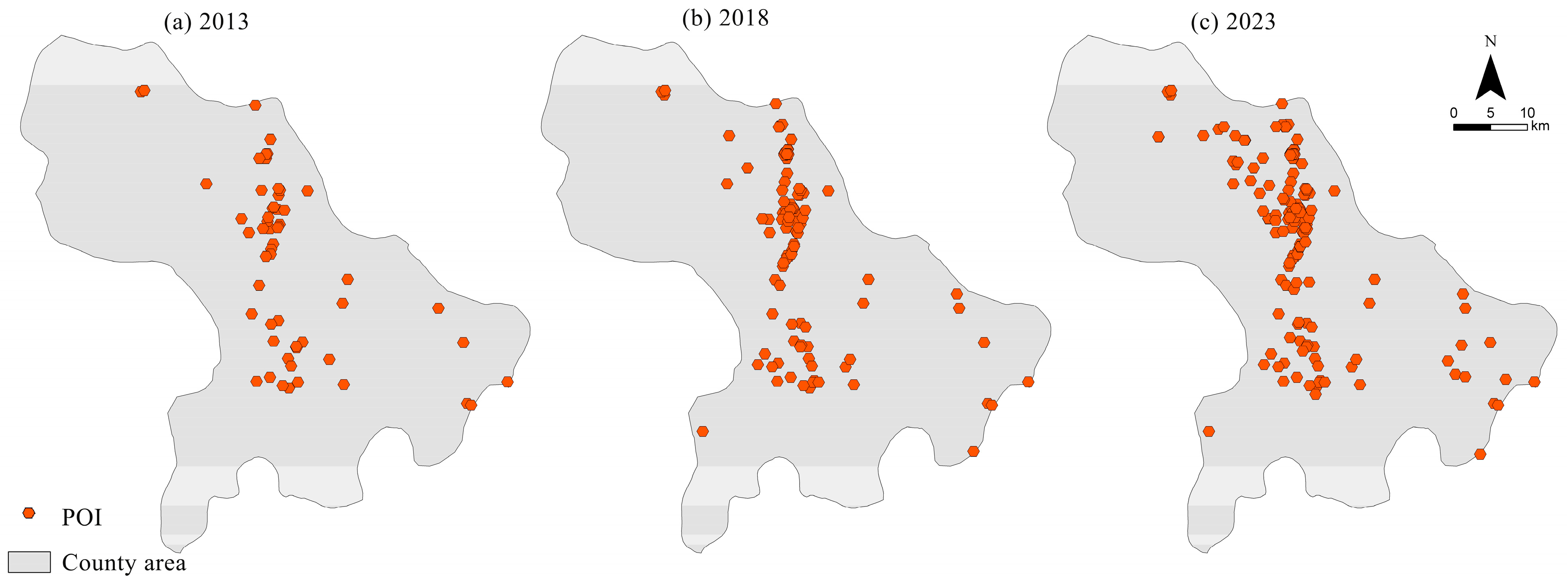
The data processing process includes five key steps. First, initial POI data were obtained on Baidu Map (https://map.baidu.com/, accessed on 29 November 2023) for the periods of 2013, 2018, and 2023. Second, we selected keywords related to agritourism landscape, such as dining/lodging (“farm stays”, “resorts”, and “agriculture-themed homestays”) and scenic spots (“cultural attractions”, “farms”, “agricultural garden”, “pick-your-own orchards”, and “family farm”), for the initial screening of the data. Third, the above keyword search results were verified and supplemented based on the field research information and the business registration information to ensure the completeness of the data. Additionally, we also collected POI data for the administrative centers of the townships. Fourth, the screened and supplemented POI data were corrected for geographic coordinates offset using QGIS 3.22.4 software. Finally, within ArcGIS 10.8, the POI data were converted into point-feature spatial data and unified to the WGS_1984_UTM_Zone_48N projected coordinate system. The final valid POI samples obtained were 57 in 2013, 102 in 2018, and 321 in 2023, as well as 21 POI data for township administrative centers (Figure 2).

2.2.3. Multisource Supporting Data

To comprehensively analyze landscape changes, several complementary datasets were incorporated in addition to the landscape classification system and POI data (Table 2). The Digital Elevation Model (DEM) was processed using ArcGIS 10.8 software to obtain terrain indices such as elevation, slope, etc., to provide a database for terrain gradient zoning (Section 2.3.1). Road network and meteorological data (2013–2023) were similarly utilized for study area extent cropping and calculation using ArcGIS 10.8 software to be used for driving factor analysis (Section 2.3.2). All the above spatial datasets were uniformly sampled at a resolution of 30 m, and the projected coordinate system was converted to WGS_1984_UTM_Zone_48N. In addition, specific indicators of each township, such as population, food production, industry proportion, etc., were extracted and calculated from the socioeconomic data of 2013–2023, to provide multidimensional data support for the driving mechanism of landscape pattern changes.

2.3. Methodology

2.3.1. Landscape Pattern Differentiation Characteristics Across Terrain Gradients

(1) Terrain Niche Index (TNI)
DEM is a reliable method to represent continuously changing terrain features in a study area [38]. Elevation and slope were calculated to form TNI using ArcGIS 10.8 software. The relationship between TNI, elevation and slope are as follows: (1) the higher the elevation is, the greater the slope is, and the greater the TNI will be, and vice versa; (2) in other conditions, for example, high elevation but small slope, low elevation but large slope, or elevation and slope in the middle value, the TNI approaches the middle value. The TNI can be expressed as follows:
T = log [ ( E / E ¯ + 1 ) × ( S / S ¯ + 1 ) ]
where T represents the TNI; E and S represent the elevation value and slope value of a location, respectively; and E ¯ and S ¯ represent the average elevation value and average slope value in the study area, respectively.
(2) Terrain Zoning
Based on the topographic and geomorphic features of Hanyuan, the TNI was classified into five terrain gradients according to the Jenks optimization (Table 3). Then the graded TNI layers were overlaid with the layers of landscape types to calculate the area of each landscape type on different terrain gradients. The above zoning and calculations were performed in ArcGIS 10.8 software.
(3) Distribution Index (DI)
To eliminate the dimensional differences caused by the different areal proportions of each landscape type, the DI indicates the distribution frequency of different landscape types at different TNI gradients [14]. The DI can be expressed as follows:
P = ( S i e / S i ) / ( S e / S )
where P represents the DI; S i e is the area of landscape type i at terrain gradient e ; S i is the area of landscape type i ; S e is the area of terrain gradient e ; and S is the study area. If the P value is greater than 1, then landscape type i is the dominant landscape type at terrain gradient e . The greater P is, the more obvious the distributional advantage of landscape type i at terrain gradient e .
(4) Single Landscape Dynamic Degree
The single landscape dynamic degree quantifies the change rate of a single landscape type’s area in a certain time range [39]. The data source is the area of each landscape type obtained by calculation using ArcGIS 10.8 software. The calculation formula is as follows:
K s = U b U a U a × 1 T × 100 %
where K s indicates the dynamic attitude of a landscape type in the study period; U a and U b indicate the initial and final areas of the landscape type, and T is the study period duration (in years).
(5) Analysis of Landscape Changes and Transitions
To visualize spatiotemporal landscape changes and quantify their transformation pathways, we performed spatial overlay analysis in landscape type maps from 2013, 2018, and 2023 in ArcGIS 10.8. This process generated maps of dynamic landscape changes, delineating areas where transitions occurred between the two study periods. Subsequently, we extracted landscape transition matrices from the overlay results. To clearly present the dominant pathways and the stability of each landscape type, these matrices reported the transition probability (in percentage), which represented the proportion of each initial landscape type’s total area that was converted to every other type.

2.3.2. Driving Mechanism Analysis

(1) Driver factors selection and preprocessing
Landscape pattern change is notably influenced by both natural factors and human activities [40]. Earlier studies have made significant advances in exploring the relationship between landscape patterns and driving factors [41,42,43,44]. However, it is worth noting that there is often a high correlation between many driving factors, and too many factors are prone to cause the problem of multicollinearity, leading to variable redundancy [45]. This study systematically selects driving factors based on three criteria: (1) reliable and easily accessible data sources; (2) quantifiable and independent of each other; (3) multidimensional coverage (ten dimensions such as population, living standards, food security, agricultural technology, etc.). Based on the regional characteristics of the study area and related literature [39,46,47], we finally selected a total of 12 driving factors (Table 4). Non-spatial data, including socioeconomic factors (X1–X3), were calculated based on acquired socioeconomic data. Spatial data, including location (X4-X5), tourism (X6–X8), climate (X9–X10), and terrain (X11–X12), were calculated using ArcGIS 10.8 based on spatial data such as road networks, POI, landscape classifications, DEM, and meteorological data.
(2) Logistic regression model
Traditional linear regression exhibits inherent limitations in analyzing discrete dependent variables. On the contrary, logistic regression effectively solves the problem of driver modeling for categorical variables through the probability transformation mechanism, and is widely used in landscape driver studies [39,48]. In this study, we designated landscape change values (changed labeled as 1 and unchanged labeled as 0) for the periods 2013–2018 and 2018–2023 as the dependent variable. In addition, we conducted stratified random sampling using ArcGIS 10.8 to obtain 560 valid sample points from the landscape change raster maps to ensure sufficient sample size and reduce the effect of spatial autocorrelation, with the continuous values of each driver factor as independent variables. In addition, we conducted stratified random sampling using ArcGIS 10.8 to obtain 560 valid sample points from the landscape change raster maps to ensure sufficient sample size and reduce the effect of spatial autocorrelation. All driving factor values were extracted and standardized uniformly before analysis. Also, to avoid multicollinearity among driving factors that could compromise model stability and reliability, we conducted Variance Inflation Factor (VIF) tests. With the criterion of VIF < 5, we performed iterative variable selection on all independent variables separately for the two periods using SPSS 27 until the VIF values of all remaining variables were below 5 (Table S1).
The analysis was conducted in SPSS 27 to identify dominant driving factors for four landscape types in two periods. We used the Wald statistic to test the regression coefficients of the model. Regression coefficients were evaluated using Wald statistics. If the probability (p) value is less than the given significance level α (α = 0.05), then the null hypothesis should be rejected and the linear relationship between the independent variables and the probability should be considered significant. As well, a larger Wald statistic indicated that the driving factor exerted a more significant influence on landscape type changes. Moreover, the positive or negative sign of the regression coefficient (β) indicated the direction of change in landscape types driven by each factor. Model fit was assessed using the Hosmer–Lemeshow (HL) and area under the ROC curve (AUC) tests, where p > 0.05 and AUC > 0.7 indicated a satisfactory model fit.

3. Results

3.1. Spatiotemporal Dynamics of Agritourism Landscape Types

3.1.1. Temporal Changes in Landscape Types

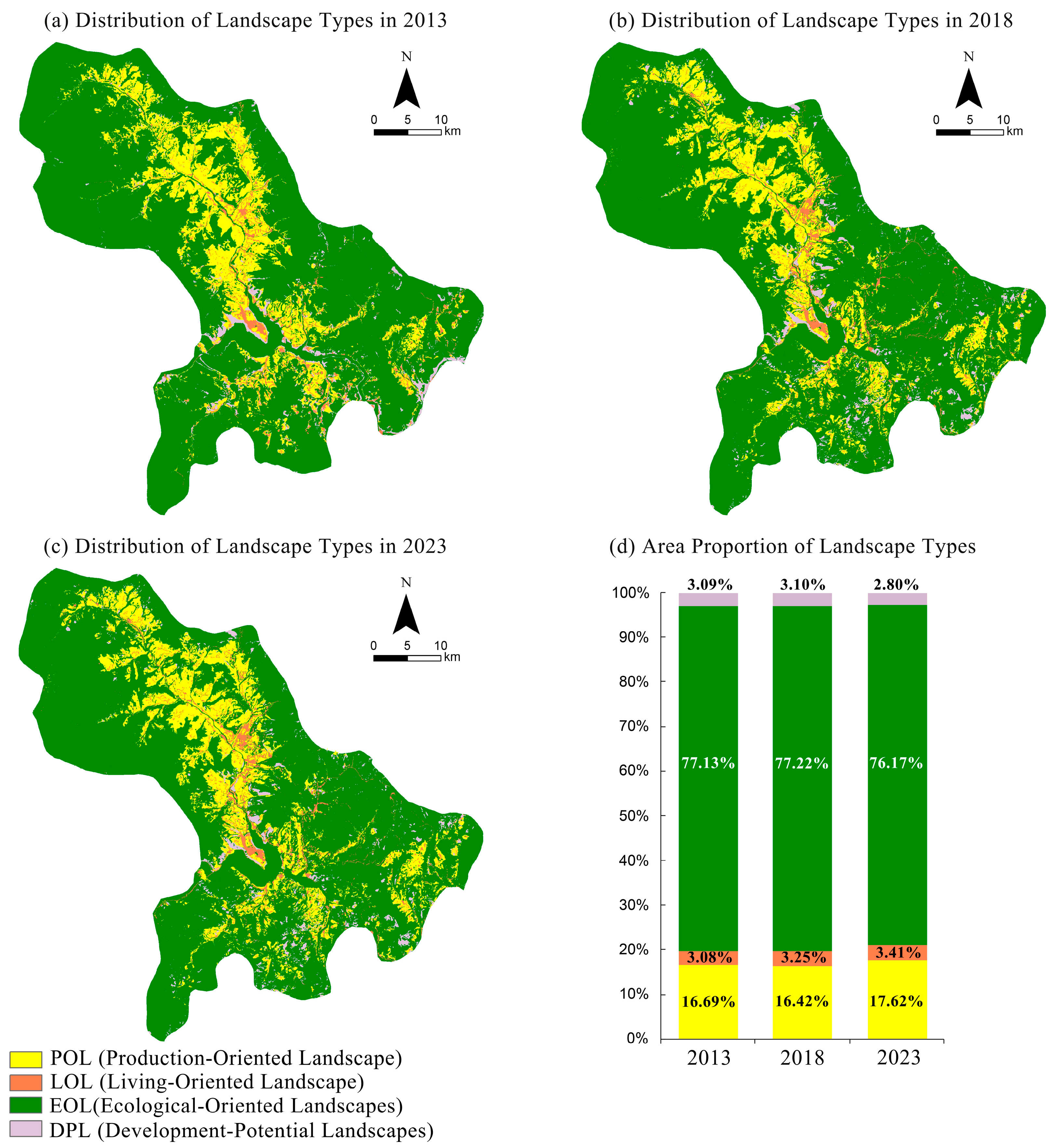
As shown in Figure 3, the study area agritourism landscapes in all three periods (2013, 2018, and 2023) showed obvious stratified distribution characteristics. EOL persistently dominant (>76% coverage) followed by POL (16–18%). Spatially, POL and LOL clustered in the central core area, while EOL formed concentric buffers surrounding them, and DPL was scattered in the form of patches. Chronologically, the proportion of each landscape type fluctuated around 1%, indicating that the stratification structure has a strong stability.
The analysis of the landscape dynamic attitude presented obvious stage characteristics (Table 5). During 2013–2018, EOL remained relatively stable (the attitude of 0.0002%), reflecting its stability as a landscape matrix, while POL showed negative growth (the attitude of −0.3240). In contrast, LOL and DPL exhibited positive expansion (the attitude of 1.1031% and 0.0770%, respectively). During 2018–2023, POL reversed the trend with a rapid increase in area (attitude of 3.6637%), while LOL continued to increase (attitude of 2.3467%). Both EOL and DPL experienced area reduction, particularly DPL, which showed a significant decline (attitude of −4.9627%).
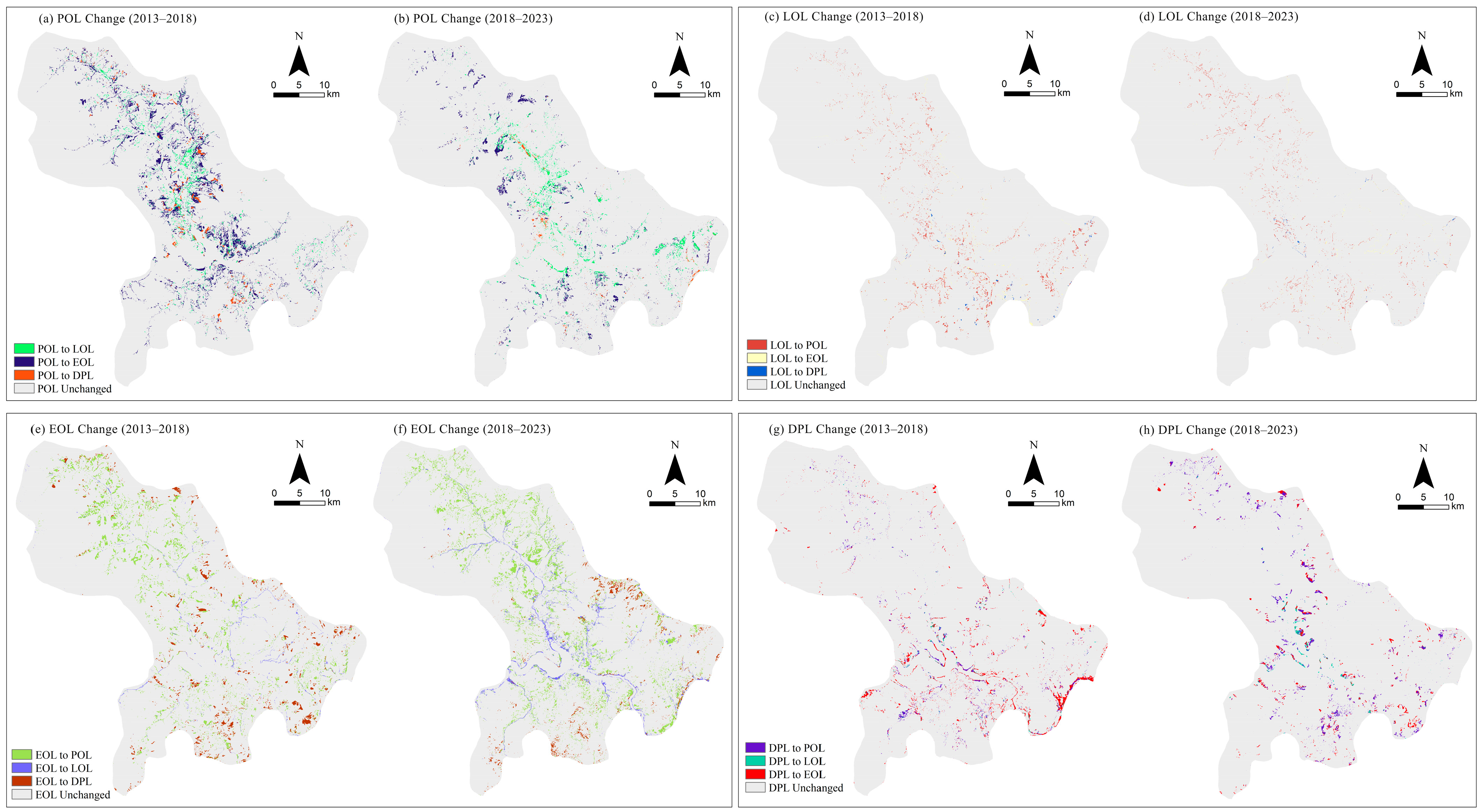
By spatially overlaying the landscape types from the two periods, we identified their spatial transition characteristics (Figure 4). The percentage transition ratio matrix from 2013 to 2018 (Table 6) and from 2018 to 2023 (Table 7) reveal mutual transformations between all landscape types.
POL transitions were mainly distributed in the central and northern parts of the study area (Figure 4a,b). Its stability increased, with the proportion of unchanged areas rising from 65.09% (2013–2018) to 80.28% (2018–2023). Its main conversion in the first period was to EOL (24.72%), shifting to conversions to LOL (8.05%) and EOL (9.89%) in the second period. LOL transitions expanded from the north (2013–2018) to the north–central (2018–2023) (Figure 4c,d). Its stability significantly increased, with the proportion of unchanged rising from 48.23% to 70.89%. Across both periods, the primary transfer destination remained POL (32.84% and 18.74%, respectively). EOL, as the dominant type, exhibited high stability, with its unchanged proportion consistently higher than 90% (Figure 4e,f). Its transitions were widely distributed, with the primary direction of transfer being POL (4.94% in the previous period and 6.78% in the latter period). DPL was the most dynamically changing type, with unchanged proportions below 30% (Figure 4g,h). Its transition areas shifted from the north (2013–2018) to the southeast, northeast, and central regions (2018–2023). In the previous period, it primarily shifted to EOL (47.30%), while in the latter period, it mainly shifted to POL (37.65%).

3.1.2. Spatial Distribution Along Terrain Gradients

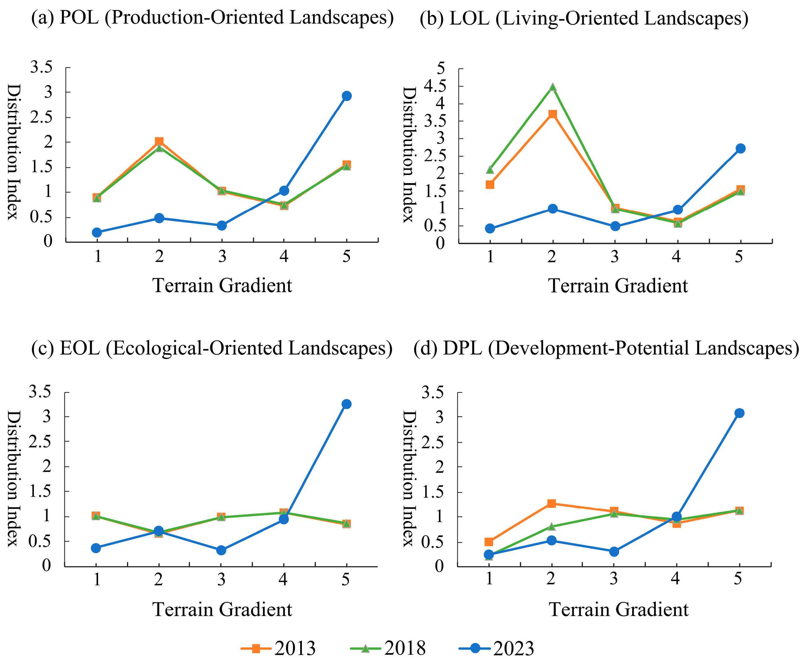
The vector terrain gradient map was overlaid with landscape type distribution maps of three periods (Figure 3) in ArcGIS 10.8 to calculate distribution indices for each landscape type across terrain gradients (Figure 5). Results revealed distinct distribution patterns in 2023 compared to the two earlier periods. During 2013 to 2018, POL and EOL exhibited largely consistent trends in distribution index changes, while LOL and DPL showed minor fluctuations within terrain gradient levels 1 to 2. LOL increased within these two gradient levels, whereas DPL displayed the opposite trend. By 2023, all landscape types demonstrated significantly stronger distribution advantages in terrain level 5 compared to 2013 and 2018. Across other terrain gradients, distribution index trends varied by landscape type: POL and LOL decreased markedly in levels 1–3 but began to rise in level 4; EOL declined noticeably in levels 1 and 3; and DPL decreased in levels 2 and 3. Overall, terrain gradient levels 1, 2, 3, and 5 exhibited more frequent fluctuations in landscape type changes.

3.2. Key Factors Associated with Landscape Types

To ensure model stability, we conducted multicollinearity tests (VIF < 5) for the driving factors in each study period (see Table S1 for iterative screening results). The logistic regression models run on this basis demonstrated varying performance.
For the period 2013–2018, all drivers were retained. During this period, all models were tested for the HL and area under the ROC curve tests, reaching acceptable standards (p > 0.05 and AUC > 0.7), indicating reliable model results.
For the period 2018–2023, logistic regression models were constructed after excluding the two factors with high VIF values: “annual mean temperature (X9)” and “elevation (X11)”. The HL test for all models in this period met the standard (p > 0.05), but the AUC values for all models ranged between 0.6 and 0.7. This indicates that the filtered set of drivers for this period provides some indicative value for explaining the spatial patterns of landscape change, but the overall predictive capacity of the models remains moderate.

3.2.1. Factors Associated with Production-Oriented Landscapes (POLs)

After excluding independent variables with p-values above 0.05, the regression results for each driver are presented in Table 8.
During 2013 to 2018, the key factors associated with POLs were primarily associated with location and climate, in the order of: distance to dining/lodging (X6) > annual mean temperature (X9) > annual mean precipitation (X10) > distance to township center (X5). Specifically, POLs showed a negative correlation with distance to dining/lodging (X6), distance to township center (X5), and annual mean precipitation (X10), and a positive correlation with annual mean temperature (X9).
From 2018 to 2023, the key driving factors identified by our model were primarily associated with socioeconomic, location, climate, and terrain, in the following order: distance to township center (X5) > distance to nearest road (X4) > year-end cultivated land area (X3) > annual mean precipitation (X10) > slope (X12). In this period, POLs correlated negatively with distance to township center (X5) and slope (X12), and positively with year-end cultivated land area (X3), distance to nearest road (X4), and annual mean precipitation (X10).

3.2.2. Factors Associated with Living-Oriented Landscapes (LOLs)

As shown in Table 9, During 2013 to 2018, the key factors of LOL changes were associated with socioeconomic, locational, tourism, climate, and terrain factors, in the following order: slope (X12) > year-end cultivated land area (X3) > distance to scenic spots (X7) > distance to township center (X5) > annual mean temperature (X9) > distance to nearest road (X4). Specifically, LOLs showed negative correlations with year-end cultivated land area (X3), distance to nearest road (X4), distance to township center (X5), and slope (X12), but positive correlations with distance to scenic spots (X7) and annual mean temperature (X9).
From 2018 to 2023, the key driving factors identified by our model of LOL were mainly linked to socioeconomic, locational, climate, and terrain factors, ranked as follows: slope (X12) > annual mean precipitation (X10) > population density (X1) > distance to nearest township center (X5). In this period, LOL exhibited negative correlations with all three drivers.

3.2.3. Factors Associated with Ecological-Oriented Landscapes (EOLs)

As shown in Table 10, during 2013 to 2018, the key factors associated with EOL changes were mainly associated with location and climate factors, ranked as follows: annual mean precipitation (X10) > distance to nearest road (X4). Specifically, EOLs exhibited a negative correlation with annual mean precipitation (X10) but a positive correlation with distance to nearest road (X4).
From 2018 to 2023, the identified potential drivers of EOL shifted to location and tourism factors, in the following order: distance to township center (X5) > distance to scenic spots (X7). In this period, EOL showed a negative correlation with distance to scenic spots (X7) and a positive correlation with distance to the township center (X5).

3.2.4. Factors Associated with Development-Potential Landscapes (DPLs)

As shown in Table 11, during 2013 to 2018, the key factors associated with DPL changes were associated with location, tourism, climate, and terrain factors, ranked as follows: annual mean precipitation (X10) > annual mean temperature (X9) > distance to dining/lodging (X6) > distance to township center (X5) > slope (X12). Specifically, DPLs exhibited a negative correlation with annual mean temperature (X9), but positive correlations with distance to township center (X5), distance to dining/lodging (X6), annual mean precipitation (X10), and slope (X12).
From 2018 to 2023, the identified potential primary drivers of DPL involved tourism and terrain factors, in the following order: slope (X12) > distance to water bodies (X8). In this period, DPL showed positive correlations with both driving factors.

4. Discussion

4.1. Spatiotemporal Changes in Agritourism Landscape Pattern

The spatiotemporal changes in the agritourism landscape in Hanyuan County exhibit characteristics of “overall structural stability and localized periodic fluctuations.” As the dominant landscape type in the study area, EOLs consistently account for over 76% of the total area. It effectively maintains the fundamental framework of regional ecological security. EOLs exhibited exceptional stability (over 90% of their area remains unchanged). Notably, the DPL, as the most dynamic type, underwent a significant shift in its primary conversion direction between the two periods: it primarily transitioned to EOL (47.30%) from 2013 to 2018, but shifted to primarily converting to POL (37.65%) from 2018 to 2023. This shift indicates that the earlier phase, dominated by ecological restoration processes, increasingly gave way to agricultural expansion in the later period. Analysis of the terrain gradient in landscape patterns further indicates that the distribution advantage of EOL in terrain gradient level 5 continues to increase. In contrast, POL and LOL are primarily distributed in levels 1 to 3. Studies in the Hantai District of Shanxi [49] and the Taihang Mountain [50] similarly indicate that due to the dual constraints of terrain conditions and ecological protection policies, EOL is more concentrated in areas with complex terrain. Furthermore, the fluctuation range of the overall landscape pattern in mountainous areas is significantly smaller than that in areas with gentle terrain. This collectively indicates that complex terrains may impose physical constraints on the spatial division of different landscape functions.
In addition, the POL and LOL are concentrated in the central low-terrain gradient areas. And the EOL is distributed around the peripheral high terrain gradient areas. This “core-periphery” landscape space pattern remained stable from 2013 to 2023. This spatial pattern is also similar to the distribution patterns of human settlements and ecological landscape observed in the Hani terraced fields area of Yunnan [13] and the karst mountainous area of Guizhou [51]. It indicates that in the mountainous area of Southwest China with complex terrain, human activities are often spatially restricted by the natural environment. However, different from the above two study areas, the EOL forms a more complete “surround” boundary for POL and LOL in Hanyuan County. The formation of this unique spatial form may be closely related to the systematic ecological fragility of the local dry–hot valley, as well as the conscious strengthening of ecological conservation functions during the development of its agritourism and the implementation of the Rural Revitalization Strategy. From a landscape function perspective, the essence of this landscape pattern is the physical manifestation of the competition and balance among the four major functions of production, living, ecology, and expansion in space. By 2023, the distribution advantages of each landscape type in terrain gradient level 5 had significantly strengthened, while they fluctuated frequently in terrain gradient levels 1 to 3. It indicates that the intensity of human activities increased in the low terrain gradients. This phenomenon contrasts with the general trend of continuous increase in the intensity of human activities in most plain areas [52,53,54]. However, it echoes the “contraction and concentration” pattern of human activities in mountainous areas discovered in Fengjie County, which is also located in the southwestern mountainous region [55]. Both findings reveal that some mountainous areas are undergoing a two-level differentiation of “modern mountainous landscapes”: the high terrain gradient areas are dominated by natural landscapes, while the low terrain gradient areas are dominated by modern agricultural landscapes, thus forming an ecological and economic landscape pattern in the vertical space [56].

4.2. Driving Mechanisms Underlying Landscape Changes

The landscape pattern changes in mountainous areas are jointly influenced by the natural environment, socioeconomic development, and human factors [56]. The logistic regression results reveal the type heterogeneity and temporal difference in the driving mechanism of landscape pattern changes in Hanyuan County agritourism from 2013 to 2023. The most notable feature is the high and widespread correlation of the location factor.
Firstly, location factors are the primary correlation-driven categories for the dynamic changes in the four landscape types, but their modes of action show a distinct functional orientation. Except for the DPL during 2018 to 2023, all other landscape types were influenced by at least one location factor in both periods. Specifically, POL’s drivers shifted from “location-climate correlation” to “location-socioeconomic-terrain correlation”. During 2013–2018, POL spatial distribution tended to tourism service nodes and areas with good hydrothermal conditions. It reflects the reliance of smallholder specialty agricultural models within the local Rural Revitalization Strategy on the tourism market and favorable natural conditions during implementation. From 2018 to 2023, the spatial distribution of POL tended to be near the township center areas with abundant arable land resources, and the gentle slope areas with suitable precipitation conditions, while far from the main road. This transformation is consistent with the conclusion observed in some areas of agricultural transformation in the mountainous regions of Southwest China that “agricultural landscapes are transforming from self-sufficient and extensive to market-oriented and intensive” [16,57]. The driver factors of LOL are the most complex, involving multiple types of driver factors. It was affected by location (distance to nearest road (X4) and distance to township center (X5)), climate (annual mean temperature (X9) and annual mean precipitation (X10)), and terrain (slope (X12)) in both periods. Against the background of poor local location endowment, LOL showed a high correlation with location accessibility, exhibiting significant neighborhood effects with roads and township centers in its distribution. More importantly, slope (X12) as the primary factor consistently negatively correlated with changes in LOL highlighted that gentle terrain was a prerequisite for realizing its tourism service functions. The highly consistent spatial preferences of both LOL and POL for these superior locations (gentle terrain, proximity to roads, and centrality) create direct competition between them. This powerfully explains why frequent mutual transformations between POL and LOL occur within the landscape transition matrix. The driving factors associated with EOL were from climate (annual mean precipitation (X10)) to location (distance to township center (X5) and distance to scenic spots (X7)), with its spatial distribution tended to move away from the township center and nearby scenic spots. It may be highly related to the conditions of local tourism resources: POI screening of scenic spots in this study area reveals that the core scenic spots (such as Yunding Mountain Scenic Area, Dadu River Canyon National Geopark, agricultural park, picking garden, family farms, etc.) are themselves large natural or semi-natural ecological patches. This phenomenon may be explained by the mechanism of integrating agriculture and tourism promoted by the Rural Revitalization Strategy [31,32,58]: as the ecological background of agritourism, EOL may be influenced by market demand and consequently affects nearby scenic spots, while needing to avoid regions with high human activity intensity (such as township centers) to maintain its fundamental development—high-quality resource endowment. DPL shows a positive correlation with multiple driving factors, indicating that its distribution is correlated with various driving factors and lacks a clear functional orientation. This may lead to its disorder in spatial distribution. This disordered distribution, on the one hand, endows DPL landscape units with the potential to rapidly transform into other landscape types, and on the other hand, poses a potential risk to the ecological continuity and pattern stability of the local landscape.
Secondly, the driving mechanisms of the four landscape types in the study area present critical timing differences. After 2018, with the in-depth implementation of the Rural Revitalization Strategy in Hanyuan County, the integration process of agriculture and tourism accelerated, and the primary drivers linking POL and EOL also underwent a fundamental transformation. It precisely corresponds to the policy positioning of the research area—“compound upgrading of mountainous characteristic agriculture” and “reconstruction of the entire ecosystem”. Meanwhile, terrain factor (such as slope (X12)) was identified as one of the primary factors associated with the spatial patterns of POL, LOL, and DPL. This signifies the fundamental role of terrain conditions in shaping mountainous landscape patterns [59]. From another perspective, this spatial constraint association can also be transformed into an opportunity to shape samples of mountainous characteristic agritourism landscapes under the guidance of policy and the intervention of technology.

4.3. Implications for Sustainable Agritourism Landscape Management

4.3.1. Zoned Optimization Based on Landscape Functions and Terrain Gradients

For production-living areas with high human activity intensity within the terrain gradient 1 to 3, the focus should be on improving land utilization (such as high-standard farmland) and controlling development intensity. Meanwhile, the inheritance, protection, and innovation of local farming folk culture are mainly considered to optimize the living space of people in the areas near township centers. The government should vigorously promote the integrated development model of agriculture and tourism to enhance the cultural connotation and tourism value of agritourism landscapes. For ecological-production areas (dominated by EOL) with low human activity intensity in terrain gradient levels 4 to 5, special attention should be paid to the protection of the ecosystem, preventing the disorderly encroachment of PDL on EOL. At the same time, low-disturbance eco-tourism models and forest economies should be moderately developed.

4.3.2. Policy Guidance and Technological Intervention

Given the high dependence of POL and LOL on location conditions, policies should focus on improving infrastructure services, especially enhancing the connectivity of local transportation networks, in order to reduce production costs to a certain extent. In addition, based on the integration of local agritourism resources, the tourism routes should be planned and improved to achieve the transition and interaction of the “core-periphery” area, so as to enhance the overall tourism appeal [59]. The policy should also focus its optimization efforts on the development and improvement of multifunctional landscape integration areas to achieve a virtuous cycle of rural industrial revitalization. In terms of technological intervention, the resilience of landscape systems can be enhanced by promoting agricultural technological innovation, such as building high-standard farmland in low terrain gradients and implementing three-dimensional agricultural planting models in high terrain gradients. Furthermore, in promoting the specialized smallholder farming model, it is also necessary to emphasize ecological conservation awareness campaigns, technical training, and economic support for farmers. This approach not only encourages farmer participation but also enhances their ecological well-being.

4.4. Limitations and Prospects

This study has several limitations, which also provide directions for future research. A primary focus is that compared to the acceptable predictive accuracy of the 2013–2018 model (AUC > 0.7), the predictive accuracy of the logistic regression model for the 2018–2023 period was generally moderate (0.6 < AUC < 0.7). This phenomenon of models exhibiting varying explanatory power across different periods has been reported in studies of land use change drivers, suggesting it is not an isolated case. For example, Imbrechts et al. [60] similarly described their AUC values ranging from “poor (<0.6) to good (>0.7)” when investigating drivers of landscape transformation in Portugal, indicating that critical explanatory variables might be missing from the driver analysis framework.
For this study, the decline in model performance in later periods likely stems from the selected spatial variables failing to fully capture intensifying socioeconomic dynamics. These may include direct policy interventions, market shifts, and complex human decision-making processes that became more dominant drivers in 2018. Therefore, the factors identified for the 2018–2023 period are interpreted here as primary associated drivers rather than decisive contributing factors.
As a result, future research should privilege the combination of new data sources to capture these complex factors. This may involve employing questionnaire surveys to clarify human decision-making mechanisms, utilizing additional spatial data (such as open social media platforms with geolocation information) to measure economic activity, and applying machine learning techniques to better handle nonlinear relationships and identify key driver interactions.

5. Conclusions

This study takes the agritourism landscape of Hanyuan County as the research object. From a landscape functionality perspective, we analyzed the spatiotemporal characteristics and driving mechanisms of four landscape types across different terrain gradients by combining images and POI data from 2013, 2018, and 2023. The main conclusions are as follows.
Firstly, the spatiotemporal changes in the agritourism landscape in Hanyuan County present the characteristics of “overall stable stability and localized periodic fluctuations “. EOL consistently dominates the primary landscape type within the study area. Its exceptional stability, with over 90% of the area remaining unchanged, forms the regional ecological framework. POL and LOL are mainly concentrated within the central region’s low terrain gradient levels 1 to 3. The three together form a stable “core—periphery” landscape structure. Notably, the change trajectory of the DPL shifted from a primary conversion to EOL (2013–2018) to a dominant conversion to POL (2018–2023), indicating a transition in regional changes from ecological restoration to agricultural expansion. In 2023, the distribution advantages of each landscape type in terrain gradient level 5 were significantly enhanced, while they fluctuated frequently in terrain gradient levels 1 to 3, indicating that the agritourism landscape is undergoing a reconstruction of vertical spatial polarization.
Secondly, the driving mechanism of the changes in the landscape pattern of agritourism in the study area shows obvious type heterogeneity and temporal difference. Except for the DPL from 2018 to 2023, the location factors exhibit universal relevance across all landscape types. The fundamental shift in the dominant driving forces of POL and EOL is precisely a response to the goal of integrating agriculture and tourism promoted in the Rural Revitalization Strategy of Hanyuan County. Slope (X12), as one of the primary factors influencing POL, LOL, and DPL, reflects its dual role as both a fundamental constraining force and a fundamental condition for shaping local characteristic agriculture. To enhance the resilience and value of landscapes, future management should optimize the zoning of different landscape functions and landscape types based on terrain gradients, as well as strengthen policy guidance and technological intervention.
Thirdly, the explanatory power of this study’s driving model varies among different periods, with the 2018–2023 model demonstrating only moderate predictive accuracy. This demonstrates that key socioeconomic variables may not be adequately represented within the model. Future research should prioritize integrating new data sources and advanced analytical methods to better capture the potential interactions between decision-making processes and complex driving factors.
These findings indicate that the changes in mountainous agritourism landscapes are a process of competition and trade-off among different landscape types in terms of spatial distribution and functional differentiation, driven by both natural conditions and social and economic development. The ultimate goal is to achieve the integrated development of ecological protection, agricultural production, and tourism services. This study provides valuable references for promoting comprehensive rural revitalization in China’s mountainous areas and sustainable development of agritourism landscapes in similar mountainous regions globally.

Supplementary Materials

The following supporting information can be downloaded at https://www.mdpi.com/article/10.3390/land14122346/s1. Table S1: Final driver factors with VIFs.

Author Contributions

Conceptualization, K.W. and Y.P.; Methodology, K.W. and Y.P.; Software, K.W.; Validation, K.W.; Formal analysis, K.W.; Investigation, K.W., J.Z., Q.X. and C.K.; Resources, K.W. and Y.P.; Data curation, K.W.; Writing—original draft, K.W.; Writing—review & editing, K.W. and Y.P.; Visualization, K.W.; Supervision, Y.P.; Project administration, Y.P.; Funding acquisition, Y.P. All authors have read and agreed to the published version of the manuscript.

Funding

This research received no external funding.

Data Availability Statement

The original contributions presented in the study are included in the article, further inquiries can be directed to the corresponding author.

Conflicts of Interest

Author Chenpu Kang was from the Sichuan Forestry and Grassland Survey and Planning Institute. All authors declare that the research was conducted in the absence of any commercial or financial relationships that could be construed as a potential conflict of interest.

References

  1. Bruno, M.; Daniel, V.; Rolf, W. Comments: A new typology for mountains and other relief classes: An application to global continental water resources and population distribution. Mt. Res. Dev. 2001, 21, 307. [Google Scholar] [CrossRef]
  2. Schirpke, U.; Tappeiner, U.; Tasser, E. A transnational perspective of global and regional ecosystem service flows from and to mountain regions. Sci. Rep. 2019, 9, 6678. [Google Scholar] [CrossRef]
  3. Bičík, I.; Jeleček, L.; Štěpánek, V. Land-use changes and their social driving forces in Czechia in the 19th and 20th centuries. Land Use Policy 2001, 18, 65–73. [Google Scholar] [CrossRef]
  4. Chen, R.; Ye, C.; Cai, Y.; Xing, X.; Chen, Q. The impact of rural out-migration on land use transition in China: Past, present and trend. Land Use Policy 2014, 40, 101–110. [Google Scholar] [CrossRef]
  5. Godde, P.M.; Price, M.F.; Zimmerman, F.M.; Ebrary, I. Tourism and Development in Mountain Regions; CABI Publishing: New York, NY, USA, 2000; p. 357. [Google Scholar]
  6. Nepal, S.K.; Chipeniuk, R. Mountain tourism: Toward a conceptual framework. Tour. Geogr. 2005, 7, 313–333. [Google Scholar] [CrossRef]
  7. Steiger, R.; Knowles, N.; Pöll, K.; Rutty, M. Impacts of climate change on mountain tourism: A review. J. Sustain. Tour. 2024, 32, 1984–2017. [Google Scholar] [CrossRef]
  8. Lane, B.; Kastenholz, E. Rural tourism: The evolution of practice and research approaches—Towards a new generation concept? J. Sustain. Tour. 2015, 23, 1133–1156. [Google Scholar] [CrossRef]
  9. Dax, T.; Zhang, D.; Chen, Y. Agritourism initiatives in the context of continuous out-migration: Comparative perspectives for the Alps and Chinese mountain regions. Sustainability 2019, 11, 4418. [Google Scholar] [CrossRef]
  10. Zhou, L.; Zhao, Y.; Yang, X.; He, J.; Wang, H. Identification of important terraced visual landscapes based on a sensitivity-subjectivity preference matrix for agricultural cultural heritage in the Southwestern China. Ecol. Indic. 2023, 154, 110573. [Google Scholar] [CrossRef]
  11. Ferreira, D.I.; Sánchez-Martín, J. Agricultural landscapes as a basis for promoting agritourism in Cross-Border Iberian Regions. Agriculture 2022, 12, 716. [Google Scholar] [CrossRef]
  12. Dorner, B.; Lertzman, K.; Fall, J. Landscape pattern in topographically complex landscapes: Issues and techniques for analysis. Landsc. Ecol. 2002, 17, 729–743. [Google Scholar] [CrossRef]
  13. Cao, Y.; Wu, Y.; Zhang, Y.; Tian, J. Landscape pattern and sustainability of a 1300-year-old agricultural landscape in subtropical mountain areas, Southwestern China. Int. J. Sustain. Dev. World Ecol. 2013, 20, 349–357. [Google Scholar] [CrossRef]
  14. Gong, W.; Wang, H.; Wang, X.; Fan, W.; Stott, P. Effect of terrain on landscape patterns and ecological effects by a gradient-based RS and GIS analysis. J. For. Res. 2017, 28, 1061–1072. [Google Scholar] [CrossRef]
  15. Luo, Y.; Wang, Z.; Zhou, X.; Hu, C.; Li, J. Spatial-temporal driving factors of urban landscape changes in the Karst mountainous regions of Southwest China: A case study in central urban area of Guiyang City. Sustainability 2022, 14, 8274. [Google Scholar] [CrossRef]
  16. Li, M.; Xie, Y.; Li, Y. Transition of rural landscape patterns in Southwest China’s mountainous area: A case study based on the Three Gorges Reservoir Area. Environ. Earth Sci. 2021, 80, 742. [Google Scholar] [CrossRef]
  17. Peng, J.; Hu, X.; Qiu, S.; Hu, Y.; Meersmans, J.; Liu, Y. Multifunctional landscapes identification and associated development zoning in mountainous area. Sci. Total Environ. 2019, 660, 765–775. [Google Scholar] [CrossRef] [PubMed]
  18. de Groot, R. Function-analysis and valuation as a tool to assess land use conflicts in planning for sustainable, multi-functional landscapes. Landsc. Urban Plan. 2006, 75, 175–186. [Google Scholar] [CrossRef]
  19. Wang, Q.; Wang, H.; Zeng, H.; Chang, R.; Bai, X. Understanding relationships between landscape multifunctionality and land-use change across spatiotemporal characteristics: Implications for supporting landscape management decisions. J. Clean. Prod. 2022, 377, 134474. [Google Scholar] [CrossRef]
  20. Costanza, R.; D’Arge, R.; de Groot, R.; Farber, S.; Grasso, M.; Hannon, B.; Limburg, K.; Naeem, S.; O’Neill, R.V.; Paruelo, J.; et al. The value of the world’s ecosystem services and natural capital. Nature 1997, 387, 253–260. [Google Scholar] [CrossRef]
  21. Daily, G.C. Nature’s Services: Societal Dependence on Natural Ecosystems; Island Press: Washington, DC, USA, 1997; pp. 1–412. [Google Scholar]
  22. de Groot, R.S.; Wilson, M.A.; Boumans, R.M.J. A typology for the classification, description and valuation of ecosystem functions, goods and services. Ecol. Econ. 2002, 41, 393–408. [Google Scholar] [CrossRef]
  23. MA. Ecosystems and Human Well-Being: Synthesis; Island Press: Washington, DC, USA, 2005; pp. 1–7. [Google Scholar]
  24. Chen, H.; Chen, H.; Huang, X.; Zhang, S.; He, T.; Gao, Z. Landscape ecological risk assessment and driving factor analysis in southwest China. Sci. Rep. 2024, 14, 23208. [Google Scholar] [CrossRef] [PubMed]
  25. Gong, S.; Zhang, L.; Pang, J. The spatial–temporal evolution of the trade-offs and synergy between the suburban rural landscape’s production–living–ecological functions: A case study of Jiashan in the Yangtze River Delta eco-green integrated development demonstration zone, China. Sustainability 2024, 16, 7439. [Google Scholar] [CrossRef]
  26. Yang, T.; Du, C. Plant landscape characteristics of mountain traditional villages under cultural ecology: A case study of Pilin village. Sci. Rep. 2025, 15, 9695. [Google Scholar] [CrossRef] [PubMed]
  27. Liang, T.; Yang, F.; Huang, D.; Luo, Y.; Wu, Y.; Wen, C. Land-use transformation and landscape ecological risk assessment in the Three Gorges Reservoir Region based on the “production–living–ecological space” perspective. Land 2022, 11, 1234. [Google Scholar] [CrossRef]
  28. Wang, F.; Ye, Y.; Fang, X. Reconstruction of cropland cover in topographically complex areas: The case of Sichuan Province, China, from 1671 to 2019. Glob. Planet. Change 2024, 236, 104417. [Google Scholar] [CrossRef]
  29. Ouyang, Z.; Zheng, H.; Xiao, Y.; Polasky, S.; Liu, J.; Xu, W.; Wang, Q.; Zhang, L.; Xiao, Y.; Rao, E.; et al. Improvements in ecosystem services from investments in natural capital. Science 2016, 352, 1455–1459. [Google Scholar] [CrossRef]
  30. Striving with Resilience Towards the Future—A Spotlight on Post-Disaster Recovery and Reconstruction in Hanyuan County After the “4·20” Lushan Strong Earthquake. Available online: https://www.yaan.gov.cn/xinwen/show/052913d4-fa4f-4a4a-b057-96ed547a341c.html (accessed on 10 February 2023).
  31. Notice of the Office of the People’s Government of Hanyuan County on Issuing the Implementation Plan for Key Tasks in the Reform and Development of the County Economy in 2018. Available online: http://www.hanyuan.gov.cn/gongkai/show/20180910093106-078704-00-000.html (accessed on 15 January 2023).
  32. Prioritizing Agriculture and Rural Development to Advance rural Revitalization: Hanyuan County Named 2023 Sichuan Provincial Outstanding Performer in Rural Revitalization. Available online: https://www.yaan.gov.cn/zhangzhe/show/f5824fd9-fa2c-48fd-b6c6-290adc3a3087.html (accessed on 22 February 2024).
  33. GB/T 21010-2017; Current Land Use Classification. Standards Press of China: Beijing, China, 2017.
  34. Milias, V.; Psyllidis, A. Assessing the influence of point-of-interest features on the classification of place categories. Comput. Environ. Urban Syst. 2021, 86, 101597. [Google Scholar] [CrossRef]
  35. Expósito, A.; Mancini, S.; Brito, J.; Moreno, J.A. A fuzzy GRASP for the tourist trip design with clustered POIs. Expert Syst. Appl. 2019, 127, 210–227. [Google Scholar] [CrossRef]
  36. Andrade, R.; Alves, A.; Bento, C. POI mining for land use classification: A case study. ISPRS Int. J. Geo-Inf. 2020, 9, 493. [Google Scholar] [CrossRef]
  37. Rodrigues, C.; Veloso, M.; Alves, A.; Bento, C.L. Socioeconomic and functional zoning characterization in a city: A clustering approach. Cities 2025, 163, 106023. [Google Scholar] [CrossRef]
  38. Klingseisen, B.; Metternicht, G.; Paulus, G. Geomorphometric landscape analysis using a semi-automated GIS-approach. Environ. Modell. Softw. 2008, 23, 109–121. [Google Scholar] [CrossRef]
  39. Gong, Y.; You, G.; Chen, T.; Wang, L.; Hu, Y. Rural landscape change: The driving forces of land use transformation from 1980 to 2020 in Southern Henan, China. Sustainability 2023, 15, 2565. [Google Scholar] [CrossRef]
  40. Déjeant-Pons, M. The European landscape convention. Landsc. Res. 2006, 31, 363–384. [Google Scholar] [CrossRef]
  41. Lee, S.; Hwang, S.; Lee, S.; Hwang, H.; Sung, H. Landscape ecological approach to the relationships of land use patterns in watersheds to water quality characteristics. Landsc. Urban Plan. 2009, 92, 80–89. [Google Scholar] [CrossRef]
  42. Su, S.; Xiao, R.; Zhang, Y. Multi-scale analysis of spatially varying relationships between agricultural landscape patterns and urbanization using geographically weighted regression. Appl. Geogr. 2012, 32, 360–375. [Google Scholar] [CrossRef]
  43. Jia, L.; Ma, Q.; Du, C.; Hu, G.; Shang, C. Rapid urbanization in a mountainous landscape: Patterns, drivers, and planning implications. Landsc. Ecol. 2020, 35, 2449–2469. [Google Scholar] [CrossRef]
  44. Renetzeder, C.; Schindler, S.; Peterseil, J.; Prinz, M.A.; Mücher, S.; Wrbka, T. Can we measure ecological sustainability? Landscape pattern as an indicator for naturalness and land use intensity at regional, national and European level. Ecol. Indic. 2010, 10, 39–48. [Google Scholar] [CrossRef]
  45. Feng, Y.; Liu, Y.; Tong, X. Spatiotemporal variation of landscape patterns and their spatial determinants in Shanghai, China. Ecol. Indic. 2018, 87, 22–32. [Google Scholar] [CrossRef]
  46. Wang, X.; Feng, Q.; Li, B.; Fan, Y.; Fan, H.; Yang, N.; Quan, Y.; Ding, H.; Zhang, Y. Trends and factors influencing the evolution of spatial patterns of cropland toward large-scale agricultural production in China. Land 2024, 13, 607. [Google Scholar] [CrossRef]
  47. Jiang, J.; Yang, Q. Theoretical analysis and empirical research on the driving force of agricultural landscape evolution in mountainous areas—A case study of Shizhu County, China. J. Southwest Univ. (Soc. Sci. Ed.) 2023, 49, 139–152. (In Chinese) [Google Scholar]
  48. Sun, C.; Yan, X. Driving mechanism analysis of landscape pattern change in the lower reach of liaohe river plain based on gis-logistic coupling model. Acta Ecol. Sin. 2014, 34, 7280–7292. [Google Scholar] [CrossRef]
  49. Wang, L.; Wu, L.; Zhang, W. Impacts of land use change on landscape patterns in mountain human settlement: The case study of Hantai District (Shaanxi, China). J Mt. Sci. 2021, 18, 749–763. [Google Scholar] [CrossRef]
  50. Zhang, J.; Zhu, W.; Zhu, L.; Li, M.; Zhu, M.; Zhang, X. Spatial variations of terrain and their impacts on landscape patterns in the transition zone from mountains to plains—A case study of Qihe River Basin in the Taihang Mountains. Sci. China Earth Sci. 2018, 61, 450–461. [Google Scholar] [CrossRef]
  51. Hu, C.; Wu, W.; Zhou, X.; Wang, Z. Spatiotemporal changes in landscape patterns in karst mountainous regions based on the optimal landscape scale: A case study of Guiyang City in Guizhou Province, China. Ecol. Indic. 2023, 150, 110211. [Google Scholar] [CrossRef]
  52. Li, Y.; Sun, Y.; Li, J. Heterogeneous effects of climate change and human activities on annual landscape change in coastal cities of mainland China. Ecol. Indic. 2021, 125, 107561. [Google Scholar] [CrossRef]
  53. Wu, T.; Zha, P.; Yu, M.; Jiang, G.; Zhang, J.; You, Q.; Xie, X. Landscape pattern evolution and its response to human disturbance in a newly metropolitan area: A case study in Jin-Yi Metropolitan area. Land 2021, 10, 767. [Google Scholar] [CrossRef]
  54. Zhou, Y.; Ning, L.; Bai, X. Spatial and temporal changes of human disturbances and their effects on landscape patterns in the Jiangsu coastal zone, China. Ecol. Indic. 2018, 93, 111–122. [Google Scholar] [CrossRef]
  55. Huang, M.; Li, Y.; Xia, C.; Zeng, C.; Zhang, B. Coupling responses of landscape pattern to human activity and their drivers in the hinterland of Three Gorges Reservoir Area. Glob. Ecol. Conserv. 2022, 33, e01992. [Google Scholar] [CrossRef]
  56. Chen, Y.; Li, Y.; Yan, S.; Wang, R.; Zhang, B.; Liang, X.; Shao, J.A. Transformation of land use and landscape pattern in global mountains: Based on local and regional knowledge. Environ. Earth Sci. 2023, 82, 500. [Google Scholar] [CrossRef]
  57. Liang, X.; Li, Y. Spatiotemporal features of farmland scaling and the mechanisms that underlie these changes within the Three Gorges Reservoir area. J. Geogr. Sci. 2019, 29, 563–580. [Google Scholar] [CrossRef]
  58. Xiao, X.; Xiang, P.; Wang, H.; Xia, M. Driving mechanisms of the integration of ecological farms and rural tourism: A mixed method study. Agriculture 2025, 15, 764. [Google Scholar] [CrossRef]
  59. Wu, L.; Yang, Y.; Yang, H.; Xie, B.; Luo, W. A comparative study on land use/land cover change and topographic gradient effect between mountains and flatlands of Southwest China. Land 2023, 12, 1242. [Google Scholar] [CrossRef]
  60. Imbrechts, L.; Azevedo, J.C.; Verburg, P. Trajectories and drivers signalling the end of agricultural abandonment in Trás-os-Montes, Portugal. Reg. Environ. Change 2024, 24, 159. [Google Scholar] [CrossRef]
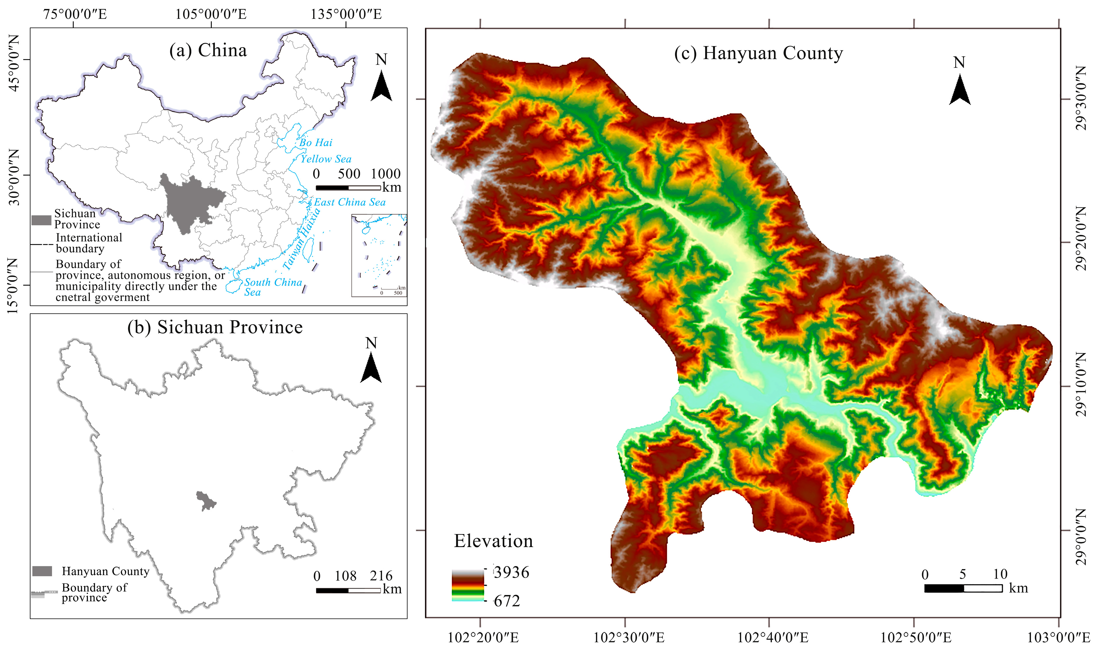
Figure 1. Location of the study area.
Land 14 02346 g001
Figure 2. POI sample points.
Land 14 02346 g002
Figure 3. Distribution and change in landscape types for agritourism in Hanyuan County.
Land 14 02346 g003
Figure 4. Changes in the four agritourism landscape types across the two study periods. Abbreviations are consistent with Figure 3: POL (production-oriented landscape), LOL (living-oriented landscape), EOL (ecological-oriented landscape), DPL (development-potential landscape). The legend “X to Y” denotes a transition from landscape type X to type Y, while “X Unchanged” indicates areas that remained as type X throughout the study period.
Land 14 02346 g004
Figure 5. Characterization of terrain gradients across landscape types.
Land 14 02346 g005
Table 1. Agritourism landscape types in Hanyuan County.
TypeCodeDominant FunctionRepresentative Land UseExample of Satellite Remote Sensing ImageEnvironmental Example
Production-oriented landscapesPOLsProduction functionDry land, paddy land, watered land, land for agricultural facilities, orchards, tea plantations and other gardens, etc.Land 14 02346 i001Land 14 02346 i002
Living-oriented landscapesLOLsLiving functionTown sites, rural settlement sites, transportation road sitesLand 14 02346 i003Land 14 02346 i004
Ecological-oriented landscapesEOLsEcological functionForested land, shrubland, other forested land, natural pasture and other grasslands, etc.Land 14 02346 i005Land 14 02346 i006
lake, river, inland mudflats, artificial reservoirs, ditches, and land for water facilitiesLand 14 02346 i007Land 14 02346 i008
Development-potential landscapesDPLsMultifunctional potentialSand, bare ground, and other landLand 14 02346 i009Land 14 02346 i010
Table 2. Metadata of auxiliary datasets.
CategorySpecificationSourceUsage
DEM30 mGeospatial Data Cloud platform of the Chinese Academy of Sciences: https://www.gscloud.cn/, accessed on 10 August 2020Terrain zoning (Section 2.3.1)
Meteorological data (temperature and precipitation)1 kmInstitute of
Tibetan Plateau Research Chinese Academy of Science:
https://data.tpdc.ac.cn/home, accessed on 4 January 2024
Driving factors analysis (Section 2.3.2)
Road networkVectorOpenStreetMap (OSM):
https://www.openstreetmap.org/, accessed on 6 March 2024
Socioeconomic indicatorsCounty-levelPeople’s Government of Hanyuan County
Ya’an Bureau of Statistics
Field research information
Table 3. Terrain gradient classification and the areal proportion of each terrain gradient.
Terrain GradientTNIAreal Proportion/%
10.22~0.412.18
20.41~0.533.94
30.53~0.6034.30
40.60~0.6546.98
50.66~0.7912.60
Table 4. List of the driver factors considered.
CategoryIndicatorVariableUnit
SocioeconomicPopulation densityX1person/km2
Farmers’ per capita net incomeX2CNY
Year-end cultivated land areaX3%
LocationDistance to nearest roadX4m
Distance to township centerX5m
TourismDistance to dining/lodgingX6m
Distance to scenic spotsX7m
Distance to water bodiesX8m
ClimateAnnual mean temperatureX9°C
Annual mean precipitationX10mm
TerrainElevationX11m
SlopeX12°
Table 5. Landscape dynamic degree from 2013 to 2023.
Type2013–20182018–2023
POL−0.32403.6637
LOL1.10312.3467
EOL0.0002−0.0027
DPL0.0770−4.9627
Table 6. Percentage transition matrix of landscape types (2013–2018).
Time 2018
TypePOLLOLEOLDPL
2013POL65.09%6.43%24.72%3.76%
LOL32.84%48.23%15.60%3.33%
EOL4.94%0.68%92.22%2.16%
DPL22.91%5.09%47.30%24.70%
Table 7. Percentage transition matrix of landscape types (2018–2023).
Time 2023
TypePOLLOLEOLDPL
2018POL80.28%8.05%9.89%1.78%
LOL18.74%70.89%8.29%2.08%
EOL6.78%1.96%90.00%1.26%
DPL37.65%6.39%27.32%28.64%
Table 8. Factors associated with production-oriented landscape changes from regression analysis (p < 0.05).
PeriodHomsmer–Lemeshow (HL)Area Under ROC CurveIndependent VariableRegression Coefficient (β)Standard Error (SE)Statistics (Wald)Significance (Sig)Incidence Rate (Exp)
2013–20180.4030.762Distance to township center (X5)−0.4530.2064.8190.0280.636
Distance to dining/lodging (X6)−1.0340.25516.4000.0000.356
Annual mean temperature (X9)0.8250.3107.1000.0082.283
Annual mean precipitation (X10)−0.6070.2565.6430.0180.545
2018–20230.6690.668Year-end cultivated land area (X3)0.2610.1274.2260.0401.298
Distance to nearest road (X4)0.3670.1406.8190.0091.443
Distance to township center (X5)−0.4670.1509.7560.0020.627
Annual mean precipitation (X10)0.2980.1503.9600.0471.348
Slope (X12)−0.2140.1093.8610.0490.807
Table 9. Factors associated with living-oriented landscape changes from regression analysis (p < 0.05).
PeriodHomsmer–Lemeshow (HL)Area Under ROC CurveIndependent VariableRegression Coefficient (β)Standard Error (SE)Statistics (Wald)Significance (Sig)Incidence Rate (Exp)
2013–20180.6350.733Year-end cultivated land area (X3)−0.4110.1527.3120.0070.663
Distance to nearest road (X4)−0.4260.1974.6840.0300.653
Distance to township center (X5)−0.4320.1726.3120.0120.650
Distance to scenic spots (X7)0.3850.1476.8830.0091.469
Annual mean temperature (X9)0.6620.2974.9790.0261.938
Slope (X12)−0.5210.12417.6760.0000.594
2018–20230.0520.666Population density (X1)0.2370.1164.2230.0401.268
Distance to nearest township center (X5)−0.2860.1424.0730.0440.751
Annual mean precipitation (X10)−0.3180.1484.6130.0320.727
Slope (X12)−0.4320.11813.5280.0000.282
Table 10. Factors associated with ecological-oriented landscape changes from regression analysis (p < 0.05).
PeriodHomsmer–Lemeshow (HL)Area Under ROC CurveIndependent VariableRegression Coefficient (β)Standard Error (SE)Statistics (Wald)Significance (Sig)Incidence Rate (Exp)
2013–20180.2270.759Distance to nearest road (X4)0.4220.1855.1790.0231.525
Annual mean precipitation (X10)−0.6450.2159.0020.0030.524
2018–20230.0760.612Distance to township center (X5)0.3460.1119.6570.0021.414
Distance to scenic spots (X7)−0.3240.1445.0540.0250.723
Table 11. Factors associated with development-potential landscape changes from regression analysis (p < 0.05).
PeriodHomsmer–Lemeshow (HL)Area Under ROC CurveIndependent VariableRegression Coefficient (β)Standard Error (SE)Statistics (Wald)Significance (Sig)Incidence Rate (Exp)
2013–20180.6340.744Distance to township center (X5)0.3900.1299.1050.0031.447
Distance to dining/lodging (X6)0.4660.14610.1740.0011.594
Annual mean temperature (X9)−0.7900.20914.3530.0000.454
Annual mean precipitation (X10)0.9390.21918.3370.0002.556
Slope (X12)0.2700.1096.1700.0131.311
2018–20230.4920.676Distance to water bodies (X8)0.3170.1118.1930.0041.372
Slope (X12)0.4690.10420.1240.0000.325
Disclaimer/Publisher’s Note: The statements, opinions and data contained in all publications are solely those of the individual author(s) and contributor(s) and not of MDPI and/or the editor(s). MDPI and/or the editor(s) disclaim responsibility for any injury to people or property resulting from any ideas, methods, instructions or products referred to in the content.