Article

Modeling Spatiotemporal Dynamics and Driving Mechanisms of Ecosystem Services Bundles in Resource-Based Cities: Supply–Demand Mismatch in Xingtai, China

1
School of Land Science and Technology, China University of Geosciences, Beijing 100083, China
2
Technology Innovation Center for Ecological Conservation and Restoration in Dongting Lake Basin, Ministry of Natural Resources, Changsha 410029, China
3
Real Estate Registration Center, Ministry of Natural Resources, Beijing 100034, China
*
Author to whom correspondence should be addressed.
These authors contributed equally to this work.
Land 2025, 14(11), 2270; https://doi.org/10.3390/land14112270
Submission received: 13 September 2025 / Revised: 2 November 2025 / Accepted: 12 November 2025 / Published: 17 November 2025

Abstract

The sustainable development of resource-based cities faces challenges due to the imbalance between ecosystem service supply and demand. This study examines Xingtai, a typical resource-based city located in northern China, using ecosystem service bundle theory to analyze the supply–demand relationships of six ecosystem services—water yield, soil retention, habitat quality, urban cooling, PM2.5 removal, and carbon sequestration—from 2000 to 2020. Based on the ratio of supply–demand, we identify ecosystem service bundles and explore their driving factors using redundancy analysis (RDA) and the geographically and temporally weighted regression (GTWR) model. Results show a clear “mountain–plain” supply gradient, with high supply in the western Taihang Mountains and low supply in urbanized eastern plains. Demand follows a “center-high, periphery-low” pattern, with urban centers showing higher demand for urban cooling and PM2.5 removal. A severe supply–demand imbalance exists: soil retention, PM2.5 removal, habitat quality, and carbon sequestration are undersupplied in urbanized areas, while water yield and urban cooling are oversupplied in the western mountains. Natural factors (precipitation and temperature) shape western mountain supply, while human activities (GDP and nighttime light) drive demand polarization in the east. GTWR results reveal that urban GDP growth and land expansion intensify demand, while stable supply in mountain areas relies on precipitation and forest cover. This study provides scientific support for the sustainable development of resource-based cities.

1. Introduction

The extraction and processing of natural resources are the core industries of resource-based cities, playing a crucial role in regional economic growth and social prosperity throughout history [1,2]. However, rapid industrialization, urbanization, and agricultural development have significantly impacted the regional ecosystem, affecting the supply and demand of ecosystem services (ESs). With drastic land cover changes, resource-based cities often face a range of ecological challenges, including environmental pollution, land degradation, and geological disasters [3]. These issues not only pose major obstacles to sustainable socio-economic advancement but also accelerate the depletion of natural resources and negatively affect ecosystem functions, particularly contributing to a decline in ecosystem services. This threatens ecosystem stability and adversely impacts human well-being [4]. Therefore, systematically studying ecosystem characteristics of resource-based cities holds significant theoretical and practical importance for optimizing land use patterns, enhancing ecosystem service capacity, and promoting urban sustainability [5].
Ecosystem services, whether directly or indirectly, provide a variety of material and non-material benefits that support human production activities and daily life, contributing fundamentally to human well-being [6]. The supply of ecosystem services refers to the products and services generated by ecosystems for human use, whereas demand represents the consumption and utilization of these products and services by humans. Together, they represent a dynamic interaction where ecosystem services are transferred from ecological systems to human societies [7]. The balance between ecosystem service supply and demand is a key component of regional sustainable development theory and is essential for understanding the interactions between human society and the natural environment [8]. In recent years, supply–demand relationships have become a focal point in international ecosystem service research, evolving from defining supply and demand concepts and refining research frameworks to focusing on the quantification and assessment of ecosystem service supply [9]. The focus has gradually transitioned towards evaluating supply–demand balance, spatial patterns, supply–demand matching relationships, and their dynamic changes. Various methods, including ecological modeling, public participation, and value assessment, have been proposed to support the quantification and spatialization of ecosystem services [10,11,12]. Additionally, ecosystem service flows, representing services that are actually utilized, serve as a critical link between supply and demand. Quantifying and assessing these flows can reveal the degree of matching between ecosystem service supply and demand [13]. Recent studies advance urban ES research. Urban ESs enhance city resilience, guiding our focus on Xingtai’s supply–demand dynamics. ES bundle frameworks inform spatial planning, supporting our clustering of distinct service patterns. Socio-ecological interactions in urban contexts underpin our GTWR analysis of drivers like urbanization. These works contextualize our high-resolution analysis, addressing resource-based city challenges [14,15,16].
The concept of ecosystem service bundles was introduced by Kareiva et al., referring to the frequent co-occurrence of multiple ecosystem service types within a specific spatiotemporal range. It is widely used to identify dominant regional ecosystem services [17,18]. In recent years, academics worldwide have increasingly explored the relationships among ecosystem services in terms of service bundles. Methods for identifying ecosystem service bundles mainly include principal component analysis (PCA), spatial autocorrelation analysis, cluster analysis, and unsupervised neural networks [19,20,21]. For example, Song used a self-organizing network approach to examine interactions among multiple ecosystem services in Fuzhou, revealing five distinct service bundles with significant spatial heterogeneity. Similarly, Z et al. applied the K-means algorithm to cluster the ecosystem service combinations of different streets in Shenzhen, identifying six ecosystem service bundle types and their dominant spatiotemporal evolution trajectories. Furthermore, researchers have explored ecosystem service bundles across various spatial scales, such as the national level, watershed scale, geographical units, and administrative units [22,23,24]. Ecosystem services bundles group co-occurring services shaped by socio-ecological drivers, revealing spatial patterns. This framework guides our study to map Xingtai’s ES bundles and analyze supply–demand mismatches [25]. However, most studies remain focused on large-scale or macro-level analyses, with fewer investigations at smaller, localized scales. There is still a lack of refined identification of different bundles and comprehensive analysis of their driving factors at the regional level.
Within the coupled dynamics of natural and human-driven processes, ecosystem services undergo significant spatiotemporal changes. Some scholars have investigated the mechanisms by which external factors—such as land use change, resource exploitation, and pollution emissions—affect ecosystem services [26,27]. Methods for exploring influencing factors include redundancy analysis (RDA), principal component analysis (PCA), regression analysis, and machine learning techniques. However, these methods have limitations when handling complex, multi-factor drivers. They often lack causal relationship analysis, fail to effectively capture interactions between variables, and overlook spatial heterogeneity. Additionally, many rely on linear assumptions or specific data distribution characteristics, making them less suitable for addressing the nonlinear and spatially dynamic nature of ecosystem services. The geographically and temporally weighted regression (GTWR) model incorporates the temporal dimension, enabling a systematic analysis of driving factors under spatiotemporal variations. It provides a powerful tool for addressing spatiotemporal no stationarity. As an emerging spatial statistical method, GTWR has been widely applied in ecosystem service valuation, vegetation protection, and urbanization studies [28,29,30].
Current research on ecological issues of resource-based cities predominantly adopts engineering and technological perspectives, utilizing physicochemical methods to restore ecological elements such as soil and vegetation [31]. However, few studies have conducted comprehensive assessments of resource-based urban ecosystems at regional scales, and even fewer have integrated both supply and demand aspects of ecosystem services to analyze social-ecological system coupling [32]. Addressing this gap, this research quantifies the supply, demand, and supply–demand ratios of six key ecosystem services (carbon sequestration, PM2.5 removal, water yield, soil retention, habitat quality, and urban cooling) in Xingtai City for 2000, 2010, and 2020 by integrating land use data and socioeconomic statistics. This study identifies spatiotemporal variations in ecosystem service supply–demand relationships and spatial matching characteristics. The self-organizing feature map (SOFM) method is employed to identify ecosystem service bundles and explore spatiotemporal patterns of multiple ecosystem service interactions. Redundancy analysis reveals differences in ecological service supply–demand across bundles and their driving mechanisms, while the GTWR model investigates the impact of socioeconomic development on ecological changes. By integrating InVEST, SOFM, and GTWR, we uncover context-specific patterns and drivers, filling a gap in applying ES bundle theory to such cities. This approach provides novel insights for urban ecological planning, addressing unique challenges like resource depletion and pollution.

2. Materials and Methods

2.1. Study Area

Xingtai City is situated in the southern Hebei Province (Figure 1), spanning between 113°45′ and 115°55′ E and 36°45′–37°55′ N. The city administers 4 districts, 12 counties, and 2 county-level municipalities, covering a total area of 12,457 km2 dominated by dryland, woodland, and construction land, with a permanent population of 7 million. Its terrain comprises two major geomorphic units: mountainous regions in the west and plains in the east. The western mountainous and hilly area occupies 3545 km2, accounting for 28% of the city’s total area, while the eastern plains cover 72% without distinct transitional zones. As a typical warm–temperate continental monsoon climate zone, the city receives 500–600 mm of annual precipitation, rendering its water resources comparatively scarce. Xingtai boasts abundant natural resources, particularly coal, iron, steel, and mineral reserves, which have significantly supported its industrial infrastructure development and energy security, establishing it as a key resource-based city in the Hebei Province and North China. However, the city increasingly faces severe resource depletion, ecological degradation, and major challenges in industrial restructuring and ecological restoration.

2.2. Spatiotemporal Changes in Ecosystem Service Supply and Demand

2.2.1. Land Use Change

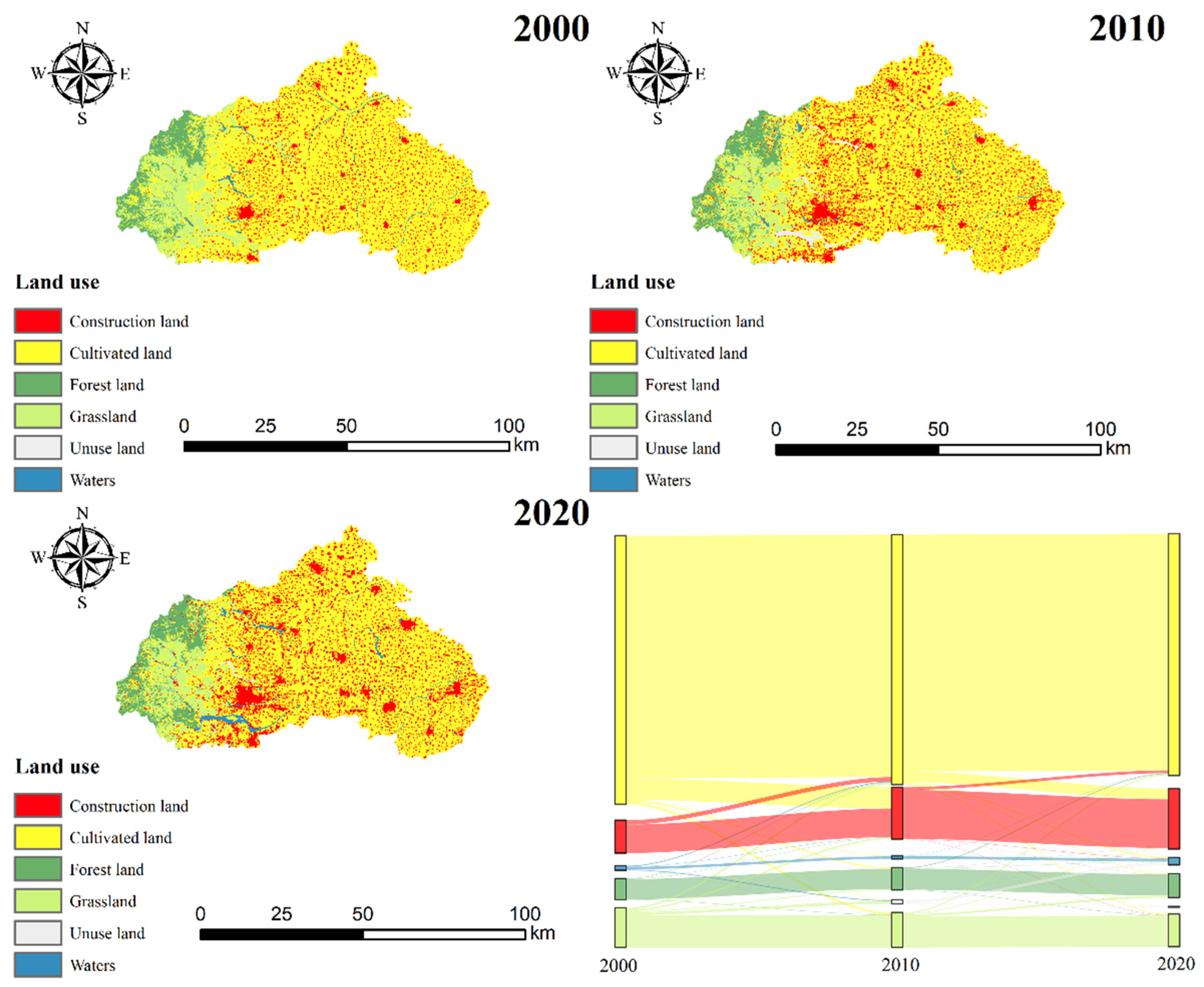
Land use data for 2000, 2010, and 2020 were acquired from the 1:100,000 scale dataset provided by the Data Center for Resources and Environmental Sciences, Chinese Academy of Sciences. A land use classification system was established based on the study area’s characteristics, categorizing land into seven types: cropland, woodland, grassland, water bodies, construction land (primarily urbanized landscapes and industrial/mining land uses), and unused land. By calculating the differences between the 2000–2010 and 2010–2020 datasets, land use transition matrices and Sankey diagrams were generated to visualize changes in land use types over time.

2.2.2. Modeling Ecosystem Services Supply and Demand

Considering the distinctive attributes of resource-dependent urban centers in the study area—existing ecological issues, data availability, and methodological feasibility—six ecosystem services were selected as representative ESs for this region. These include water yield (WY), soil retention (SR), habitat quality (HQ), urban cooling (UC), PM2.5 removal (PM2.5), and carbon sequestration (CS) which utilize Net Primary Production (NPP) as a proxy. The study conducted quantification and mapping of both the supply and demand aspects of these ecosystem services (Table 1). The selected ES focuses on provisioning and regulating categories, which are most pertinent to ecological pressures in resource-based cities (e.g., pollution and resource extraction). Cultural services, such as recreation and esthetics, were not included due to data quantification challenges and the study’s emphasis on biophysical dynamics, though they merit future investigation for a holistic urban sustainability assessment.
In this study, ecosystem service demand is conceptualized as pressure-based demand, which reflects the degree to which ecological functions are required to offset human environmental stress, rather than direct consumption or economic valuation. Population density and nighttime light intensity are therefore used as indicators of human exposure and anthropogenic pressure. This approach is consistent with recent research in ecosystem service demand modeling, where demand is defined by the spatial mismatch between ecological capacity and human stress rather than by market-based or consumption-based metrics. Nonetheless, we acknowledge that these proxy indicators provide an indirect approximation, and future research could incorporate air quality monitoring data, health exposure assessments, and policy threshold benchmarks to improve demand estimation accuracy.

2.3. Analysis of Supply–Demand Balance Relationships

2.3.1. Supply–Demand Matching

Imbalanced ecosystem service (ES) supply and demand leads to resource underutilization. This study quantifies four ES types using the Ecosystem Service Supply–demand Ratio (ESDR), integrating regional supply and demand data to identify mismatches.
E S D R = S D S m a x + D m a x / 2
where ESDR is the supply–demand ratio in the study unit; S is the actual ES supply; D is the actual ES demand; S_max is the maximum ES supply; and D_max is the maximum ES demand.

2.3.2. Composite Supply–Demand Ratio

The Composite Ecosystem Service Supply–demand Ratio (CESDR) indicates the aggregate balance between provisioning capacity and utilization requirements across multiple ecosystem services, calculated as the arithmetic mean of six selected ESDRs:
C E S D R j = 1 n i = 1 n E S D R i j
where C E S D R j denotes the ratio in grid unit j , n is the number of ES types, and E S D R i j represents the supply–demand ratio of ES type i in grid j. Both the CESDR and individual ESDR are indices highlighting spatial correspondence between high demand and low supply areas, and vice versa. In the results, zero values signify supply–demand equilibrium; positive/negative values denote surplus/deficit, respectively.

2.4. Ecosystem Service Supply–Demand Clusters

The study area, geographically positioned at the transition between the North China Plain and Taihang Mountains, exhibits complex terrain and diverse ecological challenges. Cluster analysis of ES supply–demand relationships quantifies their spatial heterogeneity. Using Kohonen’s Self-Organizing Map (SOFM), 30 m × 30 m grid units were encoded as n × 18 input vectors (n = total grids) comprising standardized ES supply, demand, and ratio metrics (min–max normalization applied) [37]. A 5 × 5 output grid (25 potential clusters) was selected via the Davies–Bouldin Index and Silhouette Coefficient validation. Training parameters: 2000 iterations (1000 coarse/fine-tuning phases), initial learning rate 0.5 (exponential decay, factor 0.95), Gaussian kernel with linearly shrinking neighborhood radius. Four dominant clusters were identified, spatially mapped via MATLAB R2019b’s selforgmap (Neural Network Toolbox).

2.5. Driving Force Analysis

2.5.1. Redundancy Analysis

To identify key factors influencing ES supply–demand dynamics, this study quantifies the explanatory power of socio-ecological drivers on cluster variations. Thirteen indicators were selected across social-ecological dimensions (Table 2) for redundancy analysis (RDA), balancing case study comparability and data feasibility.

2.5.2. GTWR Model

This study employs the geographically and temporally weighted regression (GTWR) model to analyze spatiotemporal heterogeneity and geographic variations in drivers. By capturing their spatiotemporal dynamics, GTWR reveals region-specific effects of driving factors on ecosystem service supply–demand patterns, enhancing precision in mapping spatial–temporal disparities.
Y i = β 0 x i , y i , t i + k = 1 β k x i , y i , t i X i k + ε i
where yi is the observed value at spatiotemporal location (xi,yi,ti); β0 is the regression constant for unit i, representing the intercept term in the GTWR model; βk is the regression parameter for the k-th independent variable at unit i, reflecting localized spatiotemporal effects; Xik is the value of the independent variable x at unit i, quantified using GTWR indicator system metrics; and ϵi is the model’s residual. The GTWR model assumes linear relationships between ES supply–demand ratios and drivers (e.g., GDP and precipitation), capturing spatiotemporal coefficient variations. It may not fully model nonlinear effects. Model reliability was ensured via multicollinearity tests (VIF < 5 for all drivers).
It should be noted that both RDA and GTWR are correlation-based approaches. They reveal the strength, direction, and spatial variability of associations between ecosystem services and their driving factors, but they do not in themselves establish deterministic causal relationships. Therefore, the interpretation of driving mechanisms in this study is grounded in established ecological theory and contextual land use knowledge, rather than inferred solely from the statistical outputs. The results should thus be understood as reflecting statistical associations and indicative influence pathways, rather than direct causation.

2.6. Data Sources and Processing

This study integrates meteorological, remote sensing, and statistical data (Table 3). All meteorological and environmental datasets underwent interpolation and spatial analysis to ensure consistency and accuracy, standardized under the WGS_1984_UTM_Zone_49N projection. Processing was implemented using ArcGIS 10.8. To ensure spatial consistency among datasets with different native resolutions (30 m, 1 km, and county-level), all raster data were resampled to a uniform grid of 1 km resolution. Continuous variables such as NDVI and precipitation were processed using bilinear interpolation, while categorical variables such as land use type were resampled using a majority filter to preserve dominant landscape features. County-level socio-economic indicators were spatially downscaled to the same resolution through area-weighted interpolation. Population and land use statistics were standardized to the 2020 administrative boundary framework to avoid distortions caused by boundary adjustments over time. Since the objective of this study is to examine relative spatial differences and temporal trends rather than absolute economic magnitudes, these harmonization steps help minimize potential bias while maintaining the validity of the long-term analysis.

3. Results

3.1. Land Use Changes

Figure 2 illustrates that the main land use types in Xingtai City, ranked by area, are cropland, construction land, grassland, forest land, water bodies, and unused land. From 2000 to 2020, the city’s land use pattern changed significantly, characterized by a decline in agricultural land, exponential growth of construction land, and a moderate increase in ecological land (e.g., forest and water bodies) (Table 4). First, cropland decreased notably, while construction land increased significantly. The proportion of cropland fell from 73.26% to 65.99%, a reduction of 906.863 km2. Construction land rose from 8.96% to 16.48%, an increase of 937.572 km2. Second, grassland areas declined overall, while forest areas grew. Grassland decreased from 10.75% to 8.80%, mainly converted to cropland (86.527 km2) and construction land (73.338 km2). Forest land increased from 5.78% to 6.50%, a gain of 87.532 km2. Third, water bodies and unused land showed different trends. Water bodies grew from 1.25% to 2.06%, increasing by 101.443 km2. Unused land expanded slightly to 21.443 km2, mostly converted to construction land.

3.2. Ecosystem Service Supply and Demand Dynamics

3.2.1. Spatial–Temporal Characteristics of Ecosystem Service Supply

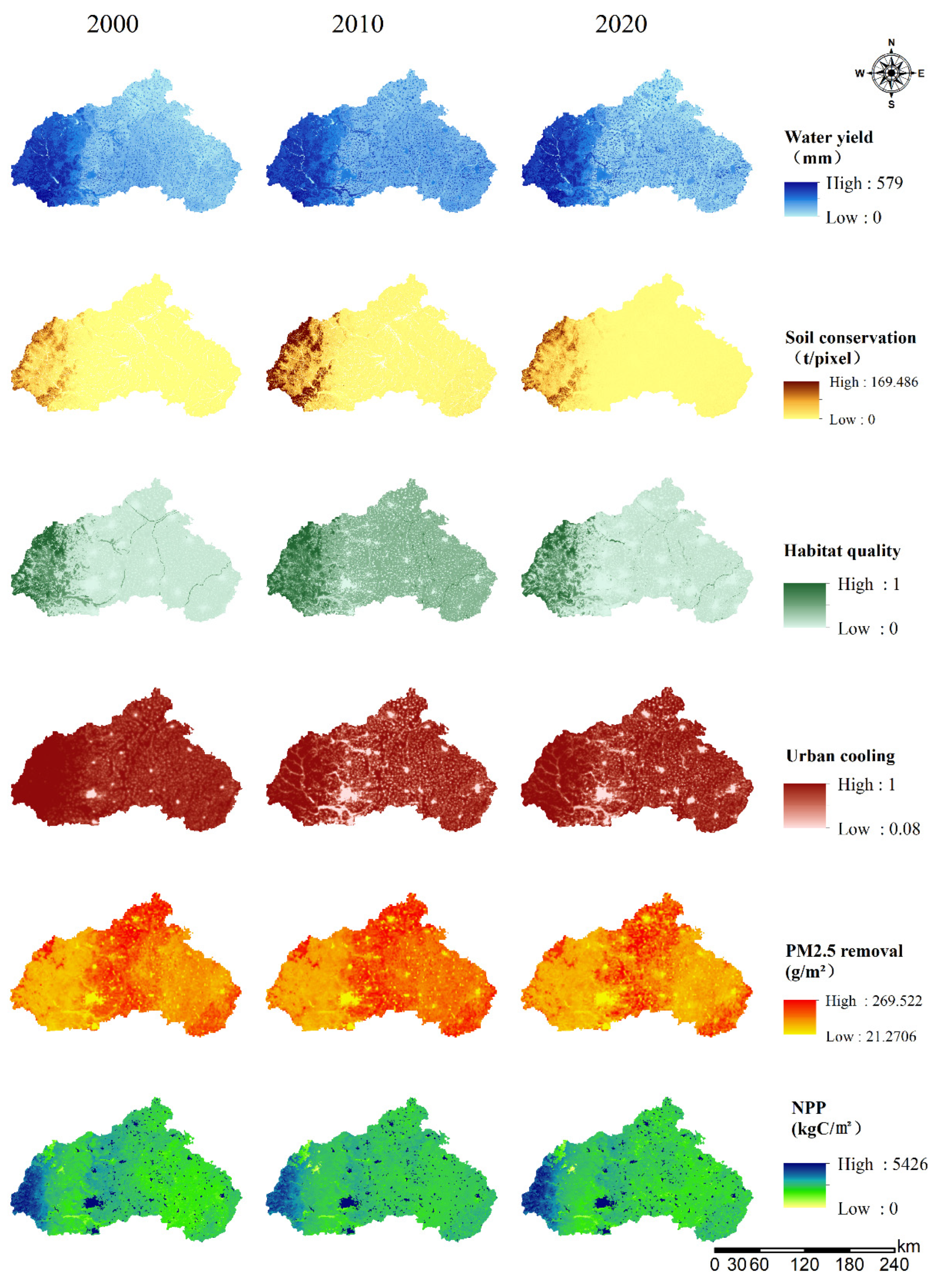
From 2000 to 2020, Xingtai City’s ecosystem services showed a distinct west–east gradient (Figure 3). The western Taihang Mountains had high water yield (peak 579 mm) and soil retention (169.486 t/pixel), linked to elevation and forest cover, while eastern plains scored low. Habitat quality was high in the west but low in urban–agricultural transition zones. Urban cooling was weakest (≤0.08) in eastern plains, correlating with construction land. PM2.5 removal peaked in western forests (269.522 g/m2) and was lowest in eastern industry (21.2706 g/m2). Carbon sequestration was highest in western forests (5426 kgC/m2). Zero-value zones expanded from 6.3% to 14.1%, tracking urbanization. Temporally, water yield >500 mm areas shrank by 12.3% post-2010; NPP high zones shifted west (2010–2020); low heat island (<0.2) and PM2.5 removal (<50 g/m2) zones grew to 20.1% and 21.3%, respectively. Soil retention varied <3%, and habitat quality remained stable, reflecting topographic and vegetative controls.

3.2.2. Spatial–Temporal Characteristics of Ecosystem Service Demand

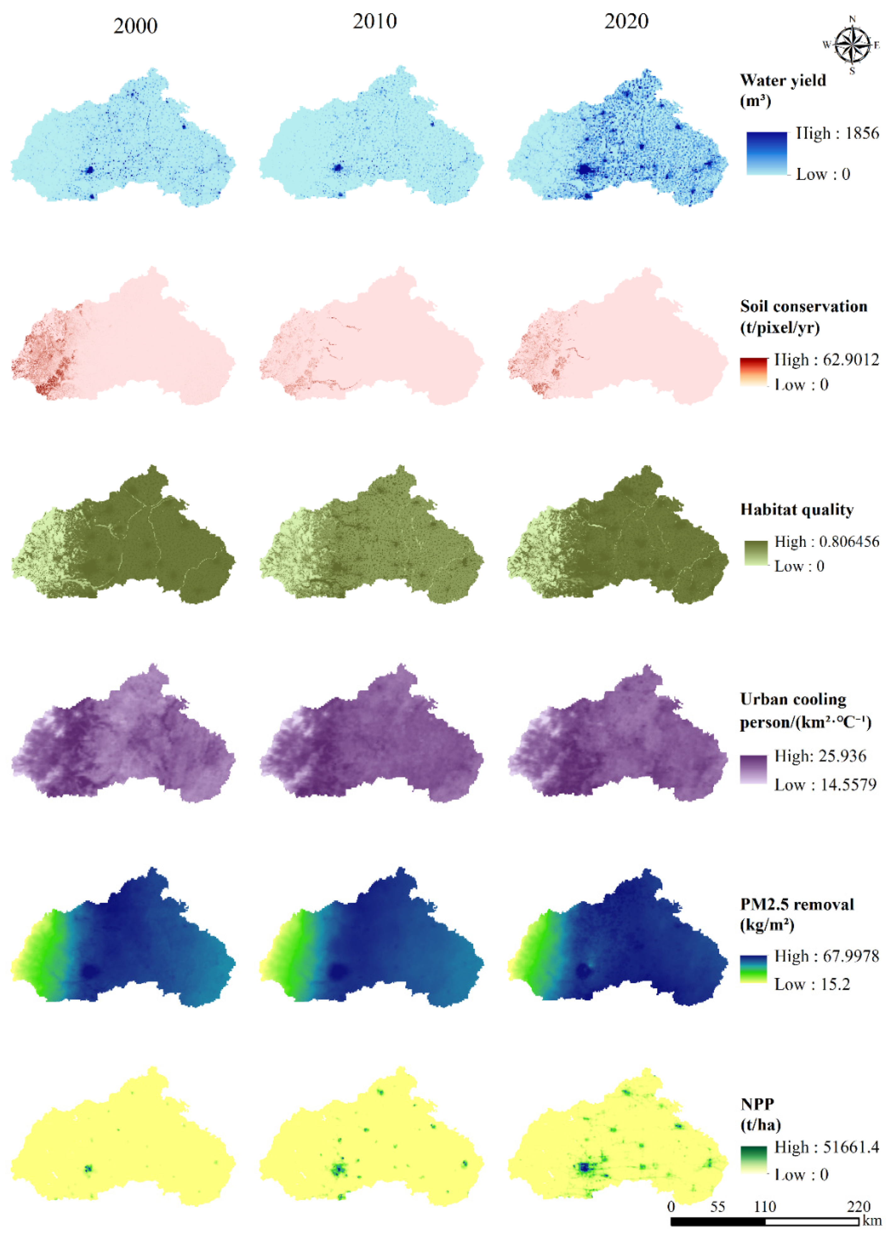
From 2000 to 2020, Xingtai’s ecosystem service demand showed a distinct west–east gradient (Figure 4). Urbanization drove the rapid expansion of high-demand zones in eastern plains for water, cooling, PM2.5 removal, and carbon sequestration, aligned with construction growth. Western mountains maintained stable low demand due to natural constraints. Soil retention demand concentrated in erosion-prone hills, slightly decreasing with cropland intensification. Habitat quality demand expanded along urban–rural edges, while cooling and PM2.5 removal demand radiated from urban centers. Urban areas saw demand intensify as follows: cooling zones grew by 1.8× (peaking at 27.1 person/(km2·°C−1)) and PM2.5 removal zones grew by 1.5× (70.5 kg/m2 peak). Carbon demand shifted outward with urban expansion, while western low-demand areas persisted, reflecting topographic controls.

3.3. Characteristics of Supply–Demand Relationships

3.3.1. Integrated Supply–Demand Ratio

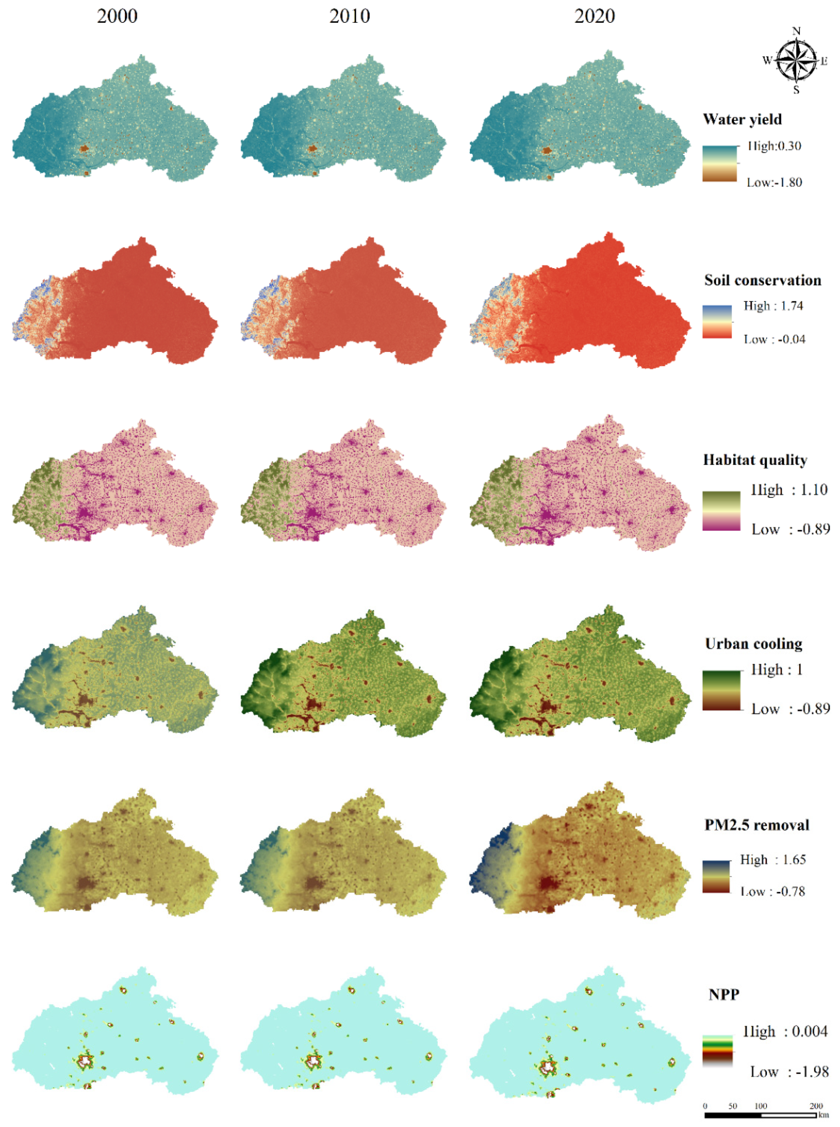
Figure 5 shows that all six ecosystem services in Xingtai from 2000 to 2020 followed a west–east gradient in supply–demand ratios—high in the mountainous west, low in the urbanized plains—reflecting both natural conditions (terrain and vegetation) and human activities (urbanization and agriculture). Urbanization-related services (urban cooling and PM2.5 removal) showed increasing spatial clustering of low-ratio zones, while nature-driven services (water yield and soil retention) saw slight shrinkage in high-ratio areas due to rainfall fluctuations. Water yield ratios ranged from 0.30 (high, in recharge zones) to −1.80 (low, in irrigation belts). Soil retention ratios peaked at 1.74 in forested hills and dropped to -0.04 in cropland plains, showing farming’s limiting effect. Habitat quality had a stark contrast (1.10 to −0.89), highlighting the gap between core protected areas and degraded zones. Urban cooling ratios (1.0 to −0.89) reflected weak regulation in urban cores, with low-ratio zones becoming more clustered. PM2.5 removal ratios (1.65 to −0.78) mirrored vegetation vs. industrial areas. Carbon sequestration (NPP) showed sharp differences (0.004 to −1.98), with low ratios expanding along urban growth zones.

3.3.2. Supply–Demand Matching Degree

The composite ecosystem service supply–demand ratio (CESDR) used in this study indicates the relative balance between estimated supply and proxy-based demand at the grid scale. A negative CESDR denotes that supply is estimated to be lower than demand in that location; however, the policy’s relevance to any given negative value depends on service-specific ecological thresholds, management objectives, and risk tolerance. To make spatial deficit mapping more actionable for planners, we adopt a pragmatic, empirically grounded classification based on the CESDR distribution in Xingtai: severe deficit (CESDR ≤ −0.50), moderate deficit (−0.50 < CESDR ≤ −0.20), mild deficit (−0.20 < CESDR < 0), balanced (0 ≤ CESDR ≤ 0.20), and surplus (CESDR > 0.20). These cutoffs are intended as prioritization guidelines, not as fixed ecological breakpoints.
Figure 6 reveals significant spatiotemporal changes in Xingtai’s composite ecosystem supply–demand ratio (CESDR) from 2000 to 2020, showing a worsening supply–demand imbalance. Balanced areas decreased from 44% (2000) to 36% (2020), while deficit zones (supply < demand) expanded from 34% to 48%, accelerating post-2010—reflecting surging demand from urbanization and agricultural expansion. Surplus zones (supply > demand) shrank from 22% to 16%, concentrated in western hills where the CESDR declined from 0.45 to 0.28 due to climate change and human pressures. Eastern plains exhibited intensifying deficits (CESDR: −0.3 to −0.45), with low-value zones spreading from urban/agricultural cores. Transitional areas shifted from near-balanced (2000) to marked deficits (CESDR < −0.3 by 2020), highlighting escalating demand surpassing supply capacities.

3.4. Spatial Variation in Ecosystem Service Bundles

3.4.1. Bundle Classification

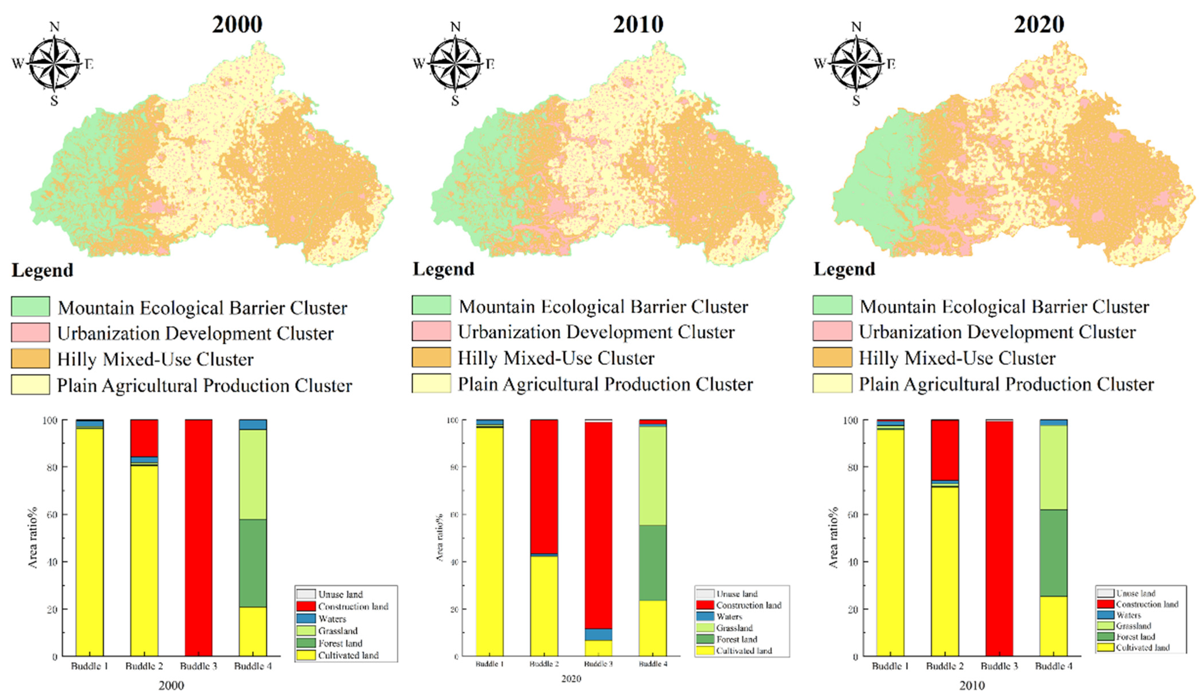
Figure 7 identifies four ecosystem service clusters in Xingtai: mountain ecological barrier (western Taihang Mountains, forest-dominated with stable structure and high water/carbon services), urban development (city periphery), hilly composite use (central/southeastern hills and mixed cropland/grassland with diversified services), and plain agricultural production (eastern plains, >85% cropland reflecting intensive farming). Spatiotemporal analysis shows stable distributions for mountain and plain clusters, while urban clusters expanded continuously with urbanization. Hilly clusters experienced cropland/grassland decline and slight construction land growth under land development pressures, highlighting urbanization-driven spatial restructuring and varied regional supply characteristics.

3.4.2. Analysis of Ecosystem Service Proportions in Each Bundle

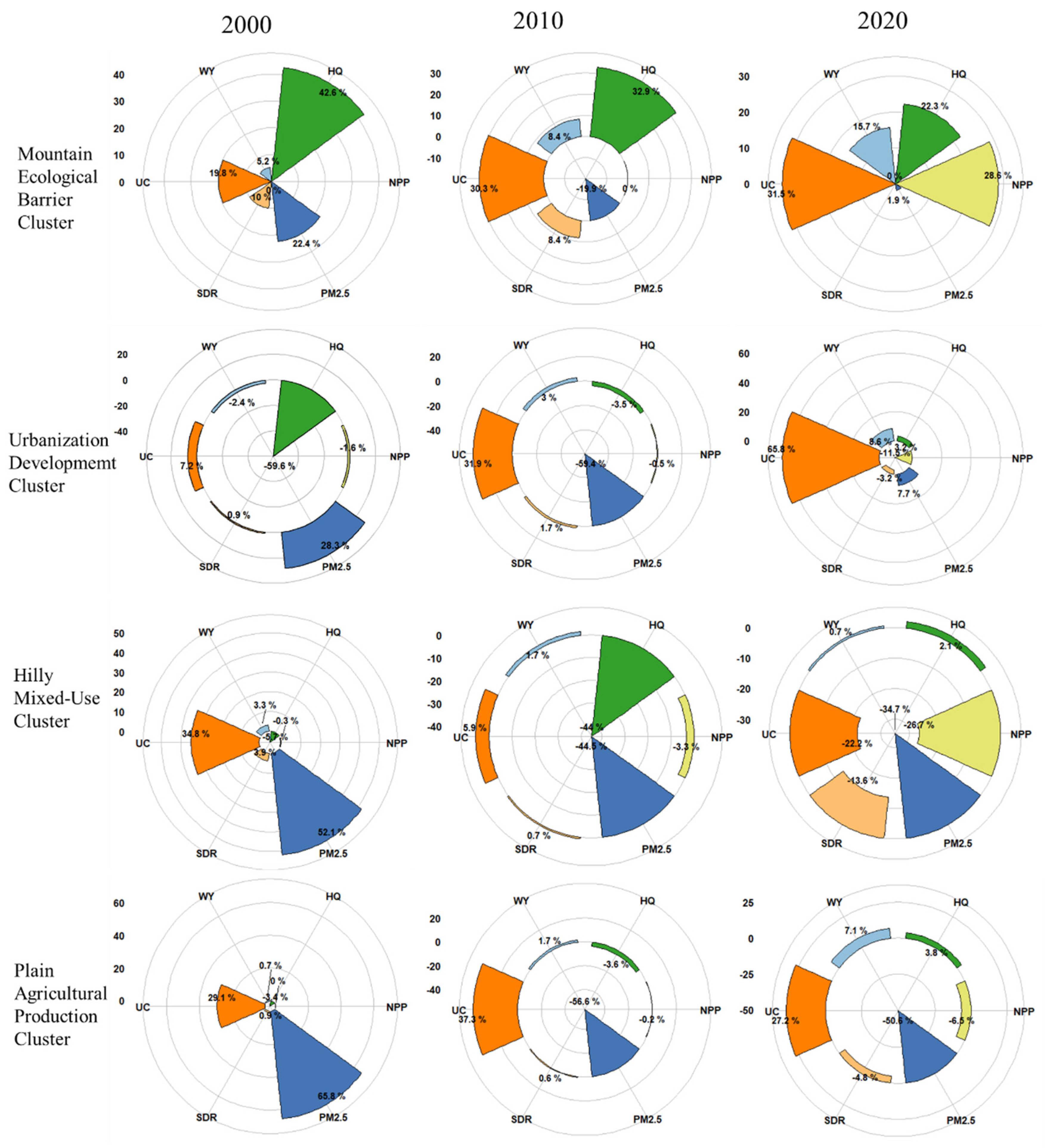
Figure 8 demonstrates that the spatiotemporal evolution of Xingtai’s four ecosystem service clusters reflects dynamic supply–demand adjustments driven by natural human activity gradients. From 2000 to 2020, mountain barrier clusters (natural dominant) maintained stability (<5% fluctuation) while plain agricultural clusters declined (>10%), highlighting contrasting trends. Western mountain clusters (core supply area) sustained high PM2.5 removal and carbon sequestration (NPP) shares (>45% average), increasing 3.2% and 2.8% post-2010, supported by forest coverage. Habitat quality (HQ) and soil retention (SR) varied <2%, confirming natural regulation stability. Eastern clusters showed human-induced degradation; urban clusters’ water yield fell from 58.6% (2000) to 52.1% (2020), SR dropped 9.1%, reflecting intensified farming impacts. Plain agricultural clusters saw urban cooling (UC) and PM2.5 removal decrease by 12.6% and 10.2% and NPP declined by 8.9%. Transitional hilly clusters achieved balance post-2010, with UC and PM2.5 removal shares rising by 4.3% and 3.7%.

3.5. Factors Influencing Ecosystem Service Supply–Demand Ratios

3.5.1. RDA

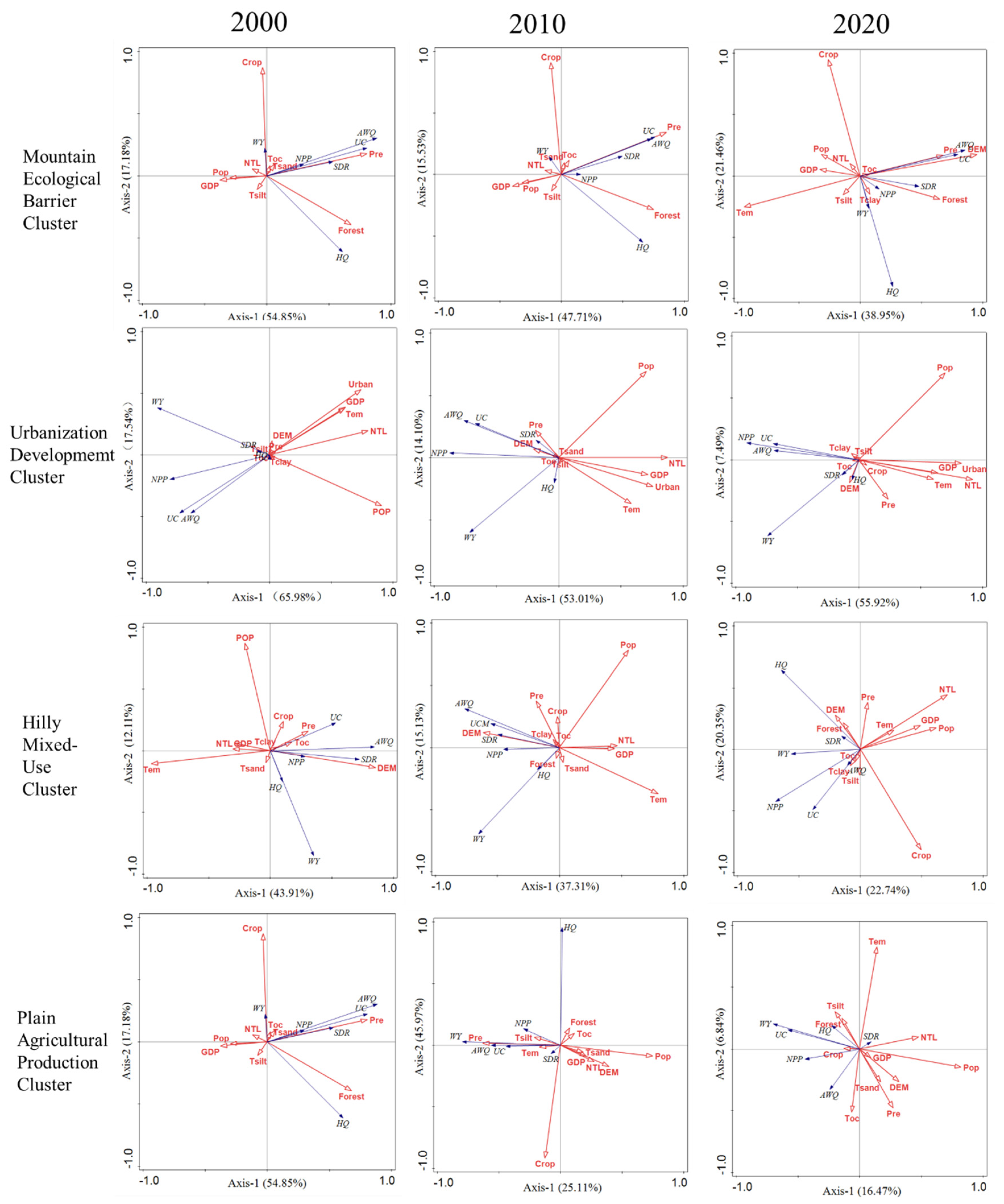
This section reveals significant spatiotemporal heterogeneity in drivers of Xingtai’s ecosystem service clusters from 2000 to 2020 via redundancy analysis (RDA), as shown in Figure 9. Key drivers remained stable, but their contributions shifted dynamically. Urban clusters showed strengthened GDP and population density influences, while natural factors dominated mountainous/hilly clusters. Mountain barrier clusters were primarily driven by forest cover (73.1% explanatory power, p < 0.024), positively affecting PM2.5 removal (PR), habitat quality (HQ), urban cooling (UC), and carbon sequestration (NPP). Precipitation governed water yield (WY) and soil retention (SR). Urban clusters relied on GDP, population density, and nighttime lights (71.4% explanation), with GDP increasingly driving UCM and NPP. Hilly clusters exhibited blended natural–social drivers (67.2% explanation), influenced by cropland, population, and temperature. Plain agricultural clusters depended on cropland area (58.4% explanation), enhancing PM2.5, NPP, SR, and HQ, while WY responded to precipitation.

3.5.2. Analysis of GTWR Model

To address multicollinearity, each explanatory variable underwent standardization and correlation testing. SPSS 26.0 software was employed to standardize both dependent and independent variable data. Multicollinearity testing was conducted on all standardized variables using regression analysis tools, with variance inflation factor (VIF) values controlled below five. Regression analysis confirmed that all selected variables passed multicollinearity testing. Using ArcGIS 10.8 software, OLS, geographically weighted regression (GWR), and spatiotemporal geographically weighted regression (GTWR) models were compared for the drivers of ecosystem service supply and demand in Xingtai City from 2000 to 2020. The fitting results for each regression model are presented in Table 5. Table 5 indicates that the coefficient of determination (R2) values, from highest to lowest, correspond to the GTWR model, GWR model, and OLS model, respectively. Similarly, the AICc values, from lowest to highest, correspond to the GTWR model, GWR model, and OLS model, respectively. Consequently, the spatiotemporal geographically weighted regression (GTWR) model demonstrates superior fitting performance.
The spatiotemporal dynamics analysis of driving factor regression coefficients based on the GTWR model indicates that the mechanisms underpinning the supply and demand of ecosystem services in Xingtai City from 2000 to 2020 exhibit significant spatial heterogeneity and temporal non-stationarity (Figure 10). Comprehensively, among natural factors, the spatial differentiation characteristics of the regression coefficients for precipitation (Pre) and temperature (Tem) are highly coupled with the geographical gradient. In the western mountainous region, the Pre coefficient (0.059–0.243) exhibits a positive driving effect, consistent with the spatial distribution of water yield demand. However, in the eastern plains, the Tem coefficient (−0.150 to 0.214) exhibited a negative inhibitory effect, overlapping with areas of expanding urban heat island mitigation demand. Among human activity factors, the negative effects of urbanization (urban: −0.300 to −0.022) and nighttime light index (NTL: −1.011 to 0.217) intensified persistently in the eastern urban core, with their high-value zones (β > 0.2) coinciding with regions of heightened PM2.5 removal and heat island regulation requirements. NTL: −1.011 to 0.217) intensified persistently in the eastern urban core. Their high-value bands (β > 0.2) aligned with the expansion trajectories of high-demand zones for PM2.5 removal and heat island regulation, indicating that urban sprawl exacerbates local environmental service pressures. The driving effects of agricultural activity (Crop) and forest cover (Forest) exhibit an east–west reversal pattern: crop coefficients (−4.557 to 0.300) demonstrate significant negative impacts (β<-2.0) in eastern farmland-dense zones, spatially linked to low soil retention demand areas; The forest coefficient (−1.210 to 0.454) exhibits a positive driving effect (β > 0.3) in forested regions of the west, supporting the natural anchoring effect for habitat quality demands. The spatiotemporal variation in regression coefficients for GDP and population (POP) is pronounced. High GDP zones (β > 0.096) exhibit a belt-like distribution along industrial corridors, expanding by 1.8-fold between 2010 and 2020—mirroring the spread of areas with zero carbon sequestration service demand. (Note: β denotes standardized regression coefficient).

4. Discussion

4.1. The Dramatic Changes in Ecosystem Service Supply–Demand in Recent Decades

The supply capacity of six ecosystem services has significantly declined due to land use changes and human-induced processes. Urban cooling weakened annually, driven by urban expansion and green space loss, aligning with findings on urbanization exacerbating heat island effects in the Beijing–Tianjin–Hebei region [38]. Habitat quality notably deteriorated in central and southern areas due to reduced ecological land. Soil retention and carbon sequestration declined sharply from cropland loss, land use shifts, and mining. Water yield capacity remained low due to water scarcity and unmet ecological demands. PM2.5 removal weakened from diminished ecosystem self-purification, reflecting limited ecological support for air quality improvement [39].
The ecosystem service demand rose markedly with socioeconomic and population growth. Urban cooling and carbon sequestration needs intensified, particularly in rapidly urbanizing areas, exacerbating supply–demand imbalances. Habitat quality demand increased with ecological awareness, yet policy efforts failed to resolve persistent gaps. Soil retention demand concentrated in plain agricultural clusters, where cropland protection conflicts with infrastructure expansion. Water yield and PM2.5 removal exhibited stark regional disparities, surging in resource-dependent cities due to water scarcity and pollution, consistent with Beijing–Tianjin–Hebei environmental pressures [40].
This study reveals significant spatial heterogeneity in ecosystem service supply–demand patterns across cluster types. Plain agricultural clusters, predominantly located in agriculturally rich areas, exhibited sustained high supply–demand ratios for water yield and soil retention. Urbanization clusters, concentrated in urban/peri-urban zones, showed severe imbalances (demand > supply) for PM2.5 removal and urban cooling, worsening over time. Hilly multifunctional clusters maintained balanced supply–demand relationships in less-developed regions [41]. Mountain ecological barrier clusters, situated in sensitive zones, demonstrated high supply ratios for habitat quality and carbon sequestration. Overall, Xingtai’s ecosystem service imbalances intensified spatiotemporally. Accelerated urbanization and land use changes from 2000 to 2020 exacerbated supply–demand conflicts, particularly in urbanization clusters, underscoring how economic growth pressures ecosystem capacities despite meeting human demands.

4.2. Ecosystem Service Supply–Demand Bundles Reflect the Spatial Heterogeneity of Ecological Functions

Natural factors exhibit relatively stable spatiotemporal distributions, predominantly influenced by topographic and climatic conditions, while the spatial patterns of human activity factors show significant dynamic changes closely aligned with urbanization processes. Spatially, the eastern plains demonstrate the highest human activity intensity, manifested through urban land expansion, population density growth, and the clustering of high nighttime light values, which markedly differ from the spatial distribution of high-value natural factors. In contrast, the western mountainous regions with high natural factor values exhibit strong ecological functional stability due to weaker human activity intensity. Changes in Xingtai’s land use patterns result from the interplay of natural forces and human influences, with their mechanisms displaying significant spatiotemporal heterogeneity. Temporally, natural factor distributions remain largely stable, serving as ecological background conditions for regional land use, whereas human activity factors exhibit distinct phased changes. From 2000 to 2020, urbanization and economic development accelerated significantly, gradually strengthening human activities’ dominant role in land use. Spatially, natural factors display a gradient decreasing from west to east, while human activity factors show pronounced spatial differentiation, with strong aggregation effects in the eastern plains and weaker interference in the western mountains [42].
Regarding natural drivers, the spatial differentiation of soil organic matter, rainfall, and surface temperature aligns closely with the literature highlighting the critical role of climatic factors and soil quality in agro-ecosystem service provisions [43,44]. Redundancy analysis (RDA) reveals significant spatial differences and dynamic variations in ecosystem service drivers across ecological clusters; mountain and hill clusters are primarily governed by natural factors, urbanization clusters by socioeconomic factors, and plain clusters by agricultural resource factors. These regional driver differences reflect the diversity of ecosystem service supply–demand patterns and establish a scientific foundation for spatially targeted ecological conservation and management approaches. Comparative analysis of GTWR coefficients indicates that these factors’ driving effects on ecological service demand significantly intensify in urbanizing regions, consistent with the conclusion that “accelerated urbanization increases ecosystem service demand” [45]. The GTWR results reveal that urbanization drives PM2.5 removal and urban cooling deficits in eastern urban clusters, while precipitation and forest cover enhance water yield in western mountains. These socio-ecological interactions explain supply–demand mismatches, with high GDP amplifying urban demand. This highlights the need for targeted green infrastructure to balance human–nature dynamics. Furthermore, RDA results highlight that the nighttime light index not only directly reflects economic activity intensity but also positively correlates with ecosystem supply–demand imbalances.
In terms of coupling effects, this study reveals that the interactions between natural conditions and human activities differ significantly across development intensity gradients. Natural factors demonstrate relatively stable influences on ecological service supply at the regional scale, whereas human activity factors exhibit stronger temporal fluctuations, particularly during periods of rapid urban expansion in resource-dependent cities. Meanwhile, it is important to acknowledge that the ecosystem service estimates in this research are derived from biophysical simulation models and publicly available datasets, which may introduce uncertainty. To ensure reliability, model outputs were cross-validated against hydrological trends, NDVI changes, and land use dynamics, and the analysis focuses on relative spatial patterns rather than absolute quantities. These findings underscore that the coupling of natural endowments and socioeconomic dynamics is the core driver of ecosystem service bundle differentiation. Therefore, ecological governance in resource-based cities should adopt differentiated management strategies; high-intensity human activity zones should prioritize land use structural optimization and ecological restoration to mitigate urbanization pressures, while ecological conservation zones should reinforce natural ecosystem stability. Future work may further enhance empirical robustness through long-term monitoring networks and high-resolution ecological data assimilation [46].

4.3. The Development and Ecological Protection of Resource-Based Cities Requires Coordinated Attention

As a typical resource-based city, the study of temporal and spatial changes in ecosystem services and their underlying drivers in Xingtai provides critical scientific evidence for regional ecological conservation and holds significant implications for the high-quality transformation of resource-dependent cities. By quantitatively assessing ecosystem service supply, demand, and their ratios, this research identifies the spatial distribution and dynamic patterns of ecosystem service bundles, offering data support for land use optimization and ecological protection strategies [47]. Based on clustering results, we propose region-specific governance strategies: (1) For mountainous ecological barriers, increase forest cover by 15% by 2035 in western Taihang Mountains to enhance water yield and carbon sequestration, prioritizing reforestation in degraded areas. (2) In urban development clusters, limit construction land expansion to 5% annually in eastern plains and achieve 25% green space coverage by 2030 to address PM2.5 removal and urban cooling deficits. (3) For hilly composite use areas, promote mixed land use planning to balance habitat quality and agriculture. (4) In plain agricultural zones, implement soil retention practices on 30% of farmland by 2030 to reduce erosion. These measures target supply–demand imbalances for sustainable development [48].
In the context of global ecosystem governance, the findings of this study align with widely used policy tools such as payments for ecosystem services (PESs), biodiversity offsetting mechanisms, ecological redline zoning, and large-scale ecological restoration programs. Recent international assessments have emphasized that effective biodiversity and ecosystem service management require not only conservation measures but also spatially differentiated strategies tailored to local socio-ecological conditions [15,49]. The ecosystem service bundle approach adopted in this study provides a framework for identifying zones where ecological protection should be prioritized and zones where controlled development and ecological compensation are more suitable. Although the empirical focus of this research is Xingtai, the governance logic is transferable to other regions—including tropical ancient forest areas in Indonesia, Colombia, Sri Lanka, and Ghana—where balancing conservation value with livelihood and developmental needs remains a central challenge. Therefore, our results offer a spatial decision-support perspective that may assist policymakers in designing adaptive, region-specific strategies for coordinated ecological protection and sustainable land use transitions.
Furthermore, the ecosystem service bundles identified in this study provide a basis for aligning ecological governance with sustainability planning in resource-dependent cities. The Mountain Ecological Barrier Bundle supports long-term ecological security and carbon storage, contributing directly to SDG 13 and SDG 15. The Urban Development Bundle highlights the need for resilient urban transformation, consistent with SDG 11 by promoting compact growth and low-impact infrastructure. The Hilly Multifunctional Transition Bundle suggests pathways for adaptive land use strategies that balance ecological conservation with livelihood needs, supporting integrated landscape management. Meanwhile, the Plain Agricultural Production Bundle indicates opportunities to transition from high-input agriculture to green production systems through ecological compensation and farmland protection policies. These bundle-specific insights provide actionable guidance for spatial planning, land use regulation, and ecological compensation schemes in resource-based cities undergoing sustainable development transitions [50].

4.4. Limitations

It is important to acknowledge several limitations of this study. First, the ecosystem service estimates are derived from biophysical simulation models and publicly available datasets, which may introduce uncertainty. Although parameter settings for water yield, soil retention, and PM2.5 removal were based on regionally calibrated coefficients, and model outputs were cross-validated using observed hydrological trends, NDVI dynamics, and land use change patterns, field-based validation was not feasible at the regional scale. Additionally, ecosystem services quantified using the InVEST model and remote sensing indicators may be subject to over- or under-estimation in regions with dense vegetation or homogeneous land cover, which could obscure fine-scale spatial and temporal heterogeneity. Second, while this study focuses on relative spatial patterns rather than absolute magnitudes to minimize uncertainty, the explanatory models still rely on simplifying assumptions. The GTWR framework assumes primarily linear relationships between ecosystem services and human activities, and does not explicitly incorporate spatial spillover effects, climatic variability, or policy-driven changes. Moreover, although the analysis identifies key biophysical and socio-economic drivers, further work is needed to quantitatively assess the contribution of each driver and to integrate additional influential factors. Future research should enhance empirical reliability and model robustness by incorporating long-term field monitoring networks, higher-resolution data assimilation, nonlinear or causal inference modeling approaches, and a broader range of socioeconomic and policy variables [51].

5. Conclusions

This study conducted a comprehensive assessment of the supply and demand of six ecosystem services (ESs) in Xingtai City. Based on the Ecosystem Service Bundles (ESBs) framework. ES supply–demand clusters were identified and analyzed through RDA and GTWR to explore their driving factors and propose targeted planning recommendations. The principal conclusions can be summarized as follows: (1) All six ES types demonstrate marked spatial variability. High supply values are disproportionately located in the western mountainous areas, while low values dominate the eastern plains. In contrast, demand is highest in urban and county centers, decreasing outward. (2) Although the overall supply–demand ratios are relatively balanced, spatial mismatches are pronounced. Soil retention, PM2.5 removal, habitat quality, and NPP are in a state of undersupply, with supply–demand ratios of −0.04, −0.13, −0.56, and −0.28, respectively. Water yield and urban cooling show slight oversupply, with ratios of 0.017 and 0.008. Spatially, supply–demand mismatches are concentrated in urban centers, while peripheral areas tend to have surplus supply. (3) Supply–demand clusters were delineated according to ratio metrics and their drivers were analyzed accordingly. Natural factors (e.g., precipitation and temperature) anchor supply capacity through geographic gradients, while human activity factors (e.g., GDP and NTL) drive demand polarization in a “center–periphery” pattern. The GTWR model indicates that GDP growth and urban expansion are significantly correlated in urban development clusters, while service stability in mountainous ecological barrier clusters is positively influenced by precipitation and forest cover.
Based on the identified bundle patterns, this study recommends differentiated and cluster-based governance strategies rather than adopting uniform measures across the entire region. In the western mountainous areas, which function as ecological barrier clusters, maintaining ecological stability should be prioritized by reinforcing ecological protection controls and preventing further land use conversion. In contrast, the eastern urban development pressure clusters require the guidance of compact and intensive urban growth while strengthening ecological function zoning to alleviate concentrated ecosystem service demand pressures. For the agricultural production clusters located in the central plains, improving land management practices and enhancing vegetation cover are essential to mitigate the decline in ecosystem service supply associated with intensive agricultural activities. Additionally, in the river–wetland regulation corridor, ecological connectivity should be enhanced to ensure the continuous flow and coordination of ecosystem services across landscape units. These differentiated strategies emphasize spatially adaptive governance aligned with the ecosystem service characteristics of each cluster.
Our study contributes to ES bundle theory by applying it to a resource-based city, revealing four distinct bundles and their spatially heterogeneous drivers via GTWR. Unlike standard applications, this high-resolution analysis (30 m × 30 m) offers novel insights into managing supply–demand imbalances in urbanizing, resource-scarce contexts. These findings inform targeted ecological restoration, advancing sustainable planning in similar cities globally.

Author Contributions

Conceptualization, Z.W.; methodology, Z.W.; software, K.L. and Q.H.; validation, K.L. and C.Y.; formal analysis, R.W.; investigation, K.L.; data curation, R.W.; writing—original draft preparation, R.W.; writing—review and editing, K.L., Q.H., L.X., Z.W., C.Y. and M.X.; supervision, Z.W.; project administration, Q.H. and M.X.; funding acquisition, L.X. All authors have read and agreed to the published version of the manuscript.

Funding

This study was supported by the National Natural Science Foundation of China (Project NO.: 42207530), Hunan Provincial Natural Science Foundation (Project NO.: 2024JJ8320), and Fundamental Research Funds for the Central Universities (Project NO.: 292022004).

Data Availability Statement

The datasets analyzed during the current study are available from the corresponding author upon reasonable request.

Conflicts of Interest

The authors declare no conflicts of interest.

References

  1. Wang, Q.; Liu, M.; Tian, S.; Yuan, X.; Ma, Q.; Hao, H. Evaluation and Improvement Path of Ecosystem Health for Resource-Based City: A Case Study in China. Ecol. Indic. 2021, 128, 107852. [Google Scholar] [CrossRef]
  2. Zhu, S.; Huang, J.; Zhao, Y. Coupling Coordination Analysis of Ecosystem Services and Urban Development of Resource-Based Cities: A Case Study of Tangshan City. Ecol. Indic. 2022, 136, 108706. [Google Scholar] [CrossRef]
  3. Li, S.; Zhao, Y.; Xiao, W.; Yue, W.; Wu, T. Optimizing Ecological Security Pattern in the Coal Resource-Based City: A Case Study in Shuozhou City, China. Ecol. Indic. 2021, 130, 108026. [Google Scholar] [CrossRef]
  4. Costanza, R. Ecosystem Services: Multiple Classification Systems Are Needed. Biol. Conserv. 2008, 141, 350–352. [Google Scholar] [CrossRef]
  5. Shi, T.; Yang, S.; Zhang, W.; Zhou, Q. Coupling Coordination Degree Measurement and Spatiotemporal Heterogeneity between Economic Development and Ecological Environment—Empirical Evidence from Tropical and Subtropical Regions of China. J. Clean. Prod. 2020, 244, 118739. [Google Scholar] [CrossRef]
  6. Boyd, J.; Banzhaf, S. What Are Ecosystem Services? The Need for Standardized Environmental Accounting Units. Ecol. Econ. 2007, 63, 616–626. [Google Scholar] [CrossRef]
  7. Fan, S.; Yan, M.; Yu, L.; Chen, B.; Zhang, L. Integrating Ecosystem Service Supply–Demand and Ecological Risk Assessment for Urban Planning: A Case Study in Beijing, China. Ecol. Indic. 2024, 161, 111950. [Google Scholar] [CrossRef]
  8. You, C.; Qu, H.; Wang, C.; Feng, C.-C.; Guo, L. Trade-off and Synergistic of Ecosystem Services Supply and Demand Based on Socio-Ecological System (SES) in Typical Hilly Regions of South China. Ecol. Indic. 2024, 160, 111749. [Google Scholar] [CrossRef]
  9. Jones, L.; Norton, L.; Austin, Z.; Browne, A.L.; Donovan, D.; Emmett, B.A.; Grabowski, Z.J.; Howard, D.C.; Jones, J.P.G.; Kenter, J.O.; et al. Stocks and Flows of Natural and Human-Derived Capital in Ecosystem Services. Land Use Policy 2016, 52, 151–162. [Google Scholar] [CrossRef]
  10. Wei, J.; Chen, M.; Chu, C.; Zhao, C.; Xia, X.; Li, Y. Assessing Cultural Ecosystem Services Supply–Demand Balance of Urban Parks in the Context of Old and New Urban Districts. Ecol. Indic. 2024, 159, 111688. [Google Scholar] [CrossRef]
  11. Yang, M.; Zhao, X.; Wu, P.; Hu, P.; Gao, X. Quantification and Spatially Explicit Driving Forces of the Incoordination between Ecosystem Service Supply and Social Demand at a Regional Scale. Ecol. Indic. 2022, 137, 108764. [Google Scholar] [CrossRef]
  12. Zhang, J.; Guo, W.; Wang, Y.; Tang, Z.; Qi, L. Identifying the Regional Spatial Management of Ecosystem Services from a Supply and Demand Perspective: A Case Study of Danjiangkou Reservoir Area, China. Ecol. Indic. 2024, 158, 111421. [Google Scholar] [CrossRef]
  13. Villamagna, A.M.; Angermeier, P.L.; Bennett, E.M. Capacity, Pressure, Demand, and Flow: A Conceptual Framework for Analyzing Ecosystem Service Provision and Delivery. Ecol. Complex. 2013, 15, 114–121. [Google Scholar] [CrossRef]
  14. Shmelev, S.E.; Lefievre, N.; Saadi, N.; Shmeleva, I.A. Interdisciplinary Linkages among Sustainability Dimensions in the Context of European Cities and Regions Research. Sustainability 2023, 15, 14738. [Google Scholar] [CrossRef]
  15. Shmelev, S.E. Sustainable Cities Reimagined: Multidimensional Assessment and Smart Solutions; Routledge: Oxfordshire, UK, 2019; ISBN 978-1-000-62757-2. [Google Scholar]
  16. Shmelev, S.E.; Agbleze, L.; Spangenberg, J.H. Multidimensional Ecosystem Mapping: Towards a More Comprehensive Spatial Assessment of Nature’s Contributions to People in France. Sustainability 2023, 15, 7557. [Google Scholar] [CrossRef]
  17. Chen, S.; Chen, H.; Yang, R.; Ye, Y. Linking Social-Ecological Management and Ecosystem Service Bundles: Lessons from a Peri-Urban Agriculture Landscape. Land Use Policy 2023, 131, 106697. [Google Scholar] [CrossRef]
  18. Dou, H.; Li, X.; Li, S.; Dang, D.; Li, X.; Lyu, X.; Li, M.; Liu, S. Mapping Ecosystem Services Bundles for Analyzing Spatial Trade-Offs in Inner Mongolia, China. J. Clean. Prod. 2020, 256, 120444. [Google Scholar] [CrossRef]
  19. Salata, S.; Grillenzoni, C. A Spatial Evaluation of Multifunctional Ecosystem Service Networks Using Principal Component Analysis: A Case of Study in Turin, Italy. Ecol. Indic. 2021, 127, 107758. [Google Scholar] [CrossRef]
  20. Guan, X.; Xu, Y.; Meng, Y.; Xu, W.; Yan, D. Quantifying Multi-Dimensional Services of Water Ecosystems and Breakpoint-Based Spatial Radiation of Typical Regulating Services Considering the Hierarchical Clustering-Based Classification. J. Environ. Manag. 2024, 351, 119852. [Google Scholar] [CrossRef]
  21. Shen, J.; Li, S.; Liu, L.; Liang, Z.; Wang, Y.; Wang, H.; Wu, S. Uncovering the Relationships between Ecosystem Services and Social-Ecological Drivers at Different Spatial Scales in the Beijing-Tianjin-Hebei Region. J. Clean. Prod. 2021, 290, 125193. [Google Scholar] [CrossRef]
  22. Wu, F.; Liang, Y.; Liu, L.; Yin, Z.; Huang, J. Identifying Eco-Functional Zones on the Chinese Loess Plateau Using Ecosystem Service Bundles. Reg. Sustain. 2023, 4, 425–440. [Google Scholar] [CrossRef]
  23. Zhang, J.; Guo, W.; Cheng, C.; Tang, Z.; Qi, L. Trade-Offs and Driving Factors of Multiple Ecosystem Services and Bundles under Spatiotemporal Changes in the Danjiangkou Basin, China. Ecol. Indic. 2022, 144, 109550. [Google Scholar] [CrossRef]
  24. Li, Q.; Li, D.; Wang, J.; Wang, S.; Wang, R.; Fu, G.; Yuan, Y.; Zheng, Z. Spatial Heterogeneity of Ecosystem Service Bundles and the Driving Factors in the Beijing-Tianjin-Hebei Region. J. Clean. Prod. 2024, 479, 144006. [Google Scholar] [CrossRef]
  25. Tian, Y.; Zhang, Q.; Tao, J.; Zhang, Y.; Lin, J.; Bai, X. Use of Interpretable Machine Learning for Understanding Ecosystem Service Trade-Offs and Their Driving Mechanisms in Karst Peak-Cluster Depression Basin, China. Ecol. Indic. 2024, 166, 112474. [Google Scholar] [CrossRef]
  26. Ai, X.; Zheng, X.; Zhang, Y.; Liu, Y.; Ou, X.; Xia, C.; Liu, L. Climate and Land Use Changes Impact the Trajectories of Ecosystem Service Bundles in an Urban Agglomeration: Intricate Interaction Trends and Driver Identification under SSP-RCP Scenarios. Sci. Total Environ. 2024, 944, 173828. [Google Scholar] [CrossRef]
  27. Dong, W.; Wu, X.; Zhang, J.; Zhang, Y.; Dang, H.; Lü, Y.; Wang, C.; Guo, J. Spatiotemporal Heterogeneity and Driving Factors of Ecosystem Service Relationships and Bundles in a Typical Agropastoral Ecotone. Ecol. Indic. 2023, 156, 111074. [Google Scholar] [CrossRef]
  28. Zhang, S.; Huang, C.; Li, X.; Song, M. The Spatial–Temporal Evolution and Influencing Factors of the Coupling Coordination of New-Type Urbanization and Ecosystem Services Value in the Yellow River Basin. Ecol. Indic. 2024, 166, 112300. [Google Scholar] [CrossRef]
  29. Jiang, F.; Chen, B.; Li, P.; Jiang, J.; Zhang, Q.; Wang, J.; Deng, J. Spatio-Temporal Evolution and Influencing Factors of Synergizing the Reduction of Pollution and Carbon Emissions—Utilizing Multi-Source Remote Sensing Data and GTWR Model. Environ. Res. 2023, 229, 115775. [Google Scholar] [CrossRef]
  30. Hu, J.; Zhang, J.; Li, Y. Exploring the Spatial and Temporal Driving Mechanisms of Landscape Patterns on Habitat Quality in a City Undergoing Rapid Urbanization Based on GTWR and MGWR: The Case of Nanjing, China. Ecol. Indic. 2022, 143, 109333. [Google Scholar] [CrossRef]
  31. Jiang, S.; Feng, F.; Zhang, X.; Xu, C.; Jia, B.; Lafortezza, R. Ecological Transformation Is the Key to Improve Ecosystem Health for Resource-Exhausted Cities: A Case Study in China Based on Future Development Scenarios. Sci. Total Environ. 2024, 921, 171147. [Google Scholar] [CrossRef]
  32. Deng, F.; Zhu, S.; Guo, J.; Sun, X. Exploring the Quality of Ecosystem Services and the Segmental Impact of Influencing Factors in Resource-Based Cities. J. Environ. Manag. 2025, 375, 124411. [Google Scholar] [CrossRef]
  33. Hamel, P.; Guerry, A.D.; Polasky, S.; Han, B.; Douglass, J.A.; Hamann, M.; Janke, B.; Kuiper, J.J.; Levrel, H.; Liu, H.; et al. Mapping the Benefits of Nature in Cities with the InVEST Software. Npj Urban Sustain. 2021, 1, 25. [Google Scholar] [CrossRef]
  34. Su, X.; Shen, Y.; Xiao, Y.; Liu, Y.; Cheng, H.; Wan, L.; Zhou, S.; Yang, M.; Wang, Q.; Liu, G. Identifying Ecological Security Patterns Based on Ecosystem Services Is a Significative Practice for Sustainable Development in Southwest China. Front. Ecol. Evol. 2022, 9, 810204. [Google Scholar] [CrossRef]
  35. Zhang, L.; He, Z. Technical Note: An Empirical Algorithm Estimating Dry Deposition Velocity of Fine, Coarse and Giant Particles. Atmos. Chem. Phys. 2014, 14, 3729–3737. [Google Scholar] [CrossRef]
  36. Xiao, Y.; Wang, S.; Li, N.; Xie, G.; Lu, C.; Zhang, B.; Zhang, C. Atmospheric PM2.5 Removal by Green Spaces in Beijing. Resour. Sci. 2015, 37, 1149–1155. [Google Scholar]
  37. Kohonen, T. Self-Organizing Neural Projections. Neural Netw. 2006, 19, 723–733. [Google Scholar] [CrossRef]
  38. Shen, J.; Li, S.; Wang, H.; Wu, S.; Liang, Z.; Zhang, Y.; Wei, F.; Li, S.; Ma, L.; Wang, Y.; et al. Understanding the Spatial Relationships and Drivers of Ecosystem Service Supply-Demand Mismatches towards Spatially-Targeted Management of Social-Ecological System. J. Clean. Prod. 2023, 406, 136882. [Google Scholar] [CrossRef]
  39. Li, K.; Li, C.; Hu, Y.; Xiong, Z.; Wang, Y. Quantitative Estimation of the PM2.5 Removal Capacity and Influencing Factors of Urban Green Infrastructure. Sci. Total Environ. 2023, 867, 161476. [Google Scholar] [CrossRef]
  40. Li, Y.; Zhang, Y.; Wu, Q.; Xue, R.; Wang, X.; Si, M.; Zhang, Y. Greening the Concrete Jungle: Unveiling the Co-Mitigation of Greenspace Configuration on PM2.5 and Land Surface Temperature with Explanatory Machine Learning. Urban For. Urban Green. 2023, 88, 128086. [Google Scholar] [CrossRef]
  41. Lu, Z.; Li, W.; Yue, R. Investigation of the Long-Term Supply–Demand Relationships of Ecosystem Services at Multiple Scales under SSP–RCP Scenarios to Promote Ecological Sustainability in China’s Largest City Cluster. Sustain. Cities Soc. 2024, 104, 105295. [Google Scholar] [CrossRef]
  42. Fang, Y.; Meng, F.; Luo, M.; Sa, C.; Lei, J.; Bao, Y.; Chao, L. Disentangling the Natural and Anthropogenic Contributions to the Balance of Ecosystem Services in the Beijing-Tianjin-Hebei-Inner Mongolia Region. Ecol. Indic. 2024, 158, 111372. [Google Scholar] [CrossRef]
  43. Li, F.; Yin, X.; Shao, M. Natural and Anthropogenic Factors on China’s Ecosystem Services: Comparison and Spillover Effect Perspective. J. Environ. Manag. 2022, 324, 116064. [Google Scholar] [CrossRef]
  44. Kang, J.; Li, C.; Zhang, B.; Zhang, J.; Li, M.; Hu, Y. How Do Natural and Human Factors Influence Ecosystem Services Changing? A Case Study in Two Most Developed Regions of China. Ecol. Indic. 2023, 146, 109891. [Google Scholar] [CrossRef]
  45. Zhai, Y.; Zhai, G.; Yu, Z.; Lu, Z.; Chen, Y.; Liu, J. Coupling Coordination between Urbanization and Ecosystem Services Value in the Beijing-Tianjin-Hebei Urban Agglomeration. Sustain. Cities Soc. 2024, 113, 105715. [Google Scholar] [CrossRef]
  46. Bi, S.; Li, Z.; Chen, Y.; Zhang, Q.; Ye, T. Identification of Priority Conservation Areas in Beijing-Tianjin-Hebei Using Multi-Scenario Trade-Offs Based on Different Spatial Scales and Their Drivers. Ecol. Indic. 2024, 166, 112508. [Google Scholar] [CrossRef]
  47. Chen, H.; Li, Z.; Cui, X.; Zhao, M.; Shi, Y.; Lin, H.; Zhu, T. Analysis of Sustainable Spatial Structure of Cities under the Framework of “Economy-Society- Environment”: A Case Study Beijing-Tianjin-Hebei Urban Agglomeration. Ecol. Indic. 2025, 173, 113416. [Google Scholar] [CrossRef]
  48. Xu, W.; Jin, J.; Zhang, J.; Yuan, S.; Liu, Y.; Guan, T.; He, R.; Zhu, L. Coupling Coordination Degree, Interaction Relationship and Driving Mechanism of Water Resources Carrying Capacity of Beijing-Tianjin-Hebei Urban Agglomeration in China. J. Clean. Prod. 2025, 504, 145433. [Google Scholar] [CrossRef]
  49. Shmelev, S.E. Biodiversity Offset Schemes for Indonesia: Pro et Contra. Sustainability 2025, 17, 6283. [Google Scholar] [CrossRef]
  50. Wang, Z.; Liang, L.; Sun, Z.; Wang, X. Spatiotemporal Differentiation and the Factors Influencing Urbanization and Ecological Environment Synergistic Effects within the Beijing-Tianjin-Hebei Urban Agglomeration. J. Environ. Manag. 2019, 243, 227–239. [Google Scholar] [CrossRef]
  51. Wu, S.; Wang, D.; Yan, Z.; Wang, X.; Han, J. Coupling or Contradiction? The Spatiotemporal Relationship between Urbanization and Urban Park System Development in China. Ecol. Indic. 2023, 154, 110703. [Google Scholar] [CrossRef]
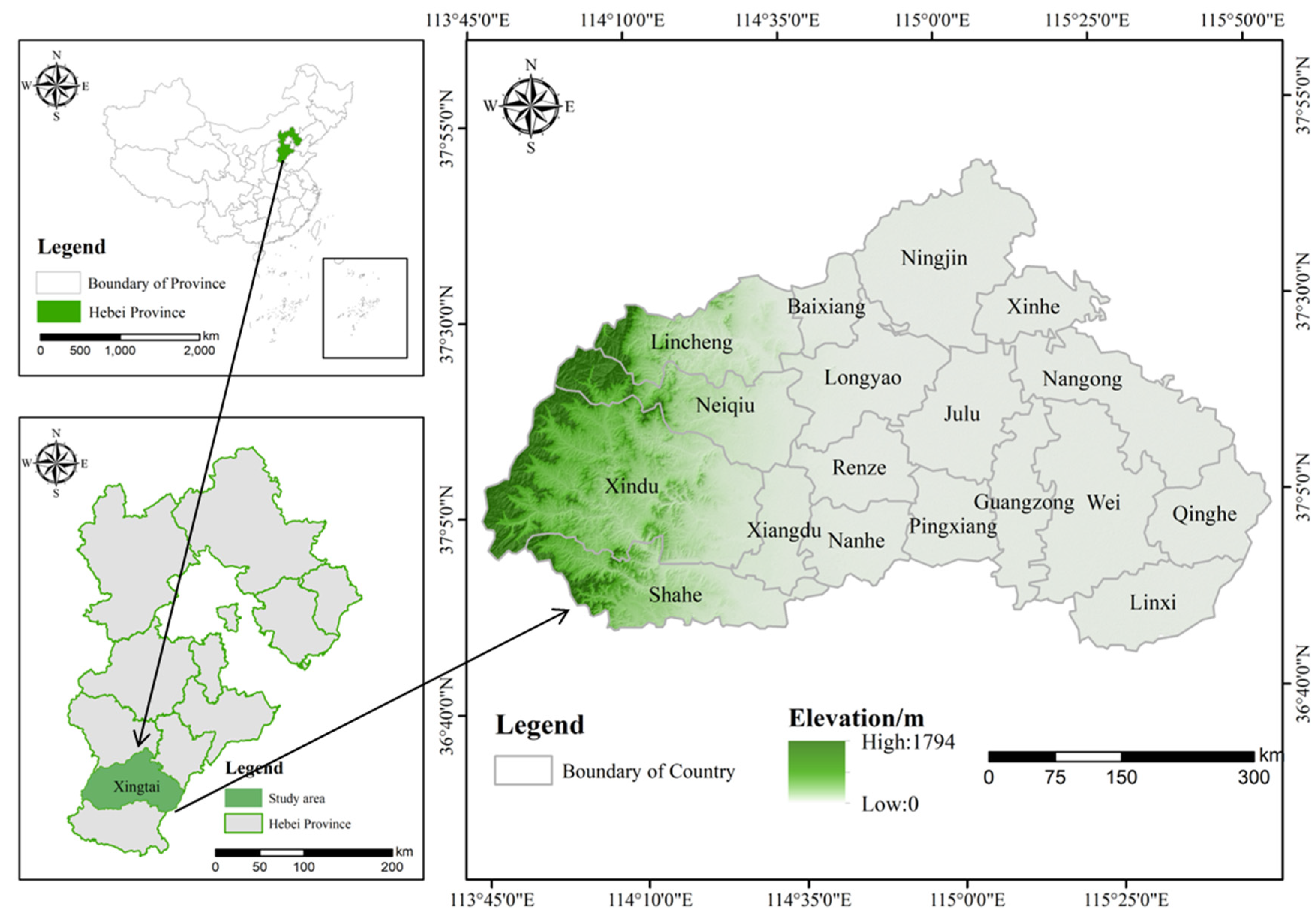
Figure 1. The location of study area.
Land 14 02270 g001
Figure 2. Land use change and Sankey diagram of Xingtai City from 2000 to 2020.
Land 14 02270 g002
Figure 3. Spatiotemporal distribution of ecosystem service supply from 2000 to 2020.
Land 14 02270 g003
Figure 4. Spatiotemporal distribution of ecosystem service demand from 2000 to 2020.
Land 14 02270 g004
Figure 5. Ecosystem service supply-to-demand ratio map of Xingtai City from 2000 to 2020.
Land 14 02270 g005
Figure 6. Integrated ecosystem service supply-to-demand ratio map of Xingtai City from 2000 to 2020.
Land 14 02270 g006
Figure 7. Ecosystem service cluster classification and land use type proportions within each cluster.
Land 14 02270 g007
Figure 8. Analysis of ecosystem service proportions in each cluster, 2000–2020. The length of each colored sector represents the supply–demand ratio of each ecosystem service, indicating the degree of surplus or deficit relative to demand; the percentage labels show the corresponding deviation values.
Land 14 02270 g008
Figure 9. Redundancy analysis of ecosystem service supply–demand relationships and socio-natural driving factors (2000–2020).Abbreviations: GDP: Gross Domestic Product; POP: Population density; NTL: Nighttime Light Proportion; Crop: Cropland proportion; Forest: Forest proportion; DEM: Digital Elevation Model; Pre: Annual precipitation; Tem: Annual mean temperature; Toc: Organic carbon proportion; Tclay: Clay proportion; Tsand: Sand proportion; Tsilt: Silt proportion; Symbols: Blue arrow: Ecosystem services; Red arrow: Driving factors.
Land 14 02270 g009
Figure 10. Spatial distribution of driving factor regression coefficients.
Land 14 02270 g010
Table 1. Description of model frameworks, input parameters, and supply–demand metrics for six ecosystem services (S: supply, D: demand) models.
ESsModel ProcessParameters Description
WYS: S w y = 1 A x P x × P x S w y = water production service supply (mm); A x = actual annual evapotranspiration (mm).
P x = annual precipitation for raster cell x (mm).
D: D w y = W d o m + W a g r + W e c o + W o t h D w y = the demand for water production services; W d o m , W a g r , W e c o , and W o t h represent industrial and domestic water use, agricultural water use, ecological water use, and other water use.
SRS: S D = R K L S U S L E
U S L E = R × K × L S × C × P
R L K S = R × K × L S
SD = soil retention demand; RKLS = Potential Soil Erosion
USLE = Actual Soil Erosion; R = Rainfall Erosivity Factor
K = Soil Erodibility Factor; LS = Topographic Factor (slope length/steepness).
C = Vegetation Management Factor; P = Anthropogenic Measures Factor.
D: U S L E = R × K × L S × C × P
HQS: S H Q = H j 1 D x j z D x j z + k z S H Q = the level of provision of habitat quality services;
Dxj = the level of stress experienced by raster x in land use type j; H j = the habitat suitability of land use type j.
k = a scaling constant; z = a normalization constant.
D: D H Q = k = 1 M S H Q S
D H Q = D H Q S H Q     S H Q < D H Q                     0             S H Q D H Q
D H Q = the Habitat Quality Requirement Standard.
S = the size of the study area (km2).
UCS: H M i = C C i C C i > C C p a r k i o r   G A i < 2   h a C C p a r k i ( Other   situations . )
C C i = 0.6 × shade + 0.2 × albedo + 0.2 × E T I
C C p a r k i = j dradiusfromi g j × C C j × e d i , j d c o o l
HMi = the supply of heat island regulation services on image i.
CCi = the cooling capacity index, shadowing, evapotranspiration, and albedo [33].
CCparki = the distance-weighted average of the CC values for the greenfield.
dcool = the effective greenfield cooling distance.
D: D H M = P density × max P density 1 × 0.7 + P 65 + × max P 65 + 1 × 0.3 × T D H M = the demand for heat island regulation;
P density = the population density of the administrative unit;
P 65 + = the percentage of the population over 65 years of age in the administrative unit;
T = the mean value of the inversion temperature [34].
PM2.5S: P p m 2.5 = F × L A I × T × 0.5 × V x
F = V p m 2.5 × C p m 2.5
V x = C x × H
P p m 2.5 = Annual PM2.5 Deposition; F = PM2.5 Deposition Flux;
LAI = Annual Leaf Area Index; V p m 2.5 = PM2.5 Deposition Velocity;
C p m 2.5 = Annual PM2.5 Concentration; V(x) = Air Purification Volume (grid x).
C(x) = Grid Area, H = PM2.5 Distribution Height.
D: P D p m 2.5 = C p m 2.5 P B p m 2.5 × T × V x P D p m 2.5 = Required PM2.5 Reduction; C p m 2.5 = Annual PM2.5 Concentration.
P B p m 2.5 = PM2.5 “Excellent” Standard (35 μg/m3) [35,36].
NPPS: N P P x , t = A P A R x , t × ε x , t
A P A R x , t = S O L x , t × 0.5 × F P A R x , t
ε x , t = T ε 1 x , t × T ε 2 x , t × W ε x , t × ε m a x
NPP(x,t) = Net Primary Productivity; APAR(x,t) = Absorbed Photosynthetically Active Radiation; ε(x,t) = Actual Light Use Efficiency; SOL(x,t) = Total Solar Radiation, FPAR(x,t) = Fraction of Absorbed PAR, Tε1(x,t); Tε2(x,t) = Temperature Stress Coefficients;
Wε(x,t) = Water Stress Coefficient; εmax = Maximum Light Use Efficiency.
D: C D = D N x D N s u m × C CD = Carbon Sequestration Demand; D N x = Nighttime Light Value (pixel x)
D N s u m = Total Regional Nighttime Light Value; C = Total Carbon Emissions.
Table 2. Indicator Selection Table.
TypeDriving Factors (Unit)Abbreviation
Natural FactorsAnnual Average Precipitation (mm)Pre
TemperatureTem
Elevation (m)DEM
Soil Organic Matter (%)Toc
Clay ContentTclay
Silt ContentTsilt
Sand ContentTsand
Social FactorsGDP per Unit Area (10,000 yuan/km2)GDP
Socioeconomic Activity Data (Nighttime Light)NTL
Population DensityPop
Proportion of Cultivated Land AreaCrop
Proportion of Forest AreaForest
Proportion of Urban AreaUrban
Table 3. Data Sources.
Data TypeData ResolutionData Source
Land Use30 mResource and Environmental Science Data Platform (http://www.resdc.cn, accessed on 12 September 2025)
Elevation30 mEarth Resources Data Cloud Platform—“Global 30 m SRTM Elevation DEM Data” (www.gis5g.com, accessed on 12 September 2025)
Soil Data1 kmHarmonized World Soil Database (HWSD) V1.2
Precipitation and Evapotranspiration1 kmNational Earth System Science Data Center (http://www.geodata.cn, accessed on 12 September 2025)
Temperature1 kmEarth Resources Data Cloud
Land Surface Temperature1 kmResource and Environmental Science Data Platform
Nighttime Light1 kmEarth Observation Group—Payne Institute for Public Policy (https://www.mines.edu, accessed on 12 September 2025)
Population Density1 kmLandScan 1 km Global Population Distribution Raster Data
GDP and Energy ConsumptionNational Bureau of Statistics of China, China Energy Statistical Yearbook
Annual Average Leaf Area Index (LAI)1 kmEarth Resources Data Cloud—“China 1 km Monthly Average LAI Dataset (2000–2022)” (www.gis5g.com, accessed on 12 September 2025)
PM2.51 kmNational Tibetan Plateau Data Center—“China High-resolution and High-quality PM2.5 Dataset (2000–2023)” (http://www.tpdc.ac.cn, accessed on 12 September 2025)
Population Age Structure, Water UseCounty LevelCounty/City Statistical Yearbooks, Water Resources Bulletins
Table 4. Land use transition matrix of Xingtai City from 2000 to 2020 (km2).
Year 2000 →
Year 2020 ↓
Cultivated LandForest LandGrasslandWater AreaConstruction LandUnused LandTotal Outflow
Cultivated Land7955.33440.775484.716171.4105971.70753.89349127.8369
Forest Land22.8645667.123217.58240.849611.74680.0531720.2196
Grassland86.526998.6112991.742487.658273.33830.32131338.1983
Water Area30.34260.70292.044895.161510.35917.0766155.6874
Construction Land125.90640.53910.98462.0502985.93020.0991115.5095
Unused Land0000000
Total Inflow8220.9744807.75181097.0703257.132053.081821.443412457.4517
Net Change−906.862587.5322−241.128101.4426937.572321.4434
Table 5. Regression parameters for OLS model, GWR model, and GTWR model.
ModelAICcR2R2 Adjusted
OLS1906.40.314-
GWR1206.7850.5150.509
GTWR902.4110.6420.636
Disclaimer/Publisher’s Note: The statements, opinions and data contained in all publications are solely those of the individual author(s) and contributor(s) and not of MDPI and/or the editor(s). MDPI and/or the editor(s) disclaim responsibility for any injury to people or property resulting from any ideas, methods, instructions or products referred to in the content.