Article

The Application of CA–MLP–ANN in Assessing Urbanisation in Quaternary Catchment X22J of Mpumalanga, South Africa

by
Mary Nkosi
1,2,* and
Fhumulani I. Mathivha
1
1
Department of Water and Sanitation, University of Limpopo, Polokwane 0727, South Africa
2
Department of Geography and Environmental Sciences, University of Limpopo, Polokwane 0727, South Africa
*
Author to whom correspondence should be addressed.
Land 2025, 14(11), 2099; https://doi.org/10.3390/land14112099
Submission received: 9 September 2025 / Revised: 16 October 2025 / Accepted: 20 October 2025 / Published: 22 October 2025
(This article belongs to the Special Issue Land Use and Land Cover Change Analysis in Dynamic Landscapes)

Abstract

Quaternary catchment X22J boasts ecological biodiversity, making ecotourism one of the thriving industries in the catchment. However, recent population growth and the migration from rural areas to urban areas have increased urbanisation. Therefore, this study aimed to assess and predict the trajectory of urban growth. Through the random forest algorithm in Google Earth Engine, this study analysed urban use in 1990, 2007 and 2024. The classification achieved an overall score of 0.89, 0.96 and 0.91 for 1990, 2007 and 2024, respectively. In addition, the Kappa coefficient varied between 0.85, 0.83 and 0.87 for 1990, 2007 and 2024. The CA–MLP–ANN algorithm was applied for the prediction of 2040 urban changes, leading to the model achieving a score of an overall Kappa coefficient of 0.52 and 74% correctness. Overall, the study predicted an increase of 4.01% in built-up areas from 2024 to 2040, maintaining the increasing trend from 1990. Consequently, a loss of 11% was observed in agricultural lands and a loss of 0.17 in waterbodies by 2040.

1. Introduction

In developing countries, like South Africa, urbanisation has been associated with advancement in socio-economic standing and lifestyle improvement. For example, Mthiyane et al. [1] highlighted job creation, better housing and public services as some of the positive impacts of urbanisation. However, despite these benefits, urbanisation has been linked to soil degradation, damaged wildlife habitats, and a drastic decrease in biodiversity and ecosystem services. For instance, in South Africa, Deacon et al. [2] reported a decrease in wetland biodiversity following urban expansion in the City of Cape Town. The X22J quaternary catchment is a sub-catchment of the Crocodile River catchment (CRC), which is rich in ecological biodiversity; however, recent population growth and urban influx have increased the rate of urbanisation [3,4], which could potentially affect the rich ecological diversity. Furthermore, Frankson [5] reported on increased urban areas, and their impacts on water usage were documented. At a catchment level, studies such as those by Schütte and Schulze [6] and Phelokazi et al. [7] categorised urbanisation as having the most impact on the hydrological responses and water balance, thus affecting its water intake. Muhammad et al. [8] alluded to population growth as the driver of anthropogenic activities such as industrialisation, urbanisation and resettlement that eventually lead to the modification of the Earth’s terrestrial environment. Ritchie et al. [9] reported that globally, more than 4 billion people are estimated to live in urban areas, and Kapucu et al. [10] further projected that approximately 70% of the world’s population will live in urban areas by 2050. While the South African National Space Agency (SANSA) [11] estimated that 60% of the population was already established in urban areas in 2020, this number is projected to increase to 80% by 2050.
Several land-use simulation and prediction models have been developed to provide a more holistic land-use management approach. The most well-known model types include stochastic discrete models, empirical–statistical models and hybrid models. Stochastic discrete models are spatial land-use models used for the quantification of predicted land-use/cover of a particular region and the responsible driving force (e.g., Cellular Automation (CA), Markov Chain (MC)) [12,13,14]. In contrast, empirical–statistical models are mostly applied in the assessment of existing and expected LULC change patterns and areas of cover [15]; such models mostly simplify the modelling of complex and dynamic systems. Examples of empirical–statistical models include the artificial neural network (ANN) and the support vector machine (SVM) [5,12,16,17]. Hybrid models, e.g., CA–SVM, CA–MC and Multilayer Perceptron (MLP)–ANN [18] were developed by integrating several models to form a single model. For LULC assessment studies, CA and ANN models have been widely used for land-use simulations and predictions [8,19]. ANN-based models can simulate a “nonlinear spatially probabilistic land-use transformation” and facilitate the development of complex LULC models. Basse et al. [19] further highlighted that CA models can effectively simulate LULC systems and their functions, especially when applied in conjunction with other models like ANN. In this view, it can be argued that CA-based spatial models can adequately replicate and forecast the dynamic forces and drivers of urban growth [20].
Increase in water demand due to increasing urbanisation has been linked to the overexploitation of more than 60% of rivers [21], and the CRC is no exception. Despite the documented impacts, urbanisation is inevitable and rapid urban growth is a challenge in South Africa, as pointed out by several studies [22,23,24,25]. Urban development should be sustainable and future-oriented. This is because, according to Kafy et al. [26], unplanned LULC changes, can exacerbate the impacts of climate change by reducing the land available for green cover and further decreasing water resources. Therefore, given the increasing demand for natural resources and the need to protect the environment, modelling and predicting land use are some of the efforts applied toward effective natural resource management [27,28]. The diversification of spatial datasets such as satellite images and the increase in their usability have enabled the development of computer-based software for land-use modelling [27,29]. Agyemang et al. [30] highlighted that determining, monitoring and modelling LULC changes provides insights into the status and trends of LULC and urban growth trajectories, thus equipping urban planners and decision-makers. It can therefore be concluded that models have created an opportunity to improve land-use policies [31], thereby ensuring the balance in the usage and conservation of land, and its sustainability in areas under development pressure [18,27].
As a result of intense industrial and urban land uses, the CRC is said to be water-stressed [3]. Likely, the increase in urbanisation will further exert pressure on this catchment area, thus putting it at risk of degradation. While several studies [32] assessed the impacts of land-use changes and land management on the catchment, most studies focus on historical and present changes, with limited studies predicting future urban change. Nkosi [32], applied the maximum likelihood (ML) algorithm to assess spatial processes of land use and urbanisation at the broad CRC scale. While effective for generalised classification and large-scale pattern recognition, the ML algorithm has inherent limitations in capturing the non-linear, spatially heterogeneous and dynamic interactions that drive urban growth at finer spatial resolutions. Moreover, wider catchment-scale analyses often mask local variations in land-use transition dynamics that are critical at the quaternary catchment scale, where detailed planning and resource management decisions are typically implemented. To address this methodological limitation, the current study applied the CA–MLP–ANN approach, which integrates spatial transition rules with advanced non-linear learning capabilities. The model allows for quaternary-scale simulation and prediction of urbanisation patterns, capturing localised spatial dependencies and complex relationships between driving factors that the ML approach cannot adequately represent.

2. Materials and Methods

2.1. Study Area

The X22J QC shown in Figure 1 is one of the 35 quaternary catchments of the Crocodile River catchment and the only one of the 10 that is urbanised [32]. The catchment is located in the Lowveld region of Mpumalanga Province, and drains an approximate area of 240 km2 with a mean annual precipitation (MAP) of 815 mm. The catchment experiences an annual average temperature of 22 °C and potential evapotranspiration (PET) rates of 2000 mm. The quaternary catchment occupies the fertile valley of the Crocodile River; however, it is also home to the City of Mbombela—one of the fastest-growing cities in South Africa, with an annual growth rate of 2.4% [33]. Apart from this, the study area also houses several suburbs, notably Kamagugu, Riverside and Nelsville, and it is also known as a gateway for eco-adventures, thus making it one of the most preferred tourist destinations in South Africa [34]. The total calculated growth rate for the catchment was 8%. The least urbanised parts of the catchment area host recreational activities and agricultural activities, such as citrus and macadamia plantations.

2.2. Input Data Acquisition

This study made use of the Digital Elevation Model (DEM), population density, open street data, built-up areas and satellite images for land-use analysis and prediction. The DEM, open street, built-up areas, and population data were acquired to produce the spatial driver variable maps used as input to the Modules for Land-Use Change and Evaluation (MOLUSCE) v 5.01 plug-in tool in QGIS v 3.22. All the data were processed in QGIS before being remapped in RStudio (v2025.09.1+401). Depending on the mapping purposes, the variable maps differ per study; however, distance to road and DEM are always important to include in the list. The more spatial variable maps are used, the better the prediction accuracy [35].
Table 1 summarises the data used in the study, the sources, and the data length. The study considered a period of 34 years (1990–2024) and a predicted period of 2040. The 1990 classified map presented the initial LULC map, and it also presented the base period. The year 2007 accounts for the transition period, and it is also reported as the year in which South Africa witnessed a significant increase in urbanisation due to the economic shift [22]. The 2024 classified map was used as the final LULC map for the prediction tool, and it also presents the current LULC state. The MOLUSCE tool forecasts land use by adding the difference between the initial and final maps, multiplied by the number of iterations; thus, 2024 was also used for validation of the simulation. Figure 2 presents the workflow for predicting the LULC for the year 2040 in MOLUSCE.

2.3. LULC Classification and Analysis

Satellite images (e.g., Landsat 4-5-TM and Sentinel-1-2) play an important role in LULC monitoring, analysing historical trends and forecasting simulations, consequently being important in policymaking and promoting sustainable land use and planning [29]. Land-use maps, i.e., 1990 and 2007, were classified from the Landsat-4-5-TM images and year 2024 was classified using Sentinel-1-2. Image pre-processing, processing and post-processing were done on Google Earth Engine (GEE). This included tasks such as clipping to a region of interest (ROI), calculation of the median, dates and metadata filtering and band compositing. The classifications were undertaken using the random forest (RF) algorithm. GEE is a widely used, advanced, cloud-based global open-source platform hailed for its rapid and accurate processing. According to Tesfaya et al. [36], the platform can evaluate multiple satellite images quickly and effectively. Many studies have used it because of this aspect and the fact that all required images can be obtained on one platform [36,37].
GEE comes equipped with numerous machine learning classification algorithms, namely, smile cart, support vector machine (SVM) and traditional approaches such as minimum distance and maximum likelihood [38]. RF is a classification method that builds multiple decision trees using random subsets of data and features, and each tree independently predicts the class of a data point; the final classification is determined by majority voting across all trees [39]. Compared to other algorithms, RF has high accuracy, accounts for both classification and prediction challenges, and is also widely used for land-use classification [37,38]. All model training and testing were concluded on GEE, and classification was done under supervision as per the workflow shown in Figure 2. Only images with cloud covers of less than 1 were selected. The training dataset was divided into 80/20, i.e., 80% was used for training, and validation was done using the remaining 20% of the dataset. Land-use classes considered in this study include built-up areas, cultivation, natural vegetation and waterbodies. For this study, the output mode of the RF classifier was set to ‘multiprobability’ to allow it to generate a probability map for each class, reflecting the likelihood of each pixel belonging to that class. This probabilistic output captures the classifier’s confidence, providing a continuous measure rather than just hard labels. Coupling these uncertainty measures with standard validation metrics improves overall map reliability and addresses uncertainties.

2.4. Land-Use Prediction

2.4.1. Spatial Variable Data

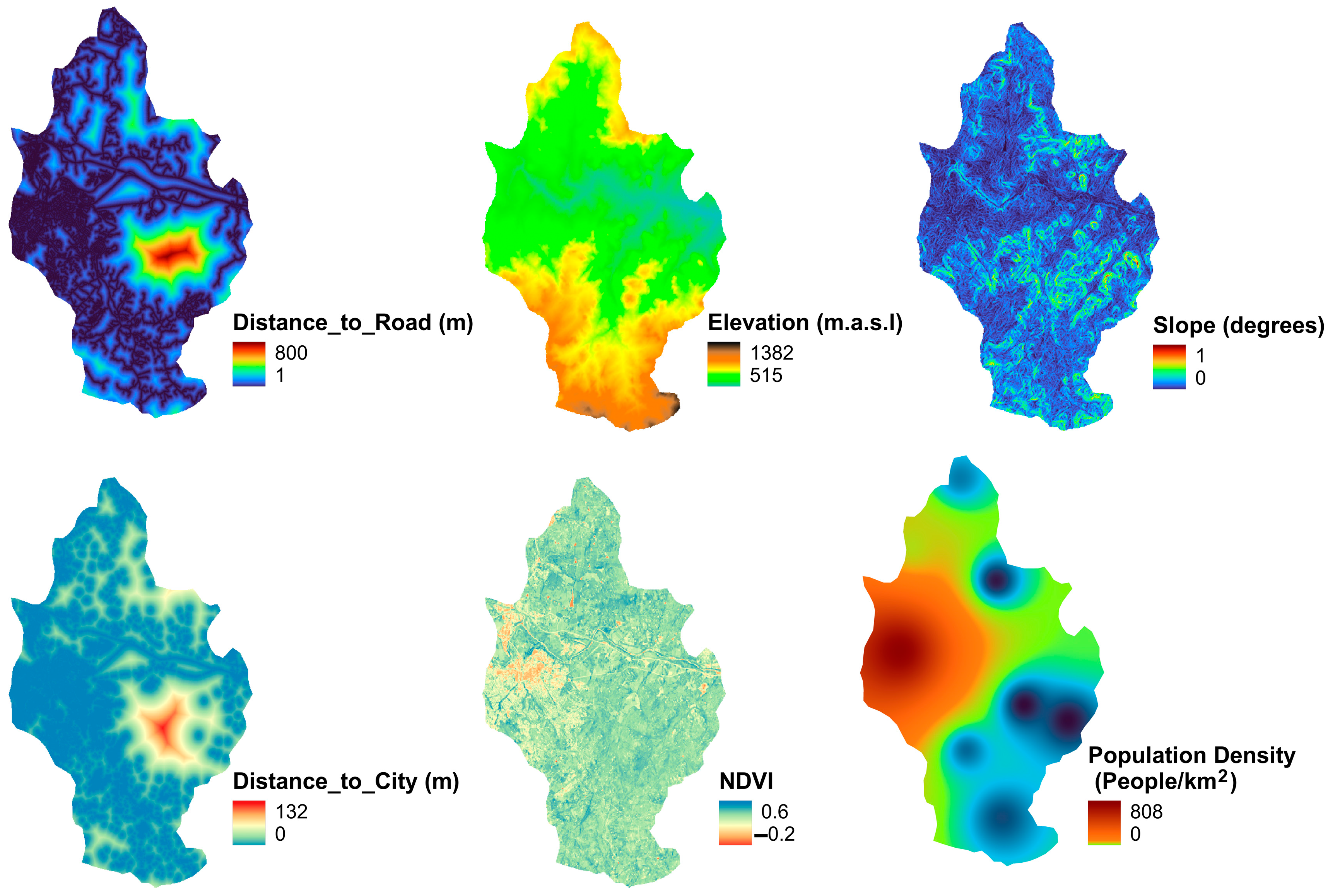
The spatial variables were projected to WGS 84/UTM Zone 36 before resampling in RStudio. Consistency in the resolution of the input data is imperative to allow for processing in the LULC prediction tool; thus, the need for resampling of the spatial data. There are multiple resampling methods, namely, bilinear, bicubic and cubic convolution interpolation, and each is chosen based on the resampling requirement [40]. This study used the nearest-neighbour resampling technique because it does not alter values of the input cells, thus conserving the original data values. Hence, it is the recommended option when dealing with discrete and categorical data like land-use classification, as further pointed out by Ibrahim [40] and Kasahun et al. [41]. The spatial variables were resampled to the elevation and slope resolution, i.e., 30 m. Figure 3 shows the reference resampled spatial data input into the model. The distance to road and population density data were rasterised from vectors, then analysed using the proximity tool in QGIS. Slope, DEM and NDVI were used to account for the environmental factor driving urban changes and distance to road, distance to city, and population density accounted for some socio-economic drivers. Table 2 presents the correlation results of the spatial variable, and a strong relationship was observed between distance to road and distance to city. The observed negative correlations between population density and other covariates (slope, distance to road/city, NDVI, elevation) reflect consistent spatial relationships typical in land-use studies.

2.4.2. The MLP–ANN Algorithm Training

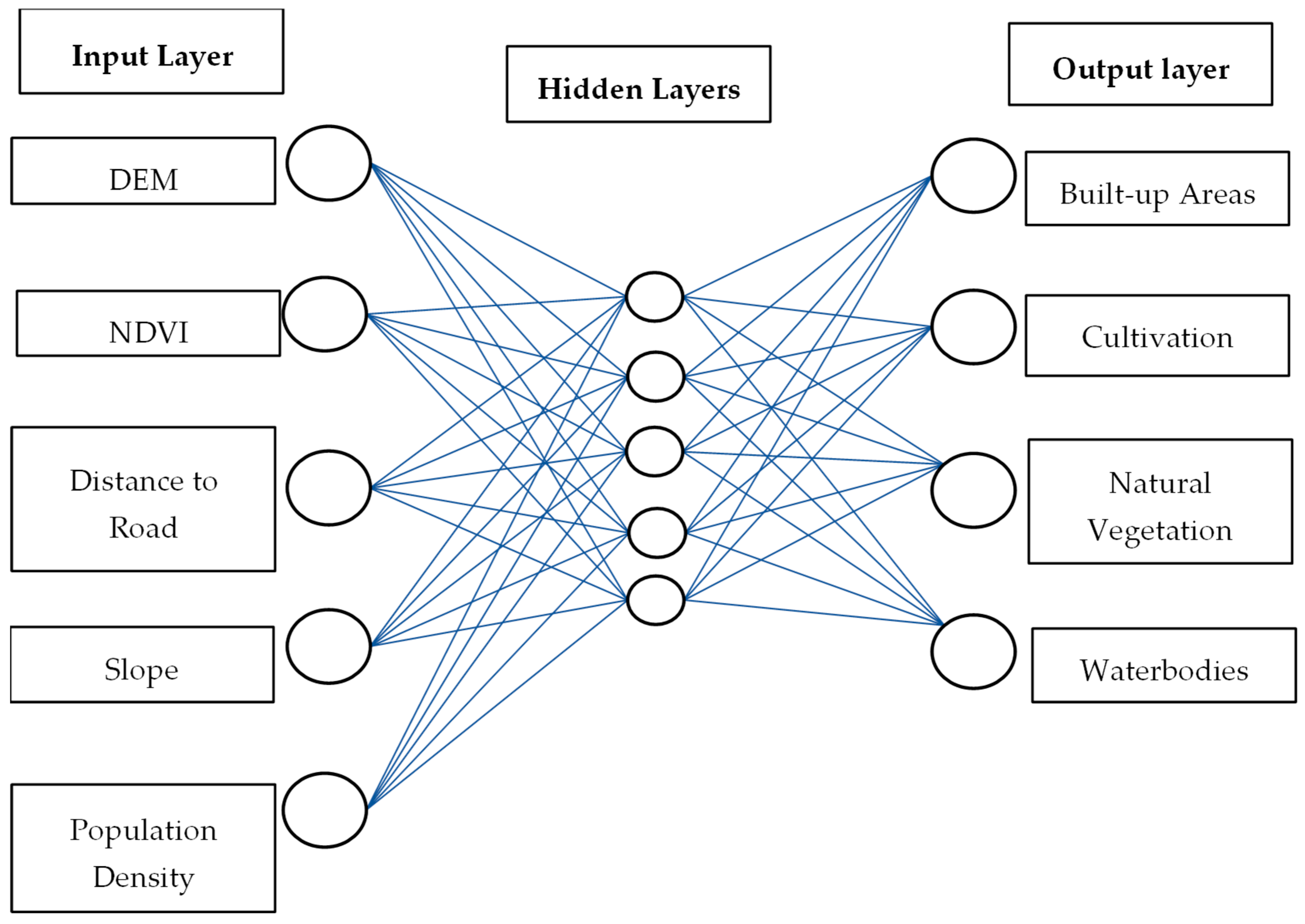
The MLP–CA–ANN in MOLUSCE was trained using the input data, i.e., slope, NDVI, elevation, and distance to the road, and it stopped once the set number of iterations was reached. Training follows the standard back-propagation algorithm, where hidden neurons process weighted inputs from the previous layer to generate activation signals for the next layer [19,42]. These synaptic connections enable the ANN to define transition rules used in CA-based LULC models. Thus, the algorithm has been praised for its ability to model potential transitions based on the input [43]. The tool setup for model training depends on the data complexity of the research, and for this study, the algorithm was trained using 1000 iterations and a neighbourhood value of 0.1 × 0.1 pixels, at a learning rate of 0.01 and 5 hidden layers, and a momentum of 0.05 was selected for modelling the potential transition. Selecting the right learning state, iteration number and hidden layer ensures sufficient model training, reduces overfitting, subsequently ensures accurate model prediction and performance [44]. Thus, The selected model parameters were found to reduce overfitting and reduce uncertainty in data simulation. Figure 4 present the MLP-ANN Architectural structure adopted in this study.
In addition to the MLP–CA–ANN algorithm, MOLUSCE is equipped with multiple algorithms such as multi-criteria evaluation (MCE), logistic regression (LR), and weights of evidence (WoE) [45]. Unlike similar models such as SLEUTH, MOLUSCE is not data-intensive; it is user-friendly and does not have a long calibration process [46]. Globally, it has been applied in the simulation of various scenarios in support of hydrological modelling [8,47]. For instance, Bramantio et al. [48] assessed the dynamics of LULC on the Parangtritis Sand Dunes in Indonesia. The study modelled and predicted changes for the year 2031 with a correctness validation of 92% and a Kappa coefficient of 0.98. These validation performance scores support the success and effectiveness of this tool in predicting LULC—thus its selection in this study and its ability to incorporate the CA–MLP–ANN algorithm.
Figure 4. Architecture of the MLP–ANN model for this study [49].
Land 14 02099 g004

2.4.3. Accuracy Assessment and Prediction Validation

According to Maxwell et al. [50], accuracy assessment is a critical part of land-use classification because it also evaluates the algorithm’s performance in terms of its strengths and weaknesses, and it makes it easy to compare methods. In this study, the accuracy of the classified maps was assessed using the error matrix, user accuracy (UA), producer accuracy (PA) and overall accuracy. The error matrix table, or confusion matrix table, evaluates the accuracy of the classification by comparing the reference classes with the simulated ones. The rows of the table show the true classes, while the columns present the predicted classes [51]. The diagonal row of the table normally presents the pixels that were classified correctly, while the off-diagonal cells indicate the misclassification [52]. Through the confusion matrix table, the UA, PA and OA can be estimated [50]. UA measures the probability of correct results from the user’s perspective and is given by Equation (1), while PA measures the probability of correctly classifying a reference class (see Equation (2)). OA measures the success of the proportion that is correctly classified. The Kappa coefficient accounts for the agreement in classification by comparing the observed accuracy with the expected accuracy due to random chance. Its values range from −1 to 1, where 1 indicates perfect agreement, 0 indicates no better than chance, and negative values indicate worse than chance. The Kappa statistics are calculated using Equation (4).
U s e r   A c c u r a c y = C o r r e c t l y   c l a s s i f i e d   p i x e l s   i n   a   c l a s s   T o t a l   p i x e l s   c l a s s i f i e d   i n   t h a t   c l a s s
P o r d u c e r   A c c u r a c y = C o r r e c t l y   c l a s s i f i e d   p i x e l s   i n   a   c l a s s T o t a l   r e f e r e m c e   p i x e l s   o f   t h a t   c l a s s
O v e r a l l   A c c c u r a c y = T o t a l   c o r r e c t l y   c l a s s i f i e d   p i x e l s T o t a l   r e f r e n c e   p i x e l s
K a p p a   c o e f f i e c i e n t = P a P e 1 P e
where P a presents the proportion of the actual LULC agreement and P e is the expected agreement [43].

2.4.4. Magnitude of Change

The magnitude of change measures the size and direction of land use between two different years. The change detection and magnitude of change were quantified based on the method described by Tola and Deyassa [47], given by Equations (5) and (6).
M a g n i t u d e   o f   C h a n g e = F i n a l   y e a r I n i t i a l   y e a r
%   o f   c h a n g e = M a g n i t u d e   o f   c h a n g e I n i t i a l   y e a r × 100
Negative values presented a decrease, while positive values presented an increase. For this study, Equations (5) and (6) were further used to estimate the level of discrepancies between the forecasted and observed LULC maps.

3. Results

3.1. Accuracy Assessment

3.1.1. Historical Land-Use Classification

As described, the LULC classification was undertaken in GEE and performance matrices were all computed during classification. The overall accuracy for the classified images ranged between 0.89, 0.96 and 0.91 for 1990, 2007 and 2024, respectively. In addition, the Kappa coefficient varied between 0.85, 0.83 and 0.87 for 1990, 2007 and 2024, respectively. When considering the OA, PA, UA and Kappa coefficient, the overall performance of the tool was good; thus, the classifications were found to be within the acceptable threshold as documented by Roy et al. [15] and Tola and Deyassa [47]. Table 3, Table 4 and Table 5 present the confusion matrix for the classified land uses with UA and PA for each land-use class. The overall PA and UA scores ranged between 0.79 and 1. Notably, in terms of built-up areas, the classification of 1990 had a PA of 0.88 while UA was 0.91, indicating that 88% of the classified pixels were within the right class, and the remaining percentage was classified into cultivation land.

3.1.2. Predicted Land-Use Classification Accuracy Assessment

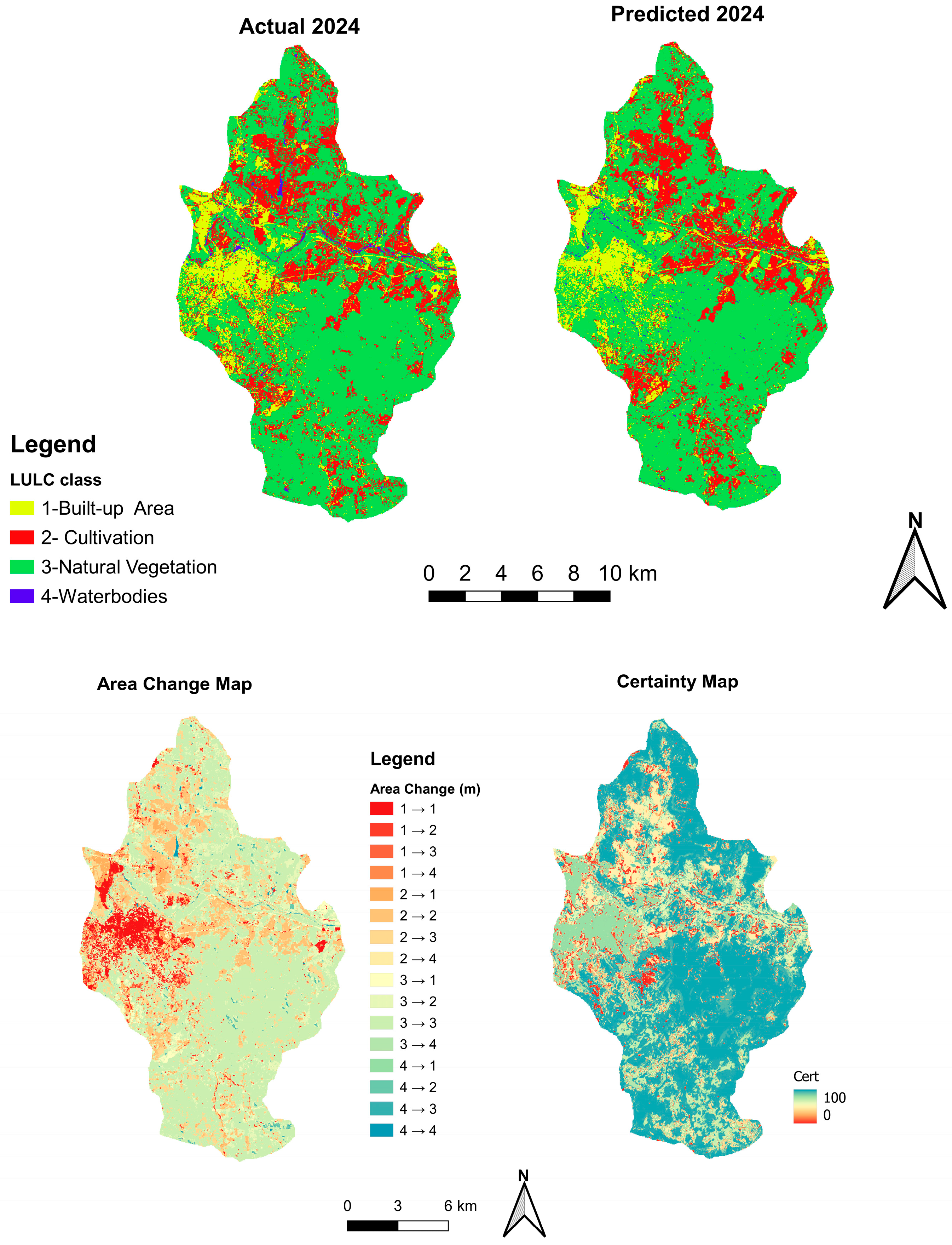
Validation for the predicted LULC maps was carried out by comparing the actual LULC map for the year 2024 with the predicted LULC map for the year 2024. MOLUSCE has inbuilt model validation measures, i.e., the Kappa coefficient and percentage of correctness (overall accuracy), and these are measures produced by the model once processing is done. Figure 5 and Table 6 present the results of the predicted and actual 2024 LULC maps. The prediction scored a Kappa coefficient of 0.52 and an overall score of 0.75. According to Nkolokosa et al. [44], a Kappa score between 0.41 and 0.6 indicates a moderate agreement between the simulated and actual map. The error matrix table shows a UA ranging from 0.34 to 0.84, with the lowest observed in waterbodies, and this coincides with the PA score, with an achieved value of 0.54 (see Table 7). Slight discrepancies were observed in the simulation, with the highest being in the natural vegetation class, with an overestimation of 1.66%. A slight underprediction of 0.44% was observed in built-up areas, most likely due to the difference in the classification tools used in mapping the initial and the actual LULC or a misclassification in the initial LULC map [53,54]. Based on the certainty map in Figure 5, the highest uncertainty was observed when mapping built-up areas such as road networks and cultivation areas.

3.2. Change Detection Between 1990 and 2040

Figure 6 and Table 8 present the classified LULC of 1990, 2007 and 2024 and the forecasted LULC of 2040. Based on the results, the built-up areas expanded by 3% between 1990 and 2024, and are expected to increase by 4.1% from 2024 to 2040, while natural vegetation is expected to increase from 63% in the year 2024 to 71% in the year 2040. Cultivation will decrease from 23% in 2024 to 12% in the year 2040.
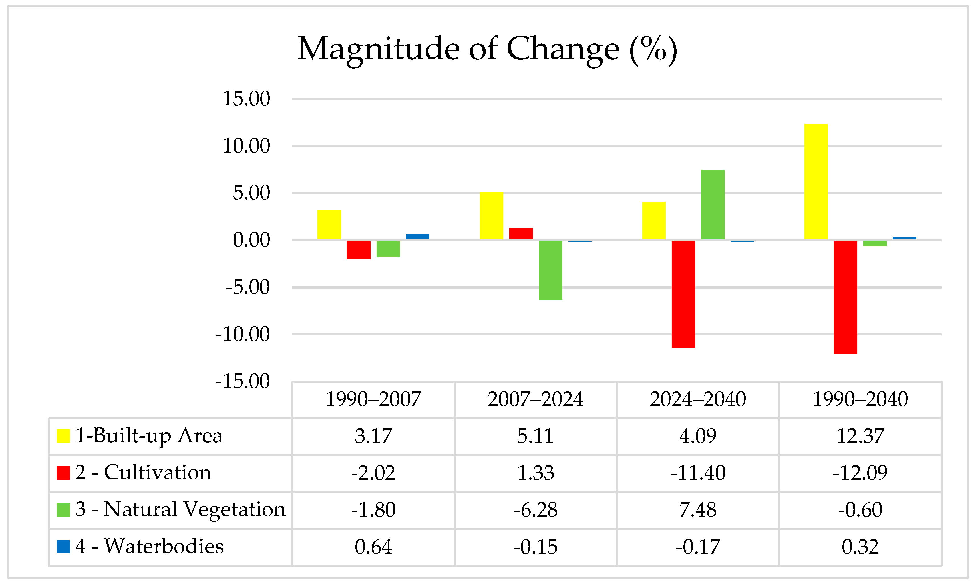
Figure 7 shows the magnitude of change of the four LULC classes considered in this study between the periods 1990–2007, 2007–2024, 2024–2040 and 1990–2040. Based on Figure 7, the magnitude of change for built-up areas has been gradually increasing through the years, and this trend is expected to continue, while natural vegetation depicts the opposite. Table 9 presents the transition probability in LULC between the periods of 1990–2007, 2007–2024, 2024–2040 and 1990–2040. The table quantifies the likelihood that land use will remain stable or transition from one class to the next over a specified period [55]. Overall, the results show that 70% of the built-up area will remain stable for the year 2040 from 2024, while 40% will be transitioned to waterbodies, and 10% of cultivation land will be transitioned to built-up areas and 20% will be transitioned from natural vegetation. The transition between agriculture and urban land use signifies the competition for land between the two classes in the catchment, as documented by the Mpumalanga report [34].

4. Discussion

Agyemang et al. [30] highlighted that determining, monitoring and modelling LULC changes provides insights into the status and trends of LULC, and urban growth trajectories of land use/cover, thus equipping urban planners and decision-makers. This study used the RF algorithm in GEE to analyse LULC changes, with emphasis on urban use (built-up areas) for the period between 1990 and 2024. It further employed the ANN–MLP–CA algorithm in the MOLUSCE plug-in tool in QGIS to predict built-up area changes for the year 2040 in the X22J quaternary catchment.
In most cases, the increase in urbanisation is linked to the loss of other LULC classes as observed in Multan, Pakistan, by Hussain et al. [56]. The results of this study indicate a notable increase in built-up areas, accompanied by a decline in cultivation land between 2024 and 2040 (refer to Figure 6). Specifically, the expansion in built-up areas is predicted to cause an 11.4% reduction in cultivation land by 2040 compared to 2024, suggesting a significant conversion of agricultural land into residential and urban uses. This trend is likely driven by population growth pressures, as evidenced by a projected 4.09% increase in built-up areas by 2040 (see Figure 8).
Similar studies undertaken on the subject matter have observed similar trends in built-up areas with a loss in vegetated area [8,56]. For instance, Hussain et al. [56] predicted an increase of 10% in built-up areas from 2020 to 2050 using the CA–Markov Model in Multan, Pakistan. Değermenci [57] used the MOLUSCE tool to project an increase of 52% in artificial surface by 2054 from 2022 in a study conducted in a 5 km radius circle of the city centre. The latter noted population as one of the major drivers of these changes.
Like the conducted studies [8,56,57], this study noted population growth as one of the drivers of urbanisation. The Mbombela Local Municipality (MLM), where this catchment is located, had an estimated population of approximately 612,927 in 2014, which is expected to increase to around 818,172 by 2035 according to municipal projections. This population increase is fueling urban expansion, thus encroaching on agricultural lands. In response, the city plans to enhance the capacity of its city centres by 2030 to accommodate additional commercial and residential developments, aiming to manage this growth sustainably [City of Mbombela] [33,58]. This further shows the influence of policy frameworks in urban growth. Figure 8 presents the population trend from 1990 to 2050 in relation to the modelled built-up areas.
In addition to population growth, industrialisation is another notable cause of the rapid expansion in impervious surfaces [59]. For instance, the transition from an agricultural zone to an industrial zone demands more urban housing, parking lots and roads. The Maputo Development Corridor (MDC) is an example of such an infrastructure initiative motivated by industrialisation. The corridor has led to rapid commercial expansion in Nelspruit and increased economic activities, stimulating urban growth. This is also shown by the strong influence of distance to road and cities’ spatial variables on the model prediction. Improved accessibility, such as upgraded N4 highway, railway lines, telecommunications and the Kruger Mpumalanga International Airport, contributes significantly to urbanisation by improving accessibility and attracting investment and business activities.

5. Limitations of the Model

Although this study managed to capture and predict most of the land use, deviations in predictions were observed when comparing the actual and simulated 2024 classified land use, thus achieving a Kappa score of 0.52. This deviation could have been due to several reasons, such as misclassification in the initial LULC map. A study reported that prediction errors could also be a result of pixel discrepancies [54]; thus, this highlights the importance of quality input data. To improve output results and strengthen the model accuracy, it is recommended that input data be assessed for any pixel misclassification and that researchers ensure that socio-economic data is up to date. Furthermore, advanced statistical techniques should be applied to assess the quality of the input data. With respect to techniques, studies with similar findings recommended an increase in iteration number and improved spatial resolution [60]. The aim of this study was to assess changes in built-up areas and predict the changes for the year 2040. The quantification of socio-economic drivers was outside the scope of the study; thus, it is recommended that future studies dive deeply into analysing the socio-economic drivers of urban growth.

6. Conclusions

The application of the CA–MLP–ANN algorithm in this study robustly predicted an expansion in built-up areas of 4.1% by 2040 from 2024, with a Kappa coefficient of 0.52 and an overall score of 0.75. The increase is expected to exert considerable pressure on cultivation lands and waterbodies. This anticipated urban growth is largely fueled by the unprecedented rise in population, manifesting through increased residential development and broader urban sprawl. This study, therefore, concludes that urbanisation is influenced by a complex interplay of diverse factors, encompassing both environmental drivers, such as landscape alterations, and socio-economic determinants, including population growth and policy frameworks. This study further concludes that there is an urgent need for comprehensive policies and strategic interventions aimed at fostering sustainable urban development. Such policies must prioritise the protection and restoration of vital ecosystem services to preserve biodiversity and ecotourism potential, while simultaneously safeguarding agricultural lands that are critical for food security and socio-economic well-being. Achieving this balance requires a holistic, multidisciplinary and multisectoral approach, integrating environmental science, urban planning, socio-economic policy and community engagement to ensure that urban expansion proceeds in harmony with ecological sustainability. Only through coordinated efforts across sectors and scales can sustainable urban growth be realised.

Author Contributions

Conceptualisation, M.N. and F.I.M.; methodology, M.N.; software, M.N.; validation, M.N.; formal analysis, M.N.; resources, M.N. and F.I.M.; writing—original draft preparation, M.N.; writing—review and editing, M.N. and F.I.M.; supervision, F.I.M.; funding acquisition, M.N. and F.I.M. All authors have read and agreed to the published version of the manuscript.

Funding

This research was funded by the NRF Postgraduate Scholarship [PMDS240629235465].

Data Availability Statement

Original data available from the author on request.

Acknowledgments

During the preparation of this manuscript/study, the authors used Grammarly for the purposes of grammar correction. The authors have reviewed and edited the output and take full responsibility for the content of this publication. The published work is part of an ongoing PhD study registered at the University of Limpopo.

Conflicts of Interest

The authors declare no conflicts of interest. The funders had no role in the design of the study; in the collection, analyses, or interpretation of data; in the writing of the manuscript; or in the decision to publish the results.

Abbreviations

The following abbreviations are used in this manuscript:
ANNArtificial neural network
CACellular Automation
COCGTACo-operative Governance and Traditional Affairs
CRCCrocodile River catchment
CSIRCouncil for Scientific and Industrial Research
DEMDigital Elevation Model
FAOFood and Agriculture Organization
GEEGoogle Earth Engine
GISGeographical Information Systems
LULCLand use and land cover
MAPMean annual precipitation
MDCMaputo Development Corridor
MLPMultilayer Perceptron
MOLUSCEModules of Land Use Change Evaluation
PETPotential evapotranspiration
QCQuaternary catchment
ROIRegion of interest
SANSASouth African National Space Agency
SVMSupport vector machine

References

  1. Mthiyane, D.B.; Wissink, H.; Chiwawa, N. The impact of rural–urban migration in South Africa: A case of KwaDukuza municipality. J. Local Gov. Res. Innov. 2022, 3, 56. [Google Scholar] [CrossRef]
  2. Deacon, C.; Fox, B.; Morland, L.; Samways, M.; Weaver, S.; Massey, R.; Hill, M. Patterns in macroinvertebrate taxonomic richness and community assembly among urban wetlands in Cape Town, South Africa: Implications for wetland management. Urban Ecosyst. 2021, 24, 1061–1072. [Google Scholar] [CrossRef]
  3. Roux, F.; Selepe, M. Ecostatus of the Crocodile River Catchment, Inkomati River System; Department of Water and Sanitation: Pretoria, South Africa, 2013.
  4. Chakwizira, J. Exploring Nelspruit as a Historical Spatial Jigsaw Corridor-Based Secondary City: A Spatial Governance Geographical Perspective. In Secondary Cities and Local Governance in Southern Africa; Matamanda, A.R., Chakwizira, J., Chatiza, K., Nel, V., Eds.; Springer: Cham, Switzerland, 2024. [Google Scholar]
  5. Frankson, L. Hazelmere Dam Water Level Reaches Critical Levels; IFAT Africa: Johannesburg, South Africa, 2015. [Google Scholar]
  6. Schütte, S.; Schulze, R.E. Projected impacts of urbanisation on hydrological resource flows: A case study within the uMngeni Catchment, South Africa. J. Environ. Manag. 2017, 196, 527–543. [Google Scholar] [CrossRef] [PubMed]
  7. Phelokazi, S.; Amoo, O.T.; Ikudayisi, A.; Nakin, M. Investigating Water Balance Configuration in the Urban Areas of Mthatha, South Africa. Sel. Sci. Pap. J. Civ. Eng. 2024, 19, 20240019. [Google Scholar] [CrossRef]
  8. Muhammad, R.; Zhang, W.; Abbas, Z.; Guo, F.; Gwiazdzinski, L. Spatiotemporal Change Analysis and Prediction of Future Land Use and Land Cover Changes Using QGIS MOLUSCE Plugin and Remote Sensing Big Data: A Case Study of Linyi, China. Land 2022, 11, 419. [Google Scholar] [CrossRef]
  9. Ritchie, H.; Samborska, V.; Roser, M. Urbanization: The World Population Is Moving to Cities. Why Is Urbanization Happening, and What Are the Consequences? Our World in Data: Oxford, UK, 2018. [Google Scholar]
  10. Kapucu, N.; Ge, Y.; Rott, E.; Isgandar, H. Urban resilience: Multidimensional perspectives, challenges and prospects for future research. Urban Gov. 2024, 4, 162–179. [Google Scholar] [CrossRef]
  11. SANSA. The Role of Satellite-Based Remote Sensing Technologies in Support of Urban Spatial Planning; SANSA Policy Brief: Pretoria, South Africa, 2019.
  12. Rani, A.; Gupta, S.K.; Singh, S.K.; Meraj, G.; Kumar, P.; Kanga, S.; Ðurin, B.; Dogančić, D. Predicting Future Land Use Utilizing Economic and Land Surface Parameters with ANN and Markov Chain Models. Earth 2023, 4, 728–751. [Google Scholar] [CrossRef]
  13. Wijesekara, G.N.; Gupta, A.; Valeo, C.; Hasbani, J.G.; Qiao, Y.; Delaney, P.; Marceau, D.J. Assessing the impact of future land-use changes on hydrological processes in the Elbow River watershed in southern Alberta, Canada. J. Hydrol. 2012, 412–413, 220–232. [Google Scholar] [CrossRef]
  14. Han, S.; Mao, H.; Dally, W.J. Deep Compression: Compressing Deep Neural Networks with Pruning, Trained Quantization and Huffman Coding. arXiv 2015, arXiv:1510.00149. [Google Scholar]
  15. Roy, S.; Farzana, K.; Papia, M.; Hasan, M. Monitoring and Prediction of Land Use/Land Cover Change using the Integration of Markov Chain Model and Cellular Automation in the Southern Tertiary Hilly Area of Bangladesh. Int. J. Sci. Basic Appl. Res. IJSBAR 2015, 24, 125–148. [Google Scholar]
  16. Wang, Q.; Guan, Q.; Lin, J.; Luo, H.; Tan, Z.; Ma, Y. Simulating land use/land cover change in an arid region with the coupling models. Ecol. Indic. 2021, 122, 107231. [Google Scholar] [CrossRef]
  17. Mungai, L.M.; Messina, J.P.; Zulu, L.C.; Qi, J.; Snapp, S. Modelling Spatiotemporal Patterns of Land Use/Land Cover Change in Central Malawi Using a Neural Network Model. Remote Sens. 2022, 14, 3477. [Google Scholar] [CrossRef]
  18. Ganasri, B.P.; Raju, A.; Dwarakish, G.S. Different Approaches for Land Use Land Cover Change Detection: A Review. PRJET 2023, 2, 44–48. [Google Scholar]
  19. Basse, R.M.; Omrani, H.; Charif, O.; Gerber, P.; Bódis, K. Land use changes modelling using advanced methods: Cellular automata and artificial neural networks. The spatial and explicit representation of land cover dynamics at the cross-border region scale. Appl. Geogr. 2014, 53, 160–171. [Google Scholar] [CrossRef]
  20. Bihamta, N.; Soffianian, A.; Fakheran, S.; Gholamalifard, M. Using the SLEUTH urban growth model to simulate future urban expansion of the Isfahan metropolitan area, Iran. J. Indian Soc. Remote Sens. 2015, 43, 407–414. [Google Scholar] [CrossRef]
  21. Donnenfeld, Z.; Crookes, C.; Hedden, S. A Delicate Balance: Water Scarcity in South Africa; Southern Africa Report; WRC: Pretorisa, South Africa, 2018. [Google Scholar]
  22. Turok, I.; Borel-Saladin, J. Is urbanisation in South Africa on a sustainable trajectory? Dev. S. Afr. 2014, 31, 675–691. [Google Scholar] [CrossRef]
  23. Heidari, H.; Arabi, M.; Warziniack, T.; Sharvelle, S. Effects of Urban Development Patterns on Municipal Water Shortage. Front. Water 2021, 3, 694817. [Google Scholar] [CrossRef]
  24. Gambe, T.R.; Turok, I.; Visagie, J. The trajectories of urbanisation in Southern Africa: A comparative analysis. Habitat. Int. 2023, 132, 102747. [Google Scholar] [CrossRef]
  25. Mpepho, L. Urbanisation and Migration in South Africa: Global Trends. Economy & Politics. 2024. Available online: https://www.meer.com/en/79655-urbanisation-and-migration-in-south-africa-global-trends (accessed on 20 August 2023).
  26. Kafy, A.A.; Saha, M.; Faisal, A.; Rahaman, Z.A.; Rahman, M.T.; Liu, D.; Fattah, M.A.; Al Rakib, A.; AlDousari, A.E.; Rahaman, S.N.; et al. Predicting the impacts of land use/land cover changes on seasonal urban thermal characteristics using machine learning algorithms. Build. Environ. 2022, 217, 109066. [Google Scholar] [CrossRef]
  27. Akdeniz, H.B.; Sag, N.S.; Inam, S. Analysis of land use/land cover changes and prediction of future changes with Land Changes Modeler: Case of Belek, Turkey. Res. Square 2022, 95, 135. [Google Scholar] [CrossRef] [PubMed]
  28. Entahabu, H.H.; Minale, A.S.; Birhane, E. Modeling and Predicting Land Use/Land Cover Change Using the Land Change Modeler in the Suluh River Basin, Northern Highlands of Ethiopia. Sustainability 2023, 15, 8202. [Google Scholar] [CrossRef]
  29. Khawaldah, H.A. Prediction of Future Land Use/Land Cover in Amman Area Using GIS-Based Markov Model and Remote Sensing. J. Geogr. Inf. Syst. 2016, 8, 412–427. [Google Scholar] [CrossRef]
  30. Agyemang, F.S.; Silva, E.; Poku-Boansi, M. Understanding the urban spatial structure of Sub-Saharan African cities using the case of urban development patterns of a Ghanaian city-region. Habitat Int. 2019, 85, 21–33. [Google Scholar] [CrossRef]
  31. Chaudhuri, G.; Clarke, K.C. The SLEUTH Land Use Change Model: A Review. Int. J. Environ. Res. 2013, 1, 89–104. [Google Scholar]
  32. Nkosi, M. Impacts of Land Management on Water Resources in the Crocodile River Catchment, Mpumalanga. Master’s Dissertation, University of Venda, Thohoyandou, South Africa, May 2022. [Google Scholar]
  33. City of Mbombela. Spatial Development Framework Review-Working Document; City of Mbombela: Mbombela, South Africa, 2018.
  34. CSIR. Mbombela Local Municipality: Climate Risk Profile Report. GIZ. 2023. Available online: https://greenbook.co.za/documents/GIZ_RiskProfile_MbombelaLM_Sep2023.pdf (accessed on 20 August 2023).
  35. Buğday, E.; Erkan-Buğday, S. Modeling and simulating land use/cover change using artificial neural network from remotely sensing data. CERNE 2019, 25, 246–254. [Google Scholar] [CrossRef]
  36. Tesfaye, W.; Elias, E.; Warkineh, B.; Tekalign, M.; Abebe, G. Modeling of land use and land cover changes using Google Earth Engine and machine learning approach: Implications for landscape management. Environ. Syst. Res. 2024, 13, 1–6. [Google Scholar] [CrossRef]
  37. Negash, E.D.; Asfaw, W.; Walsh, C.L.; Mengistie, G.K.; Haile, A.T. Effects of land use land cover change on streamflow of Akaki catchment, Addis Ababa, Ethiopia. Sustain. Water Resour. Manag. 2023, 9, 78. [Google Scholar] [CrossRef]
  38. Faheem, Z.; Kazmi, J.H.; Shaikh, S.; Arshad, S.; Mohammed, S. Random forest-based analysis of land cover/land use LCLU dynamics associated with meteorological droughts in the desert ecosystem of Pakistan. Ecol. Indic. 2024, 159, 111670. [Google Scholar] [CrossRef]
  39. Salman, H.A.; Kalakech, A.; Steiti, A. Random Forest Algorithm Overview. Babylon. J. Mach. Learn. 2024, 159, 69–79. [Google Scholar] [CrossRef] [PubMed]
  40. Ibrahim, S. Improving Land Use/Cover Classification Accuracy from Random Forest Feature Importance Selection Based on Synergistic Use of Sentinel Data and Digital Elevation Model in Agriculturally Dominated Landscape. Agriculture 2022, 13, 98. [Google Scholar] [CrossRef]
  41. Kasahun, M.; Legesse, A. Machine learning for urban land use/cover mapping: Comparison of artificial neural network, random forest and support vector machine, a case study of Dilla town. Heliyon 2024, 10, e39146. [Google Scholar] [CrossRef]
  42. Maithani, S. A Neural Network based Urban Growth Model of an Indian City. J. Indian Soc. Remote Sens. 2010, 37, 363–376. [Google Scholar] [CrossRef]
  43. Kamaraj, M.; Rangarajan, S. Predicting the Future Land Use and Land Cover Changes for Bhavani Basin, Tamil Nadu, India Using QGIS MOLUSCE Plugin. Environ. Sci. Pollut. Res. Int. 2022, 29, 86337–86348. [Google Scholar] [CrossRef] [PubMed]
  44. Nkolokosa, C.; Stothard, R.; Jones, C.M. Monitoring and simulating landscape changes: How do long-term changes in land use and long-term average climate affect regional biophysical conditions in southern Malawi? Environ. Monit. Assess. 2023, 195, 1247. [Google Scholar] [CrossRef]
  45. NEXTGIS. MOLUSCE-Quick and Convenient Analysis of Landcover Changes. 2007. Available online: https://nextgis.com/blog/molusce/ (accessed on 20 August 2023).
  46. Alshari, E.A.; Gawali, B.W. Modeling Land Use Change in Sana’a City of Yemen with MOLUSCE. J. Sens. 2022, 2022, 419031. [Google Scholar] [CrossRef]
  47. Tola, B.; Deyassa, G. A modeling approach for evaluating and predicting the impacts of land use land cover changes on groundwater recharge in Walga Watershed, Upper Omo Basin, Central Ethiopia. J. Hydrol. Reg. Stud. 2024, 51, 101659. [Google Scholar] [CrossRef]
  48. Bramantio, B.; Hizbaron, D.R.; Khakhim, N. Prediction of the future landuse and land cover changes in the Parangtritis sand dune: A spatio-temporal analysis using QGIS MOLUSCE. IOP Conf. Ser. Earth Environ. Sci. 2024, 1313, 012014. [Google Scholar] [CrossRef]
  49. Qamar, R.; Zardari, B.A. Artificial Neural Networks: An overview. Meso. J. Comp. Sci. 2023, 130–139. [Google Scholar]
  50. Maxwell, A.E.; Warner, T.A.; Guillén, L.A. Accuracy Assessment in Convolutional Neural Network-Based Deep Learning Remote Sensing Studies—Part 1: Literature Review. Remote Sens. 2020, 13, 2450. [Google Scholar] [CrossRef]
  51. De Diego, I.M.; Redondo, A.R.; Fernández, R.R. General Performance Score for classification problems. Appl. Intell. 2022, 52, 12049–12063. [Google Scholar] [CrossRef]
  52. Prantl, T.; Barthel, T.; Kaiser, D.; Schwinger, M.; Bauer, A.; Kounev, S. Challenges in the evaluation of Earth observation products: Accuracy assessment case study using convolutional neural networks. Remote Sens. Appl. Soc. Environ. 2024, 37, 101420. [Google Scholar]
  53. Talukdar, S.; Eibek, K.U.; Akhter, S.; Ziaul, S.; Towfiqul Islam, A.R.M.; Mallick, J. Modelling fragmentation probability of land-use and land-cover using the bagging, random forest and random subspace in the Teesta River Basin, Bangladesh. Ecol. Indic. 2021, 126, 107612. [Google Scholar] [CrossRef]
  54. Thammaboribal, P.; Triphathi, N.K. Predicting Land Use and Land Cover Change Pathumthani, Thailand: A Comprehensive Analysis from 2013–2023 Using Landsat Satellite Imagery and CA-ANN Algorithm, with Projections for 2028 and 2038. Int. J. Geoinf. 2024, 20, 13–27. [Google Scholar]
  55. Mawenda, J.; Watanabe, T.; Avtar, R. An Analysis of Urban Land Use/Land Cover Changes in Blantyre City, Southern Malawi (1994–2018). Sustainability 2019, 12, 2377. [Google Scholar] [CrossRef]
  56. Hussain, S.; Mubeen, M.; Nasim, W.; Mumtaz, F.; Abdo, H.G.; Mostafazadeh, R.; Fahad, S. Assessment of future prediction of urban growth and climate change in district Multan, Pakistan using CA-Markov method. Urban Clim. 2023, 53, 101766. [Google Scholar] [CrossRef]
  57. Değermenci, A.S. Spatio-temporal change analysis and prediction of land use and land cover changes using CA-ANN model. Environ. Monit. Assess 2023, 195, 1229. [Google Scholar] [CrossRef] [PubMed]
  58. City of Mbombela. Climate Change Response Strategy and Implementation Plan (Internal Draft); City of Mbombela: Mbombela, South Africa, 2017.
  59. Bhatta, B. Analysis of Urban Growth and Sprawl from Remote Sensing Data; Springer: Berlin/Heidelberg, Germany, 2010. [Google Scholar] [CrossRef]
  60. Idris, R.; Saleh, M.T.M. Remote Sensing and GIS-Based LULC Prediction in Shah Alam: A Strategy for Sustainable Urban Growth and Development. Bioresour. Environ. 2024, 2, 85–96. [Google Scholar] [CrossRef]
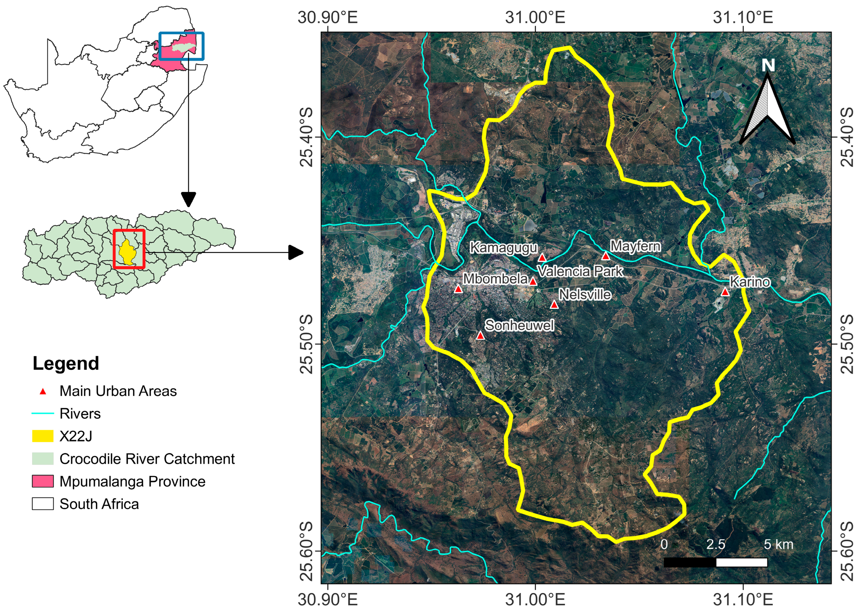
Figure 1. The location of QC X22J and the major towns in the context of South Africa and the Crocodile River catchment.
Land 14 02099 g001
Figure 2. The framework for analysing land-use changes and predicting future LULC.
Land 14 02099 g002
Figure 3. Spatial variable data (i.e., DEM, slope, NDVI, distance to city, population density and distance to the road) input to MOLUSCE.
Land 14 02099 g003
Figure 5. The actual LULC vs. predicted LULC for the year 2024 in QC X22J of Mpumalanga Province. The certainty map and the area change from 1990 to 2024.
Land 14 02099 g005
Figure 6. Classified land-use changes for 1990 and 2023 and the forecasted LULC changes for the year 2040.
Land 14 02099 g006
Figure 7. The magnitude of change between periods.
Land 14 02099 g007
Figure 8. The population and built-up trend from 1990 and 2050.
Land 14 02099 g008
Table 1. Description of data required for the study, acquisition sources and resolutions.
Data TypeDescriptionSourceResampled Resolution
DEMAdvanced Land Observing Satellite (ALOS) World 3D-30m Digital Surface Model (DSM)Japan Aerospace Exploration Agency (JAXA)
https://www.eorc.jaxa.jp/ALOS/en/dataset/aw3d30/aw3d30_e.htm
(accessed on 15 April 2023)
30
Satellite ImagesLandsat 4-5 TM (for 1990, 2007)
Sentinel-1-2 (or 2024)
Google Earth Engine (GEE)
https://code.earthengine.google.com/
(accessed on 04 May 2024)
30
Population DataThe latest population and population density data were used to create the population density variable mapStatistics of South Africa (Stats SA)
https://www.statssa.gov.za/?page_id=993&id=mbombela-municipality
(accessed on 16 May 2024)
30
Open Street DataThe latest open street data were used as a spatial variable for land-use predictionHumanitarian Data Exchange
https://data.humdata.org/dataset/hotosm_zaf_roads
(accessed on 20 August 2023)
30
Built-up AreasExtracted from the South African National Land Cover dataDepartment of Forestry, Fisheries, and Environment
https://www.dffe.gov.za/egis
(accessed on 20 August 2023)
30
Table 2. Evaluating the correlation between spatial variables.
SlopeDistance to RoadDistance to CityNDVIDEMPop Density
Slope 0.270.220.190.28−0.22
Distance to Road 0.840.2−0.04−0.29
Distance to City 0.12−0.05−0.27
NDVI 0.1−0.4
DEM −0.28
Population Density
Table 3. Confusion matrix for 1990 land-use classification.
Class1-Built-Up2-Cultivation3-Natural Vegetation4-WaterTotal
1-Built-Up2121024
2-Cultivation2251028
3-Natural Vegetation0239041
4-Water0041519
Total23294515112
Producer0.880.890.950.79
User0.910.860.861
Bold the names of subheadings of the table and LULC classes.
Table 4. Confusion matrix for 2007 land-use classification.
Class1-Built-Up2-Cultivation3-Natural Vegetation4-WaterTotal
1-Built-Up2911031
2-Cultivation1312034
3-Natural Vegetation0037037
4-Water0002020
Total30324020122
Producer0.940.9111.00
User0.970.970.931.00
Bold the names of subheadings of the table and LULC classes.
Table 5. Confusion matrix for 2024 land-use classification.
Class1-Built-Up2-Cultivation3-Natural Vegetation4-WaterTotal
1-Built-Up4841053
2-Cultivation1495055
3-Natural Vegetation5269379
4-Water0101920
Total54567522207
Producer0.910.890.900.95
User0.870.890.921.00
Bold the names of subheadings of the table and LULC classes.
Table 6. Percentage of cover for the predicted and actual 2024 LULC and the magnitude of discrepancy.
Land-Use ClassSimulated 2024 (%)Predicted 2024 (%)The Magnitude of Change (Discrepancy)
1-Built-Up Area12.5212.080.44
2-Cultivation23.3122.261.05
3-Natural Vegetation63.3264.98−1.66
4-Waterbodies0.850.680.17
Table 7. Confusion matrix for the predicted 2024 LULC.
Class1-Built-Up2-Cultivation3-Natural Vegetation4-WaterTotal
1-Built-Up22,4863572498687531,919
2-Cultivation397634,32220,26137958,938
3-Natural Vegetation641124,486140,809338172,044
4-Water841807258071796
Total32,95762,560166,7812399264,697
Producer0.700.580.820.45
User0.680.550.840.34
Table 8. Changes in LULC from 1990 to 2040.
Class1990 (%)2007 (%)2024 (%)2040 (%)
1-Built-Up471317
2-Cultivation24222312
3-Natural Vegetation71706371
4-Water0111
Total100100100100
Table 9. Probability of change between periods.
2007 2024
1990Class1-Built-Up2-Cultivation3-Natural Vegetation4-Water2007Class1-Built-Up2-Cultivation3-Natural Vegetation4-Water
1-Built-Up0.60.20.201-Built-Up0.70.10.20
2-Cultivation0.10.50.402-Cultivation0.10.50.40
3-Natural Vegetation00.10.803-Natural Vegetation0.10.20.80
4-Water0000.84-Water0.10.30.30.3
2040 2040
2024Class1-Built-up2-Cultivation3-Natural Vegetation4-Water1990Class1-Built-up2-Cultivation3-Natural Vegetation4-Water
1-Built-Up0.70.10.201-Built-Up0.60.10.20
2-Cultivation0.10.50.402-Cultivation0.20.40.40
3-Natural Vegetation0.10.20.803-Natural Vegetation0.10.20.70
4-Water0.40.20.10.34-Water0.200.60.1
Disclaimer/Publisher’s Note: The statements, opinions and data contained in all publications are solely those of the individual author(s) and contributor(s) and not of MDPI and/or the editor(s). MDPI and/or the editor(s) disclaim responsibility for any injury to people or property resulting from any ideas, methods, instructions or products referred to in the content.