Upscaling of Soil Moisture over Highly Heterogeneous Surfaces and Validation of SMAP Product

Abstract

Soil moisture (SM) is a critical component of the global water cycle, profoundly influencing carbon fluxes and energy exchanges between the land surface and the atmosphere. NASA’s Soil Moisture Active/Passive (SMAP) mission provides soil moisture products at the global scale; however, validation of SMAP faces significant challenges due to scale mismatches between in situ measurements and satellite pixels, particularly in highly heterogeneous regions such as the Qinghai–Tibet Plateau. This study leverages high-spatiotemporal-resolution Harmonized Landsat–Sentinel-2 (HLS v2.0) data and the QLB-NET observation network, employing multiple machine learning models to generate pixel-scale ground-truth soil moisture from in situ measurements. The results indicate that XGBoost performs best (R = 0.941, RMSE = 0.047 m³/m³), and SHAP analysis identifies elevation and DOY as the primary drivers of the spatial patterns and dynamics of soil moisture. The XGBoost-upscaled soil moisture was employed as a validation benchmark to assess the accuracy of the SMAP 9 km and 36 km products, with the following key findings: (1) the proposed upscaling method effectively bridges the scale gap, yielding a correlation of 0.858 between the 36 km SMAP product and the pixel-scale soil moisture reference derived from XGBoost, surpassing the 0.818 correlation obtained using the traditional in situ averaging approach; (2) descending-orbit data generally outperform ascending-orbit data. In the 9 km SMAP product, 15 descending-orbit grids meet the scientific standard, compared to 10 ascending-orbit grids. For the 36 km product, only descending orbits satisfy the scientific standard.

1. Introduction

The Qinghai–Tibet Plateau, owing to its unique geographical location and complex topographic features, plays a critical role in global climate change. As a key component of the terrestrial system, soil not only supports plant growth but also connects the atmosphere, biosphere, hydrosphere, and lithosphere, making it an essential part of the Earth’s critical zone. Among its various physical properties, soil moisture (SM) is particularly important as a temporally variable water storage influenced by fundamental hydrological processes, such as precipitation and evaporation, and it regulates infiltration and runoff generated by rainfall [1]. Additionally, it affects the proportion of net radiation allocated to latent heat through its influence on evaporation, thereby impacting atmospheric conditions [2]. In hydrological models, soil moisture serves as an input parameter reflecting the initial water conditions of a watershed and is a critical component of the water balance equation, reflecting the antecedent conditions of a watershed and significantly influencing infiltration and runoff. Wood [3] noted that estimates of grid-scale evapotranspiration are highly sensitive to variations in soil moisture at the sub-grid scale. At medium scales, such as watersheds, variations in surface soil moisture influence the infiltration and runoff generation processes of precipitation, thereby exerting a strong control on runoff forecasting. In agricultural production, soil moisture is a critical indicator for assessing agricultural drought, and its spatiotemporal distribution and variability play an essential role in drought forecasting, crop planning, and agricultural decision-making. Furthermore, soil moisture is indispensable in the contexts of climate change [2] and ecosystem functionality [4].

Traditional soil moisture observations, primarily based on in situ point measurements, can capture soil moisture variations at small scales. However, at larger scales, soil moisture exhibits significant spatial heterogeneity, and single-point observations cannot represent the soil moisture distribution over large areas or cover diverse underlying surface types. The development of remote sensing technology has enabled large-scale soil moisture monitoring, leading to the creation of numerous global-scale soil moisture products. Current soil moisture products are primarily derived from passive microwave data inversion, such as the AMSR-E 25 km soil moisture remote sensing products independently retrieved by NASA, the Vrije Universiteit Amsterdam (VUA), and the Japan Aerospace Exploration Agency (JAXA) using different algorithms and microwave channels [5,6,7]. The Soil Moisture and Ocean Salinity (SMOS) mission is an initiative led by the European Space Agency (ESA) that has provided global soil moisture remote sensing products since 2009, with a temporal resolution of 3 days and a spatial resolution of 40 km [8]. Launched in February 2015 by employing an L-band microwave radiometer and a synthetic aperture radar, the Soil Moisture Active Passive (SMAP) mission is capable of delivering global soil moisture data with a spatial resolution of 36 km. However, the Qinghai–Tibet Plateau is characterized by dramatic topographic variations and high spatiotemporal heterogeneity in soil moisture distribution. Existing soil moisture products show limitations in representing ground-scale soil moisture truth values, especially over highly heterogeneous underlying surfaces. Therefore, the accuracy and applicability of these products in regions with high heterogeneity have become an emerging research focus. However, a fundamental challenge lies in the spatial scale mismatch between satellite-derived soil moisture products and in situ measurements. Direct comparisons between pixel-based satellite data and point-scale ground observations are inherently inappropriate. Bridging the gap between ground-based point measurements and satellite pixel-scale data to provide reliable ground truth at the pixel level represents a key challenge addressed in this study.

The commonly used methods are as follows: (1) Direct validation based on multi-point observations: Currently, most validation studies employ a simple averaging method, which involves directly comparing the time series of shallow soil moisture observations from in situ sites with remotely sensed soil moisture products for accuracy assessment [9]. The simple averaging method is straightforward and computationally convenient. However, in the presence of high spatial heterogeneity of soil moisture over non-uniform underlying surfaces, the accuracy and reliability of this method rapidly decline. (2) Direct validation based on temporal stability analysis: This method assumes that the spatial distribution pattern of soil moisture within the study area remains constant. One or more site combinations are identified as “representative sites” to derive an area-averaged value, which serves as the ground truth for the microwave pixel scale [10,11]. These representative sites are used to represent the regional mean. (3) Validation based on scale extension: With the development of wireless sensor network technology, an adequate number of ground observations can represent the spatial correlation characteristics of soil moisture, using methods such as regression kriging [12] and kriging with unequal observation errors [13]. By integrating remote sensing auxiliary data, improved upscaling results can generally be achieved. Qin et al. [14] combined MODIS thermal inertia with a Bayesian regression estimation method for upscaling, finding that the Bayesian regression approach outperformed the ordinary least squares method, effectively mitigating overfitting and suppressing random errors. Chen et al. [15] utilized Landsat data and applied a Random Forest model to obtain the final upscaled results. Despite the widespread use of MODIS and Landsat data in soil moisture inversion, both datasets exhibit significant limitations in spatial and temporal resolution. MODIS data are characterized by a relatively low spatial resolution, with soil moisture products typically generated at a 1 km scale [16,17], which fails to adequately represent soil moisture spatial heterogeneity. Although Landsat provides a higher spatial resolution of 30 m, its low temporal resolution and limited data availability hinder its use, particularly in high-altitude regions such as the Tibetan Plateau, where the average annual cloud cover can reach approximately 87% [18], further restricting its usability [19]. In order to overcome the spatiotemporal limitations of single-sensor data, this study introduces the Harmonized Landsat–Sentinel-2 (HLS v2.0) surface reflectance product provided by NASA [20]. The HLS v2.0 dataset integrates data from four satellites—Landsat-8/9 and Sentinel-2A/B—achieving a spatial resolution of 30 m and a global median revisit frequency of approximately 2.9 days (excluding Antarctica). This fusion not only retains spatial detail but also significantly enhances temporal continuity. Therefore, HLS v2.0 is considered an ideal data source that combines high spatial accuracy with high temporal sampling capabilities, providing a solid data foundation for conducting fine-scale soil moisture upscaling research in regions characterized by high cloud cover and complex terrain, such as the Qinghai–Tibet Plateau.

In recent years, machine learning (ML) has shown great promise for mapping complex and nonlinear relationships between surface reflectance, terrain, meteorological variables, and soil moisture [19,21,22]. Compared with traditional physically based models, ML techniques require fewer assumptions and can integrate heterogeneous data sources to achieve high-accuracy predictions. Ensemble learning methods (e.g., Random Forest, Gradient Boosting) and neural networks have been widely adopted in soil moisture estimation, outperforming conventional regression techniques. However, most ML-based studies either focus on relatively homogeneous areas (e.g., farmlands or grasslands) or fail to validate results against independent satellite products, limiting their applicability in complex terrains.

This study employs Harmonized Landsat–Sentinel-2 (HLS v2.0) data and multiple machine learning models to develop soil moisture-related indices, construct a fine-scale (30 m) soil moisture upscaling model, and validate regional SMAP soil moisture products. Specifically, the study will (1) construct soil moisture-related indices using HLS v2.0 reflectance data; (2) estimate 30 m surface soil moisture by training multiple machine learning models with in situ measurements and auxiliary variables; (3) identify the optimal model for fine-scale soil moisture retrieval; and (4) validate SMAP products using high-resolution soil moisture estimates derived from the optimal model, thereby assessing their applicability in highly heterogeneous regions. Through this approach, the study aims to provide a scalable and accurate reference for evaluating satellite-based soil moisture products under complex surface conditions.

The main contribution of this study lies in integrating the high spatiotemporal resolution of HLS v2.0 data with advanced machine learning approaches to generate fine-scale soil moisture estimates, which serve as a reliable benchmark for evaluating SMAP products. The inclusion of orbit-level validation further enhances the robustness and practical relevance of the assessment, providing a new pathway for evaluating and improving satellite-based soil moisture retrievals in highly heterogeneous regions.

2. Materials and Methods

2.1. Study Area

The study area is situated within Tianjun County, Haixi Mongolian and Tibetan Autonomous Prefecture, Qinghai Province, China. Located in the northeastern Qinghai–Tibet Plateau, it is bounded by Qinghai Lake (China’s largest inland lake) to the southeast, the Qaidam Basin (one of China’s four major basins) to the west, and the Qilian Mountains (forming part of the northeastern plateau margin) to the northeast. This rectangular region spans 40 km × 36 km (98.96°E–99.34°E, 37.23°N–37.61°N), covering an area of 1440 km². Elevation ranges from 3300 m to 4342 m, with a mean elevation of 3650 m. The terrain is characterized by higher elevations in the north and lower elevations in the south (Figure 1). Specifically, the southern sector comprises hilly grasslands; the southwest contains Tianjun County town and the Buha River; and a wetland is present in the southeast. Topographic complexity increases toward the central area, featuring more mountainous terrain. The northern part is dominated by mountains and valleys, while the northeastern plateau summit hosts extensive alpine meadow wetlands, constituting a highly heterogeneous underlying surface.

2.2. Research Data

The datasets utilized in this study include in situ soil moisture, SMAP soil moisture products, HLS v2.0 surface reflectance data, and digital elevation model (DEM) data. The temporal coverage of all datasets spans 1 September 2019, to 31 December 2023.

2.2.1. In Situ Data

QLB-NET was deployed in September 2019 [23]. This high-density network comprises 60 observational nodes, each equipped with Campbell Scientific CS655 sensors. These sensors simultaneously measure soil temperature, volumetric water content (VWC), and bulk electrical conductivity (EC). Sensors were installed at depths of 5 cm, 10 cm, and 30 cm, recording data at a 30-min temporal resolution. The spatial distribution of the nodes was determined using an optimized sampling scheme specifically designed to meet the validation requirements of major satellite-based soil moisture products, including SMAP, SMOS, AMSR2, ESA CCI, and FY-3B/FY-3C. To support the validation of high-resolution soil moisture products, two intensive 1 km × 1 km observation areas were added in 2020. Within each intensive area, 11 observational sites were established based on a systematic sampling design. This study utilizes data exclusively from the 60 nodes of the primary network. Specifically, only the 5 cm depth soil moisture (VWC) measurements recorded during the unfrozen period (as defined later) are used for processing and analysis.

The Campbell Scientific CS655 sensors measure soil moisture using the time domain reflectometry (TDR) technique. To improve measurement precision, a total of 109 intact soil samples were collected at a 10 cm depth from various locations during September 2019 and July 2020 for calibration experiments. The actual soil moisture content, determined by the ring-knife method, was employed to establish a conversion relationship with the sensor readings. Based on the resulting calibration, soil moisture data from CS655 sensors installed at three depths across 60 large-network and 22 small-network stations were adjusted using a regression coefficient of 1.072. Detailed procedures for calibration and validation can be found in the work of Chai et al. [23].

2.2.2. HLS Data

Harmonized Landsat–Sentinel (HLS) data serve as the cornerstone dataset for constructing the upscaling model in this study, providing high-spatiotemporal-resolution surface reflectance. The reflectance differences in the red, near-infrared, and shortwave infrared bands between the two satellites’ fused data are less than 4%, and the differences in vegetation indices, such as the Normalized Difference Vegetation Index (NDVI) and Enhanced Vegetation Index (EVI), between the sensors are less than 4.5%. Among these, the shortwave infrared bands (including swir1: 1.566–1.651 μm and swir2: 2.107–2.294 μm) are particularly important for soil moisture-related indices, such as the Soil Water Content Index (SWCI), due to the strong absorption of water in these wavelengths. The HLS product consists of two complementary components, HLSL30 and HLSS30, which are spatially and temporally synergistic. Daily data from both components during the unfrozen periods (2019–2023) were spatiotemporally matched and averaged to create a unified composite. All HLS data processing and downloading were performed on the Google Earth Engine (GEE).

2.2.3. DEM Data

The elevation data used in this study were sourced from the NASADEM dataset, a digital elevation model (DEM) reprocessed and refined from the Shuttle Radar Topography Mission (SRTM), with a spatial resolution of 30 m [24]. Based on this dataset, topographic parameters, including slope and aspect, were derived, with all processing and downloading conducted on the Google Earth Engine (GEE).

2.2.4. SMAP SM Product

This research relies on NASA SMAP Level-3 (L3) soil moisture products, including SPL3SMP_E and SPL3SMAP, as the main sources of satellite-based soil moisture data. SMAP captures soil moisture every 2–3 days, capturing soil moisture dynamics over various time scales ranging from major storms to seasonal changes. These products provide global estimates of volumetric soil water content (m³/m³) in the top 0–5 cm soil layer, with SPL3SMP_E offering a spatial resolution of 9 km and SPL3SMAP a spatial resolution of 36 km [25].

SMAP data include both ascending and descending orbit observations, with a substantial difference in the number of records between the two orbits. To maintain consistency with the temporal scale of in situ observations and to comprehensively assess the accuracy of SMAP products, gaps in the SMAP data were filled by averaging the measurements from the preceding and following days. Strict quality control procedures were applied to ensure the accuracy and reliability of the resulting daily soil moisture estimates, which were subsequently used for modeling, validation, and comparison with in situ measurements.

2.3. Methods

To achieve accurate upscaling of soil moisture, this study incorporates multiple independent variables to construct machine learning models (Section 2.3.1) and evaluates the impact of surface heterogeneity in different regions on upscaling performance (Section 2.3.2). Detailed descriptions of the models and the evaluation metrics for the upscaling results are provided in Section 2.3.3 and Section 2.3.4, respectively.

2.3.1. Data Processing

In this study, in situ soil moisture was used as the target variable, while explanatory variables were constructed based on DEM and HLS v2.0 data. The DEM data included elevation, slope, and aspect, while the HLS data—i.e., the reflectance in red (B4), green (B3), blue (B2), near-infrared (B5), and shortwave infrared bands (B6 and B7)—were used to derive indices such as NDVI and SWCI. Given the clear seasonal cycle of soil moisture in the study area, the day of year (DOY, Julian day) was also included as an explanatory variable in the model. To account for the cyclic nature of DOY, sine encoding was applied [26,27]. The formulas for each index are as follows:

$$\begin{array}{c}NDVI={\displaystyle \frac{nir-red}{nir+red}}\end{array}$$

(1)

$$\begin{array}{c}SWCI={\displaystyle \frac{swir1-swir2}{swir1+swir2}}\end{array}$$

(2)

$$\begin{array}{c}\sin DOY= \sin \left(2\mathsf{\pi }\cdot {\displaystyle \frac{DOY}{365}}\right)\end{array}$$

(3)

$$\begin{array}{c}Slope=\arctan \left(\sqrt{{\left({\displaystyle \frac{\partial z}{\partial x}}\right)}^2+{\left({\displaystyle \frac{\partial z}{\partial y}}\right)}^2}\right)\end{array}$$

(4)

$$\begin{array}{c}Aspect={\tan }^{-1}\left({\displaystyle \frac{\partial z/\partial x}{\partial z/\partial y}}\right)\end{array}$$

(5)

where ${\displaystyle \frac{\partial z}{\partial x}}$ and ${\displaystyle \frac{\partial z}{\partial y}}$ represent the gradients of elevation in the east–west and north–south directions, respectively. The terms red, nir, swir1, and swir2 refer to the reflectance in the red (0.636–0.673 μm), near-infrared (nir, 0.851–0.879 μm), shortwave infrared 1 (swir1, 1.566–1.651 μm), and shortwave infrared 2 (swir2, 2.107–2.294 μm) bands, respectively.

Considering the differences in magnitude among various data sources, directly inputting raw variables into the model may cause it to assign disproportionately high weights to variables with larger numeric ranges. This could negatively impact the accuracy and stability of the model. Therefore, all explanatory variables in this study were standardized using the Z-score method with the following formula:

$$\begin{array}{c}z={\displaystyle \frac{x-\mathsf{\mu }}{\mathsf{\sigma }}}\end{array}$$

(6)

where $\mu$ and $\sigma$ represent the mean and the standard deviation of the variable, respectively.

This standardization mitigates the impact of variable scales on model performance, facilitates faster convergence during training to improve optimization efficiency, and enhances the robustness and generalization ability of the model [28]. Following preprocessing, the complete dataset was randomly divided, with 70% allocated for training and 30% reserved for testing. No separate validation set was used, as ten-fold cross-validation was applied within the training set to optimize model parameters.

2.3.2. Assessment of Spatial Heterogeneity

The study area exhibits pronounced spatial heterogeneity. Quantitatively assessing this spatial heterogeneity and examining its impact on SMAP data constitute the core focus of this research. The coefficient of variation (CV), commonly used in statistics to measure the relative dispersion of data, can be applied in the spatial domain to effectively capture the fluctuation characteristics of spatial heterogeneity [29]. The specific calculation formula is shown below.

$$\begin{array}{c}CV=\left({\displaystyle \frac{\mathsf{\sigma }}{\mathsf{\mu }}}\right)\times 100\%\end{array}$$

(7)

$\sigma$ and $\mu$ represent the standard deviation and mean of the elevation, respectively.

2.3.3. Machine Learning Models

Random Forest is an ensemble learning method that constructs multiple decision trees and averages their predictions (taking the majority vote for classification) to improve accuracy [30]. It uses bootstrap sampling to randomly draw data subsets to train each tree and randomly selects features at each split. This randomness ensures high independence among trees, thereby reducing the risk of overfitting. Random Forest usually requires no pruning, as the randomness in both samples and features already prevents overfitting effectively. The algorithm scales well to large, high-dimensional datasets and can handle missing values and class imbalance. However, training is relatively slow and involves a complex set of hyperparameters.

Extremely Randomized Trees (Extra-Trees) is an ensemble-based tree model that builds each tree by selecting splits entirely at random [31]. During the splitting process, the algorithm does not choose the split point according to the target variable; instead, it picks a cut-point at random, and the feature used for splitting at each node is also selected randomly. Consequently, the structure of the trees is independent of the target variable, greatly increasing their diversity. This extreme randomization effectively prevents overfitting, but the training procedure can be slow, and it is difficult to control tree complexity.

XGBoost is an ensemble-learning model built on the Gradient Boosting framework. Its core idea is to iteratively refine the model by fitting the residuals of previous predictions [32]. In each iteration, XGBoost trains a CART (regression tree) to model the residuals left by the preceding learner, progressively adding new base learners to improve accuracy. To counteract the overfitting tendency of conventional Gradient Boosting, XGBoost incorporates a regularization term into the loss function, effectively controlling model complexity. Additionally, it supports parallel processing, substantially accelerating training, and demonstrates strong capabilities in handling missing values and feature selection. Applicable to regression, binary, and multiclass tasks, XGBoost has become a widely adopted solution across diverse machine-learning problems.

CatBoost is a Gradient Boosting-based machine learning framework designed primarily to overcome the target leakage and prediction shift problems inherent in traditional Gradient Boosting methods [33]. Like XGBoost, it ensembles multiple weak learners to form a strong learner, but its key innovation is the Ordered Boosting technique. This approach sorts the training samples and performs a linear fit of feature gradients within each segment, thereby enhancing the model’s fitting capacity. In addition, CatBoost excels at handling categorical features, which significantly boosts predictive performance. By preventing both target leakage and prediction shift, CatBoost achieves robust results across diverse datasets.

GBDT (Gradient Boosting Decision Tree) is a classical Gradient Boosting framework that uses decision trees as its base learners [34]. It minimizes the loss function iteratively by fitting the negative gradients (residuals) of the current model at each round: a new CART regression tree is added to learn the residual between the current predictions and the true targets, and the final output is the sum of all trees’ predictions. GBDT does not explicitly include a regularization term in the loss, making it prone to overfitting, but its simple structure is highly interpretable and performs well on numerical features while naturally handling missing values. However, GBDT does not support parallel training, its computational cost grows linearly with data size and tree depth, and it is less efficient on high-dimensional sparse data and large-scale categorical features.

To effectively mitigate the risk of overfitting during model training, this study incorporates regularization techniques and employs ten-fold cross-validation to enhance the model’s generalization ability and robustness.

2.3.4. Evaluation Metrics

In statistical analysis, the following metrics are commonly used for evaluation: correlation coefficient (R), root mean square error (RMSE), bias, and unbiased root mean square error (ubRMSE). The calculation formulas are as follows:

$$\begin{array}{c}R={\displaystyle \frac{\mathrm{cov}\left(y,\widehat{y}\right)}{{\mathsf{\sigma }}_y{\mathsf{\sigma }}_{\widehat{y}}}}\end{array}$$

(8)

$$\begin{array}{c}\mathrm{R}\mathrm{M}\mathrm{S}\mathrm{E}=\sqrt{{\displaystyle \frac{1}{n}}{\displaystyle \sum _{i=1}^n}{\left({\widehat{y}}_i-y_i\right)}^2}\end{array}$$

(9)

$$\begin{array}{c}\mathrm{b}\mathrm{i}\mathrm{a}\mathrm{s}={\displaystyle \frac{1}{n}}{\displaystyle \sum _{i=1}^n}\left({\widehat{y}}_i-y_i\right)\end{array}$$

(10)

$$\begin{array}{c}\mathrm{u}\mathrm{b}\mathrm{R}\mathrm{M}\mathrm{S}\mathrm{E}=\sqrt{{\mathrm{RMSE}}^2-{\mathrm{bias}}^2}\end{array}$$

(11)

where $\overline{y}$ is the mean of all observed values, and n denotes the total number of samples. In this study, the meanings of the symbols differ between Section 3.2 and Section 3.4:

In Section 3.2, $y_i$ represents the observed value of the i-th sample, ${\widehat{y}}_i$ represents the value predicted by the model, $\mathrm{cov}\left(y,\widehat{y}\right)$ represents the covariance between the observed values and the model-predicted values, and ${\mathsf{\sigma }}_y$ and ${\mathsf{\sigma }}_{\widehat{y}}$ represent the standard deviations of the observed values and the model-predicted values, respectively. In Section 3.4, $y_i$ represents the model-predicted value, ${\widehat{y}}_i$ represents the corresponding SMAP value, $\mathrm{cov}\left(y,\widehat{y}\right)$ represents the covariance between the model-predicted values and the SMAP values, and ${\mathsf{\sigma }}_y$ and ${\mathsf{\sigma }}_{\widehat{y}}$ represent the standard deviations of the model-predicted values and the SMAP values, respectively.

The preprocessing of data was carried out on the Google Earth Engine platform in conjunction with the Python 3.11 environment, whereas the construction of models and the evaluation of their accuracy were performed with the aid of libraries including scikit-learn and XGBoost.

2.3.5. SHapley Additive exPlanations (SHAP)

The concept of SHAP (SHapley Additive exPlanations) is rooted in cooperative game theory, where it was developed to allocate payoffs among players in a way that fairly reflects their individual contributions to the overall outcome. To address the interpretability challenges posed by black-box machine learning models, Lundberg and Lee [35] introduced SHAP as a method under the Explainable Artificial Intelligence (XAI) framework, enhancing the transparency and explainability of model predictions. In machine learning, SHAP quantifies the contribution of each feature to an individual prediction by calculating Shapley values. The mathematical expression for SHAP values is as follows [36]:

$$\begin{array}{c}{\varnothing }_i={\displaystyle \sum _{S\subseteq N\left\{i\right\}}}{\displaystyle \frac{\left|S\right|!\left(n-\left|S\right|-1\right)!}{n!}}\left[v\left(S\cup \left\{i\right\}\right)-v\left(S\right)\right]\end{array}$$

(12)

where${\varnothing }_i$ is the contribution of feature i, N is the set containing all features, n is the number of features in N, S is the subset of N that contains feature i, and v(N) is the base value, denoting the predicted outcome for each feature in N without knowledge of the feature values.

The model outcome for each observation is estimated by adding the SHAP value of each feature for that observation. For a model, f, and a feature vector, z, the model is defined as

$$\begin{array}{c}g\left(z^{\prime }\right)={\varnothing }_0+{\displaystyle \sum _{i=1}^M}{\varnothing }_i{z^{\prime }}_i\end{array}$$

(13)

where g is the explanation model, and z′ϵ {0,1}^M is the simplified feature vector of z (so z = ℎ_z(z′)). M is the number of features, and ∅_i can be obtained from Equation (1). ∅₀ is the model output when all the features are absent (z′= ℎ_z(0)).

3. Results

3.1. Monitoring During the Unfrozen Period

The QLB-NET monitors soil temperature changes while obtaining soil moisture information. It is generally believed that when soil temperature falls below 0 °C, the free water in the soil freezes. However, since soil temperature varies throughout the day, there may be days when the soil temperature is above 0 °C during the daytime but drops below 0 °C at night. In such cases, freeze–thaw cycles occur in the soil moisture. Therefore, we consider days when the daily minimum temperature is above 0 °C the unfrozen period (the yellow areas in Figure 2) and days when the daily maximum temperature is below 0 °C the frozen period (the blue areas in Figure 2). The duration and specific time span of the thaw period for each year can be determined using this method, with detailed periods listed in

Table 1. Unfrozen period duration for each year.

Year	Start	End
2019	09–03	10–15
2020	05–03	10–14
2021	05–13	10–13
2022	05–07	10–08
2023	05–03	10–18

.

3.2. Evaluation of Upscaling Framework

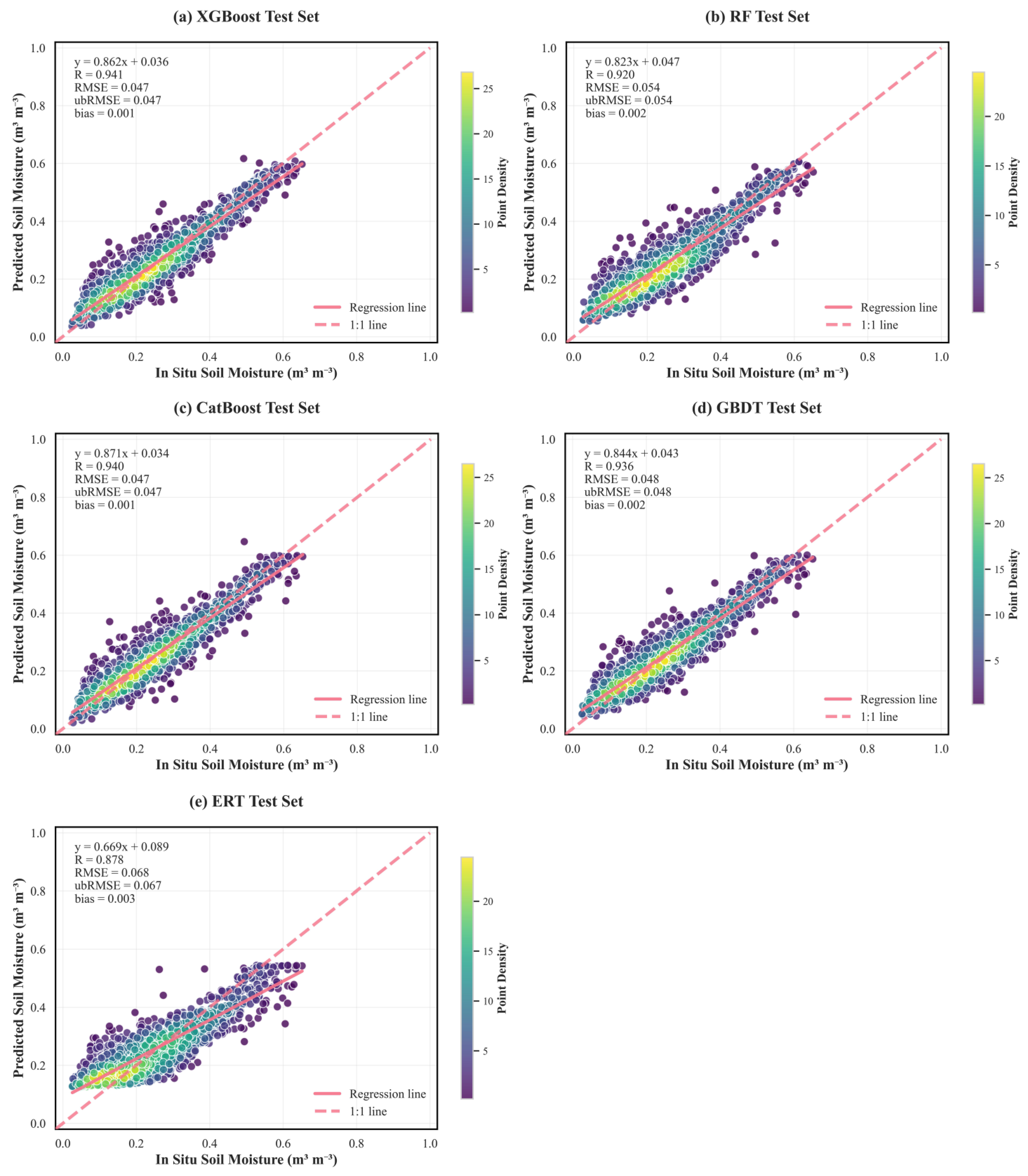
Based on the unfrozen period identified in Section 3.1, HLS data corresponding to each ground observation site were obtained, yielding a total of 4800 valid samples. These samples were split into training and validation sets with a 7:3 ratio. Five machine learning models—CatBoost, GBDT, ERT, RF, and XGBoost—were trained using 10-fold cross-validation. The results for all models on both training and test sets are presented as scatter plots in Figure 3. In the training set, except for the ERT model, all models achieved an R between predicted and observed soil moisture exceeding 0.98, with RMSE values less than 0.03. In the test set, the accuracy of each model declined to some extent, with R values ranging from 0.9 to 0.95. At this stage, the XGBoost model showed the highest accuracy, with an R of 0.941 and an RMSE of 0.047, making it the optimal upscaling model. The CatBoost model ranked second, with an R of 0.940 and an RMSE of 0.047.

The ERT model exhibits overestimation at low values and underestimation at high values, particularly in the soil moisture ranges of 0–0.15 and 0.5–0.6. This phenomenon is related to the feature selection strategy used by ERT during tree splitting. The ERT model randomly selects features and determines split thresholds, a mechanism that helps reduce overfitting but may increase bias, resulting in insufficient fitting in certain data intervals. Particularly in the low soil moisture range, limited training samples or uneven data distribution may hinder the model’s ability to represent the features in this region, leading to systematic underestimation. Additionally, ERT has relatively low sensitivity to extreme values, and its random splitting strategy may overlook fine-grained partitioning, further affecting prediction accuracy.

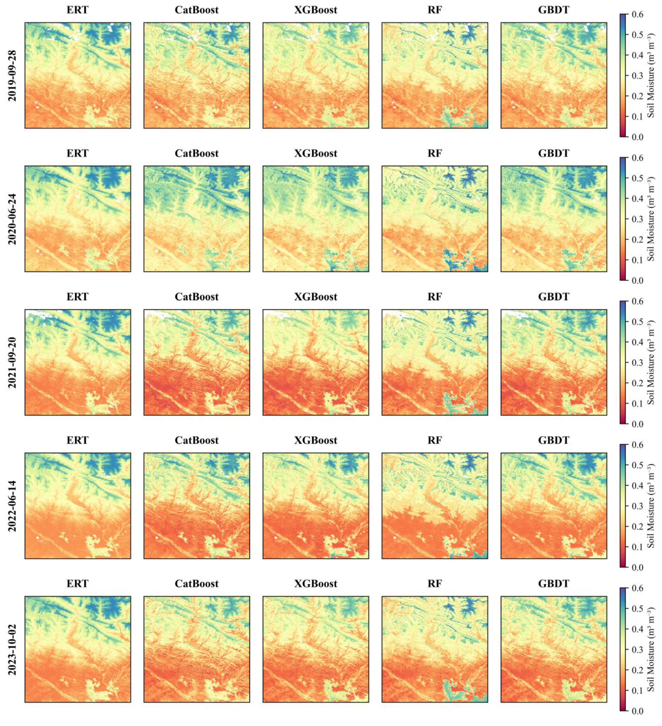
This study selected five remote sensing images from different years with minimal cloud cover to demonstrate the upscaled soil moisture distribution using machine learning models. Compared to traditional soil moisture reversion methods based on MODIS imagery, the 30-m resolution soil moisture products derived from HLS data more precisely and accurately capture the spatial heterogeneity of soil moisture in Tianjun. These products reveal detailed small-scale soil moisture variations while also depicting broader large-scale distribution patterns (see Figure 4). Overall, the spatial distribution of soil moisture exhibits a distinct pattern of drier conditions in the south and wetter conditions in the north. Moist areas are mainly concentrated in the northern alpine meadows and the extensive wetlands in the southeast, where flat terrain and water convergence contribute to higher soil moisture content. Specifically, the alpine meadows in the northeast are located at high elevations with relatively flat terrain, leading to substantial water accumulation and forming typical zones of high soil moisture. The wetland areas in the southeast are situated in relatively low terrain compared to the surrounding regions, acting as natural water collection zones that promote soil moisture accumulation. In the central mountainous area, a north–south-oriented belt of low soil moisture is evident; these zones largely consist of rock outcrop, weathered gravel and shallow soil layers, while the southern river valley area is primarily covered by sandy fluvial sediments, markedly limiting soil moisture retention capacity.

In the comparative analysis of different machine learning models, the ERT model’s soil moisture retrievals were overly smoothed and lacked sensitivity to inter-pixel variability, making it difficult to accurately capture subtle local variations in soil moisture. The CatBoost model demonstrated strong recognition abilities in both high- and low-moisture areas; however, it underestimated soil moisture in the wet region located in the lower-right corner of the study area, possibly due to the unique terrain or vegetation characteristics of that zone. The XGBoost model exhibited relatively stable performance, without significant overestimation or underestimation. The Random Forest (RF) model showed weaker capability in identifying north–south-aligned anthropogenic impervious surfaces, which may be related to the model’s limited ability to capture complex topographic influences, thereby restricting its prediction accuracy in these areas. The GBDT model produced relatively smooth soil moisture estimates in the high-elevation northeastern region, with limited spatial recognition, indicating that its model accuracy in high-elevation areas still needs improvement.

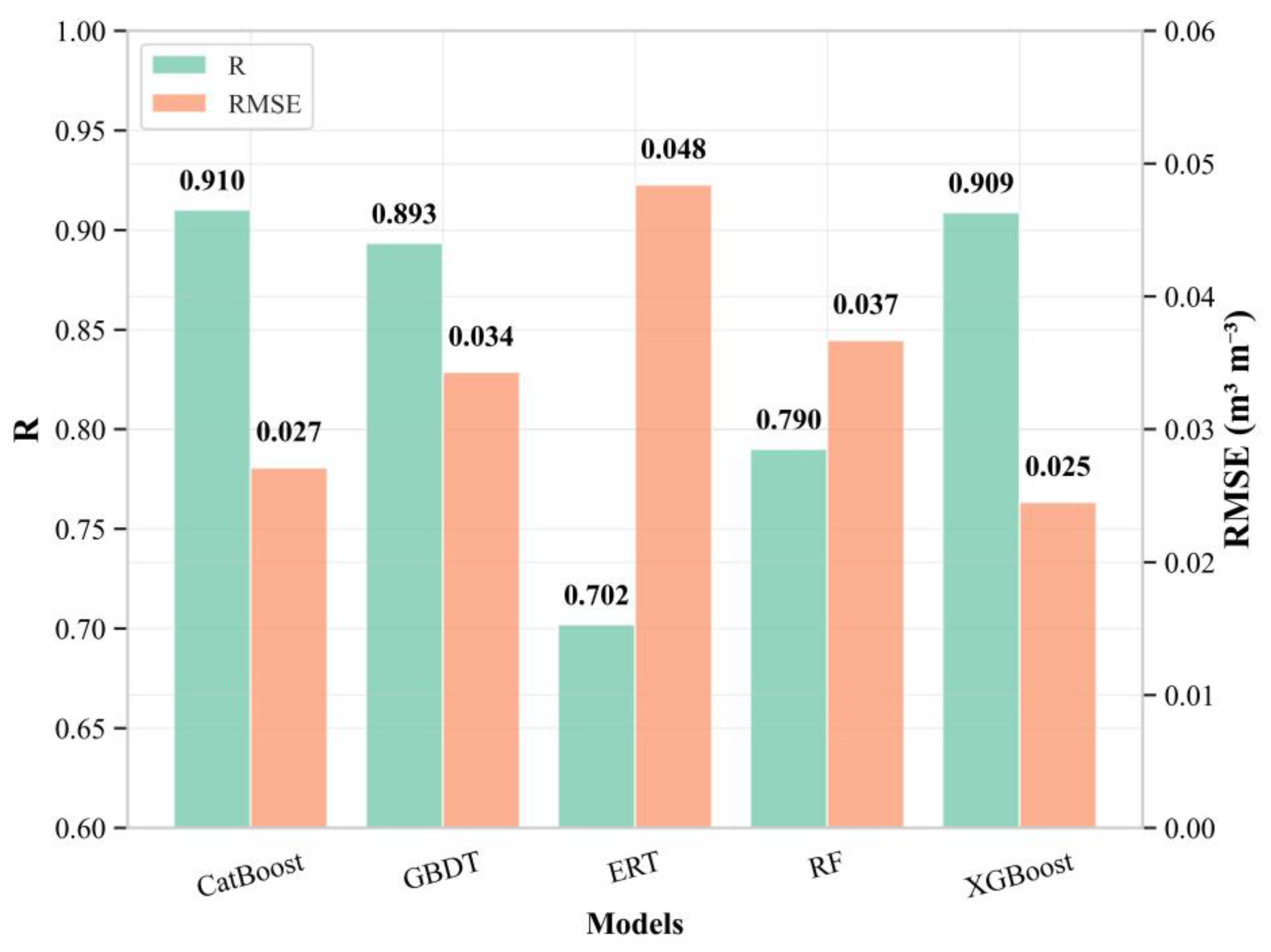
Based on the research by Chai et al. [23], the soil moisture sites of QLB-NET are relatively dense. As the number of sites used for averaging increases, the range between the upper and lower quartiles narrows. Average values can serve as the true soil moisture at the SMAP pixel scale for validation purposes. To further assess the differences among the various models, five upscaling models were applied to retrieve soil moisture from imagery covering over 90% of the study area. The resulting 30-m soil moisture values were then averaged within the SMAP pixel extent for comparison with the in situ average soil moisture. The accuracy metrics between the soil moisture averages from each upscaling model and the in situ soil moisture averages are presented in

Table 2. Accuracy metrics of soil moisture predictions for different machine learning Models.

Model	R	RMSE (m3 m−3)
CatBoost	0.910	0.027
GBDT	0.893	0.034
ERT	0.702	0.048
RF	0.790	0.037
XGBoost	0.909	0.025

and Figure 5, which display the same results in tabular and graphical form, respectively. It can be seen that both CatBoost and XGBoost performed well. The CatBoost model achieved the highest correlation with the in situ average soil moisture, with a coefficient of 0.910, while XGBoost had a correlation of 0.909. However, its RMSE was lower than that of CatBoost. The poorest performance was observed for the ERT model, with a correlation coefficient of only 0.702. Considering both R and RMSE, XGBoost was selected as the optimal upscaling model for soil moisture, and its results were compared with SMAP data to evaluate the applicability of SMAP soil moisture products in the study area.

3.3. SHAP

The SHAP method can comprehensively assess the influence of each feature on the predicted variable. Figure 6 illustrates the combined contribution and directional effect of different features on soil moisture prediction. The height of each bar represents the mean absolute SHAP value, reflecting the importance of each feature, while each point corresponds to a sample, with colors ranging from blue to red indicating low to high feature values, thereby revealing the direction and magnitude of each feature’s effect on soil moisture across different samples. The results show that elevation, sin_Doy, SWCI, swir2, and slope are the five features with significantly greater influence on soil moisture than others. The high SHAP values of sin_Doy clearly reflect the seasonal variation of soil moisture in the QLB-NET region, highlighting the critical role of seasonal periodicity in soil moisture dynamics. In terms of feature-specific influence, elevation, sin_Doy, and SWCI are generally positively correlated with soil moisture, meaning that higher values of these features correspond to greater soil moisture; in contrast, SWIR2 is negatively correlated with soil moisture. The effect of slope is more complex. Elevation is identified as a key driver of soil moisture in the QLB-NET region, manifested as moisture enrichment in both low- and high-elevation areas, with lower moisture levels observed in mid-elevation zones. The higher soil moisture at high elevations may result from lower temperatures and reduced evapotranspiration with increasing altitude, as well as the presence of flat terrain in the northern high mountain area that facilitates soil moisture retention. It should be mentioned here that this phenomenon is not common but exists in the highly heterogeneous mountain area. As a seasonal indicator, sin_Doy reflects the cyclical climatic controls on soil moisture status. The positive correlation between SWCI and soil moisture arises from its calculation, which leverages the strong absorption of water in two shortwave infrared bands. Because liquid water absorbs more strongly in swir2 than in swir1 [37], the reflectance of both bands decreases with increasing soil moisture, but the decrease is more pronounced in SWIR2. Consequently, higher SWCI values indicate higher surface soil moisture, which also explains the negative correlation between swir2 and soil moisture. Slope, as an important topographic variable, likely negatively affects soil moisture by increasing surface runoff and water loss; although its specific impact varies with local terrain and hydrological conditions, it contributes significantly to model predictions.

In summary, the SHAP analysis quantitatively reveals the influence and directional effects of each feature on soil moisture, providing scientific insight into the spatiotemporal variability of soil moisture in the QLB-NET region and serving as a reference for subsequent analyses.

3.4. SMAP Validation

Based on the previously selected XGBoost model for upscaling, with its soil moisture estimates regarded as ground truth, we validated both the 9 km resolution SPL3SMP_E product and the 36 km resolution SPL3SMP product. Significant differences in accuracy were observed between the two products, which are discussed in detail in the following sections.

3.4.1. Validation of SPL3SMP

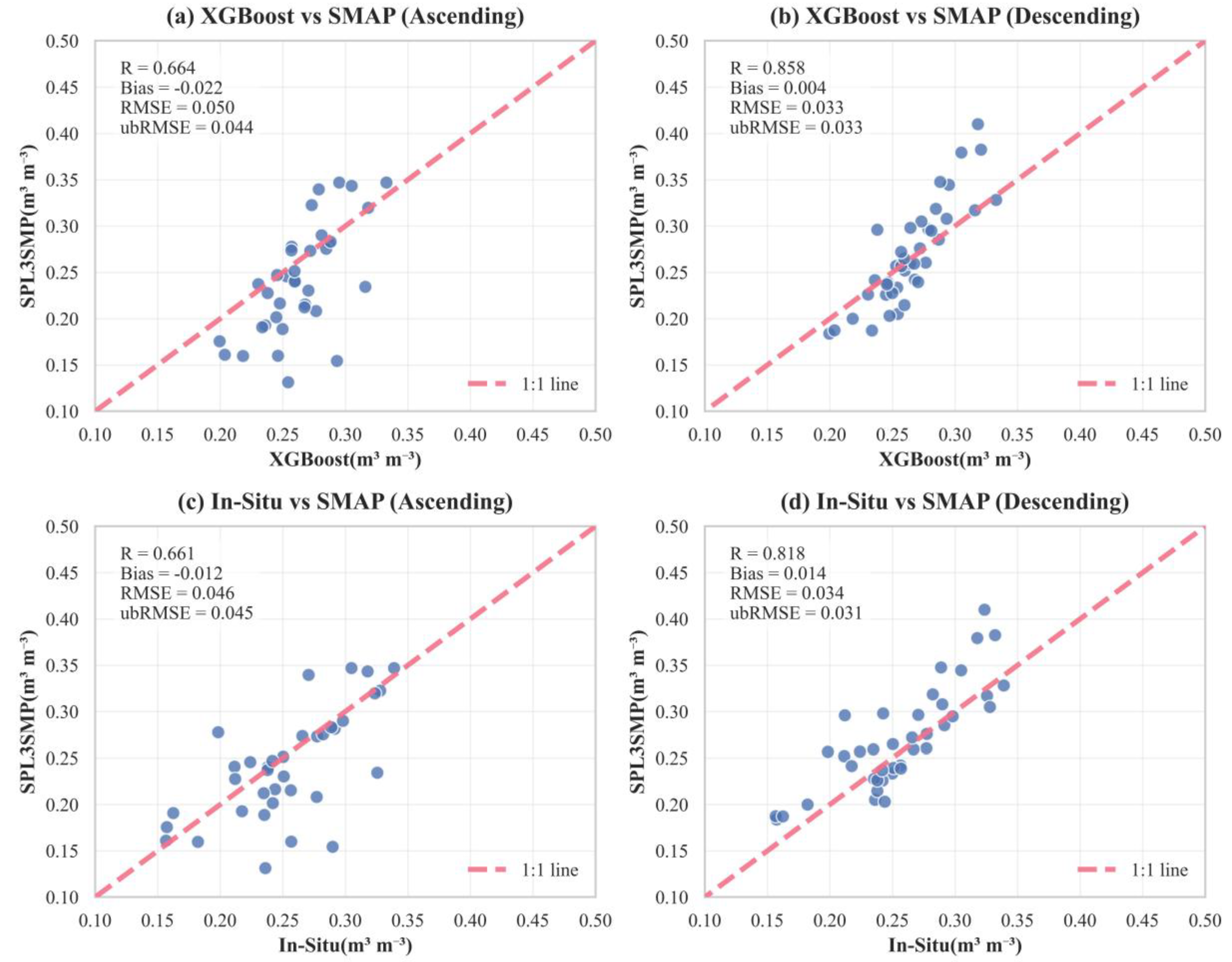
Figure 7 illustrates the accuracy of the SPL3SMP soil moisture product in the QLB-NET region. Compared with the ascending-orbit data, the descending-orbit data exhibit higher accuracy and meet the scientific observation requirement (ubRMSE ≤ 0.04 m³ m⁻³) [38], consistent with the findings of Chai et al. [23], further supporting the fact that observation performance varies significantly between different orbits. As shown in Figure 7b,d, the SPL3SMP data exhibit higher correlation with the XGBoost-upscaled average (r = 0.858) than with the in situ-measured average (r = 0.818). This result indicates that the XGBoost algorithm effectively bridges the scale gap between remote sensing retrievals and ground measurements, helping to reduce systematic biases caused by spatial representativeness mismatches.

Moreover, the SPL3SMP data show a pronounced orbit-dependent bias: descending-orbit data generally overestimate soil moisture, whereas ascending-orbit data systematically underestimate it. This pattern is likely related to differences in surface thermodynamic conditions at different overpass times. In the QLB-NET region, the ascending orbit occurs around 06:00 local time. With nocturnal solar radiation having ceased during the night, evapotranspiration is reduced, resulting in a relatively small decrease in soil moisture. Additionally, a lower land surface temperature (LST) can affect SMAP soil moisture retrievals [39], resulting in SMAP being lower than the soil moisture pixel “true” values. In contrast, the descending orbit occurs around 18:00 local time, when daytime evapotranspiration has reduced surface soil moisture, while SMAP retrievals—affected by surface temperature, moisture gradients, and radiative properties—tend to be higher than the pixel-scale “true” soil moisture values. The diurnal redistribution of soil moisture and the associated thermal dynamics likely constitute a key mechanism driving these orbit-dependent biases.

3.4.2. Validation of SPL3SMP_E

Table 3. Accuracy metrics between 9 km soil moisture and SMAP products.

Grid ID	Ascending				Grid ID	Descending
	R	Bias	RMSE	ubRMSE		R	Bias	RMSE	ubRMSE
1	0.797	−0.102	0.109	0.039	1	0.816	−0.072	0.081	0.036
2	0.663	−0.075	0.087	0.044	2	0.814	−0.046	0.059	0.036
3	0.702	−0.093	0.102	0.043	3	0.793	−0.066	0.075	0.035
4	0.389	−0.097	0.110	0.053	4	0.524	−0.070	0.082	0.043
5	0.773	−0.076	0.085	0.040	5	0.803	−0.048	0.060	0.036
6	0.717	−0.032	0.052	0.040	6	0.819	−0.007	0.035	0.034
7	0.702	−0.063	0.075	0.040	7	0.831	−0.039	0.050	0.032
8	0.692	−0.061	0.074	0.043	8	0.820	−0.040	0.052	0.034
9	0.638	0.045	0.064	0.046	9	0.808	0.066	0.076	0.038
10	0.693	0.030	0.050	0.040	10	0.802	0.051	0.063	0.037
11	0.756	0.031	0.048	0.037	11	0.852	0.052	0.062	0.033
12	0.780	0.027	0.046	0.037	12	0.873	0.044	0.055	0.032
13	0.735	0.057	0.070	0.041	13	0.853	0.076	0.083	0.034
14	0.770	0.054	0.066	0.037	14	0.873	0.076	0.083	0.034
15	0.856	0.023	0.038	0.031	15	0.876	0.043	0.054	0.033
16	0.814	0.041	0.053	0.035	16	0.914	0.055	0.064	0.031

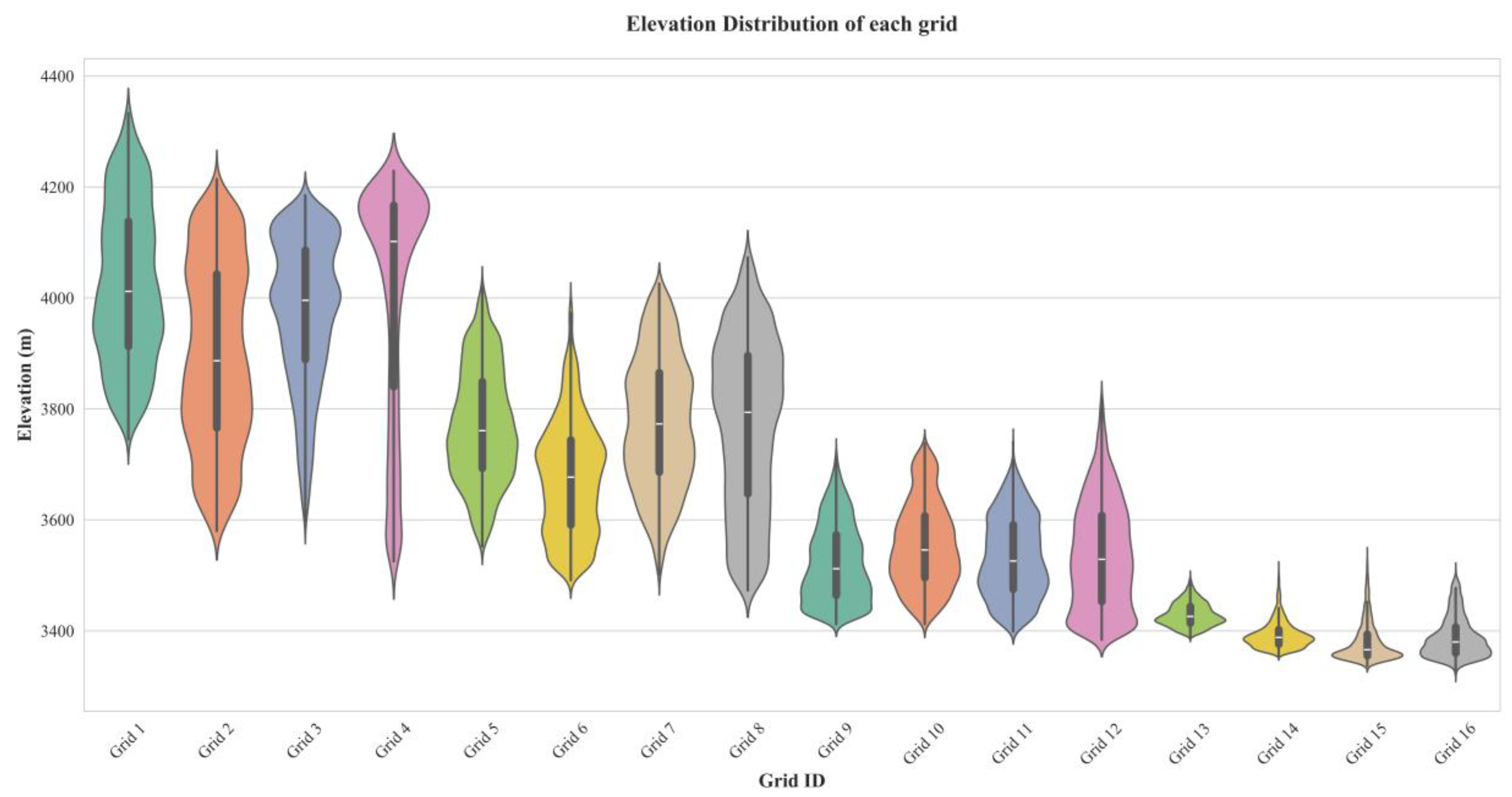
Note: The unit for bias, RMSE, and ubRMSE is m³ m⁻³.

presents the accuracy assessment of the SPL3SMP_E product in the QLB-NET region. The results indicate that descending-orbit data consistently outperform ascending-orbit data across all grids; 15 grids of descending-orbit data and 10 grids of ascending-orbit data meet the scientific observation requirement (ubRMSE ≤ 0.04m³ m⁻³) [38]. Significant spatial heterogeneity still exists among different geographic grids, which, according to Wu et al. [40], is mainly caused by elevation.

The violin plots of elevation distribution in Figure 8 provide intuitive support for this inference, clearly illustrating the variability of topographic characteristics within each grid. For instance, Grid 4 exhibits the most pronounced topographic fluctuations—reflected in its extremely narrow and elongated violin shape—which correspond directly to the lowest R. This strongly suggests that local terrain heterogeneity is a critical factor contributing to reduced satellite data accuracy.

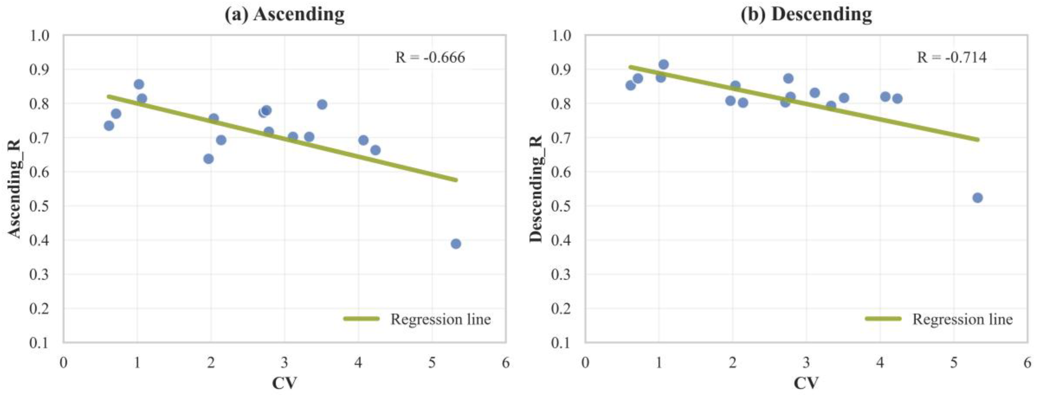
To quantitatively characterize such heterogeneity, this study employs the coefficient of variation (CV) of elevation as an objective measure of intra-grid terrain complexity. A larger CV indicates higher terrain complexity and stronger spatial heterogeneity. As a dimensionless measure of relative dispersion, CV effectively eliminates the scale effects caused by differences in mean elevation among grids, thereby providing a more intrinsic description of topographic variability. This establishes the foundation for systematically examining the quantitative relationship between terrain heterogeneity and SMAP data accuracy.

As shown in Figure 9, the elevation CV exhibits a clear negative correlation with the validation accuracy of the SMAP product, indicating that satellite retrieval accuracy decreases significantly as intra-grid topographic heterogeneity increases. However, this overall trend does not fully account for the accuracy differences observed across all grids. For instance, both Grid 2 and Grid 4 belong to high-heterogeneity areas (CV values of 4.23 and 5.32, respectively), yet their validation accuracies against XGBoost pixel “true” values differ substantially (descending-orbit R values of 0.814 and 0.524, respectively). The primary reason for this discrepancy is the insufficient spatial representativeness of stations within Grid 4: the stations are mainly concentrated in the southeastern part of the grid, while the high-altitude areas within the grid are difficult to access, resulting in a lack of adequate ground observations during station deployment. This uneven distribution leads to insufficient coverage of terrain variability, causing systematic biases in the “true” values generated by the XGBoost model for Grid 4, consequently reducing their agreement with the SMAP data. Therefore, in regions of extreme heterogeneity, validation accuracy depends not only on the performance of satellite retrievals but also heavily on the representativeness of ground stations relative to the underlying spatial heterogeneity.

In summary, the performance differences between the two products underscore the importance of accounting for spatial heterogeneity in soil moisture studies. Selecting an appropriate spatial resolution should consider terrain complexity and research objectives, balancing the need for accuracy with spatial detail. Future research could focus on integrating multi-resolution products to combine the strengths of both fine- and coarse-scale data, thereby enhancing the robustness and reliability of soil moisture estimation.

4. Discussion

This study employed Harmonized Landsat and Sentinel-2 (HLS v2.0) data to upscale soil moisture to a spatial resolution of 30 m. Unlike MODIS and Landsat data, which suffer from either coarse spatial resolution or limited temporal coverage, HLS v2.0 integrates Sentinel-2 and Landsat observations, thereby achieving both high spatial resolution and an improved temporal resolution with a median revisit interval of 2.9 days. This integration substantially enhances the applicability of optical remote sensing in mountainous and cloud-prone regions. Compared with the 570 samples obtained solely from Landsat data in the study by Wu et al. [40], the adoption of HLS v2.0 in this research yielded 4800 samples in the QLB-NET region—representing an approximately eightfold increase in sample size. Building upon this enriched dataset, high-resolution soil moisture upscaling over heterogeneous underlying surfaces was successfully achieved, and the applicability of SMAP products in the QLB-NET region was comprehensively evaluated.

Using the SHAP method, this study thoroughly examined the influence of various factors on soil moisture. In contrast to traditional feature importance metrics, SHAP not only quantifies the relative importance of each variable but also reveals the direction of their influence on the prediction results. Elevation was identified as the most important factor affecting soil moisture, with the spatial heterogeneity of the QLB-NET region largely driven by topographic variation. There is a general tendency for higher soil moisture in high-elevation areas and lower soil moisture in low-elevation areas. Elevation influences soil water storage by regulating temperature, precipitation, evaporation, and other environmental processes. In high-elevation alpine meadows, reduced evaporation and runoff promote water accumulation, leading to areas of high soil moisture. However, it is important to note that the influence of elevation on soil moisture is not universally applicable. Its effect is most pronounced in regions with distinct vertical zonation and substantial elevation differences; for example, in QLB-NET, the vertical range reaches up to 1042 m. In other regions, soil moisture at higher elevations may be lower than at lower elevations because water naturally flows toward depressions. This phenomenon is also observed in the southeastern wetland areas of QLB-NET, where lower elevations and minimal vertical differences facilitate water accumulation. Therefore, the relationship between elevation and soil moisture observed in this study is context-dependent, and its applicability and limitations vary with the scale of the study. These factors should be carefully considered in subsequent discussions and applications to ensure the accuracy and reliability of the conclusions. In addition, the day of year (DOY) was also identified as a key predictor. Figure 10 shows the model performance on the validation set with and without DOY as an input variable. It is evident that omitting DOY leads to a decline in accuracy across all models. Specifically, for the XGBoost model, incorporating DOY resulted in a 22.03% improvement in RMSE and a 4.3% increase in R. In contrast, the ERT model showed minimal change in accuracy regardless of whether DOY was included, which may be attributed to its high degree of randomness. Therefore, selecting appropriate input variables should be tailored to the characteristics of each model. These results indicate that incorporating temporal variables into the model is reasonable and effective for capturing the seasonal dynamics of soil moisture. The inclusion of temporal information also improves the model’s ability to detect anomalies caused by cloud cover or signal interference and to adjust predictions accordingly. The importance of DOY is consistent with findings reported by Shangguan et al. [41].

In evaluating the applicability of SMAP data in this region, for dates lacking ascending- or descending-orbit observations, this study filled the gaps by averaging SMAP data from the preceding and following days. This approach may introduce some errors, thereby reducing validation accuracy. A greater source of uncertainty arises from the impact of topographic heterogeneity on the reliability of pixel-level “ground truth.” The pixel-level “ground truth” generated through the XGBoost-based upscaling approach is highly dependent on the spatial representativeness of the ground stations used during model training. In areas with complex terrain (e.g., Grid 4), the dominant landform is high-altitude plains. However, due to harsh natural conditions and limited accessibility, researchers are unable to establish ground observation stations within this region. The existing stations, Stations 49 and 55, provide only limited spatial coverage and thus fail to adequately capture the pronounced topographic heterogeneity of the area. As a result, the model is forced to extrapolate extensively, which may lead to systematic biases in the upscaled results [42]. Therefore, the observed low correlation essentially reflects a comparison between SMAP pixel values and a pixel-level “ground truth” that itself suffers from uncertainties due to insufficient station representativeness. Although this limitation reduces the absolute accuracy of SMAP validation in such grids, it also highlights the diagnostic value of our approach: by identifying areas like Grid 4 as “failure zones” under the current validation scheme, our method provides actionable guidance for future observational network design. Increasing the density and representativeness of ground stations in these regions would substantially improve the reliability of both upscaled soil moisture and SMAP product evaluation. This discussion illustrates a broader implication of our study: even in areas with sparse ground data, machine learning-based upscaling can identify critical gaps and guide practical improvements in satellite product validation, emphasizing the method’s utility despite inherent uncertainties.

Soil properties, such as texture and organic matter content, strongly influence soil water holding capacity. However, due to the low spatial resolution of the available soil data, high-resolution soil property maps were not included in this study, which may limit the model’s accuracy at local scales. Future work could integrate high-precision soil data to improve both model performance and interpretability.

In addition, mixed pixel effects may influence soil moisture estimates derived from vegetation indices, as a single pixel can contain both green vegetation and bare soil, each contributing differently to reflectance. Such heterogeneity may cause over- or underestimation of soil moisture [43,44,45], particularly in areas with patchy vegetation or sparse cover. Despite these potential sources of uncertainty, our model remains effective. SHAP analysis indicates that predictions are primarily driven by elevation, day of year (DOY), SWIR reflectance, and the SWCI index, rather than relying solely on vegetation greenness. These variables provide complementary information that reflects both soil and vegetation conditions, enabling the model to capture large-scale soil moisture patterns reliably even in the presence of mixed pixels.

The machine learning approach adopted in this study is essentially data-driven and lacks explicit representation of underlying physical mechanisms. Although HLS data demonstrated good applicability in the QLB-NET region, its suitability for other regions remains to be further investigated. The predictive variables used in this study were relatively limited, which may not fully capture the diversity of factors influencing soil moisture. For SMAP validation, a direct aggregation approach was employed, whereby 30 m soil moisture estimates were averaged to match the 9 km and 36 km SMAP grids. This approach reduced errors compared with traditional point-based averaging, but uncertainties still exist. Future research directions may consider the following aspects:

• Integrating multi-source remote sensing datasets, such as microwave remote sensing, optical data, high-resolution soil dataset, and meteorological reanalysis products [46,47,48], to incorporate a more comprehensive set of predictors that reflect diverse environmental controls on soil moisture;
• Combining data-driven models with physical constraints, such as hydrological process models [49,50] or energy balance equations [51,52], to enhance model interpretability and robustness by providing physical meaning to the predictions;
• Expanding the analysis to multiple heterogeneous regions to systematically assess the applicability and generalization capability of SMAP and related models under complex terrain and variable environmental conditions [53,54,55];
• Paying attention to spectral mixing effects in optical remote sensing and exploring novel spectral unmixing algorithms in future studies to more accurately separate signals from vegetation, bare soil, and dry/dead vegetation, thereby improving soil moisture estimation in mixed pixels [56].

5. Conclusions

This study set out to develop and implement a robust methodology for upscaling soil moisture and validating SMAP satellite products over the highly heterogeneous landscape of the Qinghai–Tibet Plateau. Based on the comprehensive analysis conducted, we have successfully met our research objectives and drawn the following main conclusions:

• A diverse set of predictor variables was constructed from high-spatiotemporal-resolution HLS v2.0 data. When integrated with in situ measurements, these variables enabled multiple machine learning models to upscale soil moisture at a 30 m resolution, capturing significant fine-scale spatial heterogeneity within the study area.
• Among all models, XGBoost offered the highest predictive accuracy on the independent test set (R = 0.941, RMSE = 0.047 m³·m⁻³). The model’s strong performance is likely attributable to its ability to capture the complex, nonlinear relationships driven by factors such as elevation and seasonal dynamics (DOY).
• The high-resolution soil moisture product upscaled by the XGBoost model served as an effective pixel-scale validation reference. Its application helped mitigate errors from scale mismatch and spatial representativeness, improving the correlation with the 36 km SMAP product from R = 0.818 (using traditional in situ averaging) to R = 0.858.
• The validation provided further insights into SMAP’s performance in this region. Descending-orbit data generally yielded higher accuracy than ascending-orbit data, with only the 36 km descending-orbit product approaching the scientific standard. Moreover, the assessment of the 9 km product revealed a strong negative correlation between SMAP’s accuracy and terrain heterogeneity, highlighting potential challenges for the product in complex mountain environments.

References

1. Dubois, P.C.; Van Zyl, J.; Engman, T. Measuring Soil Moisture with Imaging Radars. IEEE Trans. Geosci. Remote Sens. 1995, 33, 915–926. [Google Scholar] [CrossRef]
2. Walker, J.; Rowntree, P.R. The Effect of Soil Moisture on Circulation and Rainfall in a Tropical Model. Quart. J. Royal Meteorol. Soc. 1977, 103, 29–46. [Google Scholar] [CrossRef]
3. Wood, E.F. Effects of Soil Moisture Aggregation on Surface Evaporative Fluxes. J. Hydrol. 1997, 190, 397–412. [Google Scholar] [CrossRef]
4. McColl, K.A.; Alemohammad, S.H.; Akbar, R.; Konings, A.G.; Yueh, S.; Entekhabi, D. The Global Distribution and Dynamics of Surface Soil Moisture. Nat. Geosci. 2017, 10, 100–104. [Google Scholar] [CrossRef]
5. Njoku, E.G.; Li, L. Retrieval of Land Surface Parameters Using Passive Microwave Measurements at 6-18 GHz. IEEE Trans. Geosci. Remote Sens. 1999, 37, 79–93. [Google Scholar] [CrossRef]
6. Owe, M.; De Jeu, R.; Holmes, T. Multisensor Historical Climatology of Satellite-derived Global Land Surface Moisture. J. Geophys. Res. 2008, 113, F01002. [Google Scholar] [CrossRef]
7. Koike, T.; Nakamura, Y.; Kaihotsu, I.; Davaa, G.; Matsuura, N.; Tamagawa, K.; Fujii, H. Development of an advanced microwave scanning radiometer (amsr-e) algorithm for soil moisture and vegetation water content. Proc. Hydraul. Eng. 2004, 48, 217–222. [Google Scholar] [CrossRef]
8. Kerr, Y.H.; Waldteufel, P.; Wigneron, J.-P.; Delwart, S.; Cabot, F.; Boutin, J.; Escorihuela, M.-J.; Font, J.; Reul, N.; Gruhier, C.; et al. The SMOS Mission: New Tool for Monitoring Key Elements Ofthe Global Water Cycle. Proc. IEEE 2010, 98, 666–687. [Google Scholar] [CrossRef]
9. Brocca, L.; Hasenauer, S.; Lacava, T.; Melone, F.; Moramarco, T.; Wagner, W.; Dorigo, W.; Matgen, P.; Martínez-Fernández, J.; Llorens, P.; et al. Soil Moisture Estimation through ASCAT and AMSR-E Sensors: An Intercomparison and Validation Study across Europe. Remote Sens. Environ. 2011, 115, 3390–3408. [Google Scholar] [CrossRef]
10. Zhao, L.; Yang, K.; Qin, J.; Chen, Y.; Tang, W.; Montzka, C.; Wu, H.; Lin, C.; Han, M.; Vereecken, H. Spatiotemporal Analysis of Soil Moisture Observations within a Tibetan Mesoscale Area and Its Implication to Regional Soil Moisture Measurements. J. Hydrol. 2013, 482, 92–104. [Google Scholar] [CrossRef]
11. Loew, A.; Schlenz, F. A Dynamic Approach for Evaluating Coarse Scale Satellite Soil Moisture Products. Hydrol. Earth Syst. Sci. 2011, 15, 75–90. [Google Scholar] [CrossRef]
12. Kang, J.; Jin, R.; Li, X. Regression Kriging-Based Upscaling of Soil Moisture Measurements From a Wireless Sensor Network and Multiresource Remote Sensing Information Over Heterogeneous Cropland. IEEE Geosci. Remote Sens. Lett. 2015, 12, 92–96. [Google Scholar] [CrossRef]
13. Wang, J.; Ge, Y.; Song, Y.; Li, X. A Geostatistical Approach to Upscale Soil Moisture With Unequal Precision Observations. IEEE Geosci. Remote Sens. Lett. 2014, 11, 2125–2129. [Google Scholar] [CrossRef]
14. Qin, J.; Yang, K.; Lu, N.; Chen, Y.; Zhao, L.; Han, M. Spatial Upscaling of In-Situ Soil Moisture Measurements Based on MODIS-Derived Apparent Thermal Inertia. Remote Sens. Environ. 2013, 138, 1–9. [Google Scholar] [CrossRef]
15. Chen, J.; Hu, F.; Li, J.; Xie, Y.; Zhang, W.; Huang, C.; Meng, L. Evaluation of SMAP-Enhanced Products Using Upscaled Soil Moisture Data Based on Random Forest Regression: A Case Study of the Qinghai–Tibet Plateau, China. ISPRS Int. J. Geo-Inf. 2023, 12, 281. [Google Scholar] [CrossRef]
16. Xu, J.; Su, Q.; Li, X.; Ma, J.; Song, W.; Zhang, L.; Su, X. A Spatial Downscaling Framework for SMAP Soil Moisture Based on Stacking Strategy. Remote Sens. 2024, 16, 200. [Google Scholar] [CrossRef]
17. Long, D.; Bai, L.; Yan, L.; Zhang, C.; Yang, W.; Lei, H.; Quan, J.; Meng, X.; Shi, C. Generation of Spatially Complete and Daily Continuous Surface Soil Moisture of High Spatial Resolution. Remote Sens. Environ. 2019, 233, 111364. [Google Scholar] [CrossRef]
18. Zheng, G.; Zhao, T.; Liu, Y. Cloud Removal in the Tibetan Plateau Region Based on Self-Attention and Local-Attention Models. Sensors 2024, 24, 7848. [Google Scholar] [CrossRef]
19. Chrysanthopoulos, E.; Kallioras, A. Temporal and Geographic Extrapolation of Soil Moisture Using Machine Learning Algorithms. CATENA 2025, 257, 109156. [Google Scholar] [CrossRef]
20. Ju, J.; Zhou, Q.; Freitag, B.; Roy, D.P.; Zhang, H.K.; Sridhar, M.; Mandel, J.; Arab, S.; Schmidt, G.; Crawford, C.J.; et al. The Harmonized Landsat and Sentinel-2 Version 2.0 Surface Reflectance Dataset. Remote Sens. Environ. 2025, 324, 114723. [Google Scholar] [CrossRef]
21. Roy, D.; Ghosh, T.; Das, B.; Jatav, R.; Chakraborty, D. Smartphone-Based Image Analysis and Interpretable Machine Learning for Soil Moisture Estimation across Diverse Indian Soils. Remote Sens. Appl. Soc. Environ. 2025, 39, 101655. [Google Scholar] [CrossRef]
22. Bayable, G.; Gebrie, G.; Melese, T.; Melaku, A. Land Use/Cover Classification Using Machine Learning Algorithms and Their Impacts on Land Surface Temperature and Soil Moisture in the Alawuha Watershed, Ethiopia. Environ. Sustain. Indic. 2025, 27, 100797. [Google Scholar] [CrossRef]
23. Chai, L.; Zhu, Z.; Liu, S.; Xu, Z.; Jin, R.; Li, X.; Kang, J.; Che, T.; Zhang, Y.; Zhang, J.; et al. QLB-NET: A Dense Soil Moisture and Freeze–Thaw Monitoring Network in the Qinghai Lake Basin on the Qinghai–Tibetan Plateau. Bull. Am. Meteorol. Soc. 2024, 105, 584–604. [Google Scholar] [CrossRef]
24. Uuemaa, E.; Ahi, S.; Montibeller, B.; Muru, M.; Kmoch, A. Vertical Accuracy of Freely Available Global Digital Elevation Models (ASTER, AW3D30, MERIT, TanDEM-X, SRTM, and NASADEM). Remote Sens. 2020, 12, 3482. [Google Scholar] [CrossRef]
25. Zhang, R.; Kim, S.; Sharma, A. A Comprehensive Validation of the SMAP Enhanced Level-3 Soil Moisture Product Using Ground Measurements over Varied Climates and Landscapes. Remote Sens. Environ. 2019, 223, 82–94. [Google Scholar] [CrossRef]
26. González-Ramírez, A.; Atzberger, C.; Torres-Roman, D.; López, J. Representation Learning of Multi-Spectral Earth Observation Time Series and Evaluation for Crop Type Classification. Remote Sens. 2025, 17, 378. [Google Scholar] [CrossRef]
27. Zhu, L.; Dai, J.; Liu, Y.; Yuan, S.; Qin, T.; Walker, J.P. A Cross-Resolution Transfer Learning Approach for Soil Moisture Retrieval from Sentinel-1 Using Limited Training Samples. Remote Sens. Environ. 2024, 301, 113944. [Google Scholar] [CrossRef]
28. Pedregosa, F.; Varoquaux, G.; Org, N.; Gramfort, A.; Gramfort, A.; Michel, V.; Michel, V.; Fr, L.; Thirion, B.; Thirion, B.; et al. Scikit-Learn: Machine Learning in Python. J. Mach. Learn. Res. 2011, 12, 2825–2830. [Google Scholar]
29. Zhou, Z.; Sun, O.J.; Luo, Z.; Jin, H.; Chen, Q.; Han, X. Variation in Small-Scale Spatial Heterogeneity of Soil Properties and Vegetation with Different Land Use in Semiarid Grassland Ecosystem. Plant Soil. 2008, 310, 103–112. [Google Scholar] [CrossRef]
30. Breiman, L. Random Forests. Mach. Learn. 2001, 45, 5–32. [Google Scholar] [CrossRef]
31. Geurts, P.; Ernst, D.; Wehenkel, L. Extremely Randomized Trees. Mach. Learn. 2006, 63, 3–42. [Google Scholar] [CrossRef]
32. Chen, T.; Guestrin, C. XGBoost: A Scalable Tree Boosting System. In Proceedings of the 22nd ACM Sigkdd International Conference on Knowledge Discovery and Data Mining, San Francisco, CA, USA, 13–17 August 2016. [Google Scholar] [CrossRef]
33. Prokhorenkova, L.; Gusev, G.; Vorobev, A.; Dorogush, A.V.; Gulin, A. CatBoost: Unbiased Boosting with Categorical Features. In Proceedings of the Advances in Neural Information Processing Systems, San Diego, CA, USA, 2–8 December 2018; Volume 31. [Google Scholar]
34. Friedman, J.H. Greedy Function Approximation: A Gradient Boosting Machine. Ann. Stat. 2001, 29, 1189–1232. [Google Scholar] [CrossRef]
35. Lundberg, S.; Lee, S.-I. A Unified Approach to Interpreting Model Predictions. In Proceedings of the Advances in Neural Information Processing Systems 30, Long Beach, CA, USA, 4–9 December 2017; Volume 30. [Google Scholar]
36. Pradhan, B.; Dikshit, A.; Lee, S.; Kim, H. An Explainable AI (XAI) Model for Landslide Susceptibility Modeling. Appl. Soft Comput. 2023, 142, 110324. [Google Scholar] [CrossRef]
37. Zhang, H. Hyperspectral Response Characteristics and Monitor on Soil Water. Crops 2023, 1, 233–238. [Google Scholar] [CrossRef]
38. Chan, S.; Bindlish, R.; Chaubell, M.; Colliander, A.; Chen, F.; Dunbar, S.; Jackson, T.; Cosh, M.; Bongiovanni, T.; Walker, J.; et al. Soil Moisture Active Passive (SMAP) Project: Calibration and Validation for the L2/3_SM_P Version 7 and L2/3_SM_P_E Version 4 Data Products; National Snow and Ice Data Center: Boulder, CO, USA, 2020. [Google Scholar]
39. Chen, Y.; Yang, K.; Qin, J.; Cui, Q.; Lu, H.; La, Z.; Han, M.; Tang, W. Evaluation of SMAP, SMOS, and AMSR2 Soil Moisture Retrievals against Observations from Two Networks on the Tibetan Plateau. JGR Atmos. 2017, 122, 5780–5792. [Google Scholar] [CrossRef]
40. Wu, Q.; Zhu, Z.; Ma, J.; Liu, S.; Chai, L.; Xu, Z. Soil Moisture Retrieval Based on Ensemble Learning Models Using Landsat8 Data in Areas of High Heterogeneity. ResearchGate 2024, in press. [Google Scholar] [CrossRef]
41. Shangguan, Y.; Min, X.; Shi, Z. Inter-Comparison and Integration of Different Soil Moisture Downscaling Methods over the Qinghai-Tibet Plateau. J. Hydrol. 2023, 617, 129014. [Google Scholar] [CrossRef]
42. Duan, X.; Maqsoom, A.; Khalil, U.; Aslam, B.; Amjad, T.; Tufail, R.F.; Alarifi, S.S.; Tariq, A. Enhancing Soil Moisture Retrieval in Semi-Arid Regions Using Machine Learning Algorithms and Remote Sensing Data. Appl. Soil. Ecol. 2024, 204, 105687. [Google Scholar] [CrossRef]
43. Burchard-Levine, V.; Nieto, H.; Riaño, D.; Migliavacca, M.; El-Madany, T.S.; Guzinski, R.; Carrara, A.; Martín, M.P. The Effect of Pixel Heterogeneity for Remote Sensing Based Retrievals of Evapotranspiration in a Semi-Arid Tree-Grass Ecosystem. Remote Sens. Environ. 2021, 260, 112440. [Google Scholar] [CrossRef]
44. Shen, M.; Tang, Y.; Chen, J.; Zhu, X.; Zheng, Y. Influences of Temperature and Precipitation before the Growing Season on Spring Phenology in Grasslands of the Central and Eastern Qinghai-Tibetan Plateau. Agric. For. Meteorol. 2011, 151, 1711–1722. [Google Scholar] [CrossRef]
45. Helman, D. Land Surface Phenology: What Do We Really ‘See’ from Space? Sci. Total Environ. 2018, 618, 665–673. [Google Scholar] [CrossRef] [PubMed]
46. He, L.; He, Z.; Chen, X.; Li, L.; Wu, W.; Kang, G.; Gong, J. Metallogenic Prediction Based on Multi-Source Remote Sensing and Machine Learning: A Case of Lithium Ore in Jiajika, China. Ore Geol. Rev. 2025, 185, 106813. [Google Scholar] [CrossRef]
47. Garcia-Prats, A.; Carricondo-Antón, J.M.; Ippolito, M.; De Caro, D.; Jiménez-Bello, M.A.; Manzano-Juárez, J.; Pulido-Velazquez, M. High-Resolution Spatially Interpolated FAO Penman-Monteith Crop Reference Evapotranspiration Maps of Sicily Island (Italy) and Jucar River System (Spain) Using AgERA5 and ERA5-Land Reanalysis Datasets. J. Hydrol. Reg. Stud. 2025, 60, 102531. [Google Scholar] [CrossRef] [PubMed]
48. Majidi, F.; Sabetghadam, S.; Gharaylou, M.; Rezaian, R. Evaluation of the Performance of ERA5, ERA5-Land and MERRA-2 Reanalysis to Estimate Snow Depth over a Mountainous Semi-Arid Region in Iran. J. Hydrol. Reg. Stud. 2025, 58, 102246. [Google Scholar] [CrossRef]
49. Fang, Z.; Qu, S.; Li, Z.; Li, Q.; Shi, P.; Sun, Y.; Yang, X.; Tang, H.; Zhang, J.; Zhu, Z.; et al. Soil Water Accounting Network (SWAN): A Novel Neural Network for Modeling Conceptual Hydrological Processes. J. Hydrol. 2025, 661, 133562. [Google Scholar] [CrossRef]
50. Fang, Q. Decoupling Climate and Vegetation Impacts on Hydrological Processes in Semi-Arid Regions Using an Improved Grid-Scale Budyko Model. J. Hydrol. Reg. Stud. 2025, 61, 102691. [Google Scholar] [CrossRef]
51. Zhao, C.; Guan, C.; Yu, T.; Wang, J.; Li, H.; Wang, X.; Zhang, B.; Kou, S.; Liu, X.; Zhao, C. Feasibility of Planting Shrubs in Arid Areas from a Water Balance Perspective. J. Hydrol. 2025, 661, 133753. [Google Scholar] [CrossRef]
52. Bai, X.; Fan, S.; Li, R.; Dai, T.; Li, W.; Ye, S.; Qian, L.; Liu, L.; Zhang, Z.; Chen, H.; et al. Estimating Root Zone Soil Moisture in Farmland by Integrating Multi-Source Remote Sensing Data Based on the Water Balance Equation. Agric. Water Manag. 2025, 314, 109544. [Google Scholar] [CrossRef]
53. Min, X.; Shangguan, Y.; Li, D.; Shi, Z. Improving the Fusion of Global Soil Moisture Datasets from SMAP, SMOS, ASCAT, and MERRA2 by Considering the Non-Zero Error Covariance. Int. J. Appl. Earth Obs. Geoinf. 2022, 113, 103016. [Google Scholar] [CrossRef]
54. Kim, H.; Crow, W.; Li, X.; Wagner, W.; Hahn, S.; Lakshmi, V. True Global Error Maps for SMAP, SMOS, and ASCAT Soil Moisture Data Based on Machine Learning and Triple Collocation Analysis. Remote Sens. Environ. 2023, 298, 113776. [Google Scholar] [CrossRef]
55. Hu, F.; Wei, Z.; Yang, X.; Xie, W.; Li, Y.; Cui, C.; Yang, B.; Tao, C.; Zhang, W.; Meng, L. Assessment of SMAP and SMOS Soil Moisture Products Using Triple Collocation Method over Inner Mongolia. J. Hydrol. Reg. Stud. 2022, 40, 101027. [Google Scholar] [CrossRef]
56. Chen, X.; Wang, D.; Chen, J.; Wang, C.; Shen, M. The Mixed Pixel Effect in Land Surface Phenology: A Simulation Study. Remote Sens. Environ. 2018, 211, 338–344. [Google Scholar] [CrossRef]
Figure 1. Study area location, elevation (NASADEM), and soil moisture site distribution.
Land 14 02098 g001
Figure 2. Time series variation in soil temperature and soil moisture in QLB-NET.
Land 14 02098 g002
Figure 3. Scatter plot of different machine learning models: (a) XGBoost on test set; (b) Random Forest on test set; (c) CatBoost on test set; (d) GBDT on test set; (e) ERT on test set.
Land 14 02098 g003
Figure 4. Spatial distribution of soil moisture from various models at 30 m spatial resolution.
Land 14 02098 g004
Figure 5. Comparison of R and RMSE across different machine learning models.
Land 14 02098 g005
Figure 6. SHAP explanation.
Land 14 02098 g006
Figure 7. Scatter plots of SPL3SMP ascending-orbit and descending-orbit data vs. XGBoost and in situ data. (a) XGBoost upscaling results vs. ascending-orbit data; (b) XGBoost upscaling results vs. descending-orbit data; (c) In situ measurement means vs. ascending-orbit data; (d) In situ measurement means vs. descending-orbit data.
Land 14 02098 g007
Figure 8. Elevation distribution of each grid.
Land 14 02098 g008
Figure 9. The effect of terrain heterogeneity on the correlation of SMAP soil moisture.
Land 14 02098 g009
Figure 10. Performance of five soil moisture upscaling algorithms with and without DOY information.
Land 14 02098 g010