Dynamic Spatiotemporal Evolution of Ecological Environment in the Yellow River Basin in 2000–2024 and the Driving Mechanisms

Abstract

The Yellow River Basin (YRB), a pivotal ecoregion in China, has long been plagued by a range of ecological problems, including water loss, soil erosion, and ecological degradation. Despite previous reports on the ecological environment of YRB, systematic studies on the multi-factor driving mechanism and the coupling between the ecological and hydrological systems remain scarce. In this study, with multi-source remote-sensing imagery and measured hydrological data, the random forest (RF) model and the geographical detector (GD) technique were employed to quantify the dynamic spatiotemporal changes in the ecological environment of YRB in 2000–2024 and identify the driving factors. The variables analyzed in this study included gross primary productivity (GPP), fractional vegetation cover (FVC), land use and cover change (LUCC), meteorological statistics, as well as runoff and sediment data measured at hydrological stations in YRB. The main findings are as follows: first, the GPP and FVC increased significantly by 37.9% and 18.0%, respectively, in YRB in 2000–2024; second, LUCC was the strongest driver of spatiotemporal changes in the ecological environment of YRB; third, precipitation and runoff contributed positively to vegetation growth, whereas the sediment played a contrary role, and the response of ecological variables to the hydrological processes exhibited a time lag of 1–2 years. This study is expected to provide scientific insights into ecological conservation and water resources management in YRB, and offer a decision-making basis for the design of sustainability policies and eco-restoration initiatives.

1. Introduction

The Yellow River Basin (YRB), the cradle of Chinese civilization and a key ecological zone in northern China [1], has long faced escalating ecological threats from climate change and intensified human activities, including severe soil erosion and ecosystem degradation [2,3,4]. Scientific interventions are required to resolve these challenges and balance ecological security protection with socio-economic development.

Globally, studies on ecological environmental dynamics have experienced three stages of development over the years: (1) Earlier research focused on the impacts of one specific single factor on the ecological environment or qualitative analyses of anthropogenic impacts [5,6,7], which often overlooked the complexity of the ecological environmental system. (2) Studies later utilized multi-source remote-sensing data to quantify the spatiotemporal evolution of key ecological indicators, such as the gross primary productivity (GPP)—a key indicator of ecosystem carbon cycling [8,9,10], and identify the key drivers of different landscapes [11,12]. (3) Recent studies incorporated carbon–water coupling analysis to unveil biogeochemical feedbacks [13,14] and assess the response of regional ecosystems to global changes through process-based ecosystem modeling [15,16,17]. The research methodologies in this domain have also advanced from traditional statistical analysis to machine learning frameworks [18,19] and physics constraint models; these models, by assimilating field observations with satellite data, increased the prediction accuracy of nonlinear ecological behaviors.

In this global context, research on the dynamic evolution of the ecological environment in YRB has made significant but unsystematic progress. Some pioneering studies identified the correlation between climate variables and vegetation dynamics, using the MODIS-derived products of GPP and fractional vegetation cover (FVC) to predict the greening trends across the basin in relation to global warming and eco-protection policies [18,20]. For instance, Lin et al. [21] examined the impacts of climate change on the water-carbon utilization efficiency in YRB by analyzing the trajectory of the normalized difference vegetation index (NDVI); Xue et al. [12] quantified the influence of extreme droughts on the vegetation productivity in the basin. Studies on the land use and land cover change (LUCC) in YRB investigated the mechanism underlying the transitions from natural ecological landscapes to urban land, and attributed these transitions to agricultural expansion and construction of hydraulic engineering projects [3,22,23]. Some hydrological studies in YRB measured the variations in the runoff and sediment flux in the upper, middle, and lower reaches of the basin, and identified the correlations between the sediment flux and erosion control challenges [3,24]. Despite these previous research efforts, limitations remain: (1) The low resolution of currently available datasets of YRB failed to reflect the regional heterogeneity in the Loess Plateau and other topographically complex areas, resulting in uncertainties in the inversion of GPP. (2) In previous works, the bi-directional feedback between the ecological variables and the hydrological processes was disregarded: though some examined the precipitation-runoff interactions [25,26], the lagged effects of sediments on vegetation recovery were not examined. (3) Though LUCC [22,23], climate [2], and hydrological factors were identified as the co-drivers for ecological environmental variations in YRB, quantitative evaluation of the interactions between these driving factors based on spatially explicit modeling was lacking; (4) the conflict between three staircase topography [24], vegetation gradient [27], and intensive human activities [3] in YRB has led to unique thresholds of ecological variations in the basin, but most prediction models failed to interpret the complex correlations between the variables involved [20,21,28,29,30,31,32].

The limitations specified above allowed us to identify the research direction on the macro-ecological environmental variations in YRB—to shift from unsystematic and correlation-based analyses to establishing a comprehensive ecological and hydrological framework that could quantify cross-scale correlations and mechanical driving factors. Specifically, the following challenges need to be addressed: (1) As the MODIS data (500 m^–1 km) [33,34,35,36,37,38,39] could not reflect the fine terrain–soil–vegetation correlations that are crucial to erosion slopes [27,32], topographical data with a higher resolution (such as 30 m ASTER DEM data) need to be incorporated. (2) Though the response of GPP to climate was modeled [20,21], the hydrological drivers were not integrated with carbon cycle assessment [8,13]. (3) The lagged response of the ecological environment to extreme hydrological events was disregarded in existing models [40], making these models not suitable for research in YRB due to the high risk of flood and drought events [2]. (4) The geo-detector (GD) technique [41,42,43,44] was not fully utilized in the analysis of driving factors (such as LUCC and precipitation) of ecological environmental evolution.

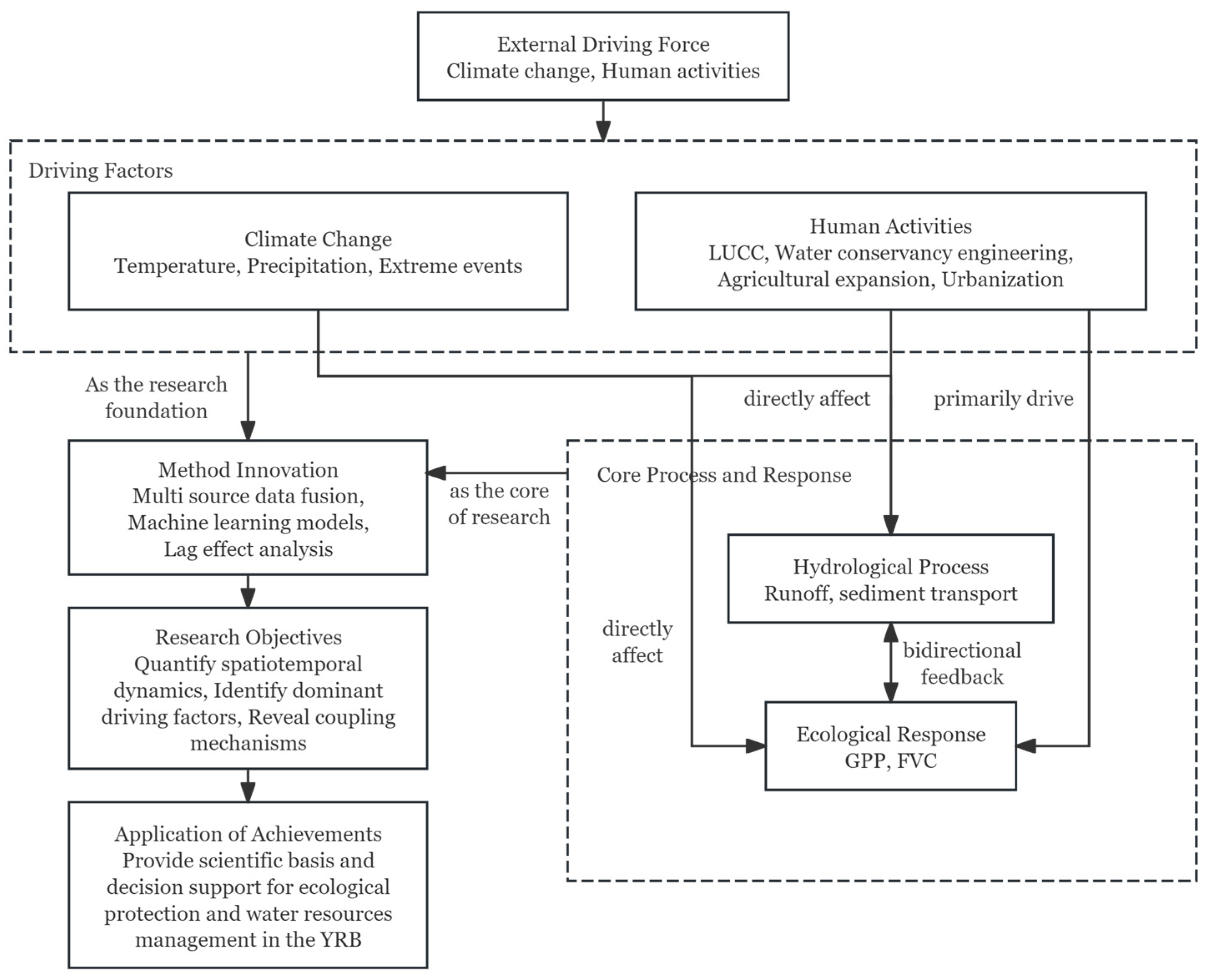
To address the systemic complexity and the research gaps identified above, we propose a conceptual framework (Figure 1) that illustrates the interplay between key drivers, processes, and responses within the YRB ecosystem. This research contributed to the existing literature through three innovations in methodology and theory: (1) The high-resolution topographic data (ASTER DEM), multi-temporal MODIS data (GPP: MOD17A3HGF; FVC: MOD13A1; LUCC: MCD12Q1) [33,34,35,36,37,38,39], and ground-validated hydrological records (2000–2024) for the study area were combined, which improved the spatiotemporal precision in characterizing the ecology–hydrology coupling relationship. (2) A dual-model framework was proposed: the random forest (RF) model, which ranked the driving factors, and the GD model, which portrayed the spatial heterogeneity, were combined to identify the interactions between LUCC, climate, topography, soil, and hydrological processes in the basin. (3) Cross-correlation analysis was performed to quantify the delayed response of GPP/FVC to the sediment flux, which could help accurately identify the recovery time of erosion hotspots in the basin. These innovations collectively resolved the biases of isolated mono-disciplinary research and provided a comprehensive understanding of the ecological evolution trajectories in YRB in the context of global changes.

2. Study Area and Data Sources

2.1. Study Area Overview

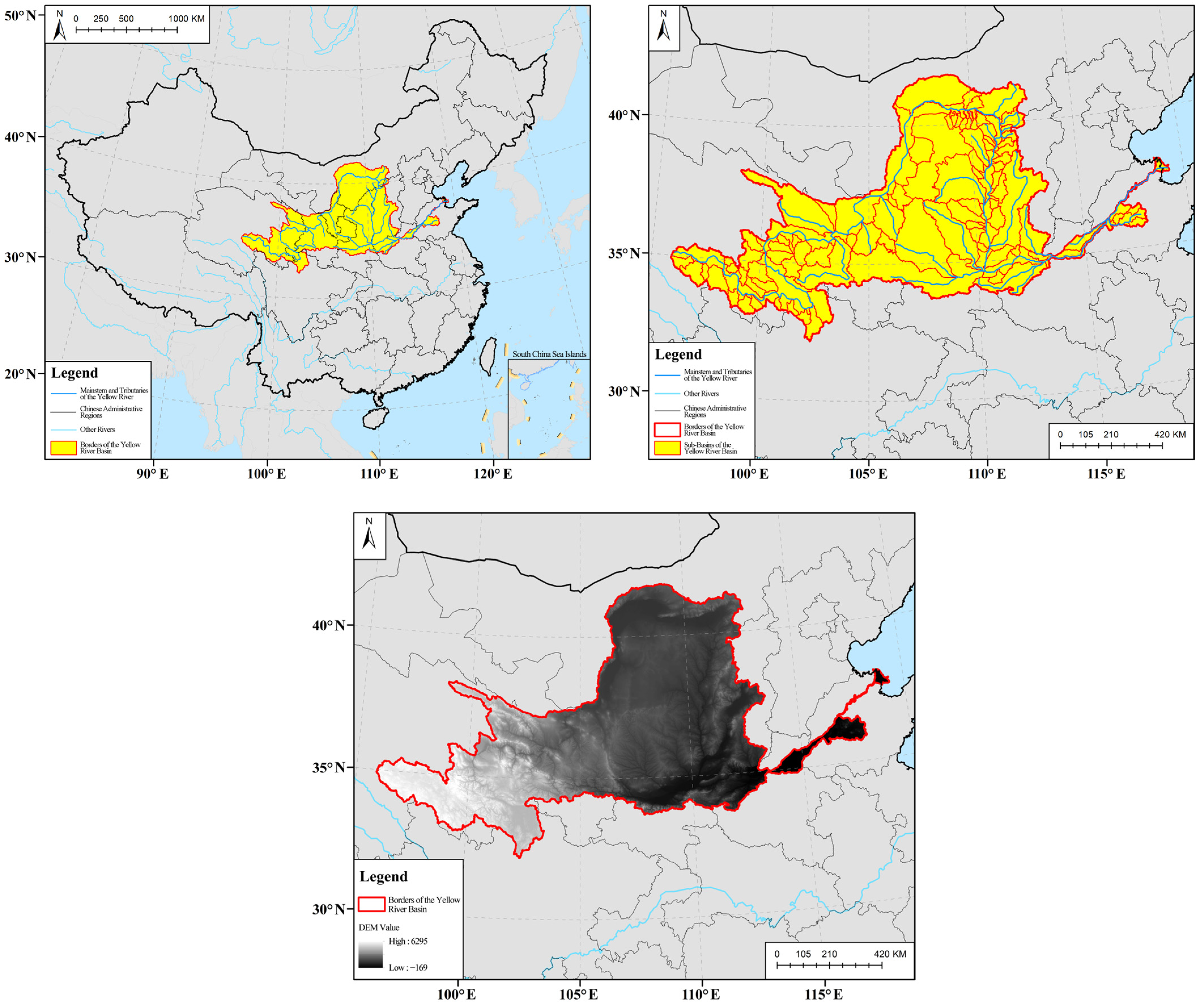
The Yellow River, originating from the Yoguzonglie Basin at the northern foot of Bayan Kara Mountain on the Qinghai–Tibet Plateau, stretches 5464 km eastwards through nine provinces, including Qinghai, Sichuan, Gansu, Ningxia, Inner Mongolia, Shanxi, Shaanxi, Henan, and Shandong, before joining the Bohai Sea in eastern China. The Yellow River Basin (YRB) (32°35′~41°49′ N; 95°10′~119°06′ E), covering an area of 795,000 km² (including an inland catchment of 42,000 km²), slopes downward from west to east with significant topographic variations; the basin demonstrates a three-step staircase-like terrain distribution, running across four geomorphic units—the Qinghai–Tibet Plateau, Inner Mongolia Plateau, Loess Plateau, and Huang-Huai-Hai Plain [24]. Subject to a continental climate, the basin has a semi-arid climate in its southeastern area, a semi-humid climate in its central region, and an arid climate in its northwestern part. The diverse landforms and complex habitats in the basin provide favorable conditions for vegetation growth [45], and from its southeast to its northwest, the basin is dominated by forest steppe, dry steppe, and desert steppe [27]. The topographic complexity, vegetation diversity, and substantial climatic differences across the YRB lead to a variety of ecosystems in the basin. Figure 2 shows the maps of the study area.

2.2. Data Sources

Multi-source remote-sensing imagery, measured hydrological data, and other spatial data were collected to analyze the spatiotemporal evolution of the ecological environment in YRB and identify the impacts of hydrological factors on the ecosystem of the basin. Data for indicators (including GPP, FVC, and LUCC) were MODIS series data (MOD17A3HGF, MOD13A1, MCD12Q1) in 2000–2024 obtained from the Earth Resources Observation and Science (EROS) Data Center (https://ladsweb.modaps.eosdis.nasa.gov/, accessed on 8 February 2025). The FVC data were obtained by calculating the normalized difference vegetation index (NDVI) of MODIS. MODIS is a multispectral sensor mounted on NASA’s Terra and Aqua satellites, characterized by multispectral, short-periodic, and global coverage [33,34]. The MODIS products provide the widely used open-source data for ecological and environmental research [35,36,37,38,39]. The DEM data were from ASTER GDEM (https://search.asf.alaska.edu/, accessed on 2 March 2025), with a resolution of 30 m, which were used to extract topographic indicators such as slope and aspect. The soil spatial raster data were from the Scientific Data Center of the Chinese Academy of Sciences (https://www.cas.cn/, accessed on 16 February 2025). The meteorological raster data were collected from China’s National Tibetan Plateau Data Center (TPDC, https://data.tpdc.ac.cn/home, accessed on 3 March 2025), including data of precipitation, temperature, potential evapotranspiration (PET), and other indicators, from June to September in 2000–2024. In addition to remote-sensing imagery, some data were measured at hydrological stations (documented in China Water Resources Bulletins (http://www.mwr.gov.cn/, accessed on 9 February 2025)), such as data of runoff and sediment transport, to examine the long-term patterns of ecological changes in YRB.

Table 1. Types, sources, purposes, advantages, and limitations of data in this study.

Type	Source	Purpose	Advantages	Limitations
Gross primary productivity (GPP)	MODIS-GPP	A measure of ecological environment quality based on primary productivity	Long-term temporal coverage (2000–present), ensuring continuity; Global coverage with consistent spatial (500 m) and temporal (annual) resolution; Based on well-established light use efficiency model.	Relatively coarse spatial resolution may fail to reflect fine-scale heterogeneity, especially in topographically complex areas; Algorithm uncertainty under cloudy conditions and in arid regions with low vegetation density; Requires validation against ground-based measurements.
Fractional vegetation cover (FVC)	MODIS-NDVI	A measure of vegetation coverage	High temporal frequency (16-day composite), suitable for monitoring dynamics; Proven dimidiate pixel model for robust FVC estimation; Effectively captures large-scale vegetation patterns.	NDVI can saturate in areas with high biomass; Sensitive to atmospheric conditions (aerosols, clouds) and soil background brightness, particularly in arid lands; Spatial resolution limits application in fragmented landscapes.
Land use and land cover (LULC) change	MODIS-LUCC	A measure of human activity intensity in land use	Annual global product with IGBP classification scheme; Provides consistent time series for change detection.	Classification accuracy can vary significantly across regions and land cover types; 500 m resolution is too coarse to map small-scale human disturbances and urban areas accurately.
Digital elevation model (DEM)	ASTER GDEM	A factor in subsequent correlation analysis	Fine spatial resolution (30 m) suitable for topographic analysis of the complex topography of YRB; Good vertical accuracy;	Contains artifacts and noise in some very flat or steep areas; Does not capture sub-canopy topography in forested areas.
Soil properties	Chinese Academy of Sciences	A factor in subsequent correlation analysis	Provides key soil parameters crucial for vegetation growth; Spatially continuous coverage.	Often a static dataset, not capturing temporal changes in soil properties; Resolution and accuracy may not reflect local-scale variability.
Climate information	China’s National Tibetan Plateau Data Center	A factor in subsequent correlation analysis	Spatially interpolated data incorporating meteorological station records, providing full spatial coverage; High temporal resolution.	Interpolation uncertainty increases in regions with sparse station networks, like the western arid parts of YRB; Potential errors in estimating PET in complex terrains.
Hydrological station data	China Water Resources Bulletins	A factor in subsequent correlation analysis	Measured data from hydrological stations, providing ground-truth with high accuracy for specific points.	Point data that requires spatial interpolation to represent the entire basin, introducing uncertainty; Data availability and consistency may vary between stations and years; Sediment load measurements can suffer from high sampling errors.

displays the specifics of data from varied sources used in this study.

3. Research Methods

3.1. Data Pretreatment

3.1.1. Indicators and Calculation

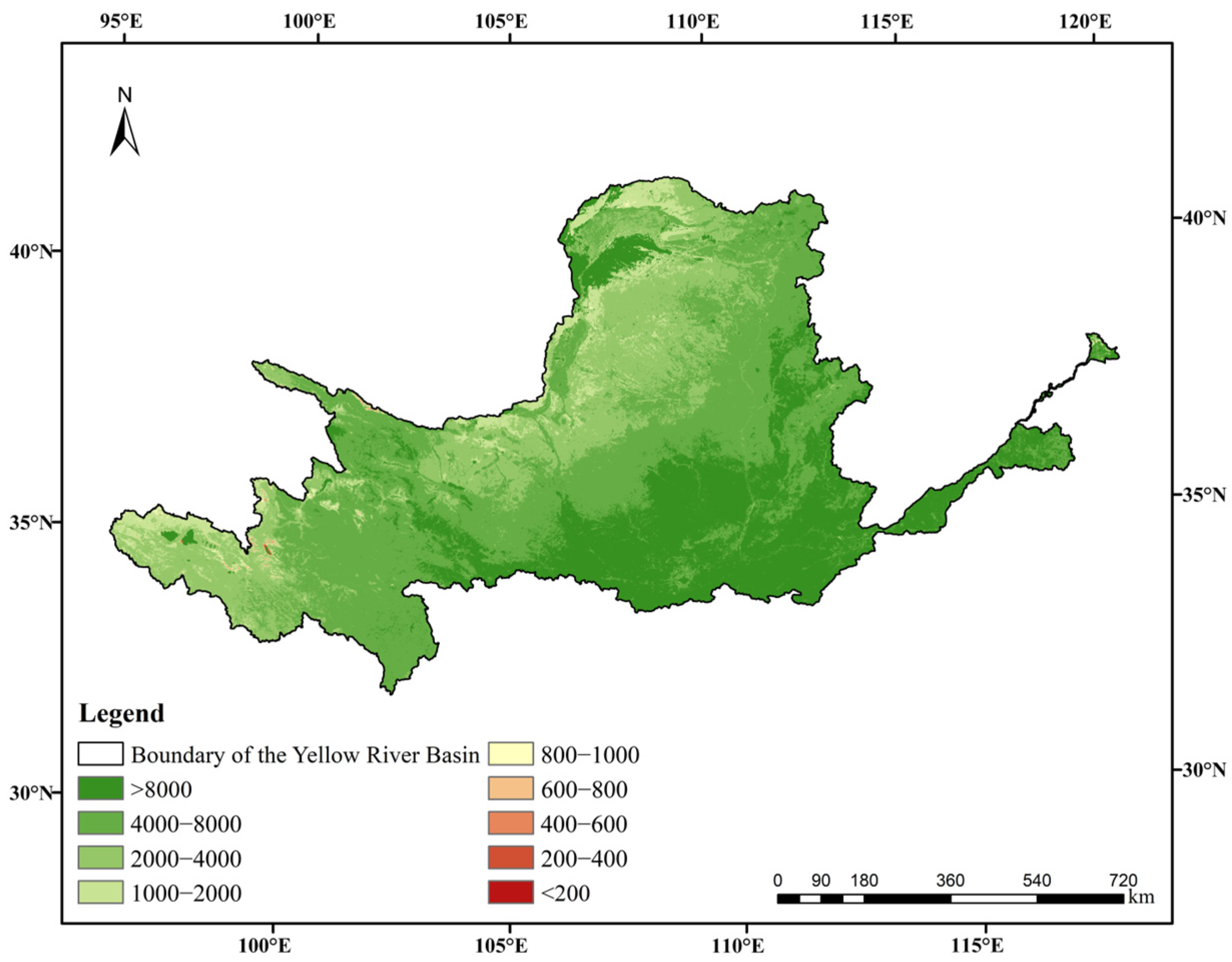
Through format conversion and projection transformation of the raw data, the corresponding wavebands were extracted to obtain time-series GPP products at a 500 m resolution (unit: g C/m²/year). Per previous reports [46,47], the GPP data were classified into nine levels, with those under 1000 divided by an interval of 200, and those above 1000 divided by 2000, 4000, and 8000 as the thresholds. Figure 3 shows the nine levels of GPP in YRB in 2024.

The fractional vegetation cover (FVC) was calculated based on MODIS-NDVI data. Specifically, with the dimidiate pixel model and NDVI data, the inversion model was employed to calculate FVC [48], as shown in Equation (1) [44]:

$$FVC={\displaystyle \frac{\left({NDVI}_i-{NDVI}_{min}\right)}{\left({NDVI}_{max}-{NDVI}_{min}\right)}}$$

(1)

where $FVC$ is the fractional vegetation cover, ${NDVI}_i$ is the NDVI value of a given pixel at a given time; ${NDVI}_{min}$ and ${NDVI}_{max}$ represent the minimum and maximum NDVI values obtained at a 5–95% confidence interval [49].

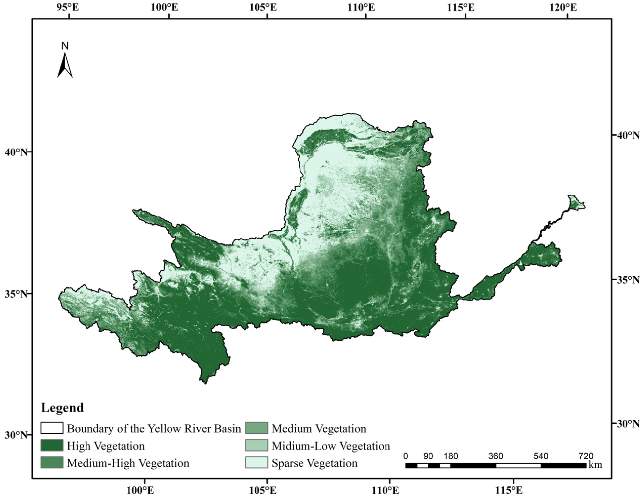
According to the existing standards for FVC classification [50] and the vegetation cover characteristics of YRB, five levels of vegetation cover were defined: low vegetation cover ($\mathrm{F}\mathrm{V}\mathrm{C}\le 0.3$), medium-low vegetation cover ($0.3<\mathrm{F}\mathrm{V}\mathrm{C}\le 0.45$), medium vegetation cover ($0.45<\mathrm{F}\mathrm{V}\mathrm{C}\le 0.6$), medium-high vegetation cover ($0.6<\mathrm{F}\mathrm{V}\mathrm{C}\le 0.75$), and high vegetation cover ($\mathrm{F}\mathrm{V}\mathrm{C}>0.75$). Figure 4 shows the distribution of vegetation cover levels in YRB in 2024.

The MOD17A3HGF GPP and the FVC derived from MODIS-NDVI products were validated against eddy covariance tower measurements globally, which were estimated to have an uncertainty of 10% based on validation studies [47,48,49,50].

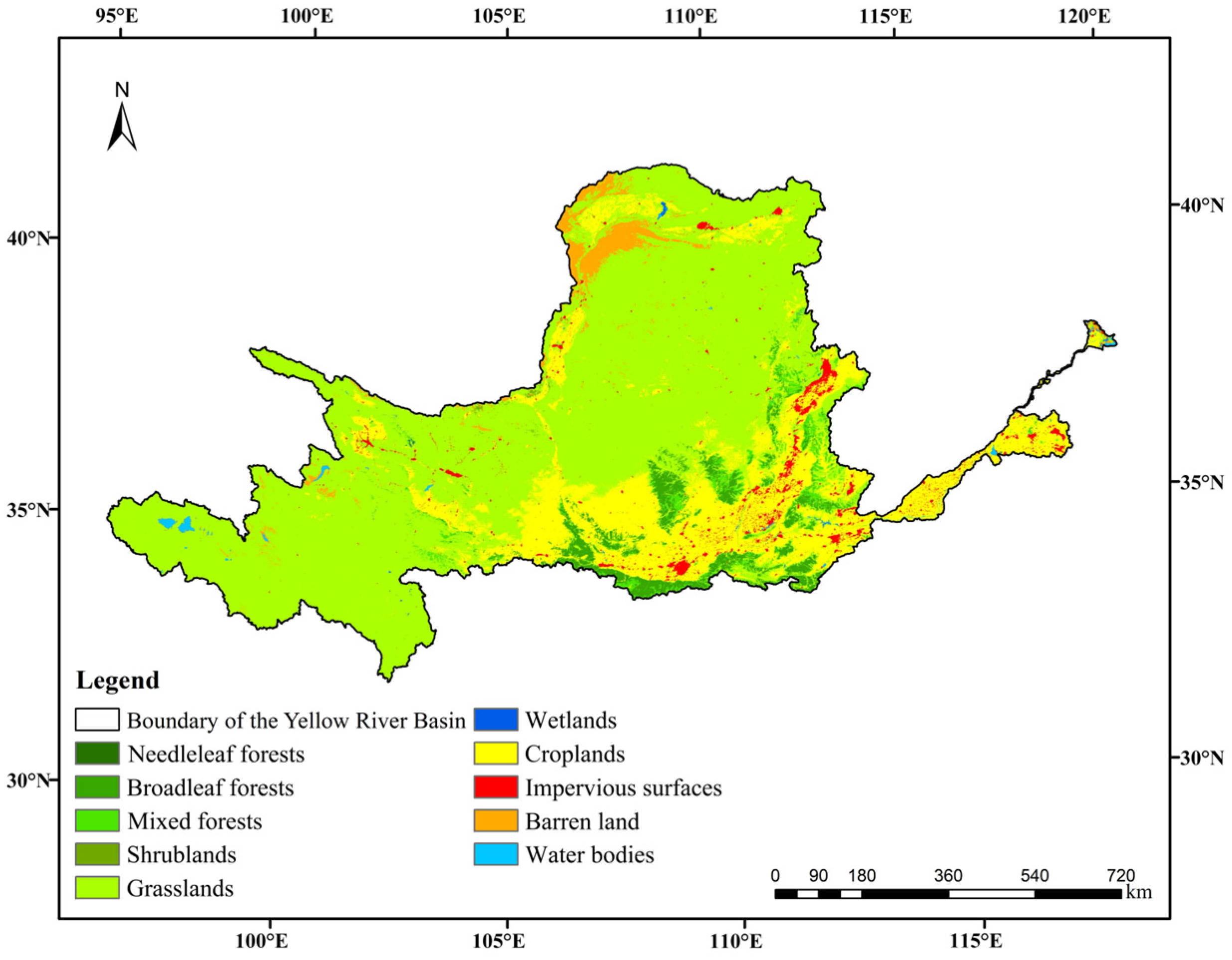
The LUCC data were classified per the International Geosphere-Biosphere Programme (IGBP), which identifies 17 LUCC types, including 11 natural vegetation types, 3 developed and mosaicked land types, and 3 non-vegetated land types [51]. For the sake of convenience in subsequent data processing, some land cover types were merged in the present work. The final LUCC classification results are presented in

Table 2. LUCC classification in this study.

Classification Code	LUCC Type	Classification Code	LUCC Type
1	Needleleaf forests	6	Wetlands
2	Broadleaf forests	7	Croplands
3	Mixed forests	8	Impervious surfaces
4	Shrublands	9	Barren lands
5	Grasslands	10	Water bodies

and Figure 5.

3.1.2. Spatial Overlay Analysis

Differences in the projection methods and geo-coordinates will introduce errors in data alignment and compromise the analysis accuracy [52]. Therefore, to ensure spatial alignment of all multi-source datasets and guarantee the accuracy of subsequent analyses, a rigorous spatial overlay preprocessing procedure was implemented here. All raster and vector data layers (including MODIS products, ASTER DEM, soil, and climate data) were unified into a shared geographic coordinate system and projection scheme. Specifically, all data were projected into the WGS 84/UTM Zone 49N (EPSG:32649) coordinate system. This projection was selected because it minimizes distortion across the vast east–west extent of the YRB.

This process was executed using the Project Raster and Project tools in ArcGIS Pro 3.0. During projection, the continuous remote-sensing data (e.g., GPP, FVC, climate raster) were resampled using the bilinear interpolation algorithm to preserve the spectral and continuous characteristics of the data, while categorical data (e.g., LUCC) were resampled using the nearest neighbor method to prevent the generation of invalid class values. The final resolution for all raster analysis was set to 500 m to fit the coarsest resolution of the MODIS products. The alignment accuracy was verified by controlling the root mean square error (RMSE) below 0.5 pixels during the georeferencing process.

3.1.3. Data Normalization

The objective of data normalization is to remove the influence of different data scales and enable data comparability [53]. The min–max normalization technique was employed in our work to convert data into values within the range of [0, 1], thereby making the data comparable under the same scale and improving the reliability of analysis results. It should be noted that the collected data of GPP and LUCC were at the annual scale, and their spatial variations were characterized by the spatial distribution and changes in the area of land of each category each year. As the MODIS-NDVI data were 16-day composite products, arithmetic averaging was performed to obtain interannual FVC data. Likewise, arithmetic averaging was also adopted to convert the monthly scale raster climate data into annual-scale climate outputs, and their spatial distribution was characterized by the changes in the grid pixel value, which partly reflected the hydrological dynamics at the stations. Elevation and soil data, which did not change significantly over time, were considered static in this study [49].

$$X={\displaystyle \frac{\left(X_i-X_{min}\right)}{\left(X_{max}-X_{min}\right)}}$$

(2)

where $X$ is the normalized pixel value; $X_i$ is the original value of a pixel; $X_{min}$ and $X_{max}$ are the minimum and maximum values of all values in the original data, respectively.

3.2. Spatiotemporal Variations

Visualization of spatiotemporal changes in key ecological variables, such as GPP, FVC, and LUCC, will provide insights into the dynamics of ecosystems and unveil their correlations with human activities and natural factors [54].

Gross primary productivity (GPP) reflects the carbon sequestration capacity of an ecosystem [55], and fractional vegetation cover (FVC) reflects the health and land degradation of an ecosystem [56]. In our work, the dynamic spatiotemporal changes in GPP and FVC were visualized to display the evolution pattern of the ecosystem and identify the key drivers of changes.

Land use and cover change (LUCC) is a key contributing factor to ecological variations [57]. Comparing the LUCC data at different time points can quantify the encroachment of urban expansion on vegetation cover and the impacts of agricultural land on the ecosystem. In addition, the regional topography, which primarily determines the distribution of water content, temperature, and soil nutrients, can affect the vegetation growth and hydrological processes [58]. Based on climate data (such as temperature and precipitation), the variations in the ecological variables under different climate conditions can be examined.

3.3. Correlation Analysis

Examining the interactions between the hydrological indicators (precipitation, runoff, and sediment) and ecological variables will provide more insights into the correlations between the hydrological process and the ecological condition [59,60]. Precipitation is a key driver of runoff and sediment transport [25,26]; their linear and nonlinear correlations can be revealed by Pearson correlation analysis and Spearman correlation analysis, respectively [61]. Meanwhile, GPP and FVC are closely correlated to hydrological factors, including precipitation, runoff, and sediment [62]. Correlation analysis can quantify the correlations between these ecological variables and the hydrological factors [59]:

$$r={\displaystyle \frac{\sum _{i=1}^n\left(X_i-\overline{X}\right)\left(Y_i-\overline{Y}\right)}{\sqrt{\sum _{i=1}^n{\left(X_i-\overline{X}\right)}^2}\sqrt{\sum _{i=1}^n{\left(Y_i-\overline{Y}\right)}^2}}}$$

(3)

where $r$ is the correlation coefficient between variables $x$ and $y$; $n$ is the sample size; $X_i$ and $Y_i$ are the values of the sample in the $i$-th unit; $\overline{X}$ and $\overline{Y}$ are the sample means of variables $x$ and $y$.

Moreover, as the response of ecological variables to the hydrological factors may show a lag effect [40], cross-correlation analysis was performed here to measure this time lag effect and thereby deepen the understanding of the dynamic correlations between hydrological factors and the ecosystem.

3.4. Driving Mechanism

Hydrological factors (precipitation, runoff, and sediment, etc.), climate factors, and land use types have significant impacts on the GPP and FVC of an ecosystem. Data-driven models can be employed to identify the key drivers of ecological variations and quantify the impacts of each driver. Here, the random forest (RF) model and the geographical detector (GD) model were employed to identify the key drivers of variations in GPP and FVC.

• Random forest (RF) model

The RF model can handle high-dimensional nonlinear data and assess the importance of variables, characterized by advantages including bootstrap sampling, assembly prediction, high accuracy, and strong robustness [63]. This model improves prediction robustness by integrating multiple decision trees, and its core mechanism includes triple randomness:

Data random sampling: Bootstrap sampling was used to generate k training subsets {D₁, …, D_k} from the original dataset D.

Feature random selection: In the construction of a single tree, $m_{try}$ candidate features (usually $m_{try}=\sqrt{m}$) are randomly selected from all $m$ features to generate split nodes [62].

$$\widehat{j}={argmin}_{j\in M_{try}}\sum _{i\in node}{\left(y_i-{\overline{y}}_L\right)}^2+{\left(y_i-{\overline{y}}_R\right)}^2$$

(4)

Among them, ${\overline{y}}_L$ and ${\overline{y}}_R$ are the means of the left and right child node samples, respectively; and $M_{try}$ is the random feature subset.

Decision tree ensemble: The final prediction result is the mean (regression task) or mode (classification task) output by k trees [62].

$${\widehat{y}}_{RF}={\displaystyle \frac{1}{k}}\sum _{t=1}^k{T}_t\left(X\right)$$

(5)

In this study, with GPP and FVC as the dependent variables, and the climate, topography, soil, and LUCC as independent variables, an RF model was built; meanwhile, the variable importance score (VIS) was introduced to measure the contribution of each factor to GPP and FVC. The data were divided into a training set and a test set by a ratio of 7:3 [41], and the VIS of each independent variable was calculated to measure their respective contribution to and impacts on the variations in the dependent variables (GPP or FVC).

2.

Geographical detector (GD) model

The GD model is often used to identify spatial heterogeneity of geographical phenomena and their driving factors. This model calculates the explanatory power of each driving factor for a geographic phenomenon (represented by a q value within the range [0, 1]) and measures their impacts on the spatial distribution pattern of the phenomenon in question [41]. The model used in this study follows the classic paradigm of geographic detectors and adopts equidistant classification for continuous variables, which has broad comparability [42]. The number of categories was uniformly set to 5, basically conforming to the optimal range of the geographic detector [43]. In this study, the GD model was employed to calculate the impacts of the driving factors on the spatial distribution of the ecological variables and detect their interactions. The q value calculation is shown in Equation (6) [64]:

$$q=1-{\displaystyle \frac{\sum _{h-1}^L{N}_h{\sigma }_h^2}{N{\sigma }^2}}$$

(6)

where $N_h$ indicates the number of samples in the sub-area $h$; ${\sigma }_h^2$ is the variance of the sub-area $h$; $N$ is the sum of samples; ${\sigma }^2$ is the total variance.

The discretization of continuous driving factors exerts significant impacts on the p-value calculation and hence accounts for a critical step in the GD model. To ensure the robustness and optimality of our results, we employed the optimal parameter-based geographical detector (OPGD) approach to determine the most appropriate discretization method and number of categories for each factor [44]. This method iteratively tests different classification algorithms (including natural breaks, quantiles, and equal intervals) and a range of category numbers to find the parameter set that maximizes the q-value for each factor, thereby achieving the highest explanatory power. Ultimately, the quantile method with five categories was identified as the optimal discretization strategy for most continuous variables in this study, which is consistent with the recommended practice in geographical detector applications.

4. Results

4.1. Variation in Ecological Environment

4.1.1. Dynamic Changes in GPP and FVC

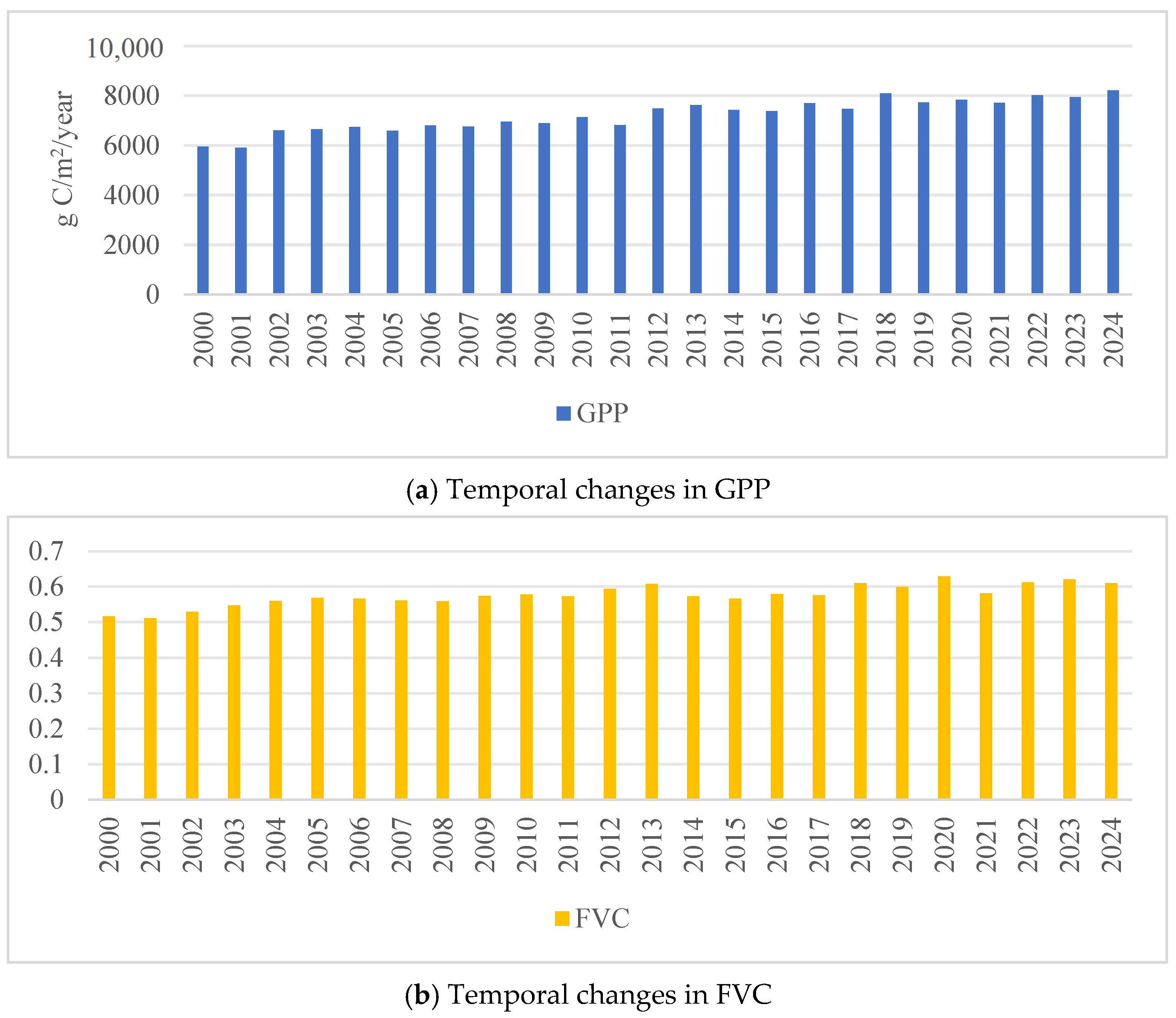
The annual changes in the GPP and FVC in YRB in 2000–2024 were measured, as shown in Figure 6.

As Figure 6 shows, over the 25 years, both GPP and FVC showed an upward trend in YRB, indicating substantially improved vegetation growth and vegetation cover. Specifically, from 2000 to 2024, GPP grew by 37.9% from 5960.72 g C/m²/year to 8219.01 g C/m²/year, and FVC increased by 18.0% from 0.52 to 0.61. Despite the overall upward trend, small fluctuations were observed: GPP witnessed a decline in the years 2005, 2011, 2014, and 2015; and FVC exhibited a slight decrease in 2011, 2014, and 2015.

The temporal changes in GPP and FVC levels in YRB from 2000 to 2024 were investigated and visualized, as shown in Figure 7.

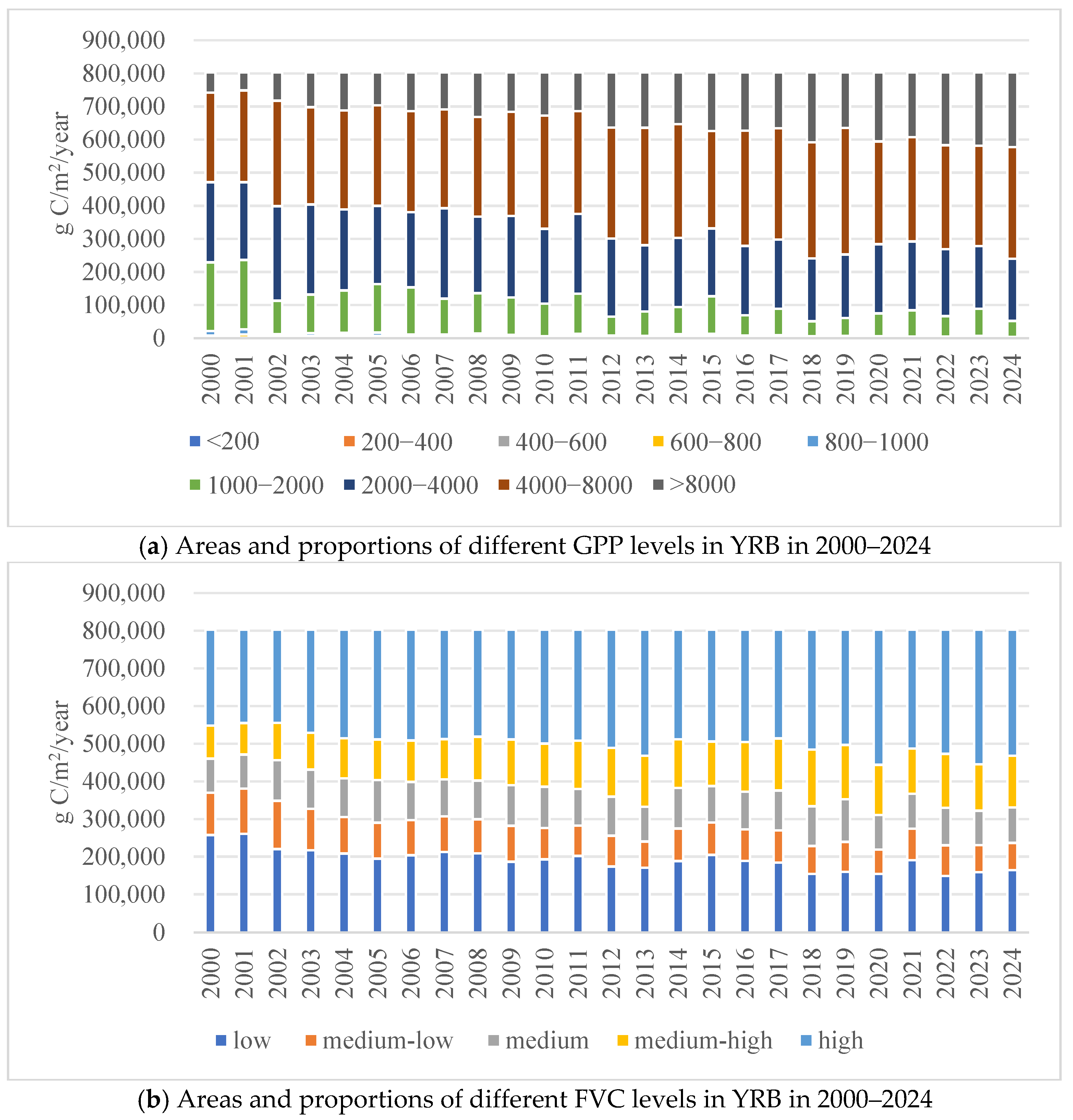
As Figure 7a shows, the area and proportion of GPP levels changed over the 25 years of study: in 2000, the area of regions with a 1000–2000 GPP was 207,142.50 km², which declined to 48,774.25 km² in 2024, exhibiting a sharp decline. Likewise, the area of regions with a 2000–4000 GPP declined (from 242,326.25 km² to 187,787.75 km²), suggesting a decline in the area of regions with a medium-high productivity level across the basin over the 25 years. However, the area of regions with a 4000–8000 GPP rose from 270,766.75 km² to 337,880.25 km², indicating an increased area of regions with a high level of productivity. As Figure 7b shows, over the 25 years, the area with low and medium-low levels of vegetation cover declined from 257,354 km² to 164,351.75 km² and from 112,387.5 km² to 72,401.5 km², respectively, indicating improved vegetation cover across the years; moreover, all the areas with medium, medium-high, and high levels of vegetation cover increased, implying a growing area of high vegetation cover in the basin.

The spatial distribution of GPP and FVC levels across the 25 years in YRB was investigated by extracting the mean values, and the result is presented in Figure 8.

As Figure 8a shows, the GPP increased from west to east; regions with a lower GPP included the origin of the Yellow River, the upper reaches, and some parts of the middle reaches of the YRB, whereas a higher GPP was observed in the middle and lower reaches of the basin, excluding the Loess Plateau. As Figure 8b shows, FVC shared a similar pattern of spatial distribution as GPP, but with a few exceptions: a higher FVC was observed in the mid-upper reaches of the basin and the Loess Plateau, while a lower FVC was found in the estuary delta of the Yellow River. The significant increase in GPP (37.9%) and FVC (18.0%) aligned with regional studies that reported vegetation recovery in YRB since 2000: Wang et al. [8] documented a 34% GPP rise in the Loess Plateau, and Lin et al. [10] observed a 15–20% FVC growth in semi-arid zones. The alignment with previous reports confirmed basin-wide greening trends driven by ecological restoration policies.

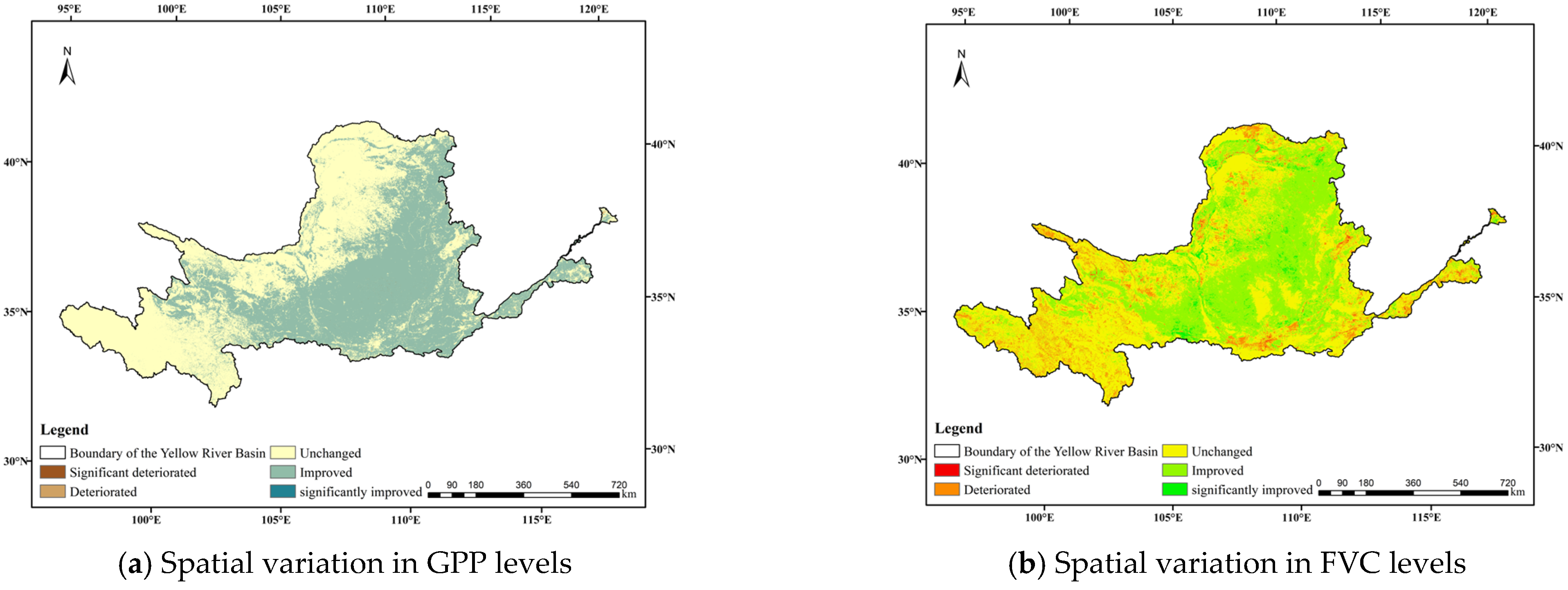
By comparing the changes in GPP and FVC values between 2024 and 2000, the spatial variation trends of ecological parameters in the YRB can be obtained, as shown in Figure 9.

As Figure 9a shows, the GPP in the middle and lower reaches of YRB was improving, while in the GPP changes in the middle and upper reaches were not significant, and a small part of the estuary area showed significant deterioration. Figure 9b indicates that FVC in the Yellow River source area, the surrounding areas of the Loess Plateau, and the downstream plain area partially deteriorated, while the FVC in the upper and middle reaches of the Yellow River and the central area of the Loess Plateau exhibited obvious improvement. Overall, the hotspots of ecological improvement were mainly observed in the Loess Plateau region, which is largely attributed to gully cultivation and greening projects. In contrast, occasional ecological degradation was observed in the urban outskirts of major cities such as Lanzhou and Zhengzhou, which may be related to urban expansion.

4.1.2. Spatiotemporal Variations in LUCC

The LUCC data in YRB from 2000 to 2024 were overlaid with the GPP and FVC data of corresponding time periods to generate a land use transition matrix.

Table 3. Land use transition matrix in YRB in 2000–2024.

		2024										Total (2000)
		Needleleaf Forests	Broadleaf Forests	Mixed Forests	Shrublands	Grasslands	Wetlands	Croplands	Impervious Surfaces	Barren Lands	Water Bodies
2000	Needleleaf forests	34.25	0	47.75	0	2.75	0.25	0	0	0	0	85
	Broadleaf forests	0	16,340.75	903	6.25	781.25	0	11.75	0	0	0	18,043
	Mixed forests	5.75	2488.25	4239.25	0.5	82.25	5.25	0	0	0	0	6821.25
	Shrublands	0	65	9.75	164.5	25,847.25	0	132.25	1.25	63.25	0	26,283.25
	Grassland	55.5	9021.25	7596.25	501.5	485,547.5	526	68,864.25	432.75	2006	86.25	574,637.25
	Wetland	21.75	126	449.25	1	323.5	263.5	10.5	1.75	22.5	49.75	1269.5
	Croplands	0.25	3253.75	63	42	11,303.5	149.75	98,752	633	91.5	11.25	114,300
	Impervious surfaces	0	0	0	0	0	0	0	14,725.25	0	0	14,725.25
	Barren lands	0	0	0	152.25	23,966.25	111	101	20.75	19,440	245.25	44,036.5
	Water bodies	0	0	0	0	2.75	11.25	0	1.5	32.75	2309	2357.25
Total (2024)		117.5	31,295	13,308.25	868	547,857	1067	167,871.75	15,816.25	21,656	2701.5	−
Dynamic changes		32.5	13,252	6487	−25,415.25	−26,780.25	−202.5	53,571.75	1091	−22,380.5	344.25	−

shows the land use transition matrix.

As shown in Table 3, overall, the land use types that showed the most significant transitions included grasslands, croplands, and impervious surfaces. Specifically, the area of grasslands dropped by 26,780.25 km² from 574,637.25 km² in 2000 to 547,857 km² in 2024; the area of croplands rose by 53,571.75 km² from 114,300 km² in 2000 to 167,871.75 km² in 2024, indicating pronounced expansion of croplands over the 25 years; the area of impervious surfaces grew by 1091 km² from 14,725.25 km² to 15,816.25 km², indicating accelerated urbanization in the 25 years. Other land use types also showed variations: the area of needleleaf forests grew from 85 km² to 117.5 km², that of broadleaf forests rose from 18,043 km² to 31,295 km², and the area of mixed forests increased from 6821.25 km² to 13,308.25 km²; in contrast, the area of shrublands shrank from 26,283.25 km² to 868 km², and that of barren land declined sharply from 44,036.5 km² to 21,656 km²; the area of other land use types exhibited little changes. In sum, significant variations were found in the land use types in YRB over the 25 years, dominated by the expansion of croplands and impervious surfaces, as well as declines in the area of grasslands, shrublands, and barren lands. These changes reflected the impact of human activities, especially agricultural expansion and accelerated urbanization, on the natural environment; meanwhile, the increased area of needleleaf forests, broadleaf forests, and mixed forests implied the positive feedback to eco-restoration and eco-protection measures adopted in the basin over these years.

To further elucidate how the specific land use transition processes contributed to the overall changes in ecological indicators, we linked the transition matrix with the characteristic GPP and FVC values of each land use type.

Analysis of the net changes reveals a dominant pattern: the extensive conversion of grasslands to croplands. On average, croplands exhibited a slightly higher GPP (11,328.98 g C/m²/year) compared to grasslands (10,236.52 g C/m²/year) during the study period. Similarly, the mean FVC of croplands (0.97) was also higher than that of grasslands (0.91). Therefore, the net increase of 53,571.75 km² in cropland area—much of which was converted from grasslands—directly contributed to the basin-wide increase in GPP and FVC. This transformation represents a quintessential example of human activities (agricultural expansion) driving ecological changes by replacing a natural vegetation type with a more productive but potentially less resilient managed ecosystem.

Conversely, the expansion of impervious surfaces (by 1091 km²), which typically have near-zero GPP and FVC, exerted a localized negative pressure on the ecological environment, although its basin-wide influence was outweighed by the positive contribution from agricultural expansion.

This linkage between the macro-level driver (LUCC) and the predominant micro-level process (grassland-to-cropland conversion) robustly explains the mechanisms behind the observed ecological improvements, highlighting the profound impact of anthropogenic land management on the basin’s carbon and water cycles.

4.1.3. Coupling Between Ecological Variables and Climate Factors

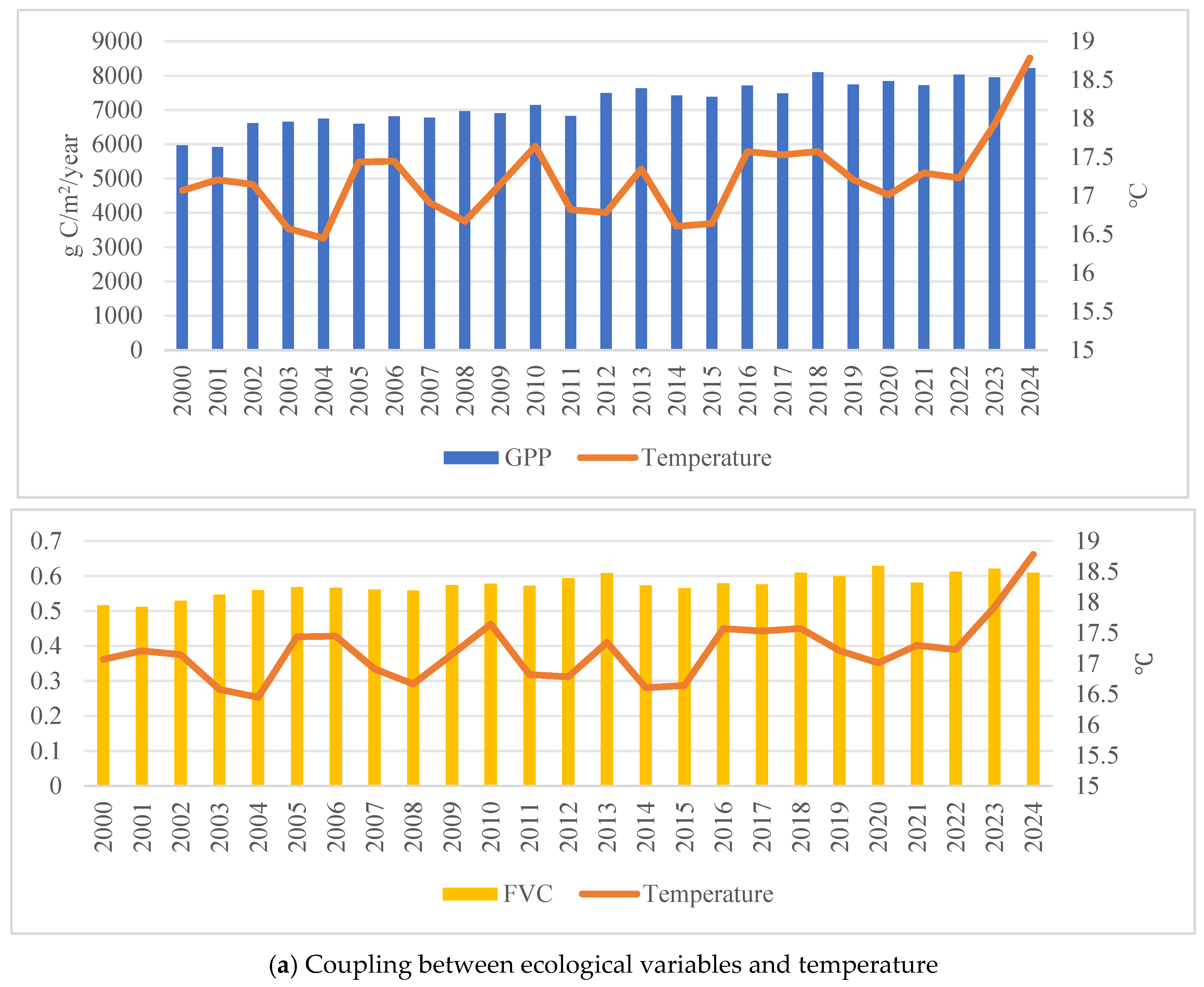
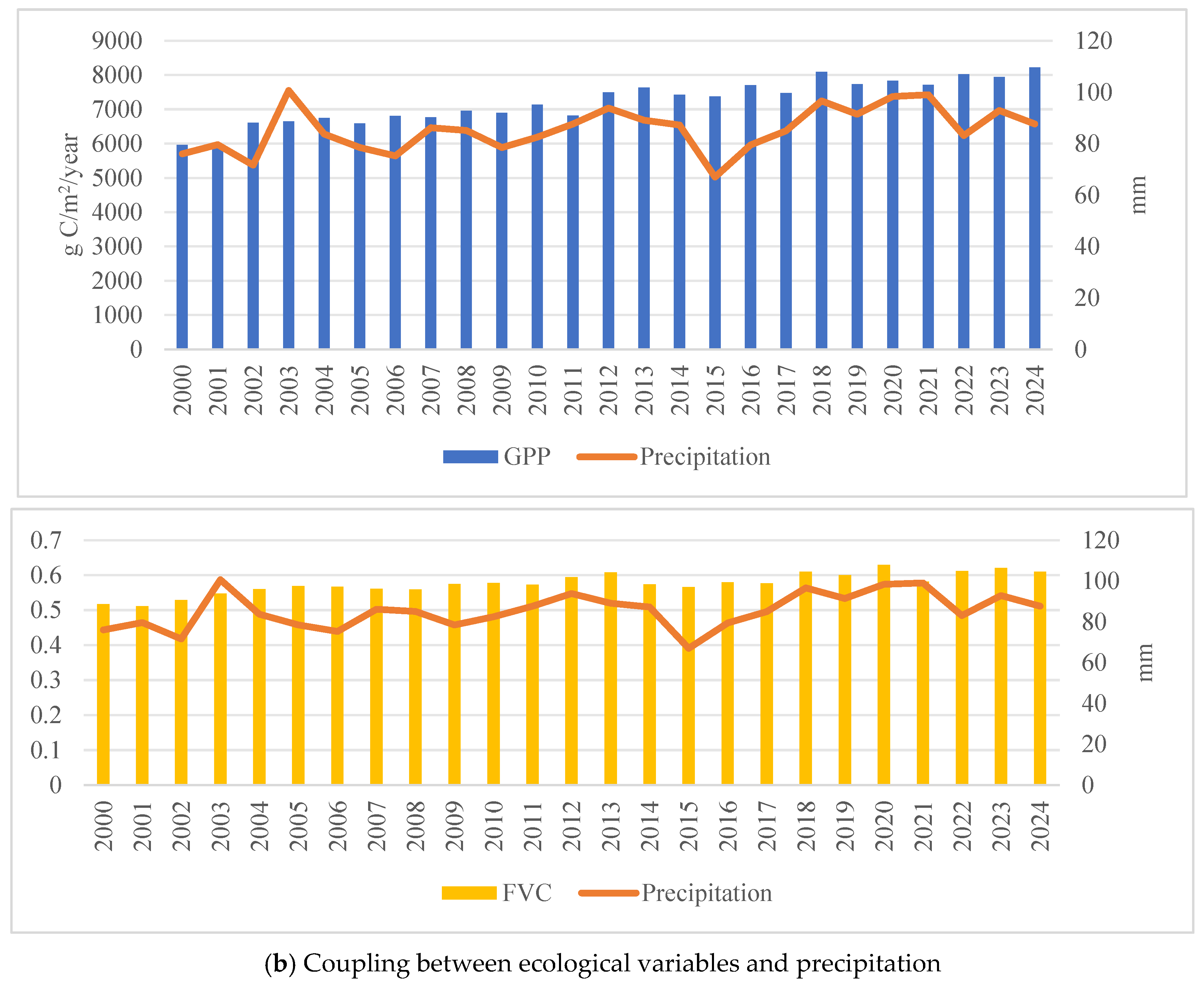
The coupling relations between the dependent variables (GPP and FVC) and the climate factors (temperature and precipitation) were examined, as shown in Figure 10.

As Figure 10 shows, the GPP and FVC exhibited a complex coupling relation with the temperature and precipitation in YRB in 2000–2025. The temperature exerted a significant impact on both GPP and FVC: in normal cases, years with a high temperature (such as 2000, 2010, 2016, 2018, 2021, and 2023) showed a high GPP and FVC, indicating that an increase in the temperature promoted vegetation growth and improved vegetation cover in the basin. However, GPP and FVC remained high in some years with a lower temperature (such as 2003, 2007, 2022, and 2024), implying that the temperature was not the sole contributing factor to variations in GPP and FVC. Precipitation also had a significant impact on GPP and FVC: years with more rainfall (such as 2000, 2003, 2012, 2018, 2021, and 2024) had higher GPP and FVC, suggesting that increased rainfall contributed positively to vegetation growth and cover. However, GPP and FVC remained high in some years with less precipitation (such as 2015 and 2023), suggesting that precipitation was not the sole influencing factor either. In sum, the temperature and precipitation had a complex coupling relationship with GPP and FVC, both exerting an impact on vegetation growth and cover.

4.2. Hydrological Processes

4.2.1. Evolution Pattern and Spatial Distribution of Hydrological Processes

In this study, runoff and sediment data were obtained from hydrological stations in YRB from 2000 to 2023. Supplementary Table S1 shows the collected data from the upper reaches to the lower reaches of YRB, and missing data are represented by “–”.

Significant spatiotemporal heterogeneity was observed in the evolution pattern and spatial distribution of hydrological variables. Temporally, the annual runoff and sediment transport showed substantial changes from 2000 to 2023. As measured at Tangnaihai Station in the upper reaches of the YRB, the runoff reached the peak (32.16 billion m³) and the bottom (10.58 billion m³) in 2020 and 2002, respectively; the largest sediment transport (21.1 million t) and smallest sediment transport (2.8 million t) were observed in 2018 and 2008, respectively. In Lanzhou Station, the annual runoff exhibited an upward trend across the years, growing from 23.56 billion m³ in 2001 to 50.45 billion m³ in 2020; the highest annual sediment transport (96 million t) and the lowest annual sediment transport (5.8 million t) occurred in 2018 and 2021, respectively. At Toudaoguai Station in the middle reaches of the YRB, the highest annual runoff (36.98 billion m³) and the lowest annual runoff (11.31 billion m³) were observed in 2020 and 2016, respectively; the maximum and minimum sediment transport (144 million t and 16.3 million t) were observed in 2019 and 2016. In Longmen Station, the annual runoff reached the maximum (38 million m³) and the minimum (13.94 million m³) in 2019 and 2001, respectively; the annual sediment transport reached the maximum (335.2 million t) and the minimum (37.8 million t) in 2002 and 2014, respectively. At stations in the lower reaches of Yellow River, including Tongguan Station, Huayuankou Station, Gaocun Station, Aishan Station, and Lijin Station, the annual runoff demonstrated similar patterns of changes; the annual runoff at Huayuankou Station and Lijin Station reached 50.97 billion m³ and 44.11 billion m³, respectively, in 2020, and the annual sediment transport at Tongguan Station and Huayuankou Station reached 617.9 million t and 344 million t in 2003 and 2018, respectively, indicating a significant increase in the annual runoff and sediment transport in the lower reaches of YRB.

Spatially, the annual runoff and annual sediment transport showed an upward trend from the upper to the lower reaches of YRB. Stations in the upper reaches, such as Tangnaihai and Lanzhou Stations, had a low annual runoff and sediment transport; the values in the middle reaches, as measured in Toudaoguai and Longmen stations, were relatively higher than the measurements in the upper reaches; and the values in the lower reaches of YRB, as measured in Tongguan, Huayuankou, and Lijin, were significantly higher. This distribution pattern was closely correlated to the topography, precipitation distribution, and human activities in the basin: the upper reaches had a higher altitude, less precipitation, and stronger evaporation; in the middle reaches, increased precipitation and water influx from tributaries led to a higher annual runoff and sediment transport. The lower reaches, due to a further increase in precipitation and influx from tributaries, exhibited a significantly higher annual runoff and sediment transport.

4.2.2. Changes in Runoff Generation and Sediment Transport Capacity of Precipitation

The changes in rainfall runoff and sediment transport capacity in the Yellow River Basin are closely related to precipitation, terrain, vegetation coverage, and human activities. The precipitation in YRB showed a spatial trend of gradually increasing from upstream to downstream. The annual precipitation at the upstream Tangnaihai station fluctuated greatly between 2000 and 2023, with the highest value occurring in 2018 (103.825 mm) and the lowest value occurring in 2022 (49.8 mm). The annual precipitation at Lanzhou Station fluctuated greatly between 2000 and 2023, with the highest value occurring in 2022 (103.0 mm) and the lowest value occurring in 2021 (43.2 mm). The annual precipitation of Toudaoguai Station and Longmen Station in the middle reaches also showed significant fluctuations. The annual precipitation of Toudaoguai Station reached its peak in 2012 (107.475 mm) and the lowest value appeared in 2005 (53.8 mm), while that of Longmen Station reached its peak in 2003 (146.575 mm) and the lowest value appeared in 2001 (72.8 mm). The annual precipitation of Tongguan Station, Huayuankou Station, Gaocun Station, Aishan Station, and Lijin Station downstream also showed similar fluctuations, with almost all the highest values occurring in 2021 (Huayuankou Station 254.92 mm, Aishan Station 197.867 mm, Lijin Station 144.95 mm), which then tended to flatten out. The precipitation of downstream stations showed a significant increase compared to the middle and upper reaches. The data are shown in Supplementary Table S2.

The rainfall runoff capacity of YRB is closely related to precipitation, terrain, and vegetation coverage. The rainfall runoff capacity of Tangnaihai Station and Lanzhou Station in the upper reaches of the basin was relatively low, which is related to the lower precipitation, greater evaporation, and lower vegetation coverage there. The rainfall runoff capacity of Toudaoguai Station and Longmen Station in the middle reaches increased, which is related to the increased precipitation in the middle reaches and the influence of terrain. The rainfall runoff capacity of downstream Tongguan Station, Huayuankou Station, and Lijin Station significantly increased, which is related to the further increase in precipitation in downstream areas and the convergence effect of the Yellow River main stream.

4.2.3. Response of Ecological Indicators to Hydrological Factors

Supplementary Table S3 shows the variations in the ecological indicators from 2000 to 2023 in YRB. Significant variations were observed in the ecological indicators in YRB over those years. In the upper reaches of the basin, Tangnaihai Station witnessed the highest GPP (3010 g C/m²/year) in 2004 and the lowest GPP (1673 g C/m²/year) in 2013; the FVC there reached the maximum (0.482) in 2004 and the minimum (0.052) in 2022. At Lanzhou Station, the FVC reached the maximum (0.208) in 2001 and the minimum (0.000) in 2002. In the middle reaches of the basin, Toudaoguai Station reached the maximum GPP (5112 g C/m²/year) in 2019 and the minimum GPP (1862 g C/m²/year) in 2001; and the FVC there reached the peak (0.702) in 2016 and the minimum (0.304) in 2001. At Longmen Station, the maximum GPP occurred in 2023 (6045 g C/m²/year) and the minimum GPP was observed in 2011 (2218 g C/m²/year); the FVC there reached the peak in 2004 (0.797) and the bottom in 2012 (0.073). Stations in the lower reaches of the basin generally exhibited a higher GPP and FVC than stations in the upper and middle reaches. In particular, the GPP in Tongguan Station and Huayuankou Station reached 9303 g C/m²/year and 5405 g C/m²/year in 2022 and 2001, respectively, and the FVC value at these two stations reached 0.808 and 0.877 in 2010 and 2001, respectively.

Significant responses of ecological indicators (GPP and FVC) to hydrological processes (annual runoff and annual sediment transport) were observed in YRB from 2000 to 2023. Specifically, years with a higher annual runoff exhibited a higher GPP and FVC, indicating a significant correlation between the ecological indicators and the hydrological processes; years with a larger sediment transport showed a lower GPP and FVC, suggesting negative impacts of sediment transport on GPP and FVC.

Pearson correlation and Spearman correlation analyses were performed to reveal the correlations between precipitation, runoff, sediment, and the ecological indicators, as shown in

Table 4. Pearson correlation analysis results.

Hydrological Station	Precipitation vs. GPP	Precipitation vs. FVC	Runoff vs. GPP	Runoff vs. FVC	Sediment vs. GPP	Sediment vs. FVC
Tangnaihai	0.72	0.68	0.75	0.70	−0.55	−0.60
Lanzhou	0.65	0.62	0.70	0.68	−0.50	−0.55
Toudaoguai	0.78	0.74	0.80	0.76	−0.60	−0.65
Longmen	0.82	0.80	0.85	0.82	−0.70	−0.75
Tongguan	0.85	0.83	0.88	0.85	−0.75	−0.80
Huayuankou	0.80	0.78	0.83	0.80	−0.65	−0.70
Lijin	0.78	0.75	0.82	0.78	−0.60	−0.65

and

Table 5. Spearman correlation analysis results.

Hydrological Station	Precipitation vs. GPP	Precipitation vs. FVC	Runoff vs. GPP	Runoff vs. FVC	Sediment vs. GPP	Sediment vs. FVC
Tangnaihai	0.75	0.70	0.78	0.72	−0.58	−0.62
Lanzhou	0.68	0.65	0.72	0.70	−0.52	−0.57
Toudaoguai	0.80	0.76	0.82	0.78	−0.62	−0.68
Longmen	0.85	0.82	0.88	0.85	−0.72	−0.78
Tongguan	0.88	0.85	0.90	0.88	−0.78	−0.82
Huayuankou	0.82	0.80	0.85	0.82	−0.68	−0.72
Lijin	0.80	0.78	0.84	0.80	−0.62	−0.68

.

As Table 4 and Table 5 show, a strong positive correlation was observed between precipitation and the ecological indicators (GPP and FVC), and this correlation was the strongest in the middle and lower reaches of YRB (as evidenced by data for Tongguan, Huayuankou, and Lijin Stations), which implies that increased precipitation improved vegetation growth and cover. The runoff also exhibited a positive correlation to the ecological indicators, and the most significant correlation was found in the lower reaches of the basin (Huayuankou and Lijin Stations), which means increased runoff provided more water resources for vegetation growth. However, the sediment was found to be negatively correlated to the ecological indicators, and this negative correlation was most pronounced at Longmen and Tongguan Stations, which suggests that increased sediments inhibited vegetation growth and cover.

In addition, cross-correlation analysis was performed to unveil the time-lag effect in the response of ecological indicators to precipitation, runoff, and sediment. The results are shown in

Table 6. Cross-correlation analysis results.

Stations	Precipitation vs. GPP	Runoff vs. FVC	Sediment vs. GPP
	One-Year Lag Correlation Coefficient	Two-Year Lag Correlation Coefficient	One-Year Lag Correlation Coefficient
Tangnaihai	0.70	0.72	−0.60
Lanzhou	0.65	0.68	−0.55
Toudaoguai	0.75	0.78	−0.65
Longmen	0.80	0.82	−0.70
Tongguan	0.85	0.88	−0.75
Huayuankou	0.78	0.80	−0.68
Lijin	0.75	0.78	−0.65

.

As Table 6 shows, the impact of precipitation on the ecological indicators reached the peak 1–2 years later, indicating the presence of time lags in the impact of precipitation on vegetation growth; a similar time-lag effect was observed in the impact of the runoff on GPP and FVC, and this was most prominent in the lower reaches of the basin, where an increase in the runoff led to improved vegetation productivity 1–2 years later. The negative impact of sediment transport on GPP and FVC also exhibited a time-lag effect, where the inhibitory effect of the sediment transport on vegetation growth and productivity took place 1–2 years later.

Overall, in 2000–2023, the precipitation and runoff positively affected the vegetation growth in YRB, whereas the sediment transport exerted a negative impact. The impact of precipitation and runoff showed a time lag of 1–2 years, which means it took some time before the vegetation responded to variations in the hydrological processes; the negative impact of sediment transport on the ecological indicators also showed a time-lag effect, which means the damage of sediment accumulation on the ecological environment was incremental. The 1–2 year lagged negative response of GPP and FVC to sediment transport (Table 6) was consistent with the delayed vegetation damage mechanisms observed in high-erosion basins like the Yangtze River Basin (Lasanta et al. [40]), while the positive runoff–GPP correlation was aligned with findings in global meta-analyses of floodplain ecosystems (Bunn et al. [8]).

4.3. Coupling Analysis

4.3.1. Coupling Analysis Based on the RF Model

With GPP and FVC as the dependent variables, and climate, topography, soil, and land use indicators as the independent variables, a random forest (RF) model was constructed to unveil their coupling correlations, as shown in

Table 7. Importance of driving factors measured by the RF model.

GPP Model Variable Importance Score			FVC Model Variable Importance Score
7	LUCC	0.5072	7	LUCC	0.4019
6	DEM	0.1537	6	DEM	0.1719
5	Slope	0.1090	5	Slope	0.0954
4	Aspect	0.0971	4	Aspect	0.0929
3	Temp	0.0452	3	Precip	0.0762
2	PET	0.0345	2	Temp	0.0721
1	Soil	0.0288	1	PET	0.0638
0	Precip	0.0245	0	Soil	0.0261
GPP Model MSE		0.4415	FVC Model MSE		0.0133

.

As the GPP model variable importance score (VIS) in Table 7 shows, LUCC exhibited the strongest impact on GPP, with a VIS of 0.5072, significantly higher than the scores of other variables for GPP. The overwhelmingly stronger impact of LUCC on GPP suggests that changes in the land use types caused by human activities had the strongest and most far-reaching impact on the primary productivity of vegetation in YRB. The topographic indicators—DEM and slope—exhibited the second and third highest VIS for GPP, indicating that the topographical factors affected the spatial distribution pattern of GPP by changing lighting conditions, as well as the distribution of water and soil nutrients. In contrast, soil and climate factors, including temperature, potential evapotranspiration (PET), and precipitation, had a much lower VIS for GPP. However, the GPP model’s MSE was high (0.4415), and the reasons could be the following: First, GPP is a complex ecological process driven by a range of nonlinear interactions between various driving factors, and though the RF model can capture part of the nonlinear features, it is likely to overlook some key mechanisms. Second, unsatisfactory resolution and quality of the input data may undermine the model’s performance. Third, the lack of explicit modeling of physiological differences between vegetation types can also introduce modeling errors.

In the FVC model, LUCC was also identified as the most important driver (0.4019), but its VIS for FVC was slightly lower than its score for GPP, indicating that FVC was less sensitive to LUCC than GPP was. The climate factors reached a higher VIS for FVC than for GPP: the VIS of precipitation and temperature reached 0.0762 and 0.0721, respectively, which means FVC was more susceptible to the impact of water content and heat than GPP was. The VIS of DEM for FVC remained high (0.1719), suggesting that the regional topography indirectly shaped the vegetation cover pattern through its impact on the regional climate and soil conditions. Meanwhile, it is noteworthy to mention that PET had a higher VIS for FVC (0.0638) than for GPP (0.0345). This is because PET, a measure of the need for water in the atmosphere, directly affects the water stress of vegetation, and hence, FVC is more sensitive to PET than GPP is. The FVC model’s MSE was 0.0133, which was significantly lower than that of the GPP model (0.4415), providing an estimate of the model’s prediction uncertainty, and this difference is of methodological significance. FVC is a direct characterization of vegetation cover, and the accuracy of remote-sensing inversion of FVC (such as NDVI-based estimation) is usually high, and it shows a more direct and linear response to the driving factors. Moreover, the lower MSE of the FVC model also verified the reliability of the RF model in vegetation cover prediction. LUCC’s dominance as the primary driver of GPP variations (VIS = 0.5072 in RF, q = 0.4167 in GD) agrees with the findings by Gao et al. [54].

4.3.2. Identification of Drivers by the GD Model

With the normalized data of GPP and FVC, as well as the measured data of climate, topography, soil, and land use, a GD model was built, and the q value of each variable was calculated to analyze the coupling relations, as shown in

Table 8. Explanatory power of driving factors calculated by the GD model.

Factor	GPP			FVC
	Avg_Q	Min_Q	Max_Q	Avg_Q	Min_Q	Max_Q
DEM	0.0054	0.0040	0.0073	0.0584	0.0385	0.0948
Slope	0.0008	0.0005	0.0014	0.0115	0.0059	0.0151
Aspect	0.0003	0.0002	0.0003	0.0008	0.0005	0.0012
Soil	0.0071	0.0063	0.0083	0.0544	0.0392	0.0853
Temp	0.0210	0.0131	0.0326	0.0681	0.0433	0.1032
Precip	0.0182	0.0018	0.0442	0.1579	0.0100	0.2792
PET	0.0103	0.0046	0.0188	0.0238	0.0096	0.0396
LUCC	0.4167	0.3226	0.4477	0.3714	0.3149	0.4434

.

The GD model further identified the driving mechanism of GPP from the perspective of spatial heterogeneity. As Table 8 shows, LUCC exhibited a strong explanatory power (Avg_Q = 0.4167) for GPP, and the narrow gap between Min_Q (0.3226) and Max_Q (0.4477) indicated little difference in the impact of LUCC on GPP between regions across the basin. This finding was aligned with the RF modeling result, further verifying that LUCC was the most significant driver of variations in GPP. However, the q value of climate factors exhibited stronger spatial heterogeneity: the variable temperature had a higher Avg_Q value than that of precipitation (0.021 vs. 0.0182), but the Max_Q value of precipitation (0.0442) was much higher than the Avg_Q value, indicating that precipitation was the key driver of GPP variations in certain regions. This hotspot effect revealed that the impact of climate factors on the ecosystem functionality had significant spatial non-stability. The topographic factors (DEM, slope, and aspect) had lower q values, indicating limited explanatory power of topographical factors for the spatial variations in GPP. The factor soil had a low q value (0.0071), which is because its impact on GPP was already covered in the impacts of LUCC (different land use types corresponded to different soil management styles) and topography (which affected the soil characteristics through the erosion–sediment process).

The spatial variation in FVC was dominated by climate factors. The precipitation was identified to have the strongest explanatory power for FVC (Avg_Q = 0.1579 and Max_Q = 0.2792), and the large gap between its Max_Q and Min_Q (Max_Q = 0.2792 and Min_Q = 0.0100) revealed that in regions with strong variations in precipitation, there were nonlinear mutations in the impact of water availability on vegetation cover, which corresponded to critical transition points in ecosystems. The q value of LUCC remained high (0.3714) and had a smaller gap with that of precipitation (0.1579), suggesting a relatively balanced contribution of climate factors and human activities to the spatial distribution of FVC. The temperature variable had a higher Avg_Q value (0.0681) for FVC than for GPP, which further verified the fundamental impact of heat on vegetation distribution. The q value of DEM to FVC (0.0584) was approximately 11 times its value for GPP (0.0054), suggesting that topography, by creating regional diversity of habitats, had a stronger impact on vegetation cover than on the productivity of a given ecosystem. The soil variable also reached a higher q value (0.0544) for FVC than for GPP (0.0071), and its Max_Q value for FVC reached 0.0853, indicating that some types of soil (such as clay with strong moisture-holding capacities) accounted for the key driver of FVC variations in certain regions.

5. Discussion

5.1. Research Results

The research findings here revealed the dominating impact of human activities on the ecological environment changes in the YRB. It was found that the driving mechanism of ecological environment evolution in the basin showed a pattern of “domination by anthropogenic interferences and subjection to nonlinear impacts from natural factors”. Specifically, LUCC, the primary driving factor, reached a significantly higher variable importance score (VIS) (measured by the RF model) and a higher q value (measured by the GD model) for GPP than other factors, indicating that human activities (such as returning farmland to forests on the Loess Plateau and urban expansion) dominated the variations in the spatial pattern of vegetation productivity by directly changing the land cover types [64,65]. Climate factors exhibited significant spatial non-stationarity, in which precipitation showed a strong explanatory power for the spatial heterogeneity of FVC in the arid and semi-arid transition zones, suggesting the presence of ecological critical point risks [66], whereas temperature and PET showed stronger control over the vegetation distribution boundaries than carbon assimilation processes [67]. Topographic features demonstrated both macroscopic constraining and microscopic weakening effects: DEM was identified as the second largest influencing factor on GPP (measured by the RF model), but was found to have a weak explanatory power for the spatial heterogeneity of GPP (measured by the GD model), indicating that elevation and slope mainly indirectly affected ecological processes by setting basic habitat conditions (such as the low temperature in the upper reaches and steep slope erosion in the middle reaches) [68]. The impact of soil properties on the ecological environment in zones with extensive human interventions was obscured by LUCC, but its impacts on FVC highlighted the critical role of water redistribution [69]. The complexity of the driving mechanism was further increased by regional heterogeneity: the cold areas in the upper reaches of YRB were subject to the joint impacts from temperature and DEM; in the middle reaches with soil erosion, the water–carbon balance in the soil was subject to the joint effects of LUCC and slopes; the river delta area in the lower reaches of the basin faced dual pressures from sudden precipitation and wetland reclamation [70]. This coupling mechanism made it imperative to adopt a zoning strategy in ecological optimization in YRB: in the upper and lower reaches, the focus should be on the sustainable development of slope areas and farmland; in the arid and precipitation-sensitive zones, the ecological threshold points need to be safeguarded; in the lower reaches, wetland restoration and allocation of water and sediment resources need to be prioritized.

5.2. Uncertainties and Limitations

In our research on the ecological variations and hydrological processes in YRB, the first challenge was the uncertainty of the data. Missing data and unsatisfactory temporal resolution were the key problems. For instance, the missing runoff data at Lanzhou Station in 2000 might incur errors in interpolation, and the monthly meteorological data could not capture the transient impacts of extreme weather events on the ecosystem. The accuracy of remote-sensing imagery was another concern. In future studies, it is advisable to collect higher-resolution remote-sensing imagery and use data fusion technologies to improve the spatial resolution of input data. As varied standards for data collection and different spatial or temporal scales are likely to incur errors in subsequent data processing, spatiotemporal scaling (upscaling or downscaling) can be employed to improve data consistency [71].

The research methodologies also showed some limitations. In correlation analysis, the Pearson and Spearman coefficients could only characterize linear or monotonic correlations, but could not reflect nonlinear relations [72]. Thus, it is necessary to introduce nonlinear models (such as the generalized additive model) or machine learning methods (like neural networks) to capture complex correlations.

Another challenge was the modeling uncertainties. The RF model, despite its good performance on high-dimensional data, may suffer from poor generalization capacity and overfitting risks under a small training dataset or inter-variable multicollinearity. The dependence of spatial scales of the GD model makes it necessary to perform multi-scale sensitivity analysis and optimize the spatial unit division scheme [73]. Moreover, the model’s simplification of the ecology–hydrology coupling mechanism overlooks the impact of human activities (such as water conservancy and hydraulic engineering initiatives) and the circulation of chemicals on the earth. To improve the explanatory power of the models on this mechanism, we can combine mechanistic models, such as the soil and water assessment tool (SWAT) and variable infiltration capacity (VIC) models, with data-driven models for mechanistic analysis. These measures will improve the model’s accuracy and applicability, and reach more reliable modeling results.

5.3. Prospects

This study provides a comprehensive diagnostic analysis of the spatiotemporal evolution and driving mechanisms of the ecological environment in the YRB. However, we acknowledge several limitations that also present opportunities for future research.

First, for the optimization of data accuracy and data processing methods, remote-sensing imagery with a higher resolution (such as images from Landsat and Sentinel) can be combined with real-world measurements to improve the accuracy of spatiotemporal analysis by nonlinear models (such as the generalized additive model); machine learning models (neural networks, for instance) can be introduced to capture the complex interactions between ecological variables and hydrological processes.

Second, our data-driven approach (RF and GD), though powerful for identifying patterns and ranking drivers, is inherently empirical. It captures complex correlations but does not explicitly represent the underlying biophysical processes (e.g., soil water infiltration, plant hydraulics, sediment deposition mechanics). Integrating our findings with process-based mechanistic hydrological models (e.g., SWAT, VIC, or MIKE SHE) is a critical next step. Such integration would allow us to move beyond diagnosis towards scenario simulation to, for instance, assess the ecological impacts of future climate change projections or specific land use management policies under different assumptions.

Third, although we utilized robust models, a more formal uncertainty quantification and model validation framework could further strengthen the conclusions. Future work will incorporate techniques such as nested cross-validation to better account for spatial autocorrelation and prevent overfitting [74]. Furthermore, employing ensemble modeling techniques that combine multiple machine learning algorithms (e.g., XGBoost, support vector machines) would help to quantify prediction uncertainty and enhance the robustness of our results. The issues of spatial and temporal autocorrelation in our data were addressed primarily through the design of the GD model and the use of annual aggregates, which mitigates some short-term dependencies. However, a more explicit treatment, such as incorporating spatial lag variables or using hierarchical Bayesian models that can directly account for these autocorrelations, would provide a more statistically rigorous framework, and this is planned for future studies.

Finally, per the research findings, targeted eco-restoration measures (such as vegetation restoration, sediment control measures) can be taken, and dynamic water resource management strategies can be established; cross-disciplinary collaborations can be strengthened to build a smart ecology–hydrology management system for YRB based on AI and big data technologies.

Addressing these limitations will be the focus of our ongoing research program, which aims to build a fully integrated process-informed data-driven framework for the dynamic prediction and sustainable management of the YRB’s ecosystem.

Our findings, which underscore the dominance of LUCC as a primary driver, can be interpreted through the lens of socio-ecological resilience theory. The significant improvements in GPP and FVC, particularly in the Loess Plateau, suggest that the YRB’s ecosystem has exhibited a considerable degree of adaptive capacity and has successfully transitioned towards a more desirable regime due to massive ecological restoration projects. This recovery trajectory offers a valuable case for international comparison. While the driving factors (e.g., LUCC, climate) are universal, the governance model behind the YRB’s greening is unique. Unlike the decentralized, multi-stakeholder planning approaches advocated in European frameworks [75], the YRB’s recovery has been largely driven by strong, top-down national policies like the “Grain for Green” program. This comparison highlights that there are multiple pathways to achieving ecological recovery, and the effectiveness of an approach depends heavily on the specific socio-political context.

5.4. Future Research Agenda and Policy Implications

Building on the diagnostic findings of this study, we propose a strategic research and policy agenda to guide the sustainable future of YRB:

An Integrated Socio-Ecological Research Agenda: Future work must move beyond biophysical drivers to embrace a more holistic framework. This entails the following: (1) integrating socio-economic variables, such as regional water use efficiency, rural migration patterns, and the impacts of agricultural subsidies, to unravel the complex human-dimensions of ecological change; (2) applying predictive modeling under IPCC climate change scenarios to forecast ecosystem trajectories and assess the resilience of YRB to future climatic extremes; (3) advancing multi-scale monitoring by leveraging new technologies like high-resolution satellite sensors (e.g., Sentinel, GaoFen), big data analytics, and AI to bridge the gap between basin-scale trends and local-scale processes, particularly in topographically complex areas.

Knowledge to Action—Operational Recommendations: Our results can be translated into the following actionable policies for land and water managers: (1) Erosion Control Prioritization: Conservation efforts should be strategically focused on identified high-erosion hotspots on the Loess Plateau to maximize sediment reduction and enhance vegetation recovery. (2) Sustainable Agricultural Policy: Agricultural policies should be redesigned to encourage water-efficient practices and soil conservation, moving beyond purely yield-focused metrics to those that value ecological sustainability. (3) Strengthened Interprovincial Governance: The transboundary nature of YRB’s ecological challenges necessitates a robust mechanism for interprovincial cooperation in water resource management, ensuring equitable and sustainable allocation across administrative boundaries.

By adopting this integrated approach that tightly couples cutting-edge science with pragmatic policy, the remarkable ecological gains anticipated in this study can be secured and amplified for generations to come.

6. Conclusions

With remote-sensing imagery and measured hydrological data, this study investigated the spatiotemporal variations in the ecological environment of the Yellow River Basin (YRB) in 2000–2024 and the driving mechanism. It was found that the gross primary productivity (GPP) and fractional vegetation cover (FVC) showed an upward trend over the 25 years. LUCC was identified as the key driver of variations in GPP and FVC, and climate factors exerted some impacts on the vegetation cover in YRB. Substantial changes were observed in the runoff and sediment transport over the 25 years in the basin, which had strong correlations with the ecological indicators: precipitation and runoff contributed positively to vegetation growth, whereas sediment transport exerted a negative impact. The random forest (RF) and geographical detector (GD) models unveiled the interactions between the drivers and their spatiotemporal heterogeneity:

Variations in the ecological indicators in YRB were analyzed from 2000 to 2024. Both GPP and FVC increased significantly; spatially, GPP and FVC increased from west to east, and the vegetation cover and productivity were significantly higher in the middle and lower reaches than in the upper reaches of the basin. LUCC also exhibited substantial changes over the years: the area of croplands and impervious surfaces increased, whereas the area of grasslands, shrublands, and barren lands dropped, indicating strong impacts of human activities on the ecological environment in the basin.

The hydrological processes and the response of ecological indicators were examined: the runoff and sediment transport showed spatiotemporal heterogeneity, where the runoff increased significantly in the lower reaches, and the sediment transport showed considerable variations in the middle reaches; both the precipitation and runoff had a positive correlation to GPP and FVC, whereas sediment transport had a negative correlation to the two ecological indicators; the response of ecological indicators to the hydrological factors showed a time lag of 1–2 years.

The driving mechanism of the ecological indicators was investigated: the RF modeling result showed that LUCC had the strongest impact on GPP and FVC, followed by topographical and climate factors; the GD modeling result revealed that LUCC had the strongest explanatory power for the spatial heterogeneity of GPP, whereas precipitation was identified to have the strongest explanatory power for the spatial heterogeneity of FVC.

Translating these scientific findings into effective environmental governance actions is the logical next step. Our spatially explicit results on the hotspots of change and key drivers can directly inform targeted land use planning and adaptive management strategies. We propose that the governance of the YRB be strengthened by developing a multi-scale ecological management framework that articulates monitoring, policy, and local engagement. For instance, the basin-scale GPP and FVC trends monitored by satellites (in this study) should guide broad provincial-level land use restrictions and restoration targets. Crucially, the information must then be downscaled and integrated into local urban and regional planning, using more detailed cartographic scales (e.g., 1:50,000 or 1:10,000) to define ecological redlines and regulate specific projects. Such a framework would ensure that the ecological gains reported here are not only maintained but also enhanced in the face of future climate and anthropogenic pressures, ultimately making the YRB’s development more sustainable and resilient.

The transition from scientific diagnosis to actionable policy is critical for the sustainable governance of the YRB. Based on our spatially explicit findings, we propose the following concrete operational recommendations for environmental management practitioners:

Erosion Control Prioritization via Targeted Vegetation Restoration: Management efforts should be strategically focused on the identified high-erosion hotspots, particularly in the gullied Loess Plateau region. We recommend implementing a combination of native shrub planting (e.g., Caragana korshinskii) and check-dam construction in these targeted areas to maximize sediment reduction and accelerate vegetation recovery, thereby directly mitigating the negative lagged effects of sediment on GPP/FVC identified in our study.

Zoned Land Use Planning and Sustainable Agricultural Policy: Agricultural policies should be refined beyond yield targets to incentivize water-efficient and soil-conserving practices. In areas experiencing significant grassland-to-cropland conversion, policies should encourage the adoption of conservation tillage (e.g., no-till farming) and the planting of perennial grasses in marginal lands to enhance soil organic carbon and reduce water consumption. Urban planning in expanding cities like Lanzhou and Zhengzhou must enforce strict ecological redlines to prevent further degradation of natural vegetation on the urban fringe.

Dynamic Water Resource Management Informed by Ecological Thresholds: Water allocation schedules from major reservoirs should incorporate the 1–2 year time-lag in vegetation response to runoff. During wet years, strategic water releases can be planned to replenish soil moisture in arid transition zones, preemptively supporting ecosystem productivity in subsequent drier years.

Establishment of an Integrated Cross-Sectoral Monitoring and Governance Framework: Our research underscores the dominance of human activities (LUCC). Therefore, we recommend establishing a unified digital platform that integrates remote-sensing monitoring data (GPP, FVC), hydrological station data, and land use audits from different administrative departments. This platform will enable real-time assessment of the ecological effectiveness of management actions and facilitate robust interprovincial cooperation, ensuring cohesive and data-driven policy implementation across the entire basin.

By adopting these targeted recommendations, the remarkable ecological gains achieved to date can not only be safeguarded but also enhanced, ensuring the long-term health and resilience of the Yellow River Basin’s ecosystem in the face of ongoing climatic and anthropogenic pressures.

References

1. Chen, Y.N.; Chen, Y.P.; Xu, C.C.; Ye, Z.X.; Li, Z.Q.; Zhu, C.G.; Ma, X.D. Effects of ecological water conveyance on groundwater dynamics and riparian vegetation in the lower reaches of Tarim River, China. Hydrol. Process. 2010, 24, 170–177. [Google Scholar] [CrossRef]
2. Chen, Y.; Su, Z.; Zhu, X. The impact of climate change on water resources: Mechanism analysis, challenge assessment, and response strategies. Adv. Resour. Res. 2024, 4, 806–818. [Google Scholar]
3. Milly, P.C.D. Climate, soil water storage, and the average annual water balance. Water Resour. Res. 1994, 30, 2143–2156. [Google Scholar] [CrossRef]
4. Zheng, J.; Wen, X.; Wang, J.; Zhao, Y.; Cao, Y. Spatiotemporal variations in net primary productivity of Yunnan and the influencing factors. Remote Sens. Inf. 2024, 39, 93–103. [Google Scholar]
5. Rosa, E.A.; York, R.; Dietz, T. Tracking the anthropogenic drivers of ecological impacts. Ambio 2004, 33, 509–512. [Google Scholar] [CrossRef] [PubMed]
6. Shao, J.A.; Ni, J.P.; Wei, C.F.; Xie, D.T. Land use change and its corresponding ecological responses: A review. J. Geogr. Sci. 2005, 15, 305–328. [Google Scholar] [CrossRef]
7. Meyfroidt, P. Environmental cognitions, land change, and social–ecological feedbacks: An overview. J. Land Use Sci. 2013, 8, 341–367. [Google Scholar] [CrossRef]
8. Bunn, S.E.; Davies, P.M.; Mosisch, T.D. Ecosystem measures of river health and their response to riparian and catchment degradation. Freshw. Biol. 1999, 41, 333–345. [Google Scholar] [CrossRef]
9. Bolliger, J.; Lischke, H.; Green, D.G. Simulating the spatial and temporal dynamics of landscapes using generic and complex models. Ecol. Complex. 2005, 2, 107–116. [Google Scholar] [CrossRef]
10. Gui, J.; Deng, X.Z.; Zhao, X.D.; Guo, B.S.; Yang, J. Spatiotemporal patterns in urbanization efficiency within the Yangtze River Economic Belt between 2005 and 2014. J. Geogr. Sci. 2018, 28, 1113–1126. [Google Scholar] [CrossRef]
11. Lugo, A.E.; Brown, S.L.; Dodson, R.; Smith, T.S.; Shugart, H.H. The Holdridge life zones of the conterminous United States in relation to ecosystem mapping. J. Biogeogr. 1999, 26, 1025–1038. [Google Scholar] [CrossRef]
12. Yu, B.H.; Lu, C.H. Spatiotemporal Characteristics and Driving Factors of Farmland Change on Urban Fringe: A Case Study of Shunyi District, Beijing Municipality. Sci. Geogr. Sin. 2008, 28, 348–353. [Google Scholar]
13. Gu, J.; Smith, E.A.; Cooper, H.J.; Grose, A.; Liu, G.; Merritt, J.D.; Waterloo, M.J.; de Araújo, A.C.; Nobre, A.D.; Manzi, A.O.; et al. Modeling carbon sequestration over the large-scale Amazon basin, aided by satellite observations. Part I: Wet-and dry-season surface radiation budget flux and precipitation variability based on GOES retrievals. J. Appl. Meteorol. 2004, 43, 870–886. [Google Scholar] [CrossRef]
14. Hari, P.; Nikinmaa, E.; Pohja, T.; Siivola, E.; Bäck, J.; Vesala, T.; Kulmala, M. Station for measuring ecosystem-atmosphere relations: SMEAR. In Physical and Physiological Forest Ecology; Springer: Dordrecht, The Netherlands, 2012; pp. 471–487. [Google Scholar] [CrossRef]
15. Grimm, N.B.; Faeth, S.H.; Golubiewski, N.E.; Redman, C.L.; Wu, J.; Bai, X.; Briggs, J.M. Global change and the ecology of cities. Science 2008, 319, 756–760. [Google Scholar] [CrossRef] [PubMed]
16. Holling, C.S. The resilience of terrestrial ecosystems: Local surprise and global change. Policy Probl. Approaches 2009, 14, 292–317. [Google Scholar]
17. Chapin, F.S.; Bret-Harte, M.S.; Hobbie, S.E.; Zhong, H.L. Plant functional types as predictors of transient responses of arctic vegetation to global change. J. Veg. Sci. 1996, 7, 347–358. [Google Scholar] [CrossRef]
18. Anderson, R.P.; Lew, D.; Peterson, A.T. Evaluating predictive models of species’ distributions: Criteria for selecting optimal models. Ecol. Model. 2003, 162, 211–232. [Google Scholar] [CrossRef]
19. Hochachka, W.M.; Caruana, R.; Fink, D.; Munson, A.R.T.; Riedewald, M.; Sorokina, D.; Kelling, S. Data-mining discovery of pattern and process in ecological systems. J. Wildl. Manag. 2007, 71, 2427–2437. [Google Scholar] [CrossRef]
20. Wang, L.; Zhu, Q.A.; Zhang, J.; Liu, J.; Zhu, C.; Qu, L.S. Impacts of vegetation pattern changes in Yellow River Basin on water utilization efficiency. Acta Ecol. Sin. 2023, 43, 3103–3115. [Google Scholar]
21. Lin, Z.; Wen, Z.; Liu, Y.; Yao, H.; Zhou, R.; Ren, H.; Yuan, L. Analysis of spatiotemporal changes in water and carbon utilization efficiency and causing factors based on remote sensing data. Acta Ecol. Sin. 2024, 44, 377–391. [Google Scholar]
22. Gessler, P.E.; Moore, I.D.; McKenzie, N.J.; Ryan, P.J. Soil-landscape modelling and spatial prediction of soil attributes. Int. J. Geogr. Inf. Syst. 1995, 9, 421–432. [Google Scholar] [CrossRef]
23. Donohue, R.J.; Roderick, M.L.; McVicar, T.R. On the importance of including vegetation dynamics in Budyko’s hydrological model. Hydrol. Earth Syst. Sci. 2007, 11, 983–995. [Google Scholar] [CrossRef]
24. Yellow River Conservancy Commission of MWR. The Scope and Historical Change of the Basin; Yellow River Conservancy Commission of MWR: Zhengzhou, China, 2011. [Google Scholar]
25. Guy, B.T.; Dickinson, W.T.; Rudra, R.P. The Roles of Rainfall and Runoff in the Sediment Transport Capacity of Interrill Flow. Trans. ASAE 1987, 30, 1378–1386. [Google Scholar] [CrossRef]
26. Lpeztarazn, J.A.; Batalla, R.J.; Vericat Querol, D.; Balasch, J.C. Rainfall, runoff and sediment transport relations in a mesoscale mountainous catchment: The River Isábena (Ebro basin). Catena 2010, 82, 23–34. [Google Scholar] [CrossRef]
27. He, Z.; Huang, J.; Pan, Y.; Zhang, X. Ecosystem characteristics in Yellow River Basin and ecological restoration practice in the lower reach. Environ. Sustain. Dev. 2010, 35, 9–13. [Google Scholar]
28. Xue, L.; Xiao, Y.; Liu, Y.; Yang, M.; Liu, S.; Zhang, Y. Spatiotemporal accumulation response of vegetation water utilization efficiency to draught in Yellow River Basin. Water Resour. Prot. 2023, 39, 32–41. [Google Scholar]
29. White, M.A.; Thornton, P.E.; Running, S.W.; Nemani, R.R. Parameterization and sensitivity analysis of the BIOME–BGC terrestrial ecosystem model: Net primary production controls. Earth Interact. 2000, 4, 1–85. [Google Scholar] [CrossRef]
30. Baretta, J.W.; Ebenhöh, W.; Ruardij, P. The European regional seas ecosystem model, a complex marine ecosystem model. Neth. J. Sea Res. 1995, 33, 233–246. [Google Scholar] [CrossRef]
31. Fox, A.; Williams, M.; Richardson, A.D.; Cameron, D.; Gove, J.H.; Quaife, T.; Ricciuto, D.; Reichstein, M.; Tomelleri, E.; Trudinger, C.M.; et al. The REFLEX project: Comparing different algorithms and implementations for the inversion of a terrestrial ecosystem model against eddy covariance data. Agric. For. Meteorol. 2009, 149, 1597–1615. [Google Scholar] [CrossRef]
32. Mo, X.; Liu, S.; Hu, S. Climate-vegetation-water coordinated evolution in the origin of Yellow River and the causing factors. Acta Geogr. Sin. 2022, 77, 1730–1744. [Google Scholar]
33. Zhang, X.; Friedl, M.A.; Schaaf, C.B.; Strahler, A.H.; Hodges, J.C.; Gao, F.; Reed, B.C.; Huete, A. Monitoring vegetation phenology using MODIS. Remote Sens. Environ. 2003, 84, 471–475. [Google Scholar] [CrossRef]
34. Friedl, M.A.; Sulla-Menashe, D.; Tan, B.; Schneider, A.; Ramankutty, N.; Sibley, A.; Huang, X. MODIS Collection 5 global land cover: Algorithm refinements and characterization of new datasets. Remote Sens. Environ. 2010, 114, 168–182. [Google Scholar] [CrossRef]
35. Huete, A.; Didan, K.; Miura, T.; Rodriguez, E.P.; Gao, X.; Ferreira, L.G. Overview of the radiometric and biophysical performance of the MODIS vegetation indices. Remote Sens. Environ. 2002, 83, 195–213. [Google Scholar] [CrossRef]
36. Tucker, C.J.; Pinzon, J.E.; Brown, M.E.; Slayback, D.A.; Pak, E.W.; Mahoney, R.; Vermote, E.F.; El Saleous, N. An extended AVHRR 8-km NDVI dataset compatible with MODIS and SPOT vegetation NDVI data. Int. J. Remote Sens. 2005, 26, 4485–4498. [Google Scholar] [CrossRef]
37. Friedl, M.A.; Gopal, S.; Muchoney, D.; Strahler, A.H. Global land cover mapping from MODIS: Algorithm design and preliminary results. In Proceedings of the IGARSS 2000 IEEE 2000 International Geoscience and Remote Sensing Symposium, Taking the Pulse of the Planet: The Role of Remote Sensing in Managing the Environment, Honolulu, HI, USA, 24–28 July 2000; Cat. No. 00CH37120. IEEE: New York, NY, USA, 2000; Volume 2, pp. 527–529. [Google Scholar] [CrossRef]
38. Hansen, M.C.; DeFries, R.S.; Townshend, J.R.G.; Carroll, M.; Dimiceli, C.; Sohlberg, R.A. Global percent tree cover at a spatial resolution of 500 meters: First results of the MODIS vegetation continuous fields algorithm. Earth Interact. 2003, 7, 1–15. [Google Scholar] [CrossRef]
39. Running, S.W.; Nemani, R.R.; Heinsch, F.A.; Zhao, M.; Reeves, M.; Hashimoto, H. A continuous satellite-derived measure of global terrestrial primary production. Bioscience 2004, 54, 547–560. [Google Scholar] [CrossRef]
40. Lasanta, T.; Garca-Ruiz, J.M.; Pérez-Rontomé, C.; Sancho-Marcén, C. Runoff and sediment yield in a semi-arid environment: The effect of land management after farmland abandonment. Catena 2000, 38, 265–278. [Google Scholar] [CrossRef]
41. Liu, J.; Gong, C.; Wang, S.; Wang, L.; Tan, C.; Wen, L. Spatial differentiation of soil nutrients and their ecological chemometrics based on geographic detector in National Agricultural Park of Tangchang, Southwest China. PLoS ONE 2024, 19, 16. [Google Scholar] [CrossRef]
42. Liu, J.; Wang, Y.; Guo, H.; Lu, Y.; Xu, Y.; Sun, Y. Spatial and temporal patterns and driving factors of forest fires based on an optimal parameter-based geographic detector in the Panxi region, Southwest China. Fire Ecol. 2024, 20, 27. [Google Scholar] [CrossRef]
43. Qin, H.; Schaefer, D.A.; Shen, T.; Wang, J.; Liu, Z.; Chen, H.; Hu, P.; Zhu, Y.; Cheng, J.; Wu, J.; et al. Drought Driving Factors as Revealed by Geographic Detector Model and Random Forest in Yunnan, China. Forests 2025, 16, 505. [Google Scholar] [CrossRef]
44. Wang, J.F.; Zhang, T.L.; Fu, B.J. A measure of spatial stratified heterogeneity. Ecol. Indic. 2016, 67, 250–256. [Google Scholar] [CrossRef]
45. Liu, L.; Xiao, F. Spatial-temporal correlations of NDVI with precipitation and temperature in Yellow River Basin. Chin. J. Ecol. 2006, 25, 477–481. [Google Scholar]
46. Gong, E.; Zhang, J.; Wang, Z.; Wang, J. Estimating the dynamics and driving factors of gross primary productivity over the Chinese Loess Plateau by the modified vegetation photosynthesis model. Ecol. Inform. 2024, 83, 102838. [Google Scholar] [CrossRef]
47. Chen, L.; Wang, X.; Yang, C.; Lv, X. Spatiotemporal variation characteristics of GPP in Yangtze River Basin in 2000–2015 and the driving factors. J. Cent. China Norm. Univ. (Nat. Sci.) 2021, 55, 630–638. [Google Scholar]
48. Meroni, M.; Fasbender, D.; Rembold, F.; Atzberger, C.; Klisch, A. Near real-time vegetation anomaly detection with MODIS NDVI: Timelinessvs. Accuracy and effect of anomaly computation options. Remote Sens. Env. 2019, 221, 508–521. [Google Scholar] [CrossRef]
49. Jia, K.; Yao, Y.; Wei, X.; Gao, S.; Jiang, B.; Zhao, X. Research advances in remote-sensing estimation of vegetation cover level. Adv. Earth Sci. 2013, 28, 774–782. [Google Scholar]
50. Qin, W.; Zhu, Q.; Zhang, X. Research progress on vegetation coverage and its measurement methods. J. Northwest Agric. For. Univ. 2006, 9, 163–170. [Google Scholar]
51. Li, S. Urban Wind Environment and Its Impact on Wind-Resistance Performance of Low Buildings Considering the Impact of Underlying Surface. Master’s Thesis, Xiamen University, Xiamen, China, 2025. [Google Scholar]
52. Cheng, C.; Yang, X.; Xu, R. Design and Realization of Calculation and Analysis System for Agricultural Potential Productivity. J. Geo-Inf. Sci. 2011, 13, 205–212. [Google Scholar] [CrossRef]
53. Heo, J.; Fitzhugh, T.W. A standardized radiometric normalization method for change detection using remotely sensed imagery. Photogramm. Eng. Remote Sens. 2000, 66, 173–182. [Google Scholar]
54. Xu, X.; Cao, M.; Li, K. Temporal—Spatial Dynamics of Carbon Storage of Forest Vegetation in China. Prog. Geogr. 2007, 26, 1–10. [Google Scholar]
55. Damm, A.; Elbers, J.A.; Erler, A.; Gioli, B.; Hamdi, K.; Hutjes, R.; Kosvancova, M.; Meroni, M.; Miglietta, F.; Moersch, A.; et al. Remote sensing of sun-induced fluorescence to improve modeling of diurnal courses of gross primary production (GPP). Glob. Change Biol. 2010, 16, 171–186. [Google Scholar] [CrossRef]
56. Wang, F. Research on Spatiotemporal Evolution Characteristics During Draughts in Yellow River from the Multi-Type Draught Perspective. Master’s Thesis, Zhengzhou University, Zhengzhou, China, 2025. [Google Scholar]
57. Clapcott, J.E.; Young, R.G.; Goodwin, E.O.; Leathwick, J.R. APPLIED ISSUES: Exploring the response of functional indicators of stream health to land-use gradients. Freshw. Biol. 2010, 55, 2181–2199. [Google Scholar] [CrossRef]
58. Gao, H.; Han, H.; Yu, H.; Han, M. Distribution characteristics of important ecosystem serivces along topographical gradients in Wujiang River Basin. Ecol. Sci. 2016, 35, 154–159. [Google Scholar]
59. Dwyer, J.F.; Schroeder, H.W.; Gobster, P.H. The significance of urban trees and forests: Toward a deeper understanding of values. J. Arboric. 1991, 17, 276–284. [Google Scholar] [CrossRef]
60. Cai, H.; He, Z.; An, Y.; Deng, H. Correlation Intensity of Vegetation Coverage and Topographic Factors in Chishui Watershed Based on RS and GIS. Earth Environ. 2014, 42, 518–524. [Google Scholar]
61. Lin, L.; Torbeck, L.D. Coefficient of accuracy and concordance correlation coefficient: New statistics for methods comparison. PDA J. Pharm. Sci. Technol. 1998, 52, 55–59. [Google Scholar]
62. Zhou, L.; Lyu, A.F. Investigating natural drivers of vegetation coverage variation using MODIS imagery in Qinghai, China. J. Arid Land 2016, 8, 109–124. [Google Scholar] [CrossRef]
63. Liaw, A.; Wiener, M. Classification and Regression by random Forest. R News 2002, 2, 18–22. [Google Scholar]
64. Apps, C.D.; McLellan, B.N.; Woods, J.G.; Proctor, M.F. Estimating grizzly bear distribution and abundance relative to habitat and human influence. J. Wildl. Manag. 2004, 68, 138–152. [Google Scholar] [CrossRef]
65. Zhang, L.; Liu, S.; Sun, P.; Wang, T. Partitioning and mapping the sources of variations in the ensemble forecasting of species distribution under climate change: A case study of Pinus tabulaeformis. Acta Ecol. Sin. 2011, 31, 5749–5761. [Google Scholar]
66. Easterling, W.; Apps, M. Assessing the consequences of climate change for food and forest resources: A view from the IPCC. Clim. Change 2005, 70, 165–189. [Google Scholar] [CrossRef]
67. Madsen, T.V.; Olesen, B.; Bagger, J. Carbon acquisition and carbon dynamics by aquatic isoetids. Aquat. Bot. 2002, 73, 351–371. [Google Scholar] [CrossRef]
68. Hix, D.M.; Pearcy, J.N. Forest ecosystems of the Marietta Unit, Wayne National Forest, southeastern Ohio: Multifactor classification and analysis. Can. J. For. Res. 1997, 27, 1117–1131. [Google Scholar] [CrossRef]
69. Reichstein, M.; Rey, A.; Freibauer, A.; Tenhunen, J.; Valentini, R.; Banza, J.; Casals, P.; Cheng, Y.; Grünzweig, J.M.; Irvine, J.; et al. Modeling temporal and large-scale spatial variability of soil respiration from soil water availability, temperature and vegetation productivity indices. Glob. Biogeochem. Cycles 2003, 17, 1104. [Google Scholar] [CrossRef]
70. Raich, J.W.; Rastetter, E.B.; Melillo, J.M.; Kicklighter, D.W.; Steudler, P.A.; Peterson, B.J.; Grace, A.L.; Moore, B., III; Vorosmarty, C.J. Potential net primary productivity in South America: Application of a global model. Ecol. Appl. 1991, 1, 399–429. [Google Scholar] [CrossRef] [PubMed]
71. Guerschman, J.P.; Hill, M.J.; Renzullo, L.J.; Barrett, D.J.; Marks, A.S.; Botha, E.J. Estimating fractional cover of photosynthetic vegetation, non-photosynthetic vegetation and bare soil in the Australian tropical savanna region upscaling the EO-1 Hyperion and MODIS sensors. Remote Sens. Environ. 2009, 113, 928–945. [Google Scholar] [CrossRef]
72. Myers, L.; Sirois, M.J. Spearman Correlation Coefficients, Differences between. Encycl. Stat. Sci. 2004, 12, 5050. [Google Scholar]
73. Ferrari, S.; Borghese, A.; Piuri, V. Multiscale models for data processing: An experimental sensitivity analysis. Instrum. Meas. IEEE Trans. 2001, 50, 995–1002. [Google Scholar] [CrossRef]
74. Overton, J.M.; Stephens, R.T.T.; Ferrier, S. Net Present Biodiversity Value and the Design of Biodiversity Offsets. Ambio 2013, 42, 100–110. [Google Scholar] [CrossRef]
75. Hernández, R.C.; Camerin, F. Assessment of ecological capacity for urban planning and improving resilience in the European framework: An approach based on the Spanish case. Cuad. Investig. Geográfica 2023, 49, 119–142. [Google Scholar] [CrossRef]
Figure 1. The conceptual map of this study.
Land 14 01958 g001
Figure 2. Maps of the Yellow River Basin (YRB).
Land 14 01958 g002
Figure 3. Spatial distribution of GPP in YRB in 2024.
Land 14 01958 g003
Figure 4. Distribution of vegetation cover in YRB in 2024.
Land 14 01958 g004
Figure 5. LUCC distribution in YRB in 2024.
Land 14 01958 g005
Figure 6. Temporal changes in GPP and FVC in YRB in 2000–2024.
Land 14 01958 g006
Figure 7. Temporal changes in the area and proportion of GPP and FVC levels in YRB in 2000–2024.
Land 14 01958 g007
Figure 8. Spatial distribution of GPP and FVC in YRB in 2000–2024.
Land 14 01958 g008
Figure 9. Spatial variation in GPP and FVC in YRB in 2000–2024.
Land 14 01958 g009
Figure 10. Coupling between ecological variables and climate factors.
Land 14 01958 g010aLand 14 01958 g010b