
Environment of European Last Mammoths: Reconstructing the Landcover of the Eastern Baltic Area at the Pleistocene/Holocene Transition


Abstract
1. Introduction
2. Materials and Methods
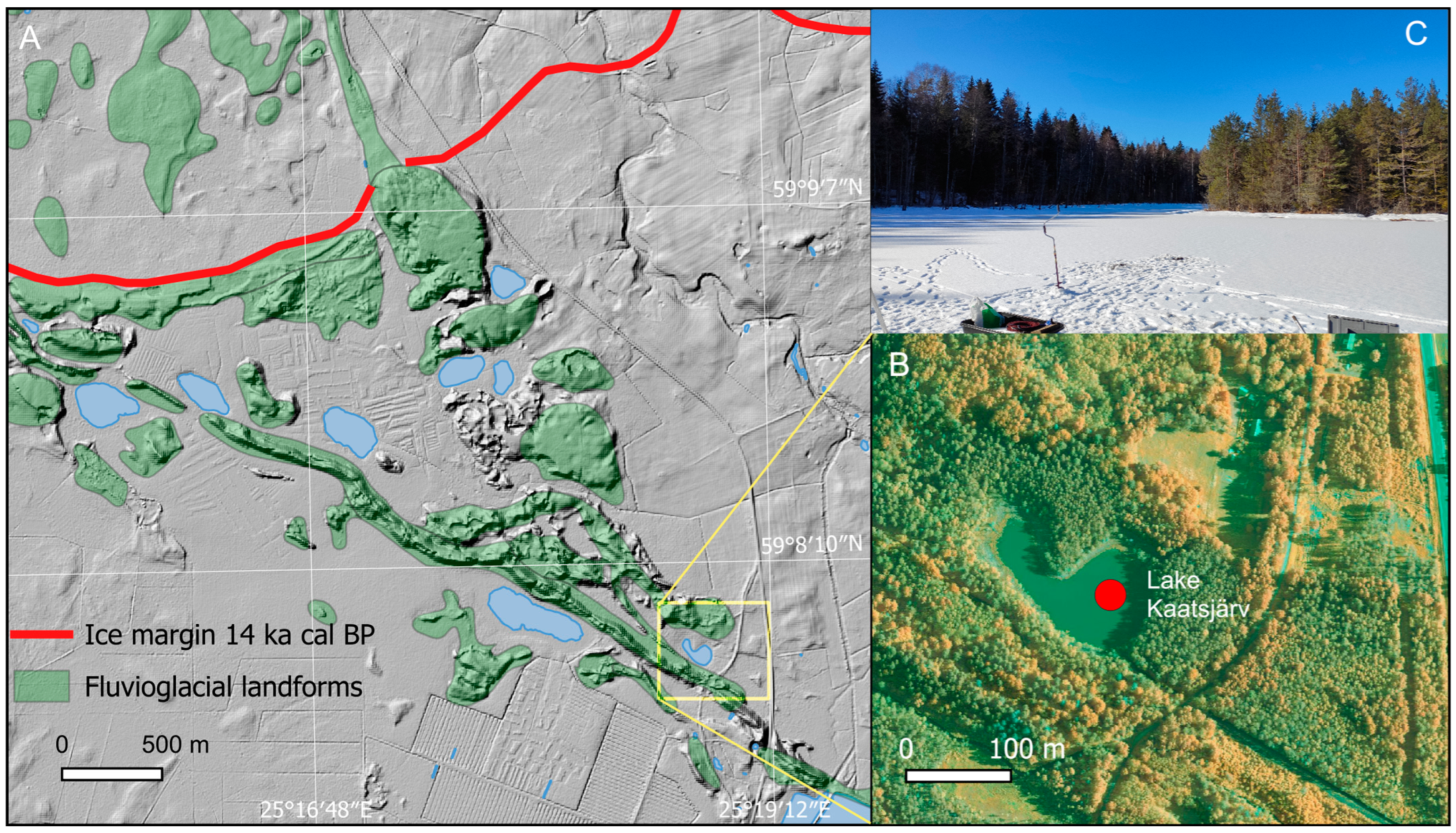
2.1. Study Area
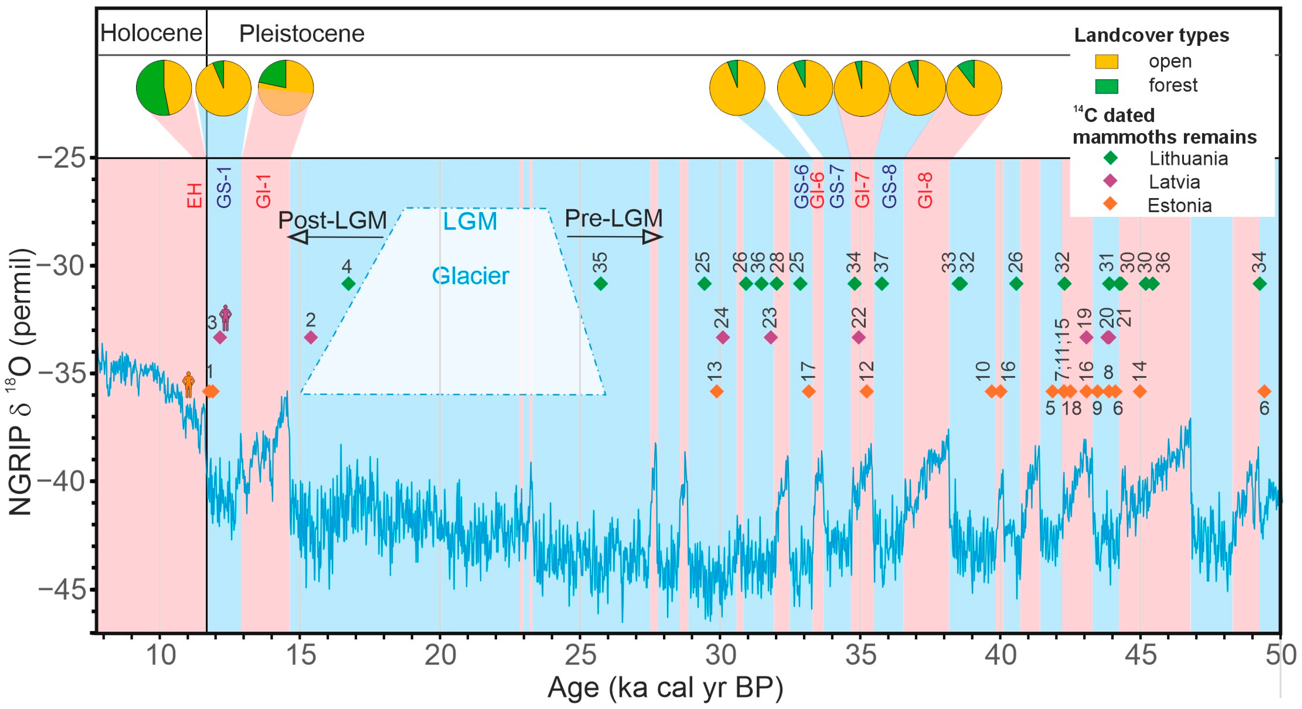
2.2. Materials

| Site | Longitude | Latitude | Lab Code | 14C age ka BP | Calibrated Ages, ka cal BP | Description | Reference | ||
|---|---|---|---|---|---|---|---|---|---|
| at 95% | Weighted Average | ||||||||
| Post-LGM | |||||||||
| Estonia | |||||||||
| 1 | Puurmani | 26.2905 | 58.5758 | Hela-423 | 10.1 ± 0.2 | 12.6–11.2 | 11.8 ± 0.36 | Molar | [1] |
| 1 | Puurmani | 26.2897 | 58.5788 | Hela-425 | 10.2 ± 0.1 | 12.5–11.4 | 11.9 ± 0.25 | Molar | [1] |
| Latvia | |||||||||
| 2 | Rucava | 21.1603 | 56.1634 | LuS 7538 | 12.88 ± 0.07 | 15.6–15.2 | 15.4 ± 0.11 | Molar | [47] |
| 3 | Rudzati | 26.453 | 56.4171 | Hela-1316 | 10.31 ± 0.07 | 12.5–11.8 | 12.2 ± 0.18 | Scapula | [47] |
| Lithuania | |||||||||
| 4 | Jiesia river | 23.8963 | 54.8952 | LuS 7529 | 13.8 ± 0.08 | 17–16.5 | 16.7 ± 0.14 | Molar | [47] |
| Pre-LGM | |||||||||
| Estonia | |||||||||
| 5 | Heimtali | 25.5002 | 58.3197 | Hela-420 | >37 | 42.1–41.7 | Tusk | [1] | |
| 6 | Ihasalu | 25.202 | 59.4971 | OxA 11563 | 46.5 ± 1 | 52.4–46.7 | 49.4 ± 1.52 | Ivory | [48] |
| 6 | Ihasalu | 25.202 | 59.4971 | Hela-426 | >41 | 44.4–43.5 | Molar | [1] | |
| 7 | Kallaste | 26.5813 | 57.6105 | Hela-421 | >38 | 42.4–42.2 | Molar | [1] | |
| 8 | Koosa | 27.0724 | 58.5116 | OxA-12058 | 40.9 ± 0.6 | 44.8–43 | 43.9 ± 0.49 | Tooth | [48] |
| 9 | Krüüdneri | 26.6959 | 58.1284 | Poz-118416 | 39.5 ± 1.3 | 45.5–41.9 | 43.5 ± 0.97 | Tusk | This study |
| 10 | Kukemetsa | 26.7619 | 58.5148 | Poz-118415 | 34.6 ± 0.7 | 41.2–37.8 | 39.7 ± 0.84 | Tusk | This study |
| 11 | Kunda | 26.54 | 59.4613 | Hela-424 | >38 | 42.4–42.2 | Tusk | [1] | |
| 12 | Mooste | 27.2209 | 58.1404 | Hela-418 | 30.64 ± 0.83 | 37.1–33.4 | 35.2 ± 0.89 | Molar | [1] |
| 13 | Rõngu | 26.2442 | 58.1435 | Poz-16733 | 25.63 ± 0.17 | 30.2–29.3 | 29.9 ± 0.22 | Humerus | [3] |
| 14 | Taagepera | 25.6921 | 57.982 | OxA-11562 | 42.2 ± 0.65 | 46.1–44 | 45 ± 0.52 | Molar | [3] |
| 15 | Tahkumägi | 26.5375 | 57.5573 | Hela-422 | >38 | 42.4–42.2 | Bone | [1] | |
| 16 | Tudulinna | 27.07 | 59.0377 | OxA 11562 | 34.81 ± 0.34 | 40.7–39.3 | 40 ± 0.36 | Ivory | [48] |
| 16 | Tudulinna | 27.07 | 59.0377 | Hela-414 | >40 | 43.3–42.9 | Tusk | [1] | |
| 17 | Valga | 26.05 | 57.78 | OxA-11607 | 28.78 ± 0.16 | 33.8–32.3 | 33.2 ± 0.36 | Tooth | [48] |
| 18 | Vitipalu | 26.4154 | 58.1652 | Poz-118499 | 38.3 ± 0.9 | 43.9–41.4 | 42.5 ± 0.56 | Tooth | This study |
| Latvia | |||||||||
| 19 | Aizpute | 21.0562 | 56.539 | Hela-1315 | >40 | 43.3–42.9 | Tusk | [3] | |
| 20 | Jaunpils | 23.013 | 56.731 | LuS 7537 | 40.7 ± 0.8 | 45–42.7 | 43.8 ± 0.6 | Molar | [47] |
| 21 | Ikšķile | 24.4976 | 56.8378 | LuS 7535 | 40.85 ± 0.75 | 45–42.8 | 43.9 ± 0.58 | Molar | [47] |
| 22 | Kalni, Nigrande | 22.1266 | 56.4466 | Hela-1314 | 30.42 ± 0.77 | 36.6–33.3 | 35 ± 0.8 | Tusk | [3] |
| 23 | Plavinas | 26.195 | 56.496 | LuS 7536 | 27.85 ± 0.2 | 32.8–31.2 | 31.8 ± 0.31 | Molar | [47] |
| 24 | Veselava | 25.398 | 57.279 | LuS 7539 | 25.8 ± 0.17 | 30.7–29.7 | 30.1 ± 0.17 | Molar | [47] |
| Lithuania | |||||||||
| 25 | Ariogala | 23.6999 | 55.4833 | FTMC-FR-48-2 | 28.633 ± 0.1 | 33.3–32.2 | 32.9 ± 0.32 | Incisivi | [49] |
| 25 | Ariogala | 23.6999 | 55.4833 | FTMC-FR-48-1 | 25.159 ± 0.09 | 29.8–29.2 | 29.4 ± 0.18 | Incisivi | [49] |
| 26 | Sviraičiai | 22.5315 | 55.9974 | RICH-22970 | 35.415 ± 0.23 | 41.1–40 | 40.6 ± 0.27 | Humerus fragment | [49] |
| 27 | Žemgrindžiai | 21.29 | 55.77 | FTMC-OZ78-1 | 26.579 ± 0.05 | 31.1–30.8 | 30.9 ± 0.08 | Tibia | [49] |
| 28 | Žagare esker | 23.2191 | 56.3511 | KIA-55701 | 27.96 ± 0.23 | 32.9–31.4 | 32 ± 0.39 | Incisivi | [49] |
| 29 | Kazokiškiai | 24.8198 | 54.8076 | OxA-10874 | 46.3 ± 1.1 | 52.4–46.2 | 49.3 ± 1.64 | Incisivi | [3] |
| 30 | Jiesia | 23.9282 | 54.858 | LuS-7531 | 42.3 ± 1 | 47.1–43.2 | 45.2 ± 0.92 | Molar | [47] |
| 30 | Jiesia | 23.9282 | 54.858 | LuS-7532 | 41.35 ± 0.8 | 45.6–43 | 44.3 ± 0.68 | Molar | [47] |
| 30 | Jiesia | 23.9282 | 54.858 | OxA-10872 | 40.9 ± 0.65 | 44.9–42.9 | 43.9 ± 0.52 | Incisivi | [3] |
| 31 | Jucaičiai | 22.1791 | 55.4522 | OxA-10870 | 40.6 ± 0.8 | 44.9–42.7 | 43.8 ± 0.59 | Molar | [3] |
| 32 | Kazokiškiai | 24.8198 | 54.8076 | OxA-10875 | 38.05 ± 0.7 | 43–41.5 | 42.3 ± 0.36 | Incisivi | [3] |
| 32 | Kazokiškiai | 24.8198 | 54.8076 | OxA-10873 | 33.74 ± 0.38 | 39.6–37.5 | 38.6 ± 0.59 | Incisivi | [3] |
| 33 | Pilsudai | 22.5133 | 55.4173 | LuS-7533 | 33.65 ± 0.3 | 39.4–37.5 | 38.5 ± 0.52 | Molar | [50] |
| 34 | Kruonis | 24.2709 | 54.7805 | OxA-10810 | 30.35 ± 0.25 | 35.3–34.4 | 34.8 ± 0.26 | Incisivi | [3] |
| 35 | Turženai | 24.0924 | 54.9838 | LuS-7528 | 21.4 ± 0.12 | 26–25.4 | 25.7 ± 0.13 | Molar | [50] |
| 36 | Olando kepure | 21.0675 | 55.7977 | Hela-3320 | 27.49 ± 0.25 | 31.9–31.1 | 31.5 ± 0.22 | Molar | [49] |
| 36 | Olando kepure | 21.0675 | 55.7977 | LuS 7918 | >43 | 45.8–45.1 | Molar | [3] | |
| 37 | Juodeliu | 23.1044 | 54.3868 | OxA-10844 | >31.4 | 36.1–35.5 | Tusk | [3] | |
2.3. Analysis of Lake Kaatsjärv Sediments
2.4. Landcover Reconstructions
| Landcover Type | Taxon | PPE (SE) | Fall Speed |
|---|---|---|---|
| Open | 2 Apiaceae | 0.21 (0.03) | 0.042 |
| 6 Artemisia | 4.33 (1.592) | 0.014 | |
| 2 Asteraceae sect. Cichorioideae | 0.07 (0.02) | 0.029 | |
| 6 Brassicaceae | 0.07 (0.04) | 0.021 | |
| 5 Calluna | 0.3 (0.03) | 0.038 | |
| 1 Caryophyllaceae | 0.6 (0.05) | 0.032 | |
| 6 Chenopodiaceae | 4.28 (0.27) | 0.019 | |
| 2 Cyperaceae | 0.13 (0.03) | 0.035 | |
| 1 Equisetum | 0.09 (0.02) | 0.021 | |
| 5 Ericaceae (incl. Empetrum nigrum and Vaccinum t.) | 0.09 (0.035) | 0.032 | |
| 1 Juniperus | 1.4 (0.05) | 0.016 | |
| Poaceae | 1 (0) | 0.035 | |
| 2 Ranunculaceae (incl. R. acris t.) | 0.08 (0.02) | 0.02 | |
| 2 Rosaceae (incl. Filipendula and Dryas octopetala) | 0.18 (0.04) | 0.022 | |
| 2 Rumex (incl. R. acetosa and R. acetosella t.) | 0.04 (0.02) | 0.018 | |
| 5 Salix | 0.09 (0.03) | 0.022 | |
| 6 Urtica | 10.52 (0.31) | 0.01 | |
| Forested | 4 Betula (incl. B. humilis and B. nana) | 2.24 (0.2) | 0.024 |
| 5 Picea | 2.8 (0.21) | 0.056 | |
| 4 Pinus | 8.4 (1.34) | 0.031 | |
| 3 Populus | 0.11 (0.09) | 0.026 |
2.5. Isotopic Analysis
3. Results
3.1. Lithology and Chronology of Kaatsjärv
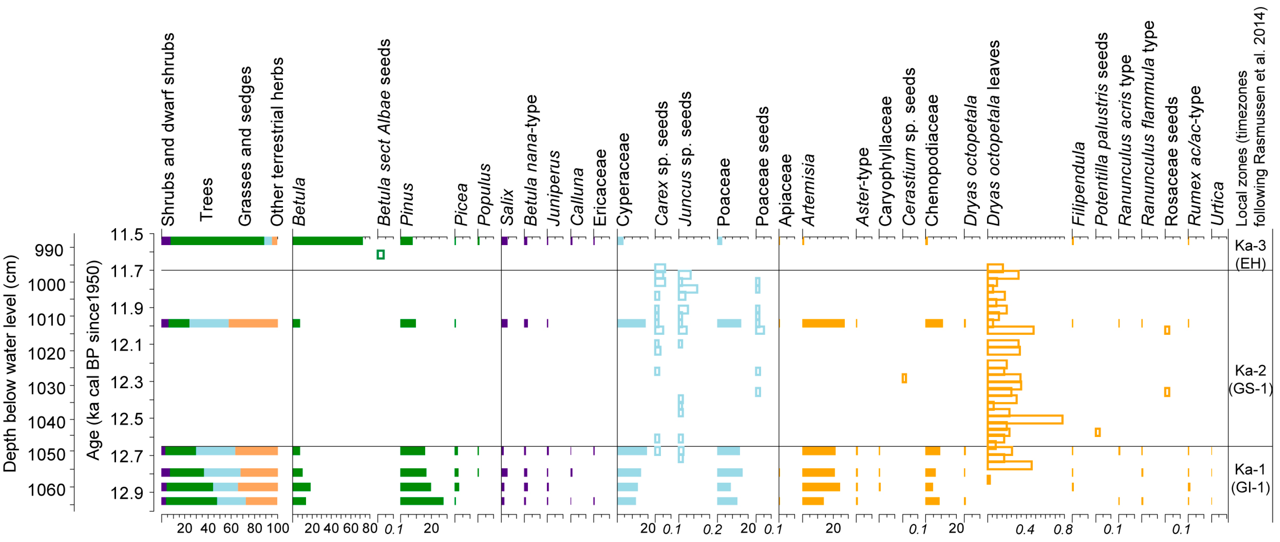
3.2. Kaatsjärv Plant Macrofossils and Pollen Diagram Description
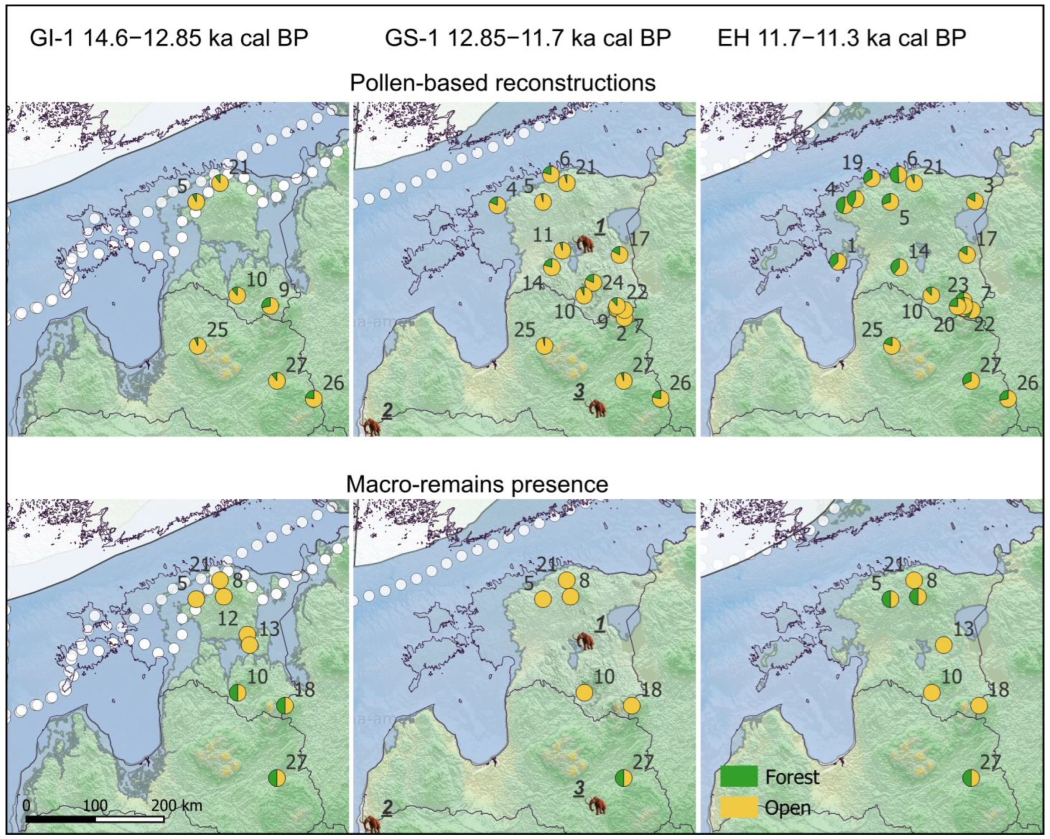
3.3. Landcover Reconstruction
3.4. Isotopic Results
4. Discussion
4.1. Landcover Reconstructions
4.2. Mammoths and Environment
4.3. Isotopic Evidence
5. Conclusions
Supplementary Materials
Author Contributions
Funding
Data Availability Statement
Acknowledgments
Conflicts of Interest
References
- Lõugas, L.; Ukkonen, P.; Jungner, H. Dating the Extinction of European Mammoths: New Evidence from Estonia. Quat. Sci. Rev. 2002, 21, 1347–1354. [Google Scholar] [CrossRef]
- Stuart, A.J. The Extinction of Woolly Mammoth (Mammuthus primigenius) and Straight-Tusked Elephant (Palaeoloxodon antiquus) in Europe. Quat. Int. 2005, 126–128, 171–177. [Google Scholar] [CrossRef]
- Ukkonen, P.; Aaris-Sørensen, K.; Arppe, L.; Clark, P.U.; Daugnora, L.; Lister, A.M.; Lõugas, L.; Seppä, H.; Sommer, R.S.; Stuart, A.J.; et al. Woolly Mammoth (Mammuthus primigenius Blum.) and Its Environment in Northern Europe during the Last Glaciation. Quat. Sci. Rev. 2011, 30, 693–712. [Google Scholar] [CrossRef]
- Guthrie, R.D. Paleoecology of the Large-Mammal Community in Interior Alaska during the Late Pleistocene. Am. Midl. Nat. 1968, 79, 346. [Google Scholar] [CrossRef]
- Kahlke, R.D. The History of the Origin, Evolution and Dispersal of the Late Pleistocene Mammuthus-Coelodonta Faunal Complex in Eurasia (Large Mammals). Quat. Sci. Rev. 2014, 96, 32–49. [Google Scholar] [CrossRef]
- Koch, P.L.; Barnosky, A.D. Late Quaternary Extinctions: State of the Debate. Annu. Rev. Ecol. Evol. Syst. 2006, 37, 215–250. [Google Scholar] [CrossRef]
- Leshchinskiy, S.V. Strong Evidence for Dietary Mineral Imbalance as the Cause of Osteodystrophy in Late Glacial Woolly Mammoths at the Berelyokh Site (Northern Yakutia, Russia). Quat. Int. 2017, 445, 146–170. [Google Scholar] [CrossRef]
- Leshchinskiy, S.V.; Burkanova, E.M. The Volchia Griva Mineral Oasis as Unique Locus for Research of the Mammoth Fauna and the Late Pleistocene Environment in Northern Eurasia. Quat. Res. 2022, 109, 157–182. [Google Scholar] [CrossRef]
- Wojtal, P. The Woolly Mammoth (Mammuthus primigenius) Remains from the Upper Palaeolithic Site Kraków Spadzista Street (B). In Proceedings of the First International Congress: The World of Elephants, Rome, Italy, 16–20 October 2001. [Google Scholar]
- Wojtal, P.; Haynes, G.; Klimowicz, J.; Sobczyk, K.; Tarasiuk, J.; Wroński, S.; Wilczyński, J. The Earliest Direct Evidence of Mammoth Hunting in Central Europe—The Kraków Spadzista Site (Poland). Quat. Sci. Rev. 2019, 213, 162–166. [Google Scholar] [CrossRef]
- Hughes, P.D.; Gibbard, P.L. A Stratigraphical Basis for the Last Glacial Maximum (LGM). Quat. Int. 2015, 383, 174–185. [Google Scholar] [CrossRef]
- Veski, S.; Amon, L.; Heinsalu, A.; Reitalu, T.; Saarse, L.; Stivrins, N.; Vassiljev, J. Lateglacial Vegetation Dynamics in the Eastern Baltic Region between 14,500 and 11,400calyrBP: A Complete Record since the Bølling (GI-1e) to the Holocene. Quat. Sci. Rev. 2012, 40, 39–53. [Google Scholar] [CrossRef]
- Estonian Environment Agency. Available online: https://www.ilmateenistus.ee/ (accessed on 7 October 2024).
- World Bank Group Climate Change Knowledge Portal. Available online: https://climateknowledgeportal.worldbank.org/country/latvia/climate-data-historical (accessed on 7 October 2024).
- Stroeven, A.P.; Hättestrand, C.; Kleman, J.; Heyman, J.; Fabel, D.; Fredin, O.; Goodfellow, B.W.; Harbor, J.M.; Jansen, J.D.; Olsen, L.; et al. Deglaciation of Fennoscandia. Quat. Sci. Rev. 2016, 147, 91–121. [Google Scholar] [CrossRef]
- Hughes, A.L.C.; Gyllencreutz, R.; Lohne, Ø.S.; Mangerud, J.; Svendsen, J.I. The Last Eurasian Ice Sheets—A Chronological Database and Time-slice Reconstruction, DATED-1. Boreas 2016, 45, 1–45. [Google Scholar] [CrossRef]
- Kalm, V.; Raukas, A.; Rattas, M.; Lasberg, K. Chapter 8—Pleistocene Glaciations in Estonia. In Quaternary Glaciations—Extent and Chronology; Ehlers, J., Gibbard, P.L., Hughes, P.D., Eds.; Developments in Quaternary Sciences; Elsevier: Amsterdam, The Netherlands, 2011; Volume 15, pp. 95–104. [Google Scholar]
- Rõuk, A.-M.; Raukas, A. Drumlins of Estonia. Sediment. Geol. 1989, 62, 371–384. [Google Scholar] [CrossRef]
- Raukas, A.; Teedumäe, A. Geology and Mineral Resources of Estonia; Estonian Academy Publishers: Tallinn, Estonia, 1997; ISBN 9985-50-185-3. [Google Scholar]
- Molodkov, A.; Bolikhovskaya, N. Palaeoenvironmental Changes and Their Chronology during the Latter Half of MIS 5 on the South-Eastern Coast of the Gulf of Finland. Quat. Int. 2022, 616, 40–54. [Google Scholar] [CrossRef]
- Molodkov, A.; Bolikhovskaya, N.; Miidel, A.; Ploom, K. The Sedimentary Sequence Recovered from the Voka Outcrops, Northeastern Estonia: Implications for Late Pleistocene Stratigraphy. Est. J. Earth Sci. 2007, 56, 47. [Google Scholar] [CrossRef]
- Rasmussen, S.O.; Bigler, M.; Blockley, S.P.; Blunier, T.; Buchardt, S.L.; Clausen, H.B.; Cvijanovic, I.; Dahl-Jensen, D.; Johnsen, S.J.; Fischer, H.; et al. A Stratigraphic Framework for Abrupt Climatic Changes during the Last Glacial Period Based on Three Synchronized Greenland Ice-Core Records: Refining and Extending the INTIMATE Event Stratigraphy. Quat. Sci. Rev. 2014, 106, 14–28. [Google Scholar] [CrossRef]
- Veski, S. Vegetation History, Human Impact and Palaeogeography of West Estonia. Pollen Analytical Studies of Lake and Bog Sediments. Striae 1998, 38, 119. [Google Scholar]
- Laul, S.; Kihno, K. Prehistoric Land Use and Settlement History on the Haanja Heights, Southeastern Estonia, with Special Reference to the Siksali-Hino Area. In Environmental and Cultural History of the Eastern Baltic Region; Miller, U., Hackens, T., Lang, V., Raukas, A., Hicks, S., Eds.; Council of Europe: Strasbourg, France, 1999; Volume 57, pp. 239–254. [Google Scholar]
- Kimmel, A.; Pirrus, R.; Raukas, A. Holocene Deposits. In LakePeipsi. Geology; Sulemees Publishers: Tallinn, Estonia, 1999; pp. 42–43. [Google Scholar]
- Poska, A. Three Pollen Diagrams from Coastal Estonia. Licentiat Thesis. KvartärgeologiskaAvdelningen 1994, 170, 40. [Google Scholar]
- Poska, A.; Saarse, L. Holocene Vegetation and Land-Use History in the Environs of Lake Kahala, Northern Estonia. Veg. Hist. Archaeobot. 1999, 8, 185–197. [Google Scholar] [CrossRef]
- Saarse, L.; Rajamäe, R. Holocene Vegetation and Climatic Change on the Haanja Heights, SE Estonia. Proc. Est. Acad. Sci. Geol. 1997, 46, 75. [Google Scholar] [CrossRef]
- Amon, L.; Saarse, L.; Vassiljev, J.; Heinsalu, A.; Veski, S. Timing of the Deglaciation and the Late-Glacial Vegetation Development on the Pandivere Upland, North Estonia. Bull. Geol. Soc. Finl. 2016, 88, 69–83. [Google Scholar] [CrossRef]
- Mäemets, H. Palynological and Radiocarbon Data on the Postglacial Vegetational History of Haanja Elevation (E.S.S.R.). In Čelovek, Rastitelnost i Pochva; Kurvits, Ü., Ed.; Estonian Academy of Sciences: Tartu, Estonia, 1983; pp. 98–111. [Google Scholar]
- Amon, L.; Veski, S.; Heinsalu, A.; Saarse, L. Timing of Lateglacial Vegetation Dynamics and Respective Palaeoenvironmental Conditions in Southern Estonia: Evidence from the Sediment Record of Lake Nakri. J. Quat. Sci. 2012, 27, 169–180. [Google Scholar] [CrossRef]
- Niinemets, E.; Poska, A.; Saarse, L. Vegetation History and Human Impact in the Parika Area, Central Estonia. Proc. Est. Acad. Sci. Geol. 2002, 51, 241. [Google Scholar] [CrossRef]
- Kihno, K.; Saarse, L.; Amon, L. Late Glacial Vegetation, Sedimentation and Ice Recession Chronology in the Surroundings of Lake Prossa, Central Estonia. Est. J. Earth Sci. 2011, 60, 147. [Google Scholar] [CrossRef]
- Saarse, L.; Veski, S.; Heinsalu, A.; Rajamäe, R.; Martma, T. Litho- and Biostratigraphy of Lake Päidre, South Estonia. Proc. Est. Acad. Sci. Geol. 1995, 44, 45. [Google Scholar] [CrossRef]
- Poska, A.; Saarse, L. Biostratigraphy and 14 C Dating of a Lake Sediment Sequence on the North-West Estonian Carbonaceous Plateau, Interpreted in Terms of Human Impact in the Surroundings. Veg. Hist. Archaeobot. 2002, 11, 191–200. [Google Scholar] [CrossRef]
- Veski, S.; Koppel, K.; Poska, A. Integrated Palaeoecological and Historical Data in the Service of Fine-resolution Land Use and Ecological Change Assessment during the Last 1000 Years in Rõuge, Southern Estonia. J. Biogeogr. 2005, 32, 1473–1488. [Google Scholar] [CrossRef]
- Sarv, A.; Ilves, E. Über Das Alter Der Holozänen Ablagerungen Im Mündungsgebiet Des Flusses Emajogi (Saviku). Eest. NSV Tead. Akad. Toim. Keem. Geol. 1975, 24, 64. (In Russian) [Google Scholar] [CrossRef]
- Amon, L.; Heinsalu, A.; Veski, S. Late Glacial Multiproxy Evidence of Vegetation Development and Environmental Change at Solova, Southeastern Estonia. Est. J. Earth Sci. 2010, 59, 151. [Google Scholar] [CrossRef]
- Kimmel, K.; Rajamäe, R.; Sakson, M. The Holocene Development of Tondi Mire, Northern Estonia: Pollen, Diatom and Chronological Studies. In Coastal Estonia. Recent Advances in Environmental and Cultural History; Hickens, T., Hicks, S., Lang, V., Miller, U., Saarse, L., Eds.; Council of Europe: Strasbourg, France, 1996; Volume 51, pp. 85–102. [Google Scholar]
- Ilves, E.; Mäemets, H. Results of Radiocarbon and Palynological Analyses of Coastal Depositsof Lakes Tuuljärv and Vaskna. In Palaeohydrology of the Temperate Zone III. Mires and Lakes; Raukas, A., Saarse, L., Eds.; Eesti NSV Teaduste Akadeemia: Tallinn, Estonia, 1987; pp. 108–130. [Google Scholar]
- Amon, L.; Saarse, L. Postglacial Palaeoenvironmental Changes in the Area Surrounding Lake Udriku in North Estonia. Geol. Q. 2010, 54, 85–94. [Google Scholar]
- Niinemets, E.; Saarse, L. Holocene Forest Dynamics and Human Impact in Southeastern Estonia. Veg. Hist. Archaeobot. 2006, 16, 1–13. [Google Scholar] [CrossRef]
- Kangur, M. Spatio-Temporal Distribution of Pollen in Lake Väike-Juusa (South Estonia) Sediments. Rev. Palaeobot. Palynol. 2009, 153, 354–359. [Google Scholar] [CrossRef]
- Stivrins, N.; Cerina, A.; Gałka, M.; Heinsalu, A.; Lõugas, L.; Veski, S. Large Herbivore Population and Vegetation Dynamics 14,600–8300 years Ago in Central Latvia, Northeastern Europe. Rev. Palaeobot. Palynol. 2019, 266, 42–51. [Google Scholar] [CrossRef]
- Heikkilä, M.; Fontana, S.L.; Seppä, H. Rapid Lateglacial Tree Population Dynamics and Ecosystem Changes in the Eastern Baltic Region. J. Quat. Sci. 2009, 24, 802–815. [Google Scholar] [CrossRef]
- Van Geel, B.; Van Der Plicht, J.; Kasse, C.; Mol, D. Radiocarbon Dates from the Netherlands and Doggerland as a Proxy for Vegetation and Faunal Biomass between 55 and 5 Ka Cal Bp. J. Quat. Sci. 2024, 39, 248–260. [Google Scholar] [CrossRef]
- Arppe, L.; Karhu, J.A. Oxygen Isotope Values of Precipitation and the Thermal Climate in Europe during the Middle to Late Weichselian Ice Age. Quat. Sci. Rev. 2010, 29, 1263–1275. [Google Scholar] [CrossRef]
- Barnes, I.; Shapiro, B.; Lister, A.; Kuznetsova, T.; Sher, A.; Guthrie, D.; Thomas, M.G. Genetic Structure and Extinction of the Woolly Mammoth, Mammuthus Primigenius. Curr. Biol. 2007, 17, 1072–1075. [Google Scholar] [CrossRef] [PubMed]
- Satkūnas, J.; Girininkas, A.; Rimkus, T.; Daugnora, L.; Grigienė, A.; Stančikaitė, M.; Slah, G.; Skuratovič, Ž.; Uogintas, D.; Žulkus, V. New 14C Data of Megafaunal Remains from Lithuania—Implications for the Palaeoenvironmental Interpretation of the Middle Weichselian. Geol. Q. 2023, 1, 3. [Google Scholar] [CrossRef]
- Arppe, L.; Aaris-Sørensen, K.; Daugnora, L.; Lõugas, L.; Wojtal, P.; Zupiņš, I. The Palaeoenvironmental Δ13C Record in European Woolly Mammoth Tooth Enamel. Quat. Int. 2011, 245, 285–290. [Google Scholar] [CrossRef]
- Ayliffe, L.K.; Lister, A.M.; Chivas, A.R. The Preservation of Glacial-Interglacial Climatic Signatures in the Oxygen Isotopes of Elephant Skeletal Phosphate. Palaeogeogr. Palaeoclimatol. Palaeoecol. 1992, 99, 179–191. [Google Scholar] [CrossRef]
- Kohn, M.J.; Cerling, T.E. Stable Isotope Compositions of Biological Apatite. Rev. Miner. Geochem. 2002, 48, 455–488. [Google Scholar] [CrossRef]
- van der Plicht, J.; Palstra, S.W.L. Radiocarbon and Mammoth Bones: What’s in a Date. Quat. Int. 2016, 406, 246–251. [Google Scholar] [CrossRef]
- Vassiljev, J.; Saarse, L. Timing of the Baltic Ice Lake in the Eastern Baltic. Bull. Geol. Soc. Finl. 2013, 85, 9–18. [Google Scholar] [CrossRef]
- Estonian Land Board, G.S. of E. Geological Base Map; 2024; Available online: https://geoportaal.maaamet.ee/eng/ (accessed on 15 September 2024).
- Heiri, O.; Lotter, A.F.; Lemcke, G. Loss on Ignition as a Method for Estimating Organic and Carbonate Content in Sediments: Reproducibility and Comparability of Results. J. Paleolimnol. 2001, 25, 101–110. [Google Scholar] [CrossRef]
- Bronk Ramsey, C. Deposition Models for Chronological Records. Quat. Sci. Rev. 2008, 27, 42–60. [Google Scholar] [CrossRef]
- Bronk Ramsey, C. Bayesian Analysis of Radiocarbon Dates. Radiocarbon 2009, 51, 337–360. [Google Scholar] [CrossRef]
- Reimer, P.J.; Austin, W.E.N.; Bard, E.; Bayliss, A.; Blackwell, P.G.; Bronk Ramsey, C.; Butzin, M.; Cheng, H.; Edwards, R.L.; Friedrich, M.; et al. The IntCal20 Northern Hemisphere Radiocarbon Age Calibration Curve (0–55 Cal KBP). Radiocarbon 2020, 62, 725–757. [Google Scholar] [CrossRef]
- Stockmarr, J. Tables with Spores Used in Absolute Pollen Analysis. Pollen Spores 1971, 13, 615–621. [Google Scholar]
- Berglund, B.E.; Ralska-Jasiveczowa, M. Pollen Analysis and Pollen Diagrams. Handbook of Holocene Palaeoecology and Palaeohydrology; Interscience: New York, NY, USA, 1986; pp. 455–484. [Google Scholar]
- Fægri, K.; Iversen, J. Textbook of Pollen Analysis, 4th ed.; John Wiley & Sons: Chichester, UK, 1989. [Google Scholar]
- Bennett, K.D.; Willis, K.J. Pollen. In Tracking Environmental Change Using Lake Sediments; Springer: Berlin/Heidelberg, Germany, 2002; pp. 5–32. [Google Scholar] [CrossRef]
- Beug, H.J. Leitfaden Der Pollenbestimmung Fur Mitteleuropa Und Angrenzende Gebiete; Publisher Verlag Friedrich Pfeil: Munich, Germany, 2004. [Google Scholar]
- Reille, M. Pollen et Spores d’Europe et d’Afrique Du Nord; Laboratoire de Botanique Historique et Palynologique, CNRS: Marseille, France, 1992. [Google Scholar]
- Chambers, F.M.; Beilman, D.W.; Yu, Z. Methods for Determining Peat Humification and for Quantifying Peat Bulk Density, Organic Matter and Carbon Content for Palaeostudies of Climate and Peatland Carbon Dynamics. Mires Peat 2011, 7, 7. [Google Scholar]
- Birks, H.H. Plant Macrofossils. In Tracking Environmental Change Using Lake Sediments; Last, W.M., Smol, J.P., Birks, H.J.B., Eds.; Kluwer: Dordrecht, The Netherlands, 2002; Volume 3, pp. 49–74. [Google Scholar]
- Katz, N.J.; Katz, S.V.; Skobeyeva, E.I. Atlas Rastitelnyh Ostatkov v Torfah (Atlas of Plant Remains in Peat); Nedra: Moscow, Russia, 1977. [Google Scholar]
- Cappers, R.T.J.; Neef, R.; Bekker, R.M. Digital Atlas of Economic Plants; Barkhuis: Groningen, The Netherlands, 2009; Volume 1. [Google Scholar]
- Grimm, E.C. Tilia and Tiliagraph. Illinois State Museum. Springfield. 1991, p. 484. Available online: https://www.neotomadb.org/apps/tilia (accessed on 14 June 2024).
- Sugita, S. Theory of Quantitative Reconstruction of Vegetation II: All You Need Is LOVE. Holocene 2007, 17, 243–257. [Google Scholar] [CrossRef]
- Theuerkauf, M.; Couwenberg, J.; Kuparinen, A.; Liebscher, V. A Matter of Dispersal: REVEALSinR Introduces State-of-the-Art Dispersal Models to Quantitative Vegetation Reconstruction. Veg. Hist. Archaeobot. 2016, 25, 541–553. [Google Scholar] [CrossRef]
- Githumbi, E.; Fyfe, R.; Gaillard, M.-J.; Trondman, A.-K.; Mazier, F.; Nielsen, A.-B.; Poska, A.; Sugita, S.; Woodbridge, J.; Azuara, J.; et al. European Pollen-Based REVEALS Land-Cover Reconstructions for the Holocene: Methodology, Mapping and Potentials. Earth Syst. Sci. Data 2022, 14, 1581–1619. [Google Scholar] [CrossRef]
- Mazier, F.; Gaillard, M.-J.; Kuneš, P.; Sugita, S.; Trondman, A.-K.; Broström, A. Testing the Effect of Site Selection and Parameter Setting on REVEALS-Model Estimates of Plant Abundance Using the Czech Quaternary Palynological Database. Rev. Palaeobot. Palynol. 2012, 187, 38–49. [Google Scholar] [CrossRef]
- Wieczorek, M.; Herzschuh, U. Compilation of Relative Pollen Productivity (RPP) Estimates and Taxonomically Harmonised RPP Datasets for Single Continents and Northern Hemisphere Extratropics. Earth Syst. Sci. Data 2020, 12, 3515–3528. [Google Scholar] [CrossRef]
- Hjelle, K.L. Herb Pollen Representation in Surface Moss Samples from Mown Meadows and Pastures in Western Norway. Veg. Hist. Archaeobot. 1998, 7, 79–96. [Google Scholar] [CrossRef]
- Räsänen, S.; Suutari, H.; Nielsen, A.B. A Step Further towards Quantitative Reconstruction of Past Vegetation in Fennoscandian Boreal Forests: Pollen Productivity Estimates for Six Dominant Taxa. Rev. Palaeobot. Palynol. 2007, 146, 208–220. [Google Scholar] [CrossRef]
- von Stedingk, H.; Fyfe, R.M. The Use of Pollen Analysis to Reveal Holocene Treeline Dynamics: A Modelling Approach. Holocene 2009, 19, 273–283. [Google Scholar] [CrossRef]
- Bunting, M.J.; Armitage, R.; Binney, H.A.; Waller, M. Estimates of ‘Relative Pollen Productivity’ and ‘Relevant Source Area of Pollen’ for Major Tree Taxa in Two Norfolk (UK) Woodlands. Holocene 2005, 15, 459–465. [Google Scholar] [CrossRef]
- Hopla, E.J. A New Perspective on Quaternary Land Cover in Central Alaska. Ph.D. Thesis, University of Southampton, Southampton, UK, 2017. [Google Scholar]
- QGIS Geographic Information System 2024. Available online: https://www.qgis.org/ (accessed on 14 June 2024).
- Bunting, M.J.; Farrell, M.; Broström, A.; Hjelle, K.L.; Mazier, F.; Middleton, R.; Nielsen, A.B.; Rushton, E.; Shaw, H.; Twiddle, C.L. Palynological Perspectives on Vegetation Survey: A Critical Step for Model-Based Reconstruction of Quaternary Land Cover. Quat. Sci. Rev. 2013, 82, 41–55. [Google Scholar] [CrossRef]
- Cersoy, S.; Zazzo, A.; Lebon, M.; Rofes, J.; Zirah, S. Collagen Extraction and Stable Isotope Analysis of Small Vertebrate Bones: A Comparative Approach. Radiocarbon 2017, 59, 679–694. [Google Scholar] [CrossRef]
- Rosentau, A.; Vassiljev, J.; Hang, T.; Saarse, L.; Kalm, V. Development of the Baltic Ice Lake in the Eastern Baltic. Quat. Int. 2009, 206, 16–23. [Google Scholar] [CrossRef]
- Ambrose, S.H. Preparation and Characterization of Bone and Tooth Collagen for Isotopic Analysis. J. Archaeol. Sci. 1990, 17, 431–451. [Google Scholar] [CrossRef]
- Ambrose, S.H. Isotopic Analysis of Paleodiet: Methodological and Interpretive Considerations, Investigation of Ancient Human Tissue: Chemical Analyses in Anthropology. Gordon Breach 1993, 10, 59–130. [Google Scholar]
- Guiry, E.J.; Szpak, P. Improved Quality Control Criteria for Stable Carbon and Nitrogen Isotope Measurements of Ancient Bone Collagen. J. Archaeol. Sci. 2021, 132, 105416. [Google Scholar] [CrossRef]
- Kelly, E.F.; Yonker, C.M. Factors of Soil Formation|Time. In Encyclopedia of Soils in the Environment; Elsevier: Amsterdam, The Netherlands, 2005; pp. 536–539. [Google Scholar]
- Stone, E.J.; Lunt, D.J. The Role of Vegetation Feedbacks on Greenland Glaciation. Clim. Dyn. 2013, 40, 2671–2686. [Google Scholar] [CrossRef]
- Amon, L.; Veski, S.; Vassiljev, J. Tree Taxa Immigration to the Eastern Baltic Region, Southeastern Sector of Scandinavian Glaciation during the Late-Glacial Period (14,500-11,700 Cal. b.p.). Veg. Hist. Archaeobot. 2014, 23, 207–216. [Google Scholar] [CrossRef]
- Sun, Y.; Xu, Q.; Gaillard, M.-J.; Zhang, S.; Li, D.; Li, M.; Li, Y.; Li, X.; Xiao, J. Pollen-Based Reconstruction of Total Land-Cover Change over the Holocene in the Temperate Steppe Region of China: An Attempt to Quantify the Cover of Vegetation and Bare Ground in the Past Using a Novel Approach. Catena 2022, 214, 106307. [Google Scholar] [CrossRef]
- Hjelmroos, M. Evidence of Long-Distance Transport of Betula Pollen. Grana 1991, 30, 215–228. [Google Scholar] [CrossRef]
- Szczepanek, K.; Myszkowska, D.; Worobiec, E.; Piotrowicz, K.; Ziemianin, M.; Bielec-Bąkowska, Z. The Long-Range Transport of Pinaceae Pollen: An Example in Kraków (Southern Poland). Aerobiologia 2017, 33, 109–125. [Google Scholar] [CrossRef] [PubMed]
- Amon, L.; Wagner-Cremer, F.; Vassiljev, J.; Veski, S. Spring Onset and Seasonality Patterns during the Late Glacial Period in the Eastern Baltic Region. Clim. Past. 2022, 18, 2143–2153. [Google Scholar] [CrossRef]
- Feurdean, A.; Perşoiu, A.; Tanţău, I.; Stevens, T.; Magyari, E.K.; Onac, B.P.; Marković, S.; Andrič, M.; Connor, S.; Fărcaş, S.; et al. Climate Variability and Associated Vegetation Response throughout Central and Eastern Europe (CEE) between 60 and 8 Ka. Quat. Sci. Rev. 2014, 106, 206–224. [Google Scholar] [CrossRef]
- Veski, S.; Seppä, H.; Stančikaite, M.; Zernitskaya, V.; Reitalu, T.; Gryguc, G.; Heinsalu, A.; Stivrins, N.; Amon, L.; Vassiljev, J.; et al. Quantitative Summer and Winter Temperature Reconstructions from Pollen and Chironomid Data between 15 and 8 Ka BP in the Baltic–Belarus Area. Quat. Int. 2015, 388, 4–11. [Google Scholar] [CrossRef]
- Alley, R.B.; Meese, D.A.; Shuman, C.A.; Gow, A.J.; Taylor, K.C.; Grootes, P.M.; White, J.W.C.; Ram, M.; Waddington, E.D.; Mayewski, P.A.; et al. Abrupt Increase in Greenland Snow Accumulation at the End of the Younger Dryas Event. Nature 1993, 362, 527–529. [Google Scholar] [CrossRef]
- Birks, H.J.B.; Birks, H.H. Biological Responses to Rapid Climate Change at the Younger Dryas—Holocene Transition at Kråkenes, Western Norway. Holocene 2008, 18, 19–30. [Google Scholar] [CrossRef]
- Guthrie, R.D. Origin and Causes of the Mammoth Steppe: A Story of Cloud Cover, Woolly Mammal Tooth Pits, Buckles, and inside-out Beringia. Quat. Sci. Rev. 2001, 20, 549–574. [Google Scholar] [CrossRef]
- Laumets, L.; Kalm, V.; Poska, A.; Kele, S.; Lasberg, K.; Amon, L. Palaeoclimate Inferred from Δ18O and Palaeobotanical Indicators in Freshwater Tufa of Lake Äntu Sinijärv, Estonia. J. Paleolimnol. 2014, 51, 99–111. [Google Scholar] [CrossRef]
- Willerslev, E.; Davison, J.; Moora, M.; Zobel, M.; Coissac, E.; Edwards, M.E.; Lorenzen, E.D.; Vestergård, M.; Gussarova, G.; Haile, J.; et al. Fifty Thousand Years of Arctic Vegetation and Megafaunal Diet. Nature 2014, 506, 47–51. [Google Scholar] [CrossRef]
- van Geel, B.; Fisher, D.C.; Rountrey, A.N.; van Arkel, J.; Duivenvoorden, J.F.; Nieman, A.M.; van Reenen, G.B.A.; Tikhonov, A.N.; Buigues, B.; Gravendeel, B. Palaeo-Environmental and Dietary Analysis of Intestinal Contents of a Mammoth Calf (Yamal Peninsula, Northwest Siberia). Quat. Sci. Rev. 2011, 30, 3935–3946. [Google Scholar] [CrossRef]
- Iacumin, P.; Nikolaev, V.; Ramigni, M. C and N Stable Isotope Measurements on Eurasian Fossil Mammals, 40 000 to 10 000 Years BP: Herbivore Physiologies and Palaeoenvironmental Reconstruction. Palaeogeogr. Palaeoclimatol. Palaeoecol. 2000, 163, 33–47. [Google Scholar] [CrossRef]
- Bocherens, H.; Drucker, D.G.; Bonjean, D.; Bridault, A.; Conard, N.J.; Cupillard, C.; Germonpré, M.; Höneisen, M.; Münzel, S.C.; Napierala, H.; et al. Isotopic Evidence for Dietary Ecology of Cave Lion (Panthera spelaea) in North-Western Europe: Prey Choice, Competition and Implications for Extinction. Quat. Int. 2011, 245, 249–261. [Google Scholar] [CrossRef]
- Zimov, S.A. Pleistocene Park: Return of the Mammoth’s Ecosystem. Science 2005, 308, 796–798. [Google Scholar] [CrossRef]
- Zagorska, I. New Testimony about Reindeer Hunters in Latvia (Jauna Liecība Par Ziemeļbriežu Medniekiem Latvijā). Latv. Vēstures Institūta Žurnāla 2010, 77, 105–112. [Google Scholar]
- Jaanits, L.; Jaanits, K. Frühmesolithische Siedlung in Pulli. Eest. NSV Tead. Akad. Toim. Ühiskonnateadused 1975, 24, 64–70. [Google Scholar] [CrossRef]
- Lõugas, L. Post-Glacial Development Ofvertebrate Fauna in Estonian Water Bodies; A Palaeozoological Study; Dissertationes Biologicae Universitatis: Tartu, Estonia, 1997. [Google Scholar]
- Poska, A.; Veski, S. Man and Environment at 9500 Bp. A Palynological Study of an Early-Mesolithic Settlement Site in South-West Estonia. Acta Palaeobot. 1999, S2, 603–607. [Google Scholar]
- Wooller, M.J.; Zazula, G.D.; Edwards, M.; Froese, D.G.; Boone, R.D.; Parker, C.; Bennett, B. Stable Carbon Isotope Compositions of Eastern Beringian Grasses and Sedges: Investigating Their Potential as Paleoenvironmental Indicators. Arct. Antarct. Alp. Res. 2007, 39, 318–331. [Google Scholar] [CrossRef]
- Kilgallon, C.; Flach, E.; Boardman, W.; Routh, A.; Strike, T.; Jackson, B. Analysis of Biochemical Markers of Bone Metabolism in Asian Elephants (Elephas maximus). J. Zoo Wildl. Med. 2008, 39, 527–536. [Google Scholar] [CrossRef] [PubMed]
- van der Merwe, N.J.; Thorp, J.A.L.; Bell, R.H.V. Carbon Isotopes as Indicators of Elephant Diets and African Environments. Afr. J. Ecol. 1988, 26, 163–172. [Google Scholar] [CrossRef]
- Bocherens, H. Isotopic Tracking of Large Carnivore Palaeoecology in the Mammoth Steppe. Quat. Sci. Rev. 2015, 117, 42–71. [Google Scholar] [CrossRef]
- van der Merwe, N.J. Carbon Isotopes, Photosynthesis, and Archaeology: Different Pathways of Photosynthesis Cause Characteristic Changes in Carbon Isotope Ratios That Make Possible the Study of Prehistoric Human Diets. Am. Sci. 1982, 70, 596–606. [Google Scholar]
- Ambrose, S.H.; DeNiro, M.J. The Isotopic Ecology of East African Mammals. Oecologia 1986, 69, 395–406. [Google Scholar] [CrossRef]
- van der Merwe, N.J.; Medina, E. The Canopy Effect, Carbon Isotope Ratios and Foodwebs in Amazonia. J. Archaeol. Sci. 1991, 18, 249–259. [Google Scholar] [CrossRef]
- Amundson, R.; Austin, A.T.; Schuur, E.A.G.; Yoo, K.; Matzek, V.; Kendall, C.; Uebersax, A.; Brenner, D.; Baisden, W.T. Global Patterns of the Isotopic Composition of Soil and Plant Nitrogen. Glob. Biogeochem. Cycles 2003, 17, 31. [Google Scholar] [CrossRef]
- Zimov, S.A.; Zimov, N.S.; Tikhonov, A.N.; Chapin, F.S. Mammoth Steppe: A High-Productivity Phenomenon. Quat. Sci. Rev. 2012, 57, 26–45. [Google Scholar] [CrossRef]
- Owen-Smith, N. Pleistocene Extinctions: The Pivotal Role of Megaherbivores. Paleobiology 1987, 13, 351–362. [Google Scholar] [CrossRef]
- Austrheim, G.; Eriksson, O. Recruitment and Life-History Traits of Sparse Plant Species in Subalpine Grasslands. Can. J. Bot. 2003, 81, 171–182. [Google Scholar] [CrossRef]
- Güsewell, S. N:P Ratios in Terrestrial Plants: Variation and Functional Significance. New Phytol. 2004, 164, 243–266. [Google Scholar] [CrossRef]
- Cornelissen, J.H.C.; Quested, H.M.; Gwynn-Jones, D.; Van Logtestijn, R.S.P.; De Beus, M.A.H.; Kondratchuk, A.; Callaghan, T.V.; Aerts, R. Leaf Digestibility and Litter Decomposability Are Related in a Wide Range of Subarctic Plant Species and Types. Funct. Ecol. 2004, 18, 779–786. [Google Scholar] [CrossRef]
- Michelsen, A.; Quarmby, C.; Sleep, D.; Jonasson, S. Vascular Plant 15 N Natural Abundance in Heath and Forest Tundra Ecosystems Is Closely Correlated with Presence and Type of Mycorrhizal Fungi in Roots. Oecologia 1998, 115, 406–418. [Google Scholar] [CrossRef] [PubMed]
- Drucker, D.G.; Stevens, R.E.; Germonpré, M.; Sablin, M.V.; Péan, S.; Bocherens, H. Collagen Stable Isotopes Provide Insights into the End of the Mammoth Steppe in the Central East European Plains during the Epigravettian. Quat. Res. 2018, 90, 457–469. [Google Scholar] [CrossRef]


| Site Number | Site | Longitude | Latitude | Analyses | Time Periods | Reference | ||
|---|---|---|---|---|---|---|---|---|
| EH | GS-1 | GI-1 | ||||||
| Post-LGM sites | ||||||||
| 1 | Ermistu | 23.9829 | 58.3572 | Pollen | + | [23] | ||
| 2 | Hino | 27.2386 | 57.5831 | Pollen | + | [24] | ||
| 3 | Imatu | 27.4611 | 59.0997 | Pollen | + | [25] | ||
| 4 | Järveotsa | 24.1542 | 59.0956 | Pollen | + | + | [26] | |
| 5 | Kaatsjärv | 25.3141 | 59.1318 | Pollen, Macro | + | + | + | This study |
| 6 | Kahala | 25.5315 | 59.4867 | Pollen | + | + | [27] | |
| 7 | Kirikumäe | 27.2522 | 57.6830 | Pollen | + | + | [28] | |
| 8 | Kursi | 26.0156 | 59.1558 | Macro | + | + | + | [29] |
| 9 | Mäetilga | 27.0719 | 57.7420 | Pollen | + | + | + | [30] |
| 10 | Nakri | 26.2731 | 57.8951 | Pollen, Macro | + | + | + | [31] |
| 11 | Parika | 25.7742 | 58.4903 | Pollen | + | [32] | ||
| 12 | Prossa | 26.5778 | 58.6492 | Macro | + | [33] | ||
| 13 | Pupastvere | 26.6239 | 58.5115 | Macro | + | + | This study | |
| 14 | Päidre | 25.5033 | 58.2761 | Pollen | + | + | [34] | |
| 15 | Ruila | 24.4297 | 59.1758 | Pollen | + | [35] | ||
| 16 | Rõuge | 26.905 | 57.7389 | Pollen | + | [36] | ||
| 17 | Saviku | 27.1940 | 58.4062 | Pollen | + | + | [37] | |
| 18 | Solova | 27.4280 | 57.7004 | Macro | + | + | + | [38] |
| 19 | Tondi | 24.8533 | 59.4450 | Pollen | + | [39] | ||
| 20 | Tuuljärv | 27.0556 | 57.7056 | Pollen | + | + | [40] | |
| 21 | Udriku | 25.9315 | 59.3719 | Pollen, Macro | + | + | + | [41] |
| 22 | Vaskna | 27.0783 | 57.7117 | Pollen | + | + | [40] | |
| 23 | Verijärv | 27.0583 | 57.8083 | Pollen | + | [42] | ||
| 24 | Väike_Juusa | 26.5172 | 58.0592 | Pollen | + | [43] | ||
| 25 | Āraiši | 25.2828 | 57.2514 | Pollen | + | + | + | [44] |
| 26 | Kurjanovas | 28 | 56.5 | Pollen | + | + | + | [45] |
| 27 | Lielais Svētiņu | 27.1491 | 56.7591 | Pollen, Macro | + | + | + | [12] |
| Depth, from the Lake Water Surface, cm | Lab Code | 14C age ka BP | Modelled Ages ka cal BP | Remark | Dated Material | |
|---|---|---|---|---|---|---|
| At 95.4% Probability Range | Weighted Average | |||||
| 1015 | Poz-173419 * | 11.8 ± 0.07 | 14.0–13.5 | 13.7 ± 0.09 | 0.3 mgC | Dryas octopetala leaves unidentified stems and leaves |
| 1040 | Poz-173420 | 10.5 ± 0.120 | 12.6–12.4 | 12.5 ± 0.06 | 0.08 mgC | Dryas octopetala leaves unidentified stems and leaves |
| 1050 | Poz-173421 | 10.6 ± 0.07 | 12.8–12.6 | 12.7 ± 0.04 | 0.18 mgC | Dryas octopetala leaves unidentified stems and leaves |
| 1058–1068 | Poz-81832 | 11 ± 0.06 | 13.1–12.8 | 12.9 ± 0.07 | Bulk sediment | |
| Sample ID | Material | δ15N (‰) ± SD | δ13C (‰) ± SD | N | C | C:N |
|---|---|---|---|---|---|---|
| KRÜ | Mammoth molar | +9.8 | −21.1 | 1.1 | 3.6 | 3.1 |
| KUK | Mammoth molar | +10.1 ± 0.02 | −20.6 ± 0.05 | 1.0 | 3.6 | 3.3 |
| TAM G441:47 | Mammoth molar | +7.4 ± 0.09 | −20.2 ± 0.4 | 0.5 | 2.3 | 4.1 |
| TAM G441:48 | Mammoth molar | +6.5 ± 0.9 | −21.2 ± 0.9 | 0.9 | 2.5 | 2.7 |
Disclaimer/Publisher’s Note: The statements, opinions and data contained in all publications are solely those of the individual author(s) and contributor(s) and not of MDPI and/or the editor(s). MDPI and/or the editor(s) disclaim responsibility for any injury to people or property resulting from any ideas, methods, instructions or products referred to in the content. |
© 2025 by the authors. Licensee MDPI, Basel, Switzerland. This article is an open access article distributed under the terms and conditions of the Creative Commons Attribution (CC BY) license (https://creativecommons.org/licenses/by/4.0/).
Share and Cite
Krivokorin, I.; Poska, A.; Vassiljev, J.; Veski, S.; Amon, L. Environment of European Last Mammoths: Reconstructing the Landcover of the Eastern Baltic Area at the Pleistocene/Holocene Transition. Land 2025, 14, 178. https://doi.org/10.3390/land14010178
Krivokorin I, Poska A, Vassiljev J, Veski S, Amon L. Environment of European Last Mammoths: Reconstructing the Landcover of the Eastern Baltic Area at the Pleistocene/Holocene Transition. Land. 2025; 14(1):178. https://doi.org/10.3390/land14010178
Chicago/Turabian StyleKrivokorin, Ivan, Anneli Poska, Jüri Vassiljev, Siim Veski, and Leeli Amon. 2025. "Environment of European Last Mammoths: Reconstructing the Landcover of the Eastern Baltic Area at the Pleistocene/Holocene Transition" Land 14, no. 1: 178. https://doi.org/10.3390/land14010178
APA StyleKrivokorin, I., Poska, A., Vassiljev, J., Veski, S., & Amon, L. (2025). Environment of European Last Mammoths: Reconstructing the Landcover of the Eastern Baltic Area at the Pleistocene/Holocene Transition. Land, 14(1), 178. https://doi.org/10.3390/land14010178