Abstract
Based on the perspective of financial geography, this study analyzed the convergent mechanism of urban–rural financial imbalances under the influence of spatial spillover through the theoretical framework of spatial process, spatial action, and spatial convergence. Then, we empirically tested the spatial spillover, spatial difference, and spatial convergence of urban–rural financial imbalances in China from 1991 to 2021. We found that urban–rural financial imbalances showed significant spillover effects and heterogeneous characteristics. Spillovers based on financial radiation and exclusion were apparent during the urban financial agglomeration stage, decreasing with geographical distance, and had an essential impact on the convergence of provincial urban–rural financial imbalance. As such spillovers declined during the financial diffusion period, new spillovers at the technology and information dimensions, which were less geographically constrained, came into play and contributed to urban–rural financial convergence. The policy implications are that it is necessary to pay attention to the spatial interaction of urban–rural financial inequality, correctly use their spillover effects to achieve financial convergence, and activate new spatial spillover channels according to their spatial interaction mode changes for further urban and rural financial convergence.
1. Introduction
Sustainable development of finance refers to the rational development and utilization of financial resources in the long term. Unbalanced operation of financial resources such as underdevelopment or over-development in a certain period is not sustainable [1]. Financial convergence is an inevitable requirement to alleviate the unbalanced allocation of urban and rural financial resources. Urban–rural financial imbalances are formed in the spatial process of urban financial agglomeration and diffusion. At the beginning of the 1990s, market-oriented reforms of the financial system opened channels of cross-regional flow of financial resources in China. During the process, financial resources mainly flowed from rural to urban areas and concentrated in the core cities, beginning the process of urban financial agglomeration. Financial institutions continued to expand into the surrounding areas under the effect of circular cumulative causation, forming different levels of financial centers in the surrounding areas during the leap of each stage. Eventually, a multi-level financial center network came into being, generating spatial spillover effects [2]. Financial agglomeration zones absorb financial resources from the surroundings and positively spill over to the periphery through trickle-down effects, such as setting up branches, disseminating technology, and managing experience [3]. They can affect financial supply in peripheral rural areas by improving capital availability. On the other hand, areas with a large amount of financial outflow will have a high level of financial exclusion, which inhibits the financial supply for surrounding rural areas. When financial resources in the core city become saturated and spread to the periphery, the magnitude of these spillovers changes with the intensity of financial diffusion. Therefore, spatial spillovers play an important role in converging urban–rural financial imbalance. How do these spillover effects form and manifest during urban financial agglomeration and diffusion? Are they heterogeneous in different regions? What are urban–rural financial inequality’s convergent mechanism and bottleneck under spatial spillovers? The study of the above questions is vital for the coordinated development of urban and rural finance from a perspective of spatial synergy.
The existing studies mainly focus on converging urban and rural finance from a non-spatial perspective. Most research has paid attention to the narrowing of urban and rural financial differences. According to the neoclassical development theory, marginal capital returns drive the flow of financial resources and converge urban–rural finance in various regions. However, information asymmetry in rural credit markets leads to adverse selection and moral hazards, thus causing market failure [4,5]. Governments also play exogenous roles through urban preferences or intervention in bank credit [6,7]. Therefore, large amounts of financial resources flow from rural to urban areas, with the fiscal and financial systems playing an important role in withdrawing rural funds [8,9]. The reverse outflow of rural financial resources makes the gaps in urban–rural finance persist, which are reflected in financial assets, financial loans, and financial development, etc. [10,11].
Moreover, the imbalance between urban and rural financial development is also reflected at the regional level. Inter-provincial inequality is evident and sustainable in the three regions and eight economic zones [12]. Urban–rural financial imbalances among the eastern, central, and western areas are slight, while within the regions they are considerable, especially in eastern provinces [13]. However, Jiang and Xie believe that expanding urban–rural financial imbalance is only temporary. When urban financial development reaches a certain threshold, it will promote the development of rural finance and narrow the gap between urban and rural finance. This effect is pronounced in the eastern region but has yet to appear in the central and western areas [11]. Research on the convergence of urban–rural financial imbalance in different provinces is rare. Li argues that urban–rural financial imbalances in China have shown a conditional convergence trend and have club convergence characteristics [14].
The above discussions are based on the neoclassical theory hypothesis, which considers provincial urban–rural financial differences as independent entities without spatial spillovers. However, regional interactions should be addressed. The research perspective of financial geography emphasizes the information-based geographical attributes of financial activities, describes spatial factors’ influences on financial activities, and explains the formation of financial agglomeration and financial exclusion as well as their spatial spillover effects [15,16,17]. Spatial interactions are conducive to helping undeveloped regions catch up with developed areas and realize convergence [18]. Therefore, spatial dependence and heterogeneity have become practical problems in cross-sectional and spatial-temporal analyses [19], as various spillover effects due to factor mobility, transfer payments, and technological diffusion become operational [20]. Ignoring spillover effects will lead to bias in the convergence model setting [21]. Models with spatial spillover have been widely used in the convergence study of China’s economic growth and financial development [22,23,24,25].
In fact, within the linked network of regional economies, urban–rural development also exhibits spatial heterogeneity and dependence. In spatial agglomeration, urban systems gradually self-organize into a highly regular hierarchy and form a connected network structure [26,27,28]. Symbiotic relationships can emerge between urban hierarchies based on regional market potential, including the rural fringe [26,29]. The positive externalities of urban development for rural areas show spatial agglomeration characteristics, with counties near large cities such as Beijing, Shanghai, Guangzhou, and Shenzhen having higher agricultural labor productivity from 2000 to 2010 [30]. Urban–rural integration has a positive spatial correlation, and the agglomeration effects of cities play a dominant role [31]. The agglomeration and diffusion of economic and financial resources enhance the spatial interaction of urban–rural financial differences, making their evolution and convergence exhibit new characteristics. Regarding spatial logic, urban–rural integrated development involves reconstructing urban–rural spatial relations [32]. Therefore, the spatial effect is a prerequisite that cannot be ignored when studying the convergence of urban–rural financial differences. However, no spatial effects of urban–rural financial imbalance are considered in the existing literature, motivating us to pursue this topic.
The aim of this paper is to explore the convergence of urban–rural financial imbalances under spatial spillover effects formed during urban financial agglomeration and diffusion. Its contributions are as follows. Firstly, we construct an analytic framework to elaborate on the influence of spatial spillovers on convergence through the financial geographical perspective of spatial process, spatial action, and spatial convergence. Secondly, we demonstrate the existence of spillovers among provincial urban–rural financial imbalances, including spillovers based on financial radiation and financial exclusion. Thirdly, we examine the convergent mechanism of urban–rural financial imbalance under spatial spillover effects. Finally, we propose policies for convergence and sustainable development of urban and rural finance from a perspective of spatial coordination. We found that urban–rural financial differences show significant spillover effects and heterogeneous characteristics. Spillovers based on financial radiation and exclusion were obvious during urban financial agglomeration. The former was conducive, while the latter was detrimental to convergence. Both decreased with geographical distance and weakened during the financial diffusion phase. At this time, spatial spillovers in the information and technology dimensions less constrained by geographical distance become obvious and played a positive role in converging urban–rural financial imbalances in the middle and western areas. Therefore, it is necessary to stimulate new spillover channels to promote the further convergence of urban–rural financial disequilibrium.
2. Theories and Hypotheses
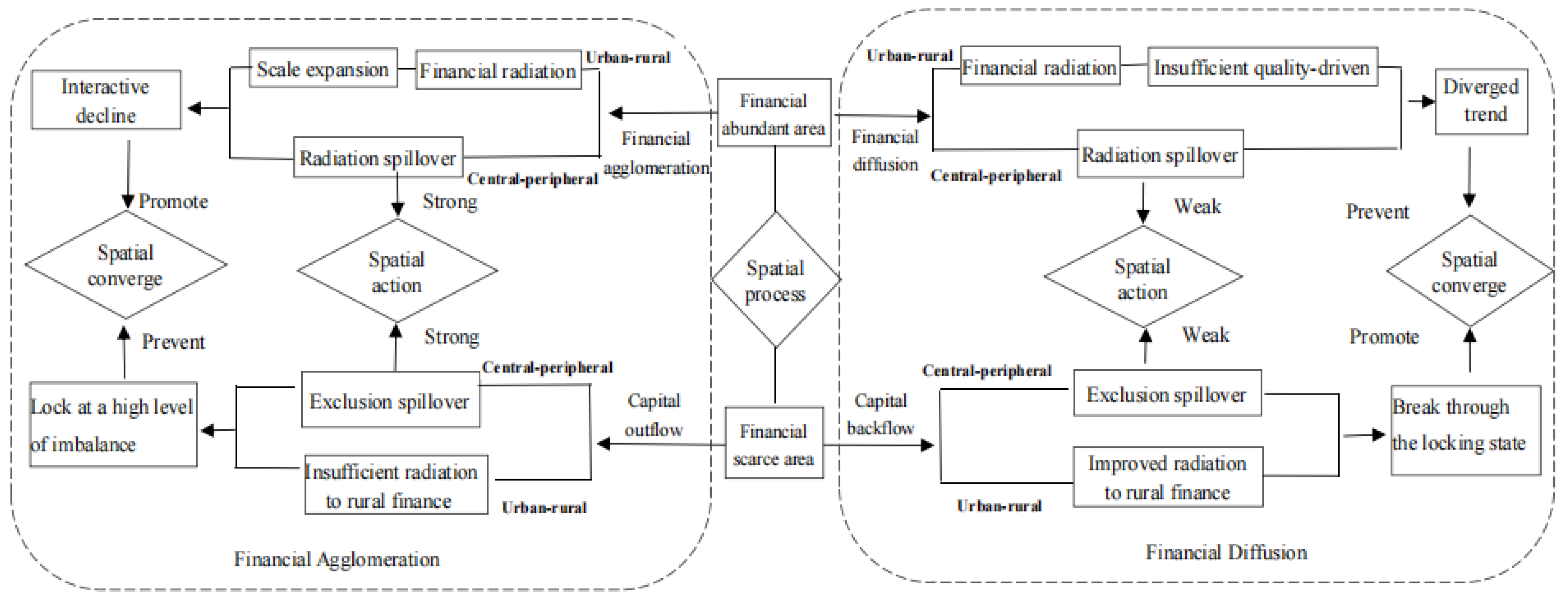
Figure 1 describes spatial spillovers and the convergence of urban–rural financial imbalances. Our analytical logic was based on the perspective of financial geography, which contains spatial differences, spatial processes, and spatial interactions [33]. As shown in Figure 1, we extended the logical chain to spatial convergence. The left and right dashed square boxes indicate the financial agglomeration and diffusion processes, respectively. The upper and lower sides are the financially abundant areas and financially scarce areas, respectively. The spatial processes are the agglomeration and diffusion of financial resources, during which financial abundant areas and scarce areas are formed. The spatial interactions are spillovers produced in the process of financial agglomeration and diffusion. Spatial convergence is the evolution trend of urban–rural financial imbalance, which is affected by spatial spillovers, and shows different characteristics in financially abundant and scarce areas. We will elaborate on the mechanism in detail.
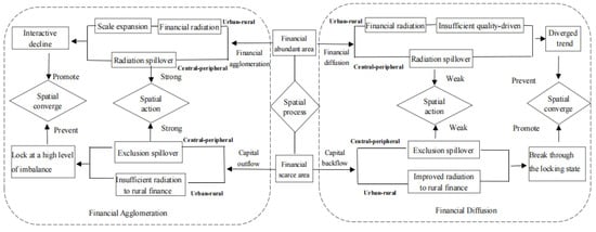
Figure 1.
Convergence of urban–rural financial imbalances under spatial spillover effects. Notes: Drawn by the author.
2.1. Financial Agglomeration, Spatial Spillovers and Convergence of Urban–Rural Financial Imbalances
Financial centers benefit from financial agglomeration, and their urban areas take the lead in radiating rural finance through the following channels: firstly, by expanding urban financial services to rural areas through financial division. Core cities continuously expand their financial scale in the cycle of cumulative causality. The externality drives the deepening of financial specialization, significantly reducing financial transaction costs and penetrating financial services to rural areas through financial expansion. Secondly, spillovers of financial talents to rural areas are promoted through a shared labor market. Financial agglomeration is conducive to fostering multi-level professional financial talents and forming a shared financial labor market. The accumulation of financial knowledge and skills generated by financial aggregation can radiate to rural areas through labor mobility, improving the human capital of rural finance. Thirdly, the asymmetry of the rural credit market is reduced through information spillovers. Competition and cooperation of core and surrounding cities form a complex horizontal and vertical connection, which enables them to form an interdependent network [34]. Rural financial institutions close to financial centers can enjoy the externalities of the above information network, significantly enhancing their access to financial services. Fourthly, rural financial innovation is promoted through spillovers of technology. Transaction costs associated with information asymmetry in rural credit markets, including information collection costs, loan monitoring costs, and disposal costs, are high, and a combination of credit techniques is needed to reduce information asymmetry [5]. As a result, it is difficult for traditional financial services to meet their financial demands, and financial innovation is required. Technical spillovers from financial centers promote adjacent rural financial institutions to provide innovative financial services suitable for rural production and operation, which better meets the diversified financial needs of rural operators and improves rural financial supply.
On the other hand, financial agglomeration strengthens the spatial spillover of urban–rural financial imbalances and contributes to their convergence. The forward and backward linkages of financial activities form close spatial interactions between cities and generate spatial spillovers through spatial demonstration, training, competition, and collaboration effects [35]. Core cities play demonstrative roles in financial products, services, and technology. This also results in spillovers of financial knowledge and management experience through training and the exchange of financial talents. Fierce market competition improves the quality of financial innovation and service in core areas. Financial institutions in various regions strengthen spatial correlation in labor specialization and spatial cooperation. Therefore, financial centers drive financial developments of peripheral areas through spatial spillover. The financial development of peripheral cities further radiates into surrounding rural areas by improving financial services, financial talents, financial information, and financial knowledge. Thus, urban–rural financial imbalance in financial abundant areas declines interactively. Spillovers based on financial radiation make peripheral areas with initially high urban–rural financial imbalance share the financial achievements of financial centers and reduce urban–rural inequality faster. As a result, financial radiation from urban to rural areas and spillover effects contribute to the convergence of urban–rural financial imbalances in financial abundant areas, as shown by the top left of Figure 1.
For financially scarce zones, an outflow of financial resources prevents the accessibility, availability, and usage of financial resources, thus inducing financial exclusion [36]. In addition, financial exclusion has a significant spatial dependence [37]. A province with high financial exclusion results in both it and adjacent provinces having a low financial availability, which makes urban finance insufficient to drive rural finance. Compared with the interacted contraction of urban–rural financial imbalances in financially abundant areas, urban–rural financial inequality in financially scarce areas will be locked at a high level. Thus, the convergence of urban–rural financial imbalances in financially scarce areas is prevented by insufficient financial radiation and exclusion spillovers, as shown by the bottom left of Figure 1. We propose two hypotheses according to the convergence characteristic during financial agglomeration.
Hypothesis 1.
Urban–rural financial imbalances have radiation spillovers and exclusion spillovers which decrease with geographical distance, with spatial dependence and spatial heterogeneity based upon them.
Hypothesis 2.
Radiation spillovers in financially abundant areas promote the convergence of urban–rural financial imbalance, while exclusion spillovers in financially scarce areas prevent it.
2.2. Financial Diffusion, Spatial Spillovers, and Convergence of Urban–Rural Financial Imbalances
When the development of urban finance in the financial abundance zone has reached a certain level, financial diffusion becomes the primary form of financial connection with the surrounding areas and starts the period of financial diffusion. At this time, failure to break through some of the relevant constraints will prevent the convergence of urban–rural financial disequilibrium in financial abundance.
Firstly, financial radiation from urban to rural areas needs to be enhanced. During financial agglomeration, rural finance has just developed from a primary stage. As a result, financial radiation from urban to rural areas is mainly based on expanding financial institutions and financial services, which promotes rural financial development through “scale expansion”. By contrast, new types of rural financial institutions gradually emerge at the stage of financial diffusion, and innovation in rural financial services is increasing. Accordingly, the effects of financial radiation need to shift from “scale expansion” to “quality-driven”, that is to say, promoting innovation and financial efficiency in rural financial services through the diffusion of financial technology. Otherwise, it will be challenging to meet the financial needs of modern agricultural production and operation, thus inhibiting radiation effects from urban to rural areas.
Secondly, spatial spillover needs to break through the spatial distance constraint of geographical proximity and spill over to regions with similar levels of information and technology. The “spread” effects are weaker compared with the “backwash” effects under market forces [38]. Furthermore, financial diffusion can also be limited by local protection and the infrastructure level of the area receiving the financial resource backflow. Insufficient financial diffusion can weaken interactions between cities, inducing a divergent trend and a decline in the convergence of urban and rural financial inequality. Spatial spillover dividends based on geographical distance have gradually been released in the financial agglomeration stage. New spatial penetration channels with less geographical constraints must be explored to maintain further convergence. In summary, the lack of “quality-driven” financial radiation from urban to rural areas and the decreased spillover effects prevent the convergence of urban–rural financial imbalance among geographically adjacent provinces, as shown in the upper right part of Figure 1.
On the other hand, financially scarce areas absorb financial resources flowing back from financially abundant regions. The quantity-oriented financial radiation from urban to rural areas increases with the enrichment of financial supply. Agglomeration of provinces with high urban–rural financial inequalities can be alleviated due to weakened financial exclusion spillovers. The breakthrough of the locking state of high urban–rural financial imbalance promotes spatial convergence in financially scarce areas, as shown by the bottom right of Figure 1. We propose hypothesis 3 based on the spatial spillover effects and convergence during financial diffusion.
Hypothesis 3.
Weakened financial radiation spillovers prevent the convergence of urban–rural financial imbalance in financially abundant areas. In contrast, improved financial radiation and weakened exclusion spillover promote convergence in financially scarce regions.
3. Methodology
3.1. Model Construction
3.1.1. The Calculation of Theil Index
We describe the spatial movement of urban financial resources and the evolution of urban–rural financial imbalance by calculating the Theil index. Let represent the whole China, China’s eastern, central, and western regions, respectively. We decomposed the total difference in region P into intra-group difference Ipwd and inter-group difference Ipbd. The former describes financial differences within urban or rural areas, as shown in Equation (1). Tloanp is the total loans of financial institutions in region P. Ip1 (IP2) is the Theil index of rural (urban) areas in region P. Tloanp1 (Tloanp2) represents the total loans of financial institutions of rural (urban) areas in region P.
The Theil index of urban areas (IP2) describes the financial differences in urban areas, as shown in Equation (2). Financial agglomeration increases urban financial differences and improves Ip2, while financial diffusion reduces it. Tloanpi2 and Laborpi2 represent the loans of financial institutions and employed population in urban areas of i province in region P, respectively. LaborP2 represents the employed population in urban areas in region P.
The inter-group difference describes financial differences between urban and rural areas, which is calculated in Equation (3). Laborp1 is the employed population in rural areas in region P. Laborp is the employed population in region P.
3.1.2. Spatial Autocorrelation Test
The Moran’s ’I index is used to test the overall spatial correlation of urban–rural financial imbalance, which is calculated as shown in Equation (4).
, where yi represents the urban–rural financial imbalance in province i, n represents the number of provinces, and Wij represents the spatial weight
The calculation of adjacent weight W1 is expressed in Equation (5). As described by Equation(6), geographical weight W2 is expressed as the reciprocal of the distance between geographical centers of two provinces represented by and . Similarly, economic weight is expressed as the reciprocal of economic distance, which is the absolute value of the difference between the average per capita real GDP of two provinces [39]. The product of adjacent weight and economic weight is spatial weight W3.
3.1.3. Spatial Econometric Model
The classical β convergence model of Barrow and Martin (1992) is shown in Equation (7) [40], where, Urdi,t0 and Urdi,t0+T represent the urban–rural financial imbalance in t0 and t0+T of i province. T is the period span, and is the random disturbance term. β represents the convergence coefficient, where β = −(1 − e−θT)/T. If β < 0, it shows that urban–rural financial imbalance tends to converge in the period of (t0, t0+T). If β > 0, it tends to diffuse.
According to the different spatial action forms of urban–rural financial imbalance, a spatial autoregressive model (SAR) and a spatial error model (SEM) are established to analyze the spatial conditional convergence. The SAR model is shown in Equation (8), and the SEM model is shown in Equations (9) and (10), respectively. In the following equations, is the spatial weight matrix. Spatial regressive coefficient ρ measures the influence of urban–rural financial imbalance of neighboring provinces to the local province. The spatial error coefficient λ measures the influence of the random disturbance of urban–rural financial imbalance in neighboring provinces on the local province. µit is a normally distributed random error vector. LnUrdi,t0 is the core explanatory variable, and Xit is the set of control variables, with the meanings shown in Table 1.

Table 1.
Variable definitions and summary descriptions.
3.2. Variables Selection
3.2.1. Dependent Variable
The dependent variable is Gur, the average annual growth rate of urban–rural financial imbalance. We calculated the urban–rural financial imbalance (Urd) at year t0+T and t0 respectively, taking the nature logarithm of their ratios, then dividing by the time interval [40].
3.2.2. Core Explanatory Variable
The core explanatory variable is Urdi,t0, representing urban–rural financial imbalance at T0. Existing studies mostly use urban–rural loan differences, including differences in loan per capita or loan interrelation ratios, to describe urban–rural financial imbalances [11,12,13,14]. Based on the referring research, we use loan per labor of urban areas divided by loan per labor of rural regions to represent urban–rural financial imbalance. Loan per labor of urban (rural) areas is calculated as loans offered by financial institutions to urban (rural) areas divided by the employed labor force in urban(rural) areas. Compared with the other loan indicators, loans per labor can better reflect the productive use and efficiency of loans. Furthermore, financial mobility is accompanied by labor mobility, which improves spatial interactions of urban–rural financial imbalance. Therefore, this indicator can better embody spatial effects. To calculate Urd we need data on loans and labor in urban and rural areas, which is estimated according to the methods of Gao and Li [41].
3.2.3. Control Variables
Urban–rural relative marginal returns of capital (mpkur): expressed as urban marginal returns of capital divided by rural marginal returns of capital. It is positively correlated with Gur when the flow of financial resources is oriented to marginal capital returns. Otherwise, it is negatively or insignificantly correlated with Gur. Mpkur is estimated by the method of Gao and Li (2016) [41].
Marketization of financial resource allocation (market): this is measured by credit portion allocated to non-state-owned enterprises, estimated by the methods of Zhang & Jin [42]. Severe information asymmetries, lack of collateral available, and idiosyncratic costs and risks of agriculture make market failures in the natural development of rural markets, resulting in large outflows of capital [43], thus increasing urban–rural financial disparities. Therefore, market is positively correlated with Gur.
Degree of government intervention (rgov): expressed as the ratio of fiscal expenditure to GDP. Fiscal expenditure is the most direct means of government intervention in resource allocation [44], and its use reflects the specific effect of government intervention. Concerning the existing literature, fiscal expenditure/GDP is used to measure the degree of government intervention [44,45,46,47]. Government intervention will increase urban–rural financial differences through policies of urban preference [6], and rgov is positively correlated with gur.
Other control variables are listed as following: Degree of Openness (rfdi), measured by the proportion of foreign direct investment to GDP. Transportation conditions (traffic): expressed by the number of road miles and railroad miles divided by the administrative area of each province. Level of human capital (lnedu): expressed by the natural logarithm of the number of students in general colleges and universities (unit: ten thousand persons). Relative volatility of output (volatility): expressed as the ratio of the cycle term seperated by HP filtering to the actual value of GDP [48]. Any increase in rfdi, traffic, and lnedu is conducive to increasing the attractiveness of towns to financial resources, and thus positively correlated with gur. Output volatility shocks urban credit and reduces urban–rural financial disparities by cutting the scale of urban credit and is negatively correlated with Gur.
3.3. Data Source and Description
The definition and calculation of all the variables are listed in panel A of Table 1. The description of the main variables are listed in panel B of Table 1. We use the panel data of 31 Chinese provinces from 1991 to 2021. Data covered mainly come from China Compendium of Statistics 1949–2008, Almanac of China’s Finance and Banking, Yearbook of China’s Township Enterprises, Statistical Yearbook of the Chinese Investment in Fixed Assets, China Industry Economy Statistical Yearbook, China Agriculture Yearbook, China Statistical Yearbook, the Wind Database and statistical yearbooks of each province.
4. Empirical Results
4.1. Evolution of Urban–Rural Financial Imbalances
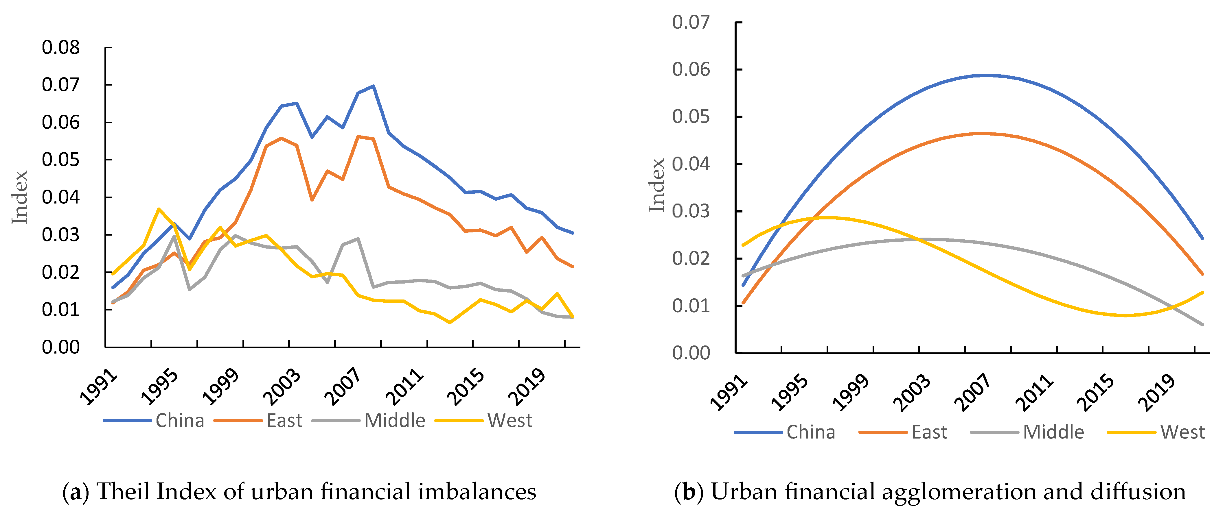
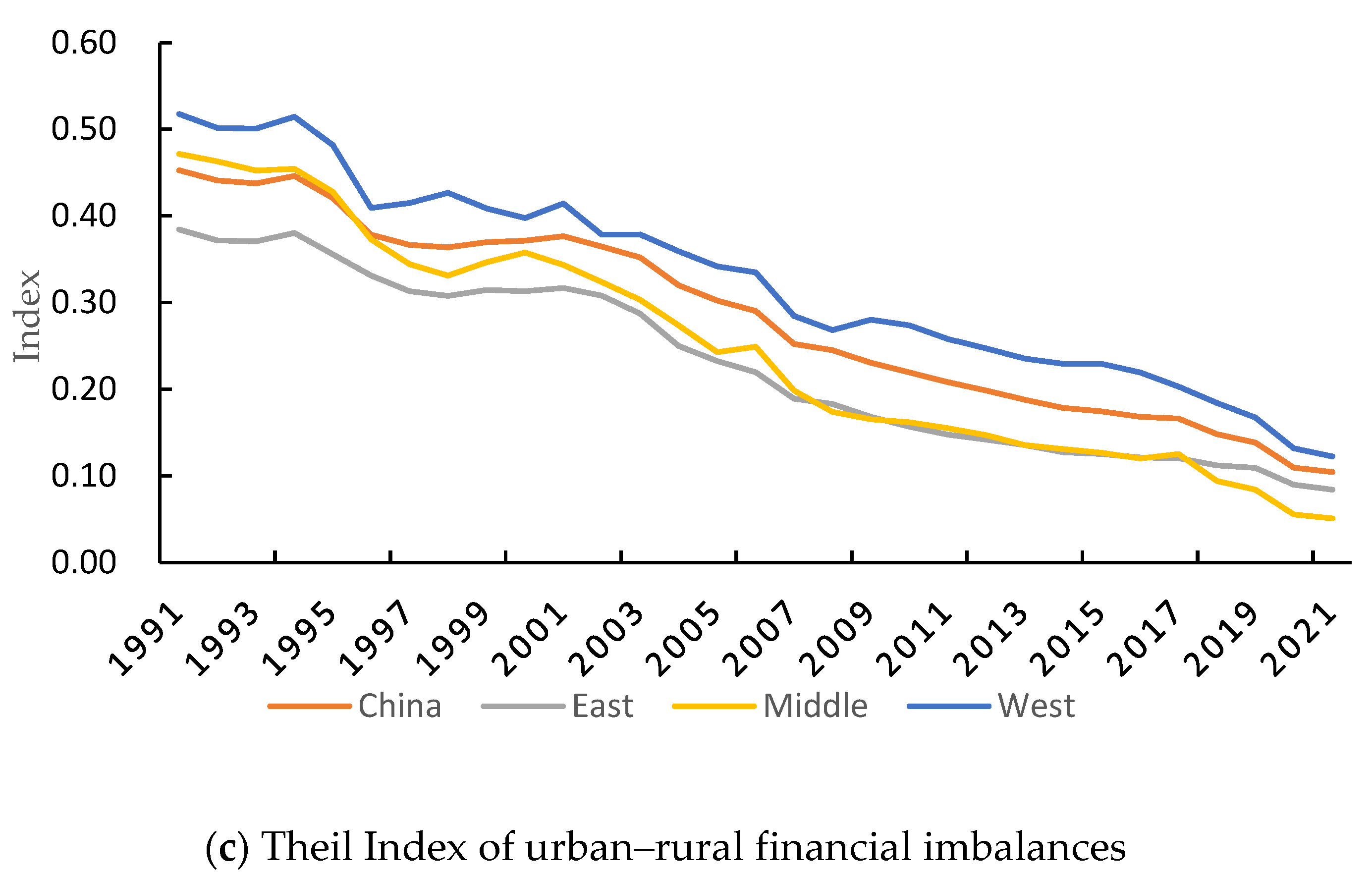
Figure 2a shows the Theil index of urban financial imbalances from 1991 to 2019, calculated according to Equation (2). We can see that urban financial differences in China and the eastern region showed an upward trend before 2003, fluctuated slightly, and then continued to decline. The Theil indexes of urban financial differences in the central and western regions were far lower than that in the eastern region. Figure 2b is the quadratic or cubic curve fitted according to the Theil index. The fitting curves for China and the eastern region showed inverted “U” shapes, indicating an obvious financial agglomeration and diffusion process in the urban areas. The inverted “U” shape of the central region was weak, and the curve of the western region was waved. Figure 2c shows the inter-group difference in urban–rural financial imbalance calculated according to Equation (3), which describes the spatial-temporal evolution of urban–rural financial inequality in China and the three regions. It can be seen that the urban–rural financial imbalance declined continuously. The curve of the western region with the scarcest financial resources was the highest, while that of the eastern part with the most abundant financial resources was the lowest. According to Figure 2a, the Theil index of China increased gradually from 1991 to 2003 and reached a peak of 0.0651. Therefore, we define this interval as the urban financial agglomeration period, and the urban financial diffusion period starting in 20041.
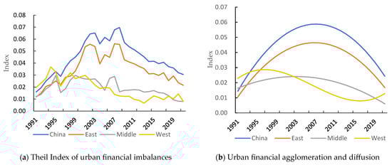
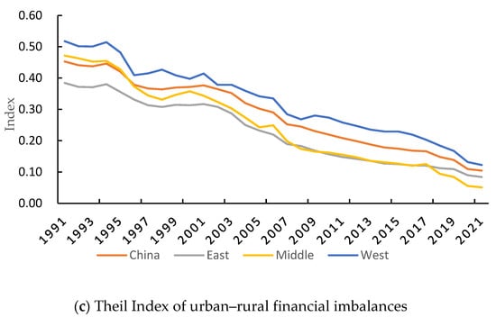
Figure 2.
Space and temporal evolution of urban–rural financial imbalances in China from 1991 to 2019. Note: The eastern region includes Beijing, Tianjin, Hebei, Liaoning, Shanghai, Jiangsu, Zhejiang, Fujian, Shandong, Guangdong, and Hainan. The central region includes Shanxi, Jilin, Heilongjiang, Anhui, Jiangxi, Henan, Hubei, and Hunan. The western region includes Inner Mongolia, Guangxi, Chongqing, Sichuan, Guizhou, Yunnan, Tibet, Shaanxi, Gansu, Qinghai, Ningxia, and Xinjiang.
4.2. Spatial Heterogeneity of Urban–Rural Financial Imbalance
The calculation results of the spatial auto-correlation are described in Table A1, which shows that the Moran index of adjacency weight W1 was significantly positive and the highest. We divided urban–rural financial imbalance (lnurd) into four quartile intervals from low to high, as shown in Figure 3. From 1991 to 2019, the ranges of the first quartile intervals continuously declined. The second and the third quartile interval ranges also tend to be narrow. However, the range of the fourth quartile has not narrowed significantly from 1991 to 2011, which shows that provinces with high urban–rural financial imbalance are dispersed and impede the convergence of urban–rural financial inequality.
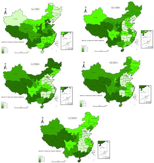
Figure 3.
Quartiles of urban–rural financial imbalances.
The agglomeration characteristics of provinces with a low urban–rural financial imbalance in the eastern regions have been gradually apparent since 1998. Li and Zhang (2017) calculated that Beijing and Shanghai’s comprehensive financial radiation radius is 350–400 km [50]. The two financial centers drove their adjacent provinces to a lower quartile interval from 1991 to 2004; these provinces include Hebei, Shandong, Zhejiang, and Jiangsu, and they all dropped into the first quartile interval in 2004. Financial radiation from financial centers in the eastern regions also extended to the central region. Urban–rural financial imbalance in some provinces of the central areas also decreased from 1991 to 2004. Henan dropped from the third to the first or second quartile interval. Shanxi and Jiangxi dropped from the second to the first quartile interval. Anhui fell step by step from the fourth to the second quartile interval.
Due to the massive outflow of financial resources, a high area of financial exclusion has formed in the western region. Provinces with high financial exclusion, such as Qinghai, Tibet, Yunnan, and Guizhou [51], were always in the third and fourth quartile interval and constantly increased the urban–rural financial imbalance of surrounding provinces. An aggregation of provinces with high urban–rural financial imbalance has appeared since 1998. In 2011, all the western provinces except for Ningxia were concentrated in the third or fourth quartile interval. Financial inclusion levels in rural areas of Guangxi and Guizhou were low [52], and thus these two provinces become stuck in the third and fourth quartile interval in most of the sample years. The influence of high financial exclusion was weakened in 2019, significantly reducing urban–rural financial imbalance in the western provinces. Shaanxi and Guizhou dropped from the fourth to the third quartile interval. Inner Mongolia and Sichuan dropped from the third to the second quartile interval. The spatial dependence and spatial heterogeneity of urban–rural financial imbalance align with the description of hypothesis 1.
4.3. Spatial Spillovers and Convergence of Urban–Rural Financial Imbalances
4.3.1. Spatial Convergence of the Whole Period
Table 2 describes the absolute convergence of urban–rural financial imbalance in China and three regions during the whole period when we take the most significant weight W1 as the spatial weight. As shown in Table 2, urban–rural financial imbalances in China’s eastern and central regions have absolute β convergence characteristics, while the β coefficient in the western part is insignificant. Spatial coefficients ρ and λ in all models are significantly positive, indicating that urban–rural financial imbalances have significant positive spillover effects.
Table 2.
Absolute spatial β convergence of urban–rural financial imbalances (1991–2021).
4.3.2. Spatial Spillovers and Convergence during Urban Financial Agglomeration Period
The results of conditional convergence under spatial weight W1 are shown in Table 3 and Table 4. During the agglomeration period, urban–rural financial imbalances in China and the eastern region showed significant spatial spillovers and convergence. The β coefficients are significantly negative in columns (3) to (4) of Table 3. The spatial coefficients ρ and λ are both significantly positive in columns (3) to (4). During this period, reforms of the rural financial system had started. A trinity financial system featuring cooperative, commercial, and policy-based finance has been gradually established and improved. Initially, urban finance mainly radiated rural finance through the scale expansion of financial services and institutions. Financial radiation spillover had significantly promoted the convergence of urban–rural financial imbalance in eastern China. As mentioned above, financial centers such as Beijing and Shanghai can reduce urban–rural financial inequalities of their peripheral areas through financial radiation. We can see in Figure 3a-c that both Hebei and Shandong dropped from the third or fourth quartile to the first from 1991 to 2004. Jiangsu and Zhejiang were similar, dropping from the third or second quartile to the first. Therefore, peripheral areas can catch up with core regions in the “learning by doing” process, contributing to the convergence of provincial urban–rural financial imbalance in the eastern areas. The convergent characteristics of urban–rural financial imbalance in the eastern regions during the agglomeration period are consistent with the description in hypothesis 2.
Table 3.
Conditional spatial β convergence of urban–rural financial imbalances during urban financial agglomeration period (1991–2003).
Table 4.
Conditional spatial β convergence of urban–rural financial imbalances during urban financial diffusion period (2004–2021).
As shown in Table 3, columns (5) to (6), the coefficients of β are significant in the central region, but the spatial coefficients are not significant. This indicates that spatial spillover effects among the central provinces were not strong. The decrease in urban–rural financial imbalance in the central regions was mainly driven by spatial spillovers of the adjacent provinces in the eastern areas. As we can see from Figure 3a-b, the central provinces such as Shanxi, Henan, Anhui, and Jiangxi, dropped into a lower quartile interval from 1991 to 1998. These characteristics also promote the convergence of urban–rural financial imbalance in China. As we can see in columns (1) to (2) of Table 3, coefficients ρ and λ were significantly positive, and coefficient β was significantly negative.
As to the western region, financial exclusion spillovers hindered the convergence of urban–rural financial imbalance. We can see from Table 3 that coefficients ρ and λ in columns (7) to (8) were significantly positive, while coefficient β was not significant. As seen in Figure 3b,c, urban–rural financial imbalance in the high financial exclusion provinces, such as Qinghai, Tibet, Yunnan, and Guizhou [51], were always in the third and fourth quartile intervals, which constantly raised the urban–rural financial imbalance of surrounding provinces through exclusion spillovers. Consequently, high financial exclusion induced an agglomeration of provinces with high urban–rural financial imbalance, which prevented convergence in the western region. The convergent characteristics of urban–rural financial inequality in the western areas during the agglomeration period are consistent with the description in hypothesis 2.
The spillover effect based on financial radiation and financial exclusion decreased with geographical distance. To test the geographical boundary of spatial spillover effects, we used 50 rounds of consecutive regression according to the spatial SEM model of Equations (9) and (10), starting from the shortest distance of 115.46 km, with 50 km adopted as the progressive distance until 2565.46 km was reached. It was found that the significance of the spatial spillover coefficients in the first 46 regressions was 1%, and then decreased beyond this distance. Therefore, the results within 2365.46 km were analyzed. The spatial coefficients and geographical distances are shown in Figure 4 and are divided into four distance intervals. The first interval was within 365.46 km, where the spatial spillover coefficients were from 0.3427 to 0.3623. The distances between Beijing, Tianjin, and Hebei and between Shanghai, Jiangsu, and Zhejiang are in this interval, showing strong spillover effects based on financial radiation. The distance of this interval is mostly consistent with the comprehensive financial radiation radius of Beijing and Shanghai, which are around 350–400 km [50]. The second interval was from 415.46 km to 615.46 km. This distance is beyond the strongest financial radiation radium of financial cores such as Beijing and Shanghai, so the spatial spillover coefficients dropped rapidly from 0.3270 to 0.1871. The third interval was 665.46–865.46 km, in which spatial spillover effects rebound. The distances between high financial exclusion provinces, such as Yunnan and Guizhou, Yunnan and Guangxi, are within this range. Positive spillovers of financial exclusion increased spatial spillover coefficients from 0.2445 to 0.4003. The fourth interval was 915.46–2365.46 km, and the spatial coefficients showed a fluctuating downward trend. According to the above analysis, positive spatial spillover effects of urban–rural financial imbalance are based on financial radiation spillovers in financially abundant areas and financial exclusion spillovers in financially scarce areas with obvious geographical boundaries, consistent with the description in hypothesis 1.
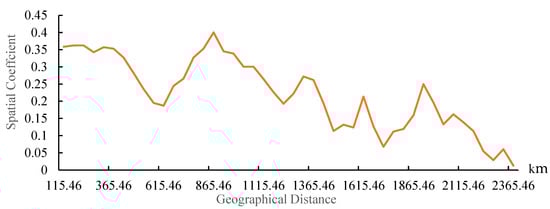
Figure 4.
Relationship between spatial coefficients and geographical distance. Note: The spatial spillover effects are significant in the financial agglomeration stage (1991–2003), so we choose this period for analysis.
4.3.3. Spatial Spillovers and Convergence during Urban Financial Diffusion Period
The spatial spillover effect in the eastern regions during the financial diffusion period was weaker. The convergence was insignificant, as shown in columns (3) and (4) of Table 4. The spatial coefficient λ was insignificant, and the significance of ρ also decreased compared with the values in Table 3. As mentioned, two reasons exist for the decline in the convergence of urban–rural financial inequality in the eastern area. First, the reduction in urban–rural financial disequilibrium was moderated by weak financial radiation. A series of changes occurred in the rural financial market environment. The entry conditions for rural banking institutions have been relaxed since 2006, allowing domestic and foreign banking capital, industrial capital, and private capital to invest in rural areas. New types of rural financial institutions have gradually emerged. New mortgage guarantee models, agricultural futures options, and rural supply chain finance were continuously introduced. Internet and mobile finance development in rural areas have made financial services more interconnected and convenient. The continuous introduction of financial innovations have transformed rural financial demands. The financial radiation from urban to rural areas needs to shift away from promoting the expansion of financial scale to improving the quality of rural finance. Otherwise, the ineffectiveness of financial radiation will hinder the decline of urban–rural financial imbalance in the eastern areas.
Second, the weakening of spatial linkages also slows the convergence under geographical weight. The mobility of financial resources in the Yangtze River Delta Economic Circle and Bohai Rim Economic Circle of the eastern region during the period of financial diffusion has weakened significantly [49], which contributes to the weakening of the spatial spillovers at the geographical level. Accordingly, the intensity of radiation spillovers decreased, which diverges from the trends of urban–rural financial imbalance in the eastern regions. As shown by Figure 3c–e, Shanghai’s urban–rural financial imbalance has increased since 2004 and gradually into the fourth quartile in 2019. Jiangsu moved from the first to the second quartile interval in 2011, and Zhejiang moved from the first to the second quartile in 2019, chasing after Shanghai. Beijing, Tianjin, Hebei, and Shandong stayed in the first quantile in 2011 and 2019. Guangdong has been in the fourth quartile since 2004, affected by its neighbor Guangxi, which has a high level of financial exclusion [51]. We can see from the above analysis that urban–rural financial imbalance diverged in the financial diffusion stage, which prevent their convergence, as described by hypothesis 3.
At this stage, the backflow of financial resources from the eastern region to the western region reduced financial exclusion and improved financial radiation from urban to rural areas. Accordingly, urban–rural financial imbalances in the western provinces decreased. Coefficients ρ and λ in columns (7) to (8) of Table 4 were not significant, indicating that spillover effects of financial exclusion were weakened. As shown by columns (7) to (8) of Table 4, the β coefficients were significantly negative. We can infer from the above analysis that the improved financial radiation from urban to rural areas and weakened exclusion spillovers can enhance the convergence in financially scarce areas, according with hypothesis 3.
In terms of the convergence mechanism, the coefficients of mpkur in Table 3 and Table 4 showed negative relationships with gur in most models, suggesting that marginal returns of capital do not drive the convergence of urban–rural financial imbalances. However, convergence can be achieved in an interactive catch-up process between regions when spatial spillover is considered [18]. The empirical results of this paper showed that the spatial interactions between regions has a significant impact on the convergence of urban–rural financial inequality during the financial agglomeration and financial diffusion phases.
The coefficients of rgov were significantly positive in most models during the financial diffusion stage, as shown in Table 4, which follows our expectation. The coefficients of Market were not significant in most models. From Table 3 and Table 4, rfdi was significantly positive in most models at the financial agglomeration stage, which is consistent with our expectations. Traffic was significantly positive in both the overall Chinese sample and the eastern sample at the financial diffusion stage, which is consistent with our expectations. This indicates that areas with better traffic conditions are more attractive to financial resources in urban areas, thus increasing gur. The volatility in most models was negatively related to gur, which follows our expectations, but was only significant in columns (1), (5) and (6) of Table 3.
4.3.4. Robustness Test
Robustness tests were carried out from two aspects in this paper. First, the spatial weight was changed. We used the product of adjacent weight and economic weight as the spatial weight W3, and the results are shown in Table A2. We can see that urban–rural financial imbalances in the eastern region converged significantly in the agglomeration period. In contrast, those in the western region converged significantly in the diffusion period. Moreover, the positive spillover effects in the eastern and western regions were significant during the agglomeration period while obviously decreasing during the diffusion period. The aforementioned spatial spillover effects and spatial convergence characteristics were consistent with those under the adjacent weight, indicating that the empirical conclusions of spatial convergence were robust. Second, considering that the impact of the financial crisis in 2008 may affect the urban financial system and its convergence trend, we divided the diffusion periods into two stages, before and after the crisis, for comparative analysis. As shown in Table A3, the coefficient of volatility in the three regions was insignificant before and after the crisis, indicating that the output volatility caused by the financial crisis had no apparent impact on urban–rural financial imbalance and the convergence mechanism of urban–rural financial inequality was robust.
4.4. Further Analysis
As mentioned above, the positive spillovers under the adjacent weight weakened during the financial diffusion period, reducing the linkage between urban and rural financial imbalances. New spillover channels need to be stimulated to sustain the convergence of the urban–rural financial imbalance. At this stage, with the rise of internet finance and financial technology, spillovers in the dimension of technology and information start to play an important role. Therefore, we further analyzed the spatial spillover and convergence of urban–rural financial imbalances under the spatial weights of technology (Wt) and internet distance (Wi)2. The results are shown in Table 5 and Table 6.
Table 5.
Convergence for urban–rural financial imbalances under technology weights (2006–2021).
Table 6.
Convergence for urban–rural financial imbalances under internet weights (2006–2021).
The positive spillover effects and the convergent trends were more substantial under the technology and internet weights than the geography weights in the middle and western regions. As shown by columns (5)–(8) of Table 5 and Table 6, both ρ and λ were significantly positive. β was more significantly negative compared with columns (5) to (8) in Table 4. The results show that more spatially penetrating channels were motivated through the exchange of information and the diffusion of technology, driving the convergence of urban–rural financial imbalances in the information and technology dimensions. However, the spatial coefficients ρ and λ of the eastern region were not significant, making it hard to drive spatial convergence. As shown by columns (3) and (4) of Table 5 and Table 6, the β coefficient became negative, but not significant. We can infer that the spatial interactions within the internet and information dimensions have broken through geographical limitations, enabling the central and western regions to take advantage of backwardness and generate more obvious significant spatial spillovers, thus promoting the spatial convergence of urban–urban financial disequilibrium in these areas.
5. Discussion
The existing studies have explored the convergence of urban–rural financial disequilibrium without spillovers. In contrast, our study examined the spatial spillover effects of provincial urban–rural financial imbalances, their heterogeneous characteristics, and their important role in spatial convergence. The possible contribution of this study is that we constructed a framework to analyze the spatial convergence of urban–rural financial imbalances under spatial spillovers. It is based on the analytical paradigm of spatial process, spatial action, and spatial convergence from the perspective of financial geography. We used this framework to explain heterogeneous spatial spillovers formed during the spatial process of urban financial agglomeration and diffusion, and their impact on the convergent mechanism. Further, through the spatial econometric models, we re-examined the spatial convergence of urban–rural financial imbalances in China from 1991 to 2021.
Our results verified the proposed hypothesis that spatial spillovers exist in provincial urban–rural financial imbalances and influence their spatial convergence. First, urban–rural financial imbalances showed significant spillover effects and heterogeneous characteristics. Spillovers based on financial radiation and exclusion were apparent during financial agglomeration, and decreased with geographical distance. Radiation spillovers in financially abundant areas promoted the concentration of provinces with low urban–rural financial imbalance. On the other hand, exclusion spillovers in financially scarce regions contributed to the concentration of provinces with high urban–rural financial imbalances. Second, spatial spillovers had an essential impact on the convergence of provincial urban–rural financial imbalance. During the financial agglomeration period, radiation spillovers from financial centers in the eastern region drove peripheral provinces to reduce their urban–rural financial inequality, contributing to the convergence in financially abundant areas. On the other hand, some provinces in the northwest and southwest regions were locked into the accumulation of high urban–rural financial imbalances because of financial exclusion spillovers, hindering the convergence in financially scarce areas. During the financial diffusion period, the convergence of urban–rural financial inequality in the eastern region weakened because of the decreased intensity of radiation spillovers. Meanwhile, convergence in the western area improved with the decline of exclusion spillovers.
This study was subject to some limitations. Firstly, it was mainly limited to the provincial level due to data availability. Municipal data can be considered to compare urban–rural financial imbalances of different urban agglomerations and the impact of spillovers on their convergence. Secondly, the spatial correlation network should be further explored. With the increased complexity of urban spatial connections, the linkage structure of urban–rural financial imbalances gradually developed into a complex network. Subsequent research can use social network analysis to study their network characteristics and more accurately investigate the spatial role of urban–rural financial imbalance in different regions. Thirdly, this study focused on urban–rural differences in traditional finance, and differences in digital finance require more attention in the future, especially the impact of technology and information spillovers on urban–rural digital financial differences. They are not constrained by geographic distances and can better reflect the spatial spillovers of digital finance.
According to our research, it is necessary to establish a concept of spatial integration to promote the convergence of urban–rural financial imbalances based on promoting spatial synergy. Policy recommendations are as follows. Firstly, improve urban financial radiation by meeting the financial demands of rural areas in different regions. Ineffective financial radiation will lead to excessive concentration of financial resources in cities and inhibit the convergence of urban–rural financial disequilibrium. Therefore, urban financial radiation should be optimized regarding radiation sources and radiation channels according to changes in rural finance. Secondly, it is necessary to reasonably use spatial spillover effects to promote the convergence of urban–rural financial imbalance. Inclusive finance should be promoted according to different spatial spillover effects among regions, strengthening financial radiation spillover and suppressing financial exclusion spillover. Thirdly, new spatial spillover channels should be activated according to the changes in the spatial interaction mode of urban–rural financial disequilibrium. Interaction channels such as via the transfer of information and the diffusion of knowledge, should be explored when spillover based on geographical distance is weak. The eastern region should expand networked and information-based spillover channels, improving the spatial dissemination of financial technology and encouraging the financial interaction in the information and technology dimensions. The central and western regions should continue enhancing urban–rural information construction and the digital upgrade of rural financial institutions to further improve the convergence of urban–rural financial disequilibrium for information and technology adjacent regions.
6. Conclusions
This study aimed to investigate the convergent mechanism of urban–rural financial disequilibrium under spatial spillovers. From the perspective of financial geography, we explained the logical framework of spatial process, spatial interaction, and spatial convergence. Then, we conducted an empirical study on the spatial convergence of urban–rural financial imbalances in China from 1991 to 2021 under spatial spillovers. We found that inter-provincial urban–rural financial imbalances have obvious spatial spillovers and influence their spatial convergence. Financial radiation and exclusion spillovers based on geographical distance have important impacts on the convergence at the stage of urban financial agglomeration. When such spillovers weaken during urban financial diffusion, spatial spillovers at the level of technology and information, which are less constrained by geographic distances, begin to play a role in spatial convergence. Following the changes in the spatial interaction modes, it is necessary to activate different spatial spillover channels. In summary, the spatial spillover effect should be properly utilized to weaken urban–rural financial imbalances for the harmonious development of urban–rural finance.
Author Contributions
Conceptualization, Y.Y.; methodology, Y.Y.; software, H.R.; validation, P.G.; formal analysis, Y.Y.; resources, H.R.; data curation, Y.L.; writing—original draft, Y.Y.; writing—review and editing, Y.L.; visualization, P.G. All authors have read and agreed to the published version of the manuscript.
Funding
This research was funded by the Shaanxi Social Science Fund (No. 2020D037).
Institutional Review Board Statement
Not applicable.
Informed Consent Statement
Not applicable.
Data Availability Statement
The data presented in this study are available on request from the corresponding author.
Conflicts of Interest
The authors declare no conflict of interest.
Appendix A
Table A1.
Moran’s I Index of urban–rural financial imbalances in China.
Table A2.
Conditional spatial β convergence of urban–rural financial imbalances (W3 as Spatial Weight).
Table A3.
Conditional spatial β convergence of urban–rural financial imbalances during urban financial diffusion period.
Notes
| 1 | Yu et al., (2017) showed that China’s regional financial diffusion began in 2005 [49]. However, urban financial diffusion would be earlier than that of the regions. Therefore, based on the Theil index in this paper, we defined urban financial diffusion as starting from 2004. |
| 2 | Wt and Wi are the reciprocal of the technology distance and information distance of the two provinces, respectively. Technology distance is the difference in the number of patent audits per capita. Information distance is the difference in the percentage of people with internet access. By comparing the different time periods, it was found that the spillovers of these two channels were more significant after 2006, so the sample interval was set as 2006–2021. |
References
- Bai, Q.X. Introduction to Financial Sustainability Research; China Financial Publishing House: Beijing, China, 2001. [Google Scholar]
- Feng, Y.D.; Zou, L.H.; Yuan, H.X.; Dai, L. The spatial spillover effects and impact paths of financial agglomeration on green development: Evidence from 285 prefecture-level cities in China. J. Clean. Prod. 2022, 340, 130816. [Google Scholar] [CrossRef]
- Yuan, H.X.; Zhang, T.S.; Feng, Y.D.; Liu, Y.B.; Ye, X.Y. Does financial agglomeration promote the green development in China? A spatial spillover perspective. J. Clean. Prod. 2019, 237, 117808. [Google Scholar] [CrossRef]
- Hu, S.H.; Guo, Y.L.; Yang, T. Information Asymmetry, Financial Connectivity and Credit Allocation: Empirical Research Based on Farmers Survey Data. J. Agrotech. Econ. 2016, 250, 81–91. [Google Scholar]
- Zhou, H.W.; Tian, L. An Optimization of the Credit Technology in Rural Financial Institutions: Based on a Survey of Information Asymmetry and Transaction Costs. Issues Agric. Econ. 2019, 473, 58–64. [Google Scholar]
- Liu, C.K. Government Urban Preference, Network Information and Basic Public Services Equalization between Urban and Rural Area. Financ. Tr. Res. 2013, 24, 78–86. [Google Scholar]
- Huang, K.; Zhu, Y. Is Bank Credit Discrimination the Result of Government Intervention: Evidence from the Reform Process. Contemp. Financ. Econ. 2020, 424, 50–63. [Google Scholar]
- Zhou, Z.; Wu, Z.J.; Kong, X.Z. Mechanisms, Scale and Trends of Net Flow of Rural Capital in China: 1978–2012. J. Manag. World 2015, 256, 63–74. [Google Scholar]
- Chen, F. On the Flow and Integration of Urban-Rural Financial Capital in China. Shanghai J. Econ. 2023, 412, 85–93. [Google Scholar]
- Chen, J. The Political Economy of the Development of Rural-Urban Financial Relations in China. Jianghan Trib. 2018, 486, 31–37. [Google Scholar]
- Jiang, Y.; Xie, J.Z. The Threshold Effect of Urban-rural Financial Development: Based on the View of Interaction in Economic Transformation. J. Cent. Univ. Financ. Econ. 2015, 334, 37–45. [Google Scholar]
- Lu, Z.Y. The Measurement and Trend of Unbalanced Development of Regional Urban and Rural Finance in China—Based on the Perspective of Urban and Rural Financial Development at the Regional Level. Inq. Econ. Issues 2013, 369, 86–94. [Google Scholar]
- Wang, T. Estimation and Analysis on Discrepancies of Financial Resource Allocation in China’s Urban and Rural Areas. Econ. Probl. 2011, 384, 95–98. [Google Scholar]
- Li, S.; Lu, Z.Y. Convergence Analysis of Unbalanced Development of China’s Urban and Rural Finance. Chin. Rural Econ. 2014, 351, 27–35+47. [Google Scholar]
- Clark, G.L. Money flows like mercury: The geography of global finance. Geogr. Ann. B 2005, 87, 99–112. [Google Scholar] [CrossRef]
- Li, W.M.; Wang, X.Y. The role of Beijing’s securities services in Beijing-Tianjin-Hebei financial integration: A financial geography perspective. Cities 2020, 100, 102673. [Google Scholar] [CrossRef]
- Ding, X.; Zhou, Y. The tug-of-war for Financial Development: An Analysis of Asymmetric Spatial Spillovers from Financial Agglomeration and Financial Exclusion. Res. Econ. Manag. 2022, 43, 87–109. [Google Scholar]
- Chen, F.L.; Wang, M.C.; Xu, K.N. The Evolution Trend of China’s Coordinated Regional Development: A Spatial Convergence Analysis. Financ. Trade Econ. 2018, 39, 128–143. [Google Scholar]
- Anselin, L. Lagrange Multiplier Test Diagnostics for Spatial Dependence and Spatial Heterogeneity. Geogr. Anal. 1988, 20, 1–17. [Google Scholar] [CrossRef]
- Ying, L.G. Understanding China’s recent growth experience: A spatial econometric perspective. Ann. Reg. Sci. 2003, 37, 613–628. [Google Scholar] [CrossRef]
- Rey, S.J.; Dev, B. σ-convergence in the presence of spatial effects. Pap. Reg. Sci. 2006, 85, 217–234. [Google Scholar] [CrossRef]
- Liu, H.J.; Jia, W.X. Convergence test and coordinated development of regional economic growth in China under different spatial network association scenarios. Nankai Econ. Res. 2019, 207, 104–124. [Google Scholar]
- Shi, B.; Ren, B.P. Strategic competition, spatial effects and convergence of economic growth in China. Dyn. Econ. 2019, 696, 47–62. [Google Scholar]
- Qin, C.L.; Liu, Y.X.; Li, C. Spatial Spillovers and the Convergence of Regional Economic Growth: A Case Study Based on the Yangtze River Delta. Soc. Sci. China 2013, 34, 159–173. [Google Scholar]
- Wang, L.W.; Kong, R. Measurement of the level of high-quality development of rural finance, regional differences and spatial convergence analysis. Stat. Decis. 2023, 39, 135–140. [Google Scholar]
- Fujita, M.; Krugman, P.; Mori, T. On the evolution of hierarchical urban systems. Eur. Econ. Rev. 1999, 43, 209–251. [Google Scholar] [CrossRef]
- Moroni, S.; Rauws, W.; Cozzolino, S. Forms of self-organization: Urban complexity and planning implications. Environ. Plan. B Urban Anal. City Sci. 2020, 47, 220–234. [Google Scholar] [CrossRef]
- Loginova, J.; Sigler, T.; Searle, G.; O’Connor, K. The distribution of national urban hierarchies of connectivity within global city networks. Glob. Netw. 2022, 22, 274–291. [Google Scholar] [CrossRef]
- Partridge, M.D.; Rickman, D.S.; Ali, K.; Olfert, M.R. Do new economic geography agglomeration shadows underlie current population dynamics across the urban hierarchy? Pap. Reg. Sci. 2009, 88, 445–466. [Google Scholar] [CrossRef]
- Zhu, J.M.; Zhu, M.W.; Xiao, Y. Urbanization for rural development: Spatial paradigm shifts toward inclusive urban-rural integrated development in China. J. Rural Stud. 2019, 71, 94–103. [Google Scholar] [CrossRef]
- He, Y.H.; Zhou, G.H.; Tang, C.L.; Fan, S.G.; Guo, X.S. The spatial organization pattern of urban-rural integration in urban agglomerations in China: An agglomeration-diffusion analysis of the population and firms. Habitat Int. 2019, 87, 54–65. [Google Scholar] [CrossRef]
- Wang, Z.Z.; Huang, X.S. On the spatial logic of urban-rural integration and development. Theor. Mon. 2023, 494, 112–122. [Google Scholar]
- Risto, L. Financial Geography: A Banker’s View; The Commercial Press: Beijing, China, 2001. [Google Scholar]
- French, S.; Leyshon, A.; Wainwright, T. Financializing Space, Spacing Financialization. Prog. Hum. Geogr. 2011, 35, 798–819. [Google Scholar] [CrossRef]
- Sun, Z.J.; Li, X. An Empirical Analysis on Spatial Spillover Effect and Convergence of Cultural Industries in China. Chin. Soft. Sci. 2015, 296, 173–183. [Google Scholar]
- Sarma, M.; Pais, J. Financial Inclusion and Development. J. Int. Dev. 2011, 23, 613–628. [Google Scholar] [CrossRef]
- Zhang, G.J.; Yao, Y.Y.; Zhou, C.S. Spatial Characteristics and Spatial Effect of Chinese Provincial Financial Exclusion. Trop. Geogr. 2018, 38, 176–183. [Google Scholar]
- Han, J.J.; Guo, X.B. Research context and new progress of diffusion echo effect. Econ. Dyn. 2014, 636, 117–125. [Google Scholar]
- Lin, G.P.; Long, Z.H.; Wu, M. A Spatial Investigation of σ-convergence in China. J. Quant. Technol. Econom. 2006, 4, 14–21+69. [Google Scholar]
- Barro, R.J.; Sala-I-Martin, X. Barrow and Martin Convergence. J. Polit. Econ. 1992, 100, 223–251. [Google Scholar] [CrossRef]
- Gao, F.; Li, T. Is there “Lucas Paradox” in urban-rural capital flow in China? Economist 2016, 207, 75–86. [Google Scholar]
- Zhang, J.; Jin, Y. Analysis on Relationship of Deepening Financial Intermediation and Economic Growth in China. Econ. Res. J. 2005, 11, 34–45. [Google Scholar]
- Zhou, L. Four major problems of rural financial market and their evolutionary logic. Financ. Trade Econ. 2007, 303, 56–63. [Google Scholar]
- Liao, C.W.; Zhang, Z.D. Local Government Intervention and Total Factor Productivity: From the Perspective of Resource Mismatch. Econ. Surv. 2023, 40, 3–12. [Google Scholar]
- Shi, B.; Shen, K.R. Government Intervention, Economic Agglomeration and Energy Efficiency. J. Manag. World 2013, 241, 6–18+187. [Google Scholar]
- Yan, T.F.; Yuan, A.N.; Xu, X.C. Internet Finance, Government Intervention and the Quality of Economic Growth—An Empirical Test Based on Panel Threshold Regression Models. Public Financ. Res. 2019, 439, 47–61. [Google Scholar]
- Zhao, Q.Y.; Li, C.M.; Hu, Q.Y. Local Government Intervention and Labor Income Shares: A Perspective Based on the Tax Sharing System. Econ. Theory Bus. Manag. 2017, 324, 36–46. [Google Scholar]
- Lu, Q.Q.; Xu, G.J.; Xu, K. Urbanization, Business Cycleand Regional Income Distribution Disparity: An Analysis Based on Panel Threshold Model. Econ. Probl. 2020, 486, 25–32. [Google Scholar]
- Yu, Y.; Su, H.K.; Li, Y. The Evolution Path and Mechanism of Regional Financial Difference. Chin. Ind. Econ. 2017, 349, 74–93. [Google Scholar]
- Li, K.F.; Zhang, Z. Analysis of Financial Efficiency of Financial Radiation in China’s Regional Financial Centers. Stat. Decis. 2017, 470, 171–173. [Google Scholar]
- Li, C.X.; Jia, J.R. Research on the Extent of Financial Exclusion in China-Construction and Measurement Based on Financial Exclusion Index. Mod. Econ. Sci. 2012, 34, 9–15. [Google Scholar]
- Gao, P.X.; Wang, X.H. Regional Differences and Impact Factors of Rural Financial Exclusion in China-Empirical analysis based on interprovincial data. J. Agrotech. Econ. 2011, 192, 93–102. [Google Scholar]
Disclaimer/Publisher’s Note: The statements, opinions and data contained in all publications are solely those of the individual author(s) and contributor(s) and not of MDPI and/or the editor(s). MDPI and/or the editor(s) disclaim responsibility for any injury to people or property resulting from any ideas, methods, instructions or products referred to in the content. |
© 2023 by the authors. Licensee MDPI, Basel, Switzerland. This article is an open access article distributed under the terms and conditions of the Creative Commons Attribution (CC BY) license (https://creativecommons.org/licenses/by/4.0/).