Identification of Urban Clusters Based on Multisource Data—An Example of Three Major Urban Agglomerations in China

Abstract

Accurately identifying the boundary of urban clusters is a crucial aspect of studying the development of urban agglomerations. This process is essential for comprehending and optimizing smart and compact urban development. Existing studies often rely on a single category of data, which can result in coarse identification boundaries, insufficient detail accuracy, and slight discrepancies between the coverage and the actual conditions. To accurately identify the extent of urban clusters, this study proposes and compares the results of three methods for identifying dense urban areas of three major agglomerations in China: Beijing–Tianjin–Hebei, the Yangtze River Delta, and the Guangdong–Hong Kong–Macao Greater Bay Area. The study then integrates the results of these methods to obtain a more effective identification approach. The social economic method involved extracting a density threshold based on the fused nuclear density of socio-economic vitality data, including population, GDP, and POI, while the remote sensing method evaluated feature indices based on remote sensing images, including the density index, continuity index, gradient index, and development index. The traffic network method utilizes land transportation networks and travelling speeds to identify the minimum cost path and delineate the boundary by 20–30 min isochronous circles. The results obtained from the three methods were combined, and hotspots were identified using GIS overlay analysis and spatial autocorrelation analysis. This method integrates the multi-layered information from the previous three methods, which more comprehensively reflects the characteristics and morphology of urban clusters. Finally, the accuracy of each identification result is verified and compared. The results reveal that the average overall accuracy (OA) of the three areas delineated by the first three methods are 57.49%, 30.88%, and 33.74%, respectively. Furthermore, the average Kappa coefficients of these areas are 0.4795, 0.2609, and 0.2770, respectively. After performing data fusion, the resulting average overall accuracy (OA) was 85.34%, and the average Kappa coefficient was 0.7394. These findings suggest that the data fusion method can effectively delineate dense urban areas with greater accuracy than the previous three methods. Additionally, this method can accurately reflect the scope of urban clusters by depicting their overall boundary contour and the distribution of internal details in a more scientific manner. The study proposes a feasible method and path for the identification of urban clusters. It can serve as a starting point for formulating spatial planning policies for urban agglomerations, aiding in precise and scientific control of boundary growth. This can promote the rational allocation of resources and optimization of spatial structure by providing a reliable reference for the optimization of urban agglomeration space and the development of regional spatial policies.

1. Introduction

The new type of urbanization is a powerful driver for promoting high-quality development in China’s economy and society. As the primary form of new-type urbanization and the spatial carrier for coping with the new economic norm, China’s urban agglomerations and metropolitan areas accommodate over 80% of the population and contribute to nearly 90% of the country’s GDP. Urban clusters, in particular, will continue to play a significant role in high-quality development of the new era, given the increasing radiative effect of a group of central cities [1]. Reasonably defining the boundaries of urban clusters is an essential requirement for understanding urban agglomerations, as well as a fundamental condition for implementing regional functional spatial layout and development planning. Urban clusters are currently facing several challenges, including scattered and disorderly spatial layouts, a lack of synergy in regional development, and significant pressure on natural resources and the environment [2]. As a complex urban system, overall coordinated development is essential for the intensive development of urban clusters, with regional level planning being crucial. The regional space consists of urban nodes, supporting networks, and environmental substrates that interact as structural elements. Intensive development in urban clusters should aim for efficiency instead of blindly pursuing speed. However, it is important to acknowledge the general shortage of construction land resources in urban clusters, particularly in central cities. Thus, effective ways of expanding space should prioritize maintaining high construction density and a certain urban scale while preserving good environmental quality. Optimizing the structure of urban systems and promoting the coordinated development of large, medium, and small cities is an increasingly important focus of China’s urbanization strategy. To diagnose urban system problems, it is essential to identify the extent of urban clusters and evaluate the degree of urban development using quantitative tools [3].

The urban cluster is a particular form of regional spatial organization that has emerged at a certain stage of social and economic development in China. Due to the degree of economic development, the growth level of the town, the interactions between towns, the extent of opening up, and the infrastructure level being much greater than those in other areas, urban clusters have unique characteristics [4]. After P. Geddes put forward the concept of conurbation [5], scholars have studied the definition, scoping, formation mechanisms, and operation modes of urban clusters [6,7]. Related concepts, such as the megalopolis, world cities, the urban complex, the urban field, the extended metropolitan region, the mega-urban region, etc., have been developed [8,9,10]. The understanding of the essential concept of urban clusters is deepening, and there is agreement on the evolutionary law of urban agglomeration of “built-up area—central city—metropolitan area—joint metropolitan area—urban contiguous area—metropolitan contiguous area” [11]. In particular, an urban cluster generally refers to a densely populated urban area with multiple large- and medium-sized cities at its core, closely linked between cities and regions, with a high level of urbanization and a continuous distribution of cities and towns within a specific territorial area. From the “Sunan model” of rural industrialization to the recent development of “urban–rural integration,” rural development and planning in the Suzhou region serves as a typical example of well-developed urban clusters. Additionally, in the Chengyu urban agglomeration, the national plan has designated three urban clusters: the Chuannan Urban Cluster centered around Luzhou and Yibin, the Nansuiguang Urban Cluster centered around Nanchong, and the Dawan Urban Cluster centered around Wanzhou.

The research on spatial identification of the urban physical extent typically begins with boundary identification for a single city. However, the identification of the physical space of urban agglomerations and urban clusters started relatively late [12]. While the boundaries of cities or urban agglomerations are fixed in terms of administrative divisions, land use is a complex geographical concept that integrates natural and socio-economic characteristics. Consequently, the actual boundaries of urban areas during development are often uncertain [13]. Therefore, it is inappropriate to describe the development of urban clusters out of actual boundaries only based on administration [14]. With the introduction of gravity model [15] and field strength model [16], the methods used to identify actual urban boundaries have developed from qualitative descriptions to mathematical simulations [17,18], becoming a typical paradigm for studying the gradual decay of urban centers and peripheral radiation. The results are not presented by administrative divisions but as clustered patches [19]. In recent years, scholars have taken innovative approaches to identify urban spatial boundaries by exploring the spatial fractal features of the urban form and the cluster degree of the regional road network [20]. Some studies have identified urban clusters based on the agglomeration of elements such as population density [21], POI density [22], and office building area density [23] and have delineated areas that meet certain thresholds as central or dense areas. However, different interpretations of urban clusters have led to diverse perspectives on their range identification, which has limited the applicability of their results in aiding regional planning and management.

With the proliferation of research methods, the erstwhile approach of identifying small-scale metropolitan areas through a top-down approach using solely socio-economic indicators has given way to a more advanced methodology. This entails defining large-scale urban agglomerations and interlocking metropolitan regions based on remote sensing images [24,25]. Compared to traditional methods, remote sensing images provide better spatial features of urban landscapes and infrastructure [26], which can help characterize the range in human activity or the physical distribution pattern of a town [27]. Recent studies have focused on extracting impervious surfaces from satellite images to represent the actual town areas [28,29] due to their higher resolution and lower threshold dependence [30]. However, this method may lead to confusion between impervious surfaces and natural landscapes, such as watersheds, forests, and parks [31]. Luqman et al. combined Landsat data with information on nighttime lighting and travel time distance to accurately delineate the boundaries of the city with both stability and accuracy [32]. However, this method is limited by the high cost of data acquisition, which may restrict the selection of study units. Overall, recent research has shifted from identifying spatial ranges to detecting spatial pattern characteristics within urban agglomerations. The construction of multidimensional feature indices increasingly relies on multi-source data, although the methods of data fusion have not been thoroughly developed [33]. Moreover, increasing attention has been given to the spatial inequality between different areas within urban agglomerations. With the proliferation of research on urban big data, location services based on data analysis have emerged, providing a human-centered perspective for understanding urban space [34]. Initially, research on urban agglomerations defined physical territories based on size and density; however, related studies have since shifted towards defining functional territories based on the degree of city connection. Consequently, there has been a growing focus on flow space and linkage networks in urban research [35].

In summary, despite extensive studies on the range and boundaries of urban agglomerations from various perspectives, several challenges persist. These include imprecise identification boundaries, inadequate attention to detail, and a lack of consistency between coverage and the actual urban situation. The difficulty in achieving a consensus on the identification of urban clusters can be attributed to several factors, such as the ambiguity in the essence of the concept, the formulation of extraction criteria, the selection of the appropriate analysis unit, and the identification method [36,37]. The limitations of this approach are primarily reflected in three key aspects. First, it can be challenging to identify the spatial extent of urban clusters due to their complexity [38]. Traditional demographic and socio-economic data may need to be spatially refined, which can lead to time lags and insufficient resolution, ultimately making it more difficult to determine urban cluster boundaries quickly and accurately [39]. The second limitation pertains specifically to China and concerns the need for more unified identification criteria in urban agglomeration planning studies. Currently, the country lacks a unified national standard for delineating urban agglomerations [40]. Additionally, the spatial extent of these agglomerations has been expanding indiscriminately, driven by larger economic interests and strong political considerations at higher levels of spatial decision-making [41]. The third limitation concerns the degree of fusion of multi-source data, which requires improvement. Many studies only combine different types of data in a complementary manner, overlooking the disparities in spatial properties expressed by each dataset. Furthermore, determining the threshold for extracting boundaries from each type of data is often challenging [42,43]. This study attempts to leverage multi-source data to identify and analyze the spatial features of the urban clusters of the three major urban agglomerations in China, through the utilization of three methods: the social economic method (SEM), the remote sensing method (RSM), and the traffic network method (TNM). Specifically, the study employs a combination of socio-economic data with density threshold curves, remote sensing data with an evaluation system, and transportation network data with isochronous circles to identify the spatial scope of dense urban areas. Hotspot analysis is then applied to fuse the results obtained from the three methods, and the comparison and accuracy are verified to explore the appropriate method for identifying urban clusters to support the sustainable evolution of the urban system. The new contribution of this study is to propose a validated method for the identification of dense urban areas.

2. Materials and Methods

2.1. Study Area

The study focuses on the urban agglomerations with the highest population density and economic activity in China. Specifically, the study areas selected are the Beijing–Tianjin–Hebei (BTH) urban agglomeration, the Yangtze River Delta (YRD) urban agglomeration, and the Guangdong–Hong Kong–Macao Greater Bay Area (GBA) (Figure 1). According to the data, BTH, with only 2.4% of China’s land area and 7.3% of its population, accounts for 10.3% of the country’s GDP. The YRD, with 2.2% of China’s land area and 11.0% of its population, generates 18.5% of China’s GDP. Finally, the GBA, with only 0.6% of China’s land area and 5.1% of its population, contributes 12.5% to China’s GDP [44]. Due to rapid urbanization, various issues, such as low resource utilization rate, ecosystem degradation, and frequent natural disasters, have emerged in many regions. As part of China’s 14th Five-Year Plan, there is a call to reinforce economic and population-carrying capabilities by emphasizing central cities, city clusters, and other advantageous regions for economic development. The outline emphasizes the importance of the BTH, YRD, and GBA as the leading first echelon for promoting high-quality development in China. This serves to fully illustrate the critical role played by these three major city clusters in China’s regional strategies and in the process of improving the spatial layout of urbanization.

2.2. Study Data

2.2.1. Population Data

The study utilized the WorldPop China 2020 population dataset (1000 m) due to its exceptional accuracy. This high-resolution population distribution grid map relies on data from various sources, including night light and land use information. The dataset’s precision and comprehensiveness make it an ideal choice for this study. The data from the 7th China Census was spatialized by redistributing it into a 1000 m grid using a predictive weighted layer generated by the random forest regression method.

2.2.2. GDP Data

The China GDP Spatial Distribution (1000 m) grid dataset has been derived from the Resource and Environment Science and Data Center (http://www.resdc.cn, accessed on 23 January 2023). This dataset has been generated through spatial interpolation and is based on the national GDP statistics at the county level. It considers the spatial interaction pattern of land use types, nighttime light brightness, and settlement density data, which are closely related to human activities and GDP. The study has also incorporated the statistical yearbook data of 2021 to correct the GDP grid data.

2.2.3. Land Use Data

The land use data used in this study are the annual China Land Cover Dataset (CLCD) produced by Wuhan University. This dataset provides 30 years of land use cover raster data from 1990 to 2019 with a resolution of 30 m × 30 m. The overall accuracy of CLCD has been reported to be 79.31%, based on 5463 visually interpreted samples. Further assessment based on 5131 third-party test samples has demonstrated that the overall accuracy of CLCD outperforms that of MCD12Q1, ESACCI_LC, FROM_GLC, and GlobeLand30 [45].

2.2.4. Nighttime Light Data

The NPP/VIIRS data used in this study were obtained from the Earth Observation Group of NOAA. The data consist of 22 spectral bands of NPP/VIIRS; this study used the primary data for the day and night (DNB) band. Furthermore, this study selected the “Stable Lights” type of night light image data, which included stable lighting in towns and other areas while filtering out accidental lights, such as lightning, fire, fishing boats, etc. The original NPP-VIIRS night light image data is first projected into the Krasovsky_1940_Albers coordinate system, then resampled into a 1 km grid. The DN value is assigned to the negative element 0, eliminating the negative value. Subsequently, the processing methods of Yu et al. (2021), Zheng et al. (2022), and Zhou et al. (2021) were adopted [46,47,48], involving mutual correction, saturation correction, and continuity correction among images.

2.2.5. Road Network and POI Data

The land road network data were obtained from OSM maps (https://download.geofabrik.de/asia.html accessed on 23 January 2023). OSM is currently the most extensive collaborative and publicly licensed collection of geospatial data, widely used as an alternative or supplement to authoritative data [49]. Based on the attribute information of the road network data, we extracted the high-speed rail, general rail, expressway, national highway, provincial highway, and other roads of each city group. We manually digitized the high-speed railway route map and converted it into geospatial data, which was then integrated into the national land transportation network basic database based on the actual opening situation of the year. To supplement the road network data, we also derived the POI (points of interest) data of mainland China in 2021 from the online map service platform Gaode Map. A total of 1,789,433, 5,422,545, and 2,600,289 POIs were obtained from the three study areas, and each POI record included the point’s name, address, category, latitude, and longitude.

2.3. Methods

The study proposes an identification method based on multi-source data that combines various attributes of urban clusters to achieve a comprehensive delineation and enable comparison of results. By fusing data from different sources, the method can effectively reflect the unique characteristics of each dataset, thereby improving data efficiency and efficacy. This approach can also facilitate a deeper understanding of the target region. First, this study employs three distinct technical routes to identify the boundaries of urban clusters in three major urban agglomerations from multiple perspectives. These include the SEM (based on the density threshold curve of population, GDP, and POI distribution), the RSM (based on the characteristic indicators of density, contiguity, gradient, and development), and the TNM (based on the isochrone map of traffic accessibility). Second, the results obtained from the three methods are overlayed, and the hotspot analysis method is applied to detect areas with a high value of the characteristic index of urban clusters. Finally, the differences between the boundaries delineated by the four methods are compared, and the objectivity and scientific rigor of each method are evaluated using the built-up area dataset of Chinese cities in 2020, combined with a confusion matrix. The technical routes followed in this study are illustrated in Figure 2.

2.3.1. Social Economic Method (SEM)

Relatively high population density, POI density, and GDP density are the essential features of urban clusters. The variation rate is highest at the intersection of the dense and sparse distribution of towns [50]. All three factors reflect the main characteristics of urban clusters from different perspectives and are positively correlated with the ability to identify urban clusters. Thus, to mitigate the impact of extreme values and account for differences in magnitude among the three data types, the geometric mean was employed to combine them and create the $POP and POI and GD{P}_i$ (PPG) index. The formula of the PPG index is as follows:

$$PP{G}_i=\sqrt{PO{P}_i\times PO{I}_i\times GD{P}_i},$$

where $PP{G}_i$ is the PPG index at point i; $PO{P}_i$ is the value of population at point i; $PO{I}_i$ is the POI density value at point i; $GD{P}_i$ is the volume of GDP at point i.

The data of the spatialized 1 km grid of the population and GDP were picked to indicate $PO{P}_i$ and $GD{P}_i$. The kernel density estimation (KED) is adopted for establishing the probability density of POI to characterize $PO{I}_i$. KED is one of the nonparametric test methods used in probability theory to predict the unknown density function. The formula of $PO{I}_i$ is as follows:

$$PO{I}_i={{\displaystyle \sum }}_{i=1}^n\frac{1}{nh}k\left(\frac{d_{is}}{h}\right),$$

where $h$ is the bandwidth; $n$ is the number of element points whose distance from location $s$ is less than or equal to $h$; $k$ denotes the spatial weight function. Due to the heterogeneity of the development stages, internal economic development levels, and population and business densities of the three urban agglomerations, it is necessary to define a reasonable bandwidth for different areas. The study uses Silverman’s “rule of thumb” spatial variable calculation bandwidth to determine the mean center of the entire event point. The principle is to find the distance from the mean center to each event point, take the median of these distances, $Dm$, and calculate the standard distance $Sd$ of the event point.

To determine the spatial distribution of the PPG index density threshold, we employed a density-based curvilinear threshold method. This involved quantifying the thresholds of urban cluster boundaries for different regions at a consistent scale, using dynamic density analysis. We constructed area–density curves to analyze the distribution of the normalized $PPG$ index. By extracting the change in area $S$ enclosed by the $PPG$ index and the corresponding contour, we identified the threshold value of the $PPG$ index that indicates a significant change in $S$ within a certain density range, from dense to sparse. This threshold value was then used to determine the boundaries of urban clusters [51].

2.3.2. Remote Sensing Method (RSM)

The domestic and international discourse on the definition and attributes of an urban cluster is largely in agreement on four key aspects, including a dense distribution of urbanization, uninterrupted stretches of urban land, a significant degree of built-up land, and substantial potential for development [52]. This study defines an urban cluster as a concentrated urban area with a high level of urbanization, contiguous urban land distribution, substantial access to town resources, and a potential for sustainable development and influence. Using this definition, the paper identifies indicators from four characteristic dimensions: density, contiguity, gradient, and development. Furthermore, a multidimensional measurement approach is adopted to quantitatively evaluate the urban clusters in the study areas. In comparison to a simple yet incomplete single index measure, a multidimensional index measure extracted using remote sensing data provides a more accurate representation of the complex implications of urban sprawl. This approach offers diverse decision support and higher application value.

Urban clusters are typically located in the central areas of large cities, with peripheral towns and cities forming highly concentrated areas of urbanization. The degree of impervious surface is often a crucial indicator that reflects the extent of urbanization and aids in identifying urban built-up areas [53]. Hence, the density of impervious surface serves as the preferred indicator of the density index of urban clusters. Positive indicators used to describe the continuity distribution of the impervious surface include the PLADJ, cohesion, aggregation index, and Contag. To avoid the inclusion of various types of land use in the impervious water land, negative indicators such as Shannon’s diversity index and edge density are used to reflect the spatial diversity and landscape fragmentation of land use [54].

There may be potential differences between towns and villages or eco-regions, which can lead to a gradient effect in urban development and construction due to the law of distance decay. The further the distance from the town, the less manual intervention. Urban clusters tend to be at the higher end of the gradient. Therefore, to characterize the gradient of urban clusters, the urban influence [55] and construction intensity [56] were chosen as the gradient index. It is important to note that urban clusters are also open dynamic systems, playing an active role in regional development and possessing high growth potential. To describe the potential for urban development, the study uses night light data to construct a development index [57]. In consideration of the principles of typicality and comprehensiveness of indicators, as well as easy data accessibility, the study selected 10 indicators to construct the measurement matrix of urban clusters, as shown in

Table 1. Indicators of characteristic index of urban clusters.

First Level	Second Level	Description	Contribution	Weight
Denseness	Impervious surface ratio	The percentage of impervious surface within the 1 km2 cell grid was calculated and divided into 5 classes in the range of 20%: high (>80%), medium-high (60–80%), medium (40–60%), medium-low (20–40%), and low (<20%) density impervious surface areas (unitless).	+	0.314
Continuity	PLADJ	The percentage of adjacent landscape types in the total adjacent landscape (%). $PLADJ=\left(\frac{g_{ii}}{{{\displaystyle \sum }}_{k=1}^m{g}_{ik}}\right)$	+	0.043
	COHENSION	The physical connectedness of patches at fractional land cover thresholds; it is computed from the patch area and the perimeter (unitless). $COHENSION=\left[1-\frac{{{\displaystyle \sum }}_{i=1}^m{{\displaystyle \sum }}_{j=1}^m{P}_{ij}}{{{\displaystyle \sum }}_{i=1}^m{{\displaystyle \sum }}_{j=1}^m\sqrt{P_{ij}{a}_{ij}}}\right]{\left(1-\frac{1}{\sqrt{Z}}\right)}^{-1}\times 100$	+	0.016
	Aggregation index	The degree of aggregation in urban class based on like cell adjacencies. High values of AI indicate urban patches are highly clustered (%). $AI=\left[{{\displaystyle \sum }}_{i=1}^m\left(\frac{g_{ii}}{max\to g_{ii}}\right)\right]\left(100\right)$	+	0.036
	CONTAG	The extent to which patch types are aggregated or clumped (%) $CONTAG=\left[1+\frac{{{\displaystyle \sum }}_{i=1}^m{{\displaystyle \sum }}_{k=1}^m\left[P_i\times \frac{g_{ik}}{{{\displaystyle \sum }}_{k=1}^m{g}_{ik}}\right]\times \left[\ln (P_i\times \frac{g_{ik}}{{{\displaystyle \sum }}_{k=1}^m{g}_{ik}})\right]}{2\ln \left(m\right)}\right]\times 100$	+	0.031
	Shannon’s diversity index	The negative sum, across all patch types, of the proportional abundance of each patch type multiplied by that proportion (unitless). $SHDI=-{{\displaystyle \sum }}_{i=1}^n\left(P_i\ast \ln P_i\right)$	-	0.017
	Edge density	The sum of the lengths (m) of all edge segments in the landscape, divided by the total landscape area (m2), multiplied by 10,000 (to convert to hectares) (m/hectare). $ED=\frac{E}{A}\left(10,000\right)$	-	0.005
Gradient	Urban influence gradient	Calculate the distance from each pixel to the impervious surface site, quantify the spatial pattern of town influence by using the Clark model, and perform mean statistics with a sampling grid (unitless). $P=e^{\left(1-\frac{d_i}{\sqrt{\frac{s}{\pi }\times n}}\right)}$	+	0.198
	Development intensity gradient	The spatial distribution of land development intensity was calculated using the integrated land use degree index model (unitless). $L_a=100\times {\displaystyle {\displaystyle \sum }_{i=1}^n}\left(A_i\times C_i\right)$	+	0.227
Development	Potential of construction	The sum of the product of the nighttime light intensity of the pixel and the distance function of the source point of the town from the pixel. The source points are the centers of each town (DN/m2). $P_k=\frac{{{\displaystyle \sum }}_i{M}_i}{d_{ik}^2}$	+	0.113

.

The study utilizes principal component analysis (PCA) to process the data, aiming to retain a maximum amount of information while also ensuring the independence of each variable. To evaluate the importance of the index at the first level during each period, ten experts from the fields of geography, ecology, and urban and rural planning were consulted and asked to score the index using a five-point Likert scale. The weights of the first-level index were subsequently decomposed using the entropy weight method to obtain the weights of the second-level index. To eliminate dimensionality, the study uses the following formulas to standardize indicators:

$$\mathrm{Positive} \mathrm{index}: S_i=\left(X_i-min{X}_i\right)/\left(max{X}_i-min{X}_i\right),$$

$$\mathrm{Negative} \mathrm{index}: S_i=\left(max{X}_i-X_i\right)/\left(max{X}_i-min{X}_i\right),$$

where $S_i$ denotes the normalized value of the original data $X_i$; $min{X}_i$ denotes the minimum value of the $i$th index; $max{X}_i$ denotes the maximum value of the $i$th index.

The natural breakpoint method is employed to maximize the difference between classes, with the fracture point serving as a sensible boundary for grading. Specifically, the natural breakpoint method was utilized to extract the urban cluster.

2.3.3. Traffic Network Method (TNM)

The study employs a cost distance algorithm to measure the accessibility of the surface space in terms of time cost. This algorithm transforms the solution of spatial accessibility into a least-cost path analysis [58] between two points in the raster calculation. The practical significance of this method is to determine the minimum cumulative cost of any grid in the region to the nearest urban source point. Consequently, the minimum cumulative time cost is used to determine whether a grid belongs to a particular source point.

The transportation network of urban clusters mainly comprises high-speed railways, ordinary railroads, highways, national roads, provincial roads, and other roads. Given the closed nature of high-speed railways, railroads, and highways, it is necessary to “wrap” them, which involves “enclosing” the above road layers through the establishment of “barrier” layers on both sides of the line [59]. Specifically, the grid speed value within the 1000 m buffer zone of the highway is defined as 1 km/h, which indicates that the closed road cannot be passed directly. Additionally, a surface buffer layer is generated on both sides of the closed road, including entrances, exits, or crossings of railways and expressways, providing high velocity values. To obtain a closed layer with open entrances and exits or interchanges, the study employs a point layer buffer to “erase” the closed road buffer, which indicates that the line can only be connected to the outside world through high-speed entrances and exits at railroad stations. Subsequently, the traffic network layer is assigned a passage speed based on existing research [59]. The study converts the speed surface grid of the integrated elements into a cost grid that portrays the passing cost (

Table 2. The travelling speeds and cost of cells with different transport modes.

Road Network Type	Speed (km/h)	Speed Cost (min)	Barrier
High-speed railway	300	0.2	Station
Ordinary railway	120	0.5	Station
Highway	120	0.5	Entrance and exit
National road	80	0.75	/
Provincial road	60	1
Other road	30	2

) and then performs an overlay analysis of the various grid layers. Each city is loaded as the target node. The GIS cost distance tool is utilized to identify the minimum cumulative cost distance from each grid to the nearest target, which represents the spatial accessibility within the urban agglomeration. The hinterland range in each city is identified, and the corresponding urban clusters are extracted based on the isochrone map.

2.3.4. Multi-Source Data Fusion

Once three rasters were produced, we proceeded to merge them. A simple sum of three rasters was generated according to the following equation:

$$U{C}_{fusion}=\frac{U{C}_{SEM}+U{C}_{SRSM}+U{C}_{TNM}}{3}.$$

Tobler’s first law of geography states that as the spatial distance between two phenomena decreases, the correlation between them becomes stronger. This law determines the objectivity of the existence of spatial autocorrelation of land use. Moreover, the properties of urban clusters are also consistent with Tobler’s law. As a local spatial autocorrelation index [60], the Getis–Ord $G_i^{*}$ index (hotspot analysis) is used to explore the agglomeration of high and low values (hot and cold spots) of $U{C}_{fusion}$. The standardized $Z$ value can test the statistical significance of a. If the $Z$ value is positive, a higher value represents the tighter clustering of hot spots. If the $Z$-value is negative, a lower value represents the tighter clustering of the cold spots. Moreover, $Z$ values are calculated as follows:

$$\begin{array}{c}{G}_i^{*}=\frac{{{\displaystyle \sum }}_{j=1}^n{w}_{ij}{x}_j}{{{\displaystyle \sum }}_{j=1}^n{x}_j}\\ Z\left(G_i^{*}\right)=\frac{{{\displaystyle \sum }}_{j=1}^n{w}_{ij}{x}_j-\overline{x}{{\displaystyle \sum }}_{j=1}^n{w}_{ij}}{S\sqrt{\frac{\left[n{{\displaystyle \sum }}_{j=1}^n{w}_{ij}^2-{\left({{\displaystyle \sum }}_{j=1}^n{w}_{ij}\right)}^2\right]}{n-1}}}\\ S=\sqrt{\frac{{{\displaystyle \sum }}_{j=1}^n{x}_j^2}{n-1}}-{\left(\overline{x}\right)}^2,\end{array}$$

where, $G_i^{*}$ is the agglomeration index of patch $i$; $w_{ij}$ is the weight matrix between patch $i$ and patch $j$; $x_i$ and $x_j$ are the attribute values of patch $i$ and $j$; $n$ is the total number of plaques; $\overline{x}$ is the mean value of all plaques in the space; and $S$ is the standard deviation of all plaque values. The spatial agglomeration characteristics of the low-value area (cold spot) and the high-value area (hot spot) can be determined by the $Z$-value.

2.3.5. Accuracy Evaluation

Accuracy evaluation is essential for partitioning studies; it represents the feasibility of the partitioning and extraction methods. It is generally examined from two main aspects: area consistency and spatial consistency [61]. Spatial consistency is evaluated by comparing the classification results at a specific location to the corresponding point of the reference data. This comparison is primarily completed using a confusion matrix, which provides a summary of prediction results for a classification problem by showing the number of correct and incorrect classifications in the experimental sample [62]. The matrix has n rows and n columns, where n is the number of categories. The column and row directions of the matrix correspond to the code or name of the actual category, ranging from category 1 to category n. In this study, representative Kappa coefficients and overall accuracy (OA) were selected as the evaluation metrics for the confusion matrix to assess accuracy. The Kappa coefficient and OA are calculated as follows:

$$\begin{array}{c}\Delta =\left(TP+FP\right)\times \left(TP+FN\right)+\left(TN+FN\right)\times \left(TN+FP\right),\\ KAPPA=\frac{N\left(TN+TP\right)}{\left(N^2-\Delta \right)} ,\\ OA=\frac{\left(TA+TP\right)}{N}.\end{array}$$

In the formulas, $TP$ is the number of the true positive points; $TN$ is the number of the true negative points; $FP$ is the number of the false positive points; $FN$ is the number of the false negative points; and $N$ is the total number of verification points.

3. Results

3.1. Boundaries of Urban Clusters Identified by Different Methods

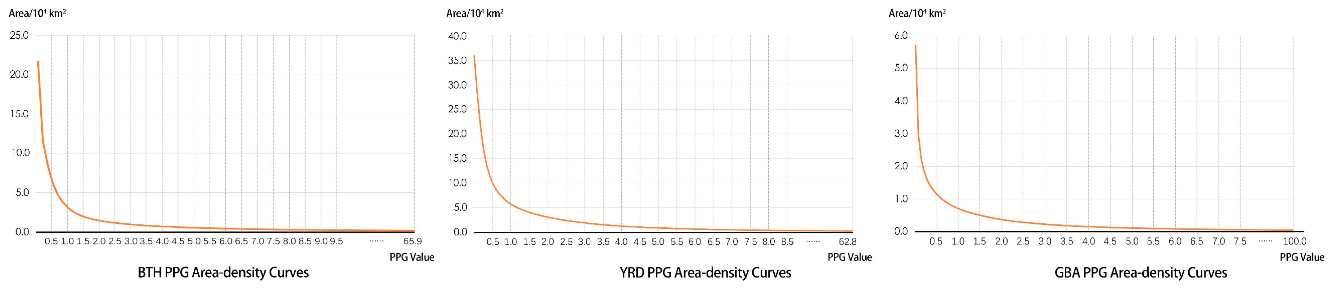
3.1.1. Boundary of Urban Clusters Identified by SEM

The population density, POI density, and GDP density change significantly near the boundaries of urban clusters. It is feasible and scientific to determine the threshold range of the urban agglomeration boundary by using its density change zone. Therefore, the study identifies the areas with high-density values of the three as urban clusters, where POI density recognition requires nuclear density analysis. It has been shown that smaller bandwidths can reflect local variation but may result in more false peaks. In comparison, larger bandwidths reflect overall variation but may miss or smooth out the spatial structure of urban cluster density [63]. After comparing the minimum outer rectangle method and the product of the square root method, the “Silverman rule of thumb” was taken to identify the kernel density bandwidth of POI data, which can effectively avoid spatial outliers [64]. Then, by combining the range and city level of each city cluster, the nuclear density analysis bandwidth interval of BTH, YRD, and GBA was determined; the results were 6.52 km, 8.46 km, and 8.81 km. The geometric margin method was used to categorize and display the generated POI kernel density maps via ArcGIS. The method allows the number of each category and the spacing between categories to be consistent. This is more balanced and eclectic than other methods; hence, the generated map has both the required information to be displayed and maintains a better visualization (Figure 3).

The area–density curves are drawn from the theoretical radius increment of the area enclosed by the $PPG$ index and its corresponding isoline within the study areas. As judged from the graph, when the $PPG$ index is 0.8, 1.4 and 1.1, respectively, the index contours of BTH, YRD, and GBA reach the critical point from dense to sparse (Figure 4). The three numbers are used as the initial urban dense area extraction threshold value. Considering that most urban clusters are developed and constructed areas, the independent patches over 1 km from the established areas are eliminated, and the neighboring independent patches greater than 5 km² are fused. The results show that the location of urban clusters is consistent with the core cities in each urban agglomeration (Figure 5). A continuous pattern has also been formed in the regions with complete urbanization. The urban cluster areas of BTH, YRD, and GBA are 22,629.00 km², 55,267.00 km², and 8995.00 km², respectively, accounting for 10.38%, 15.43%, and 16.01% of the administrative areas of the three regions, respectively.

3.1.2. Boundary of Urban Clusters Identified Using RSM

The spatial patterns of the four indexes are illustrated in Figure 6. In terms of denseness, all three areas show evident spatial divergence, and the high impervious surface distribution density values are concentrated in each urban cluster’s core cities. For example, BTH is bounded by the Taihang Mountains, and the results show a precipitous decline from east to west. The YRD shows a trend of decreasing from northeast to southwest. The GBA shows the decrease from the inside out with Nanhai, Baiyun, Huangpu, Panyu, and Shunde districts as the center. When it comes to contiguity, the GBA has the highest degree of continuous development and the lowest landscape heterogeneity of its land cover. The BTH is fragmented by artificial and natural divisions, resulting in a fragmented distribution of villages, towns, arable land, water bodies, woodlands, and grasslands, which need to form better connectivity, and has a low contiguity index as a whole. The YRD has an overall contiguous distribution of established towns, a relatively homogeneous landscape pattern, and an apparent development trend of contiguity. As for the gradient results, the urban development pattern of the three areas is spatially distributed in a “strip-like” manner, with a general trend of decreasing from the core cities to the periphery, which is consistent with the urban development orientation within each urban agglomeration. The typical features of these areas are lower slopes, better topographic conditions, and higher land productivity. Among them, the area east of the Taihang Mountains in BTH has a high degree of human interference. A diversity of land cover is irregularly distributed, leading to a high-value agglomeration of urban development gradients. The suitable development zones within each area are mainly distributed around town centers and road networks, eventually forming a pattern of several core development clusters radiating outward. Among them, Beijing–Tianjin–Rongfang in BTH, the Suzhou–Shanghai–Hangzhou corridor in the YRD, and the Pearl River coastline and its hinterland in GBA have more significant potential for contiguous development.

The denseness, contiguity, gradient, and development layers were weighted and superimposed to obtain the combined results. The natural breakpoint method was used to classify each into seven classes, and the high value areas (the two highest classes) were extracted accordingly. The fine patches smaller than 1 km² were removed to identify the extent of the urban cluster in each urban agglomeration (Figure 7).

The results show that the urban clusters in BTH are mainly distributed in the central urban areas of Beijing, Tianjin, Shijiazhuang, Tangshan, and Xingtai. There are isolated dotted areas (small- and medium-sized cities) in the periphery, such as Fangshan district in Beijing, Jinghai district in Tianjin, and Zhengding county in Shijiazhuang. In YRD, the urban clusters are mainly centered in Shanghai and extend north and south. They include Suzhou, Wuxi, Changzhou, Nanjing, and Zhenjiang to the north; and Jiaxing, Hangzhou and Ningbo to the south. The urbanization of these regions is more mature, and the contiguity of urban land is higher. In GBA, the urban clusters are concentrated in the U-shaped area around the mouth of the Pearl River, formed by Shenzhen, Dongguan, Guangzhou, Foshan, and Zhongshan.

3.1.3. Boundary of Urban Clusters Identified by TNM

As an effective metric to indicate inter-regional interactions, spatial accessibility is an expression that portrays how cities and regional systems perform agglomeration and diffusion functions. At the macro level, different urban isochronous zones based on accessibility representation can visualize the time range and convenience of enjoying central city services in different parts of the region. Each isochronous circle is composed of a combination of cities and their accessible hinterlands, forming a spatial association pattern between cities and hinterlands, cities and cities, and cities and regions within the urban cluster.

Comparing the urban isochrones with different time intervals, the isolines with a threshold of 20 min better reflect the geographic structure of urban functions in the metropolitan area of a single urban system. The isochronous circle with 20–40 min as the threshold better reflects the boundary, shape, and structure of the multi-city system at the regional scale. The 20 min isochronous circle is regarded as the primary reference basis in the study. The 30 min isochronous circle is used as a secondary reference variable to identify the spatial scope of urban agglomerations by examining the spatial association patterns of urban isochronous circles.

The findings reveal that the urban cluster exhibits a relatively continuous and compact spatial association pattern, a high degree of accessibility within the urban agglomerations, and an apparent spatial integration trend, thus realizing the spatial integration within the study areas (Figure 8). In terms of spatial distribution, these urban clusters are primarily located in plains and hilly areas, with a sound basis of natural environment and a relatively complete infrastructure network. They have different couplings with each urban agglomeration’s main economic and geographic spaces. The areas with good accessibility match the major urbanized areas, and some have formed large continuous urbanized geographical agglomerations. These areas generally have prime locations, improved infrastructure networks, higher density of population, and relatively active economic activities. On the edges of urban agglomerations such as Chengde City in BTH, Huangshan City, Fuyang City, and Huai’an City in YRD, several small-scale areas have high accessibility. However, these areas mostly show a scattered dotted distribution pattern, especially around the central city, forming a neighboring area with obvious distance decay. However, most of these areas show scattered dot-like distribution patterns, especially around the central cities forming adjacent areas with significant distance attenuation.

3.2. Comparison and Fusion of Identified Urban Clusters

The urban clusters depicted by the above three methods have the following characteristics: First, the spatial structures delineated by the three methods are similar. The area and scope of urban cluster boundaries extracted by the SEM and the RSM are similar and can be compared and verified. Second, in terms of the distribution of values, the three types of results show a general downward trend from urban centers to the edge of towns and finally to rural or ecological areas. In addition, the spatial distribution of high values obtained by the three methods is roughly the same, mainly centered on Beijing, Tianjin, Shijiazhuang, and Tangshan in BTH; Shanghai, Suzhou, Wuxi, Nanjing, Hangzhou, Jiaxing, and Ningbo in YRD; and the main urban areas in Shenzhen, Dongguan, Guangzhou, Zhongshan, and Foshan GBA. This indicates that all three methods can reflect the primary spatial structure of urban agglomerations and the coverage of urban clusters.

By comparison, it is found that the SEM better reflects the urban spatial function. However, its limitation is that some of the green areas and water bodies in its results are completely surrounded by patches of built-up areas. They need to be correctly extracted as built-up areas. In addition, the difference in the density of POI distribution produces some areas far from the core of urban agglomerations. This reflects that such data tend to ignore the interrelationship between cities when identifying the range of urban clusters. The RSM can give a more realistic and less detailed picture of the distribution of land cover. However, its harsh screening conditions cause its identified patches to be small in area and slightly fine-grained in morphology, with incomplete boundary contours and clearer jagged cross-sections; this makes it harder to produce a more accurate reference for delineating the boundaries. The method also tends to bring in redundant urban boundary lines, resulting in fragmented inner city spaces. The TNM strengthens the linkage between cities and regions and helps express town space development across administrative districts. Its drawback is that the results could be coarser, and numerous contiguous patches obscure the distribution of urban clusters. In addition, its shape is often radial along the road network, which is vulnerable to distortion in urban clusters’ shape.

The urban clusters obtained by each of the three methods were assigned a score of one (non-urban clusters were assigned a score of zero), and the results were superimposed with equal weights in ArcGIS. A hotspot analysis was performed on the total score (out of three). The standard deviation multiplier Z scores calculated for each sampling grid and their corresponding P values at 90%, 95%, and 99% confidence intervals were calculated analytically under the first-order Queen neighborhood space weights. Under the premise of passing the hypothesis test, if the Z score is positive, the sampling grid has a relatively high index of urban dense area characteristics when compared with the surrounding grid and will be identified as a hot spot (Figure 9). A higher Z-score indicates a higher degree of clustering, while the opposite indicates a cold spot area. A failure of the hypothesis test means that the clustering of values is not significant.

The results of the data fusion method (Figure 10) show that the area of the identified urban compact area is 11,992.00 km², 29,832.00 km², and 5720.00 km², accounting for 5.50%, 8.33%, and 10.23% of the area of the three urban agglomerations. The new boundary is effectively corrected compared to the three methods mentioned above. On the one hand, the urban cluster boundaries delineated by the SEM and RSM have many overlapping parts in space. These areas are strengthened in the results after the data fusion, which enriches the internal spatial details of the urban cluster, especially in the central urban areas of Beijing, Tianjin, Shijiazhuang, Shanghai, Suzhou, Hangzhou, Shenzhen, Guangzhou, and Dongguan. On the other hand, the results obtained from the TNM contribute to smoothing the spatial fragmentation of urban areas and complementing the spatial linkage structure between cities, such as the Xiong’an New Zone between Beijing and Tianjin, the Jiaxing zone between Shanghai and Hangzhou, and the Dongguan zone between Guangzhou and Shenzhen, which are enhanced in the integrated identification.

3.3. Verification of Urban Cluster Identifications

Determining the accuracy of urban cluster identification is relatively difficult. The built-up areas of Chinese cities in 2020 (http://www.resdc.cn/Datalist1.aspx?FieldTyepID=1,3, accessed on 23 January 2023) was transformed into point elements in GIS. The nuclear density analysis was performed to characterize the density distribution of urban land and used to conduct a consistency test with urban clusters. The dataset was developed using the United Nations built-up area standards and produced with high-precision data sources and high-precision data products to meet the current requirements of urban sustainability research. A total of 6000 random points (each urban agglomeration contains 1000 test points and 1000 validation points) are randomly sampled within the three urban agglomerations to validate the urban cluster area identified by different methods. The judgments are supplemented with a visual interpretation based on a Google Earth high-resolution image to obtain the reference attributes of the validation points to ensure the accuracy of the attribute acquisition. The confusion matrix is shown in

Table 3. Confusion matrix.

	Case	BTH		YRD		GBA
Methods		OA	Kappa Efficient	OA	Kappa Efficient	OA	Kappa Efficient
SEM		55.97%	0.4435	52.91%	0.4203	63.58%	0.5748
RSM		44.45%	0.3524	20.34%	0.1830	27.84%	0.2473
TNM		33.72%	0.3141	28.35%	0.2212	31.17%	0.2958
Data fusion		90.11%	0.8115	81.40%	0.6807	84.52%	0.7260

based on the verification results. Overall accuracy (OA) is the percentage of the number of all random points successfully validated. The Kappa coefficient for consistency testing can be used to measure classification accuracy. This means that the higher the overall accuracy and Kappa coefficient, the better the classification results conform to the physical truth, indicating higher recognition accuracy.

Differences exist in the accuracy of urban cluster area identification for different methods. The average value of the OA of the urban cluster boundaries delineated by the SEM, RSM, and TNM were all between 20.34% and 63.58%. Among them, the identification accuracy of the SEM was relatively high, which was especially clear in the GBA. In terms of the accuracy effect, the maximum improvement of the delineated boundaries of the three urban clusters after data fusion are 56.39%, 61.06%, and 56.58%. The Kappa coefficients of the first three methods are between 0.1830 and 0.5748, with the GBA showing the highest Kappa coefficient overall. The Kappa coefficients after data fusion improved to 0.8115 (BTH), 0.6807 (YRD), and 0.7260 (GBA). With respect to Kappa coefficient enhancement, the fusion of the three data types can more accurately demarcate the boundaries of urban cluster areas. The data fusion method combines the advantages of various types of data and methods to promote the reflection of the structural integrity within urban agglomeration. This can strengthen and polarize the location of the core urban area so that the identified spatial area is more in line with the development status and better reflects the urban clusters’ more detailed neighborhoods, making the delineated boundary complete and accurate. A local Google satellite map comparison is performed for some locations with doubtful validation (Figure 11). These areas are primarily urban–rural fringe and metropolitan fringe areas. The overlapping of artificial and natural landscapes makes them the “leading edge” of urban expansion, as well as the “pioneer area” of rural urbanization. The intersection of the two different nature patches generates dynamic marginal land types, which can easily cause identification errors.

4. Discussion

4.1. Method Comparison

The urban cluster areas of China’s three major urban agglomerations were identified using different methods, including SEM, RSM, and TNM. Following an analysis of the strengths and weaknesses of each data type and method, the GIS platform was utilized for data fusion and hotspot analysis in order to re-detect town-dense areas. Comparative validation was also conducted to further confirm the accuracy of the data fusion method, which was found to be higher than that of the aforementioned methods and more effective in identifying urban clusters. These findings are in line with those of other researchers. Zhou et al. used POI data and night light images to extract the actual boundaries of the three major urban agglomerations in China. The detected areas accounted for 20.92–25.42% of the total area of each urban agglomeration [51]. On this basis, Xiong et al. combined Tencent migration data, extracted the spatial structure of the Greater Bay Area poly center, and compared it with overall planning to achieve a Kappa of 0.8871 [2]. The identification of the urban clusters in the study shows that their area accounts for 5.50–10.23% of the three major urban agglomerations; their OA and Kappa reached 90.11% and 0.8115. Compared to previous research, the scope of the urban clusters identified has been refined with a greater emphasis on the actual developmental status of cities rather than solely considering the physical boundaries of urban agglomerations. In terms of accuracy, the results are comparable to those of identifying the multicenter structure of urban agglomerations and offer a more comprehensive reflection of the spatial distribution of regional centers and their hinterlands [39,51]. This is attributed to the multi-dimensional characteristic mapping of social and economic factors, urban land use, and communication connections. In terms of data fusion, previous studies [2,39] have employed wavelet transforms for pixel-level image fusion, which can preserve essential information from multiple original images. In comparison, “hotspot analysis” is a more convenient and efficient method that achieves a comprehensive examination of nearby environmental features, better satisfying the connotation requirements of densely populated urban areas. The multi-source fusion of data plays a crucial role in the rapid delineation of urban cluster boundaries. The resulting physical boundaries are more distinct and well-defined as compared to those obtained in previous studies. Moreover, this approach can be extended to identify urban clusters in other highly urbanized regions. The difference in data sources and processing methods is the primary reason for the improved accuracy. Among these methods, SEM is commonly used for the identification and evaluation of traditional polycentric spatial structures, but it has a high degree of subjectivity. Furthermore, the point-like area on the periphery of the high-value area is spatially fragmented from the central area of the urban agglomeration. The proposed method highlights the intrinsic functional development and land use distribution of urban agglomerations by integrating the advantages of transportation accessibility in expressing inter-town connections. This method provides a more accurate range of urban clusters and avoids subjectivity and uncertainty in the identification process. Additionally, the built-up areas of BTH, YRD, and GBA in 2022 are 6980.06 km², 15,744.86 km², and 4310.41 km², respectively. The area identified after data fusion is larger than the original data. Therefore, the spatial area of urban clusters obtained by data fusion is more aligned with the “spatial radiation range of urban agglomeration”. Overall, in this study, three types of spatial data are fused to enable the rapid identification and extraction of actual boundaries for urban clusters within each region based on a unified standard. The resulting boundary profile is more specific and clearer than previous studies, providing a novel method and perspective for regional spatial research. Additionally, through case studies on China’s three major urban agglomerations, the proposed method system is demonstrated to be applicable in different regions, which underscores its significant value. It facilitates understanding of the differences between the actual development status of urban agglomerations and spatial planning, making a practical contribution to formulating regional spatial development policies.

4.2. Limitations and Potential Solutions

The proposed methods are not dependent on administrative divisions. In the absence of standardized results for comparison, the intercomparison of the results can also demonstrate the validity to some extent. However, there are three related limitations that need to be addressed in further studies. First, there is a close connection between towns in urban clusters and a strong interaction between urban and rural areas. This effect is reflected not only in the economy, land use, and transportation but also in many aspects of history, society, and culture. However, this close relationship has not yet been fully realized. Moreover, GDP, population density, night lights, and other factors vary considerably between cities, which may lead to a higher index of characteristics in rural areas around some metropolitan regions than in the built-up areas of less developed cities [29]. Thus, it is necessary to further verify whether the proposed method applies to urban agglomerations with different development levels. Second, with the development of urban commuting, the organizational structure and operation of socio-economic activities have changed profoundly, and the spatiotemporal relationships tend to be redefined. The analysis of commuting data relies on the choice of origin and destination locations and the selected transportation means, which introduces higher uncertainty. Furthermore, traffic “flows” are challenging to characterize directly due to the complex drivers of urban linkages [65]. Therefore, the highlight of future research breakthroughs is the objective measurement of human exchange links between cities. The use of mobile phone signaling data to measure intercity commuting and enhance the characteristic expression of the supply–demand relationship between transportation accessibility and functionality connections is suggested. Third, the SEM uses the index value corresponding to the sudden increase in the area of urban clusters as the segmentation threshold. Such an extraction model is more suitable for monocentric urban areas. However, its applicability to polycentric urban areas is doubtful since the results are likely to be larger than the actual urban clusters [66]. Faced with the trend of spatial networking, the definition of future urban clusters should be based on a comprehensive and integrated approach. It is feasible to combine the generation of iso-lines for urban cluster attributes with the localized contour tree method to identify the multiple centers and hierarchical structure of urban clusters. Furthermore, integrated simulations that combine the advantages of social, economic, and natural indicators and gravitational models should be enhanced. Additionally, there is a need to improve the accuracy and timeliness of data collection. For instance, unmanned aerial vehicles (UAVs) are effective tools for measuring urban surface construction. They can play a practical role in the fine-grained monitoring of urban clusters through multi-angle observation, high dynamic range imaging technology, and more advanced sensors and analysis methods [67].

4.3. How Urban Clusters Contribute

In the context of setting regional development goals and assessing actual development levels, the definition of the spatial scope of urban clusters has a considerable impact on evaluating the development status and level of any given region. The assessment of high-level and high-quality development of urban clusters, based on actual growth boundaries, serves as the initial point for initiating spatial planning. Accordingly, this enables the determination of an appropriate spatial scope for urban clusters, evaluation of basic conditions, and measurement of resource and environmental sustainability. Furthermore, the overall layout of the population and urbanization, urban–rural coordination, the industrial division of labor, infrastructure construction, and ecological environmental protection can be taken into consideration as well.

5. Conclusions and Prospects

Determining the developmental boundaries of core urban agglomeration areas is crucial for optimizing resource allocation and promoting integration processes. In this study, the urban clusters of three major urban agglomerations were identified using the SEM, RSM, TNM, and data fusion methods. The conclusions drawn from different identification methods can provide valuable insights. Using a comprehensive comparative analysis of various data partitioning methods for the delineation of urban agglomeration boundaries, the SEM method was found to have an OA of 57.49% and a Kappa coefficient of 0.4795, while the RSM method had an OA of 30.88% and a Kappa coefficient of 0.2609. The TNM method demonstrated an OA of 31.08% and a Kappa coefficient of 0.2770. Finally, the data fusion method yielded an OA of 85.34% and a Kappa coefficient of 0.7394. These results suggest that the data fusion method is particularly effective in capturing the unique characteristics of each data source, thus improving the accuracy of urban cluster boundary delineation. Furthermore, this method is especially useful in determining the actual area of urban agglomerations that are actively utilized, having significant implications for practical urban planning and management practices.

First, the SEM reflects the strength of human socio-economic activities and expresses the actual level of production and living. The POI data can serve as an effective tool for reflecting the economic agglomeration and diffusion characteristics, as it highlights the radiation effect of core cities in urban clusters. Moreover, its use enables the extraction and identification of boundaries at a large scale with high accuracy, while keeping costs low. In comparison, the proposed method identifies the range and shape of dense urban areas closest to the results obtained by the data fusion method. The RSM can accurately extract and identify the boundaries of urban clusters, while effectively characterizing urban pattern, scale, land use, and spatial functions by integrating both natural and artificial elements at a broad scale. This can guide the intensive development of urban spaces. However, due to its multidimensional and stringent filtering criteria, RSM often neglects semi-urbanized spaces, leading to more detailed but finer-grained identification results. The TNM, on the other hand, can better capture the more influential neighborhoods of urban agglomerations and the connecting axes between cities. The method can effectively demonstrate the urban hierarchical system planned for each urban cluster. Identifying rudimentary branch axes can further aid in observing potential expansion directions of dense urban areas and exploring opportunities for developing small towns in urban proximities. However, the results are relatively coarse, and the linear connection zones between towns are likely to contain areas where towns are less intensively built up. The boundaries of urban clusters identified by the three methods are all much smaller than the administrative area of urban agglomerations. Their areas range from 0.88% to 21.73% of the planned areas of each urban agglomeration.

Hotspot analysis is applied to the fusion results, enhancing the identification of high and low clustering cases of eigenvalues in the local area. This method is based on the second law of geography, which compensates for the subjective influence of traditional methods that require artificial thresholds and avoids the interference of the incompleteness of element capture on the identification results. The area of the identified urban clusters’ boundary is similar to that obtained by the above three methods, allowing for comparison and verification. Furthermore, the urban clusters extracted by the data fusion method are smaller in size and have a more concentrated and continuous pattern, with a good representation of the overall contour and internal details of the urban clusters. In contrast, the urban clusters identified by other methods tend to be either too fine-grained or too broad in scope. A comparison with actual surface conditions observed via Google satellite imagery demonstrates the need for further visual optimization to enhance identification accuracy for urban clusters, even after the integration of various datasets. Visual optimization should address two aspects, namely identifying and correcting misclassified objects in the verification samples and addressing objects with inconsistent classification results in their surroundings.

Finally, in terms of accuracy, the SEM has the highest OA for identifying urban clusters in BTH (55.97%), YRD (52.91%), and GBA (63.58%), with kappa coefficients ranging from 0.4435 to 0.5748. The TNM has a relatively high accuracy in identifying urban clusters in BTH (33.72%). The RSM has the lowest average OA with 30.88% and an average Kappa coefficient of 0.2609. Following data fusion, the average overall accuracy (OA) of urban clusters was calculated to be 85.34%, with the average Kappa coefficient increasing to 0.7394. These findings suggest that the fused method is more effective and objective. To enhance the persuasiveness of the results and verify the study’s correctness, the results were compared with those of previous studies on the identification of urban dense area boundaries. The comparison further confirmed the correctness of this study and increased the persuasiveness of the boundary identification.

The identification method for urban clusters based on data fusion breaks the constraint of using administrative districts as research units and instead discriminates all urban units as a whole, providing an objective reflection of the scope of dense urban areas and avoiding the blind expansion of urban agglomeration boundaries without considering reality. This method can be extended to other spatial structures of towns in different stages of growth, concretizing the heterogeneity of inter-city relations. As an integrated entity, urban clusters often undergo indiscriminate expansion of urban land use, which occurs alongside the rapid development of core cities. Therefore, precise and rational control over boundary growth is conducive to promoting the free flow of factors and optimizing spatial structures, ultimately improving the efficiency of urban cluster management and acting as a reference for macro-planning and local governance. The aforementioned issues are manifested through restrictions on urban sprawl and the optimization of utilization efficiency for existing urban land, with a focus on defining the development scope of construction land to prevent inefficient and indiscriminate expansion. Additionally, preserving ecological and agricultural land is critical to achieve rational allocation of human activities, land use, and scenic quality. Given that urban land expansion is a dynamic process with significant variations across different stages, regular and dynamic delineation and adjustment of urban development boundaries is necessary. Furthermore, exploring the economic, social, policy, and environmental mechanisms and evolution prediction of this dynamic system is warranted.

References

1. Li, L.; Ma, S.; Zheng, Y.; Xiao, X. Integrated Regional Development: Comparison of Urban Agglomeration Policies in China. Land Use Policy 2022, 114, 105939. [Google Scholar] [CrossRef]
2. He, X.; Cao, Y.; Zhou, C. Evaluation of Polycentric Spatial Structure in the Urban Agglomeration of the Pearl River Delta (Prd) Based on Multi-Source Big Data Fusion. Remote Sens. 2021, 13, 3639. [Google Scholar] [CrossRef]
3. Veneri, P. City Size Distribution across the OECD: Does the Definition of Cities Matter? Comput. Environ. Urban Syst. 2016, 59, 86–94. [Google Scholar] [CrossRef]
4. Yu, Q.; Li, M.; Li, Q.; Wang, Y.; Chen, W. Economic Agglomeration and Emissions Reduction: Does High Agglomeration in China’s Urban Clusters Lead to Higher Carbon Intensity? Urban Clim. 2022, 43, 101174. [Google Scholar] [CrossRef]
5. Ascher, C.S.; Geddes, P.; The Outlook Tower Association, E. Cities in Evolution. Land Econ. 1951, 27, 83. [Google Scholar] [CrossRef]
6. Gottmann, J. The Evolution of the Concept of Territory. Soc. Sci. Inf. 1975, 14, 29–47. [Google Scholar] [CrossRef]
7. Thacher, P.S. Ecumenopolis, The Inevitable City of the Future, by C. A. Doxiadis & J. G. Papaioannou. Athens Center of Ekistics, 24 Stratiotikou Syndesmou Street, Athens 136, Greece: Xxviii + 469 Pp., 153 Figs Incl. Numerous Maps, 23.5 × 15.6 × 2.5 Cm, Thick Paper Cove. Environ. Conserv. 1975, 2, 315–317. [Google Scholar] [CrossRef]
8. Gottmann, J. Megalopolis or the Urbanization of the Northeastern Seaboard. Econ. Geogr. 1957, 33, 189. [Google Scholar] [CrossRef]
9. Denis, P.-Y. Hall, Peter (1984) The World Cities. London, Weidenfeld and Nicolson, Third Edition, 276 P. Cah. Geogr. Que. 2012, 29, 441. [Google Scholar] [CrossRef]
10. Friedmann, J.; Miller, J. THE URBAN FIELD. J. Am. Plan. Assoc. 1965, 31, 312–320. [Google Scholar] [CrossRef]
11. O’Neill, P. Global City-Regions: Trends, Theory, Policy. Area 2003, 35, 326–327. [Google Scholar] [CrossRef]
12. Fang, C. The Basic Law of the Formation and Expansion in Urban Agglomerations. J. Geogr. Sci. 2019, 29, 1699–1712. [Google Scholar] [CrossRef]
13. Lv, Q.; Dou, Y.; Niu, X.; Xu, J.; Xu, J.; Xia, F. Urban Land Use and Land Cover Classification Using Remotely Sensed Sar Data through Deep Belief Networks. J. Sens. 2015, 2015, 538063. [Google Scholar] [CrossRef]
14. Fragkias, M.; Seto, K.C. Evolving Rank-Size Distributions of Intra-Metropolitan Urban Clusters in South China. Comput. Environ. Urban Syst. 2009, 33, 189–199. [Google Scholar] [CrossRef]
15. Wheeler, J.O.; Mitchelson, R.L. Information Flows among Major Metropolitan Areas in the United States. Ann. Assoc. Am. Geogr. 1989, 79, 523–543. [Google Scholar] [CrossRef]
16. Wang, H.; Deng, Y.; Tian, E.; Wang, K. A Comparative Study of Methods for Delineating Sphere of Urban Influence: A Case Study on Central China. Chin. Geogr. Sci. 2014, 24, 751–762. [Google Scholar] [CrossRef]
17. Huff, D.L.; Lutz, J.M. Ireland’s Urban System. Econ. Geogr. 1979, 55, 196. [Google Scholar] [CrossRef]
18. Van Arjen Klink, H.; Van Den Berg, G.C. Gateways and Intermodalism. J. Transp. Geogr. 1998, 6, 1–9. [Google Scholar] [CrossRef]
19. Wang, T.; Zhang, G.; Li, P.; Li, F.; Guo, X. Analysis on the Driving Factors of Urban Expansion Policy Based on DMSP/OLS Remote Sensing Image. Cehui Xuebao/Acta Geod. Cartogr. Sin. 2018, 47, 1466. [Google Scholar] [CrossRef]
20. Tannier, C.; Thomas, I. Defining and Characterizing Urban Boundaries: A Fractal Analysis of Theoretical Cities and Belgian Cities. Comput. Environ. Urban Syst. 2013, 41, 234–248. [Google Scholar] [CrossRef]
21. Liu, X.; Derudder, B.; Wang, M. Polycentric Urban Development in China: A Multi-Scale Analysis. Environ. Plan. B Urban Anal. City Sci. 2018, 45, 953–972. [Google Scholar] [CrossRef]
22. Li, F.; Yan, Q.; Bian, Z.; Liu, B.; Wu, Z. A Poi and Lst Adjusted Ntl Urban Index for Urban Built-up Area Extraction. Sensors 2020, 20, 2918. [Google Scholar] [CrossRef]
23. Adolphson, M. Estimating a Polycentric Urban Structure. Case Study: Urban Changes in the Stockholm Region 1991–2004. J. Urban Plan. Dev. 2009, 135, 19–30. [Google Scholar] [CrossRef]
24. Cao, W.; Dong, L.; Cheng, Y.; Wu, L.; Guo, Q.; Liu, Y. Constructing Multi-Level Urban Clusters Based on Population Distributions and Interactions. Comput. Environ. Urban Syst. 2023, 99, 101897. [Google Scholar] [CrossRef]
25. Georg, I.; Blaschke, T.; Taubenböck, H. Spatial Delineation of Urban Corridors in North America: An Approach Incorporating Fuzziness Based on Multi-Source Geospatial Data. Cities 2023, 133, 104129. [Google Scholar] [CrossRef]
26. Elvidge, C.D.; Baugh, K.E.; Dietz, J.B.; Bland, T.; Sutton, P.C.; Kroehl, H.W. Radiance Calibration of DMSP-OLS Low-Light Imaging Data of Human Settlements. Remote Sens. Environ. 1999, 68, 77–88. [Google Scholar] [CrossRef]
27. Dai, X.; Jin, J.; Chen, Q.; Fang, X. On Physical Urban Boundaries, Urban Sprawl, and Compactness Measurement: A Case Study of the Wen-Tai Region, China. Land 2022, 11, 1637. [Google Scholar] [CrossRef]
28. Hu, S.; Tong, L.; Frazier, A.E.; Liu, Y. Urban Boundary Extraction and Sprawl Analysis Using Landsat Images: A Case Study in Wuhan, China. Habitat Int. 2015, 47, 183–195. [Google Scholar] [CrossRef]
29. Zhang, X.; Du, S.; Zhou, Y.; Xu, Y. Extracting Physical Urban Areas of 81 Major Chinese Cities from High-Resolution Land Uses. Cities 2022, 131, 104061. [Google Scholar] [CrossRef]
30. Van de Voorde, T.; Jacquet, W.; Canters, F. Mapping Form and Function in Urban Areas: An Approach Based on Urban Metrics and Continuous Impervious Surface Data. Landsc. Urban Plan. 2011, 102, 143–155. [Google Scholar] [CrossRef]
31. Li, X.; Zhou, Y.; Zhu, Z.; Liang, L.; Yu, B.; Cao, W. Mapping Annual Urban Dynamics (1985–2015) Using Time Series of Landsat Data. Remote Sens. Environ. 2018, 216, 674–683. [Google Scholar] [CrossRef]
32. Luqman, M.; Rayner, P.J.; Gurney, K.R. Combining Measurements of Built-up Area, Nighttime Light, and Travel Time Distance for Detecting Changes in Urban Boundaries: Introducing the BUNTUS Algorithm. Remote Sens. 2019, 11, 2969. [Google Scholar] [CrossRef]
33. Lou, G.; Chen, Q.; He, K.; Zhou, Y.; Shi, Z. Using Nighttime Light Data and POI Big Data to Detect the Urban Centers of Hangzhou. Remote Sens. 2019, 11, 1821. [Google Scholar] [CrossRef]
34. He, X.; Zhu, Y.; Chang, P.; Zhou, C. Using Tencent User Location Data to Modify Night-Time Light Data for Delineating Urban Agglomeration Boundaries. Front. Environ. Sci. 2022, 10, 860365. [Google Scholar] [CrossRef]
35. Zhang, X.; Wang, H.; Ning, X.; Zhang, X.; Liu, R.; Wang, H. Identification of Metropolitan Area Boundaries Based on Comprehensive Spatial Linkages of Cities: A Case Study of the Beijing–Tianjin–Hebei Region. ISPRS Int. J. Geo-Inf. 2022, 11, 396. [Google Scholar] [CrossRef]
36. Fang, C.; Yu, D. Urban Agglomeration: An Evolving Concept of an Emerging Phenomenon. Landsc. Urban Plan. 2017, 162, 126–136. [Google Scholar] [CrossRef]
37. Takahashi, K.I.; Terakado, R.; Nakamura, J.; Adachi, Y.; Elvidge, C.D.; Matsuno, Y. In-Use Stock Analysis Using Satellite Nighttime Light Observation Data. Resour. Conserv. Recycl. 2010, 55, 196–200. [Google Scholar] [CrossRef]
38. Stokes, E.C.; Seto, K.C. Characterizing Urban Infrastructural Transitions for the Sustainable Development Goals Using Multi-Temporal Land, Population, and Nighttime Light Data. Remote Sens. Environ. 2019, 234, 111430. [Google Scholar] [CrossRef]
39. Zhang, S.; Wei, H. Identification of Urban Agglomeration Spatial Range Based on Social and Remote-Sensing Data—For Evaluating Development Level of Urban Agglomeration. ISPRS Int. J. Geo-Inf. 2022, 11, 456. [Google Scholar] [CrossRef]
40. Fang, C. New Structure and New Trend of Formation and Development. Sci. Geogr. Sin. 2019, 31, 1025–1034. [Google Scholar] [CrossRef]
41. Zhang, Y.; Mao, W.; Zhang, B. Distortion of Government Behaviour under Target Constraints: Economic Growth Target and Urban Sprawl in China. Cities 2022, 131, 104009. [Google Scholar] [CrossRef]
42. Hosseinpour, H.; Samadzadegan, F.; Javan, F.D. CMGFNet: A Deep Cross-Modal Gated Fusion Network for Building Extraction from Very High-Resolution Remote Sensing Images. ISPRS J. Photogramm. Remote Sens. 2022, 184, 96–115. [Google Scholar] [CrossRef]
43. Wang, M.; Song, Y.; Wang, F.; Meng, Z. Boundary Extraction of Urban Built-Up Area Based on Luminance Value Correction of NTL Image. IEEE J. Sel. Top. Appl. Earth Obs. Remote Sens. 2021, 14, 7466–7477. [Google Scholar] [CrossRef]
44. Wang, S.; Huang, L.; Xu, X.; Li, J. Spatio-Temporal Variation Characteristics of Ecological Space and Its Ecological Carrying Status in Mega-Urban Agglomerations. Dili Xuebao/Acta Geogr. Sin. 2022, 77, 164–181. [Google Scholar] [CrossRef]
45. Yang, J.; Huang, X. The 30m Annual Land Cover Dataset and Its Dynamics in China from 1990 to 2019. Earth Syst. Sci. Data 2021, 13, 3907–3925. [Google Scholar] [CrossRef]
46. Yu, M.; Guo, S.; Guan, Y.; Cai, D.; Zhang, C.; Fraedrich, K.; Liao, Z.; Zhang, X.; Tian, Z. Spatiotemporal Heterogeneity Analysis of Yangtze River Delta Urban Agglomeration: Evidence from Nighttime Light Data (2001–2019). Remote Sens. 2021, 13, 1235. [Google Scholar] [CrossRef]
47. Zheng, Y.; He, Y.; Zhou, Q.; Wang, H. Quantitative Evaluation of Urban Expansion Using NPP-VIIRS Nighttime Light and Landsat Spectral Data. Sustain. Cities Soc. 2022, 76, 103338. [Google Scholar] [CrossRef]
48. Zhou, Y.; Li, C.; Zheng, W.; Rong, Y.; Liu, W. Identification of Urban Shrinkage Using NPP-VIIRS Nighttime Light Data at the County Level in China. Cities 2021, 118, 103373. [Google Scholar] [CrossRef]
49. Zhao, P.; Jia, T.; Qin, K.; Shan, J.; Jiao, C. Statistical Analysis on the Evolution of OpenStreetMap Road Networks in Beijing. Phys. A Stat. Mech. Its Appl. 2015, 420, 59–72. [Google Scholar] [CrossRef]
50. Huang, W.; Zhang, D.; Mai, G.; Guo, X.; Cui, L. ISPRS Journal of Photogrammetry and Remote Sensing Learning Urban Region Representations with POIs and Hierarchical Graph Infomax. ISPRS J. Photogramm. Remote Sens. 2023, 196, 134–145. [Google Scholar] [CrossRef]
51. Zhou, L.; Zhou, Q.; Yang, F. Identification of Urban Agglomeration Boundary Based on POI and NPP/VIIRS Night Light Data. Prog. Geogr. 2019, 38, 840–850. [Google Scholar] [CrossRef]
52. Peng, J.; Hu, Y.; Liu, Y.; Ma, J.; Zhao, S. A New Approach for Urban-Rural Fringe Identification: Integrating Impervious Surface Area and Spatial Continuous Wavelet Transform. Landsc. Urban Plan. 2018, 175, 72–79. [Google Scholar] [CrossRef]
53. Shahtahmassebi, A.R.; Song, J.; Zheng, Q.; Blackburn, G.A.; Wang, K.; Huang, L.Y.; Pan, Y.; Moore, N.; Shahtahmassebi, G.; Sadrabadi Haghighi, R.; et al. Remote Sensing of Impervious Surface Growth: A Framework for Quantifying Urban Expansion and Re-Densification Mechanisms. Int. J. Appl. Earth Obs. Geoinf. 2016, 46, 94–112. [Google Scholar] [CrossRef]
54. Li, G.; CAO, Y.; He, Z.; He, J.; Cao, Y.; Wang, J.; Fang, X. Understanding the Diversity of Urban–Rural Fringe Development in a Fast Urbanizing Region of China. Remote Sens. 2021, 13, 2373. [Google Scholar] [CrossRef]
55. Clark, C. Urban Population Pensities. J. R. Stat. Soc. Ser. A (Gen.) 1898, 114, 490–496. [Google Scholar] [CrossRef]
56. Zhang, D.; Liu, J. Study on the Model of Regional Differentiation of Land Use Degree in China. J. Nat. Resour. 1997, 12, 105–111. [Google Scholar]
57. Qin, H.; Zhang, F.; Du, Z.; Renyi, L. The Evaluate of Urban Development in Zhejiang Province Based on DMSP/OLS Nighttime Light Data. J. Zhejiang Univ. Ed. 2017, 44, 640–648. [Google Scholar] [CrossRef]
58. Weiss, D.J.; Nelson, A.; Gibson, H.S.; Temperley, W.; Peedell, S.; Lieber, A.; Hancher, M.; Poyart, E.; Belchior, S.; Fullman, N.; et al. A Global Map of Travel Time to Cities to Assess Inequalities in Accessibility in 2015. Nat. Publ. Gr. 2018, 553, 333–336. [Google Scholar] [CrossRef]
59. Chen, W. Identifying the Spatial Scope of Megaregions in China from the Perspective of Accessibility. Geogr. Res. 2020, 39, 2808–2820. [Google Scholar] [CrossRef]
60. Getis, A.; Ord, J.K. The Analysis of Spatial Association by Use of Distance Statistics. Perspect. Spat. Data Anal. 1992, 24, 127–145. [Google Scholar] [CrossRef]
61. Yang, Y.; Xiao, P.; Feng, X.; Li, H. ISPRS Journal of Photogrammetry and Remote Sensing Accuracy Assessment of Seven Global Land Cover Datasets over China. ISPRS J. Photogramm. Remote Sens. 2017, 125, 156–173. [Google Scholar] [CrossRef]
62. Stehman, S.V. Selecting and Interpreting Measures of Thematic Classification Accuracy. Remote Sens. Environ. 1997, 62, 77–89. [Google Scholar] [CrossRef]
63. Schindler, N.H.A. Bandwidth Selection for Kernel Density Estimation: A Review of Fully Automatic Selectors. AStA Adv. Stat. Anal. 2013, 97, 403–433. [Google Scholar] [CrossRef]
64. Schucany, W.R. Locally Optimal Window Widths for Kernel Density Estimation with Large Samples. Stat. Probab. Lett. 1989, 7, 401–405. [Google Scholar] [CrossRef]
65. Yao, Z.; Ye, K.; Xiao, L.; Wang, X. Radiation Effect of Urban Agglomeration’s Transportation Network: Evidence from Chengdu–Chongqing Urban Agglomeration, China. Land 2021, 10, 520. [Google Scholar] [CrossRef]
66. Liu, X.; Ning, X.; Wang, H.; Wang, C.; Zhang, H.; Meng, J. A Rapid and Automated Urban Boundary Extraction Method Based on Nighttime Light Data in China. Remote Sens. 2019, 11, 1126. [Google Scholar] [CrossRef]
67. Li, X.; Levin, N.; Xie, J.; Li, D. Monitoring Hourly Night-Time Light by an Unmanned Aerial Vehicle and Its Implications to Satellite Remote Sensing. Remote Sens. Environ. 2020, 247, 111942. [Google Scholar] [CrossRef]
Figure 1. Beijing–Tianjin–Hebei (BTH) Urban Agglomeration, Yangtze River Delta (YRD) Urban Agglomeration, Guangdong–Hong Kong–Macao Greater Bay Area (GBA), China.
Land 12 01058 g001
Figure 2. Technical route of the study.
Land 12 01058 g002
Figure 3. The Spatial pattern of population density, POI kernel density, and GDP intensity.
Land 12 01058 g003
Figure 4. PPG area–density curves.
Land 12 01058 g004
Figure 5. Spatial area of urban clusters identified using SEM.
Land 12 01058 g005
Figure 6. The spatial pattern of denseness, continuity, gradient, and development indexes.
Land 12 01058 g006
Figure 7. Spatial area of urban clusters identified by RSM.
Land 12 01058 g007
Figure 8. Spatial area of urban clusters identified by TNM.
Land 12 01058 g008
Figure 9. Hot spot analysis of data fusion results.
Land 12 01058 g009
Figure 10. Comparison of results of urban clusters identified by different methods.
Land 12 01058 g010
Figure 11. Identification results of data fusion compared with Google images.
Land 12 01058 g011