Article

Land Subsidence Susceptibility Mapping Using Interferometric Synthetic Aperture Radar (InSAR) and Machine Learning Models in a Semiarid Region of Iran

by
Hamidreza Gharechaee
1,
Aliakbar Nazari Samani
1,*,
Shahram Khalighi Sigaroodi
1,
Abolfazl Baloochiyan
2,
Maryam Sadat Moosavi
3,
Jason A. Hubbart
4 and
Seyed Mohammad Moein Sadeghi
5,*
1
Reclamation of Arid and Mountainous Regions Department, Faculty of Natural Resources, University of Tehran, Karaj 3158577871, Iran
2
Faculty of Mechanical Engineering, Ozyegin University, Istanbul 34794, Turkey
3
Department of Arid and Desert Regions Management, School of Natural Resources & Desert Studies, Yazd University, Yazd 8915818411, Iran
4
Division of Forestry and Natural Resources, Davis College of Agriculture, Natural Resources and Design, West Virginia University, Percival Hall, Morgantown, WV 26506, USA
5
School of Forest, Fisheries and Geomatics Sciences, University of Florida, Gainesville, FL 32611, USA
*
Authors to whom correspondence should be addressed.
Land 2023, 12(4), 843; https://doi.org/10.3390/land12040843
Submission received: 15 February 2023 / Revised: 25 March 2023 / Accepted: 4 April 2023 / Published: 7 April 2023

Abstract

:
Most published studies identify groundwater extraction as the leading cause of land subsidence (LS). However, the causes of LS are not only attributable to groundwater extraction. Other land-use practices can also affect the occurrence of LS. In this study, radar interferometric techniques and machine learning (ML) models were used for the prediction, susceptibility zoning, and prioritization of influential variables in the occurrence of LS in the Bakhtegan basin. The LS rate was characterized by applying an interferometric synthetic aperture radar (InSAR). The recursive feature elimination (RFE) method was used to detect and select the dominant combination of indicators to prepare an LS susceptibility map. Three ML models, including random forest (RF), k-nearest neighbors (KNN), and classification and regression trees (CART), were used to develop predictive models. All three models had acceptable performance. Among the ML models, the RF model performed the best (i.e., Nash–Sutcliffe efficiency, Kling–Gupta efficiency, correlation coefficient, and percent bias metrics of 0.76, 0.78, 0.88, and 0.70 for validating phase, respectively). The analysis conducted on all three ML model outputs showed that high and very high LS susceptibility classes were located on or near irrigated agricultural land. The results indicate that the leading cause of land LS in the study region is not due to groundwater withdrawals. Instead, the distance from dams and the proximity to anticlines, faults, and mines are the most important identifiers of LS susceptibility. Additionally, the highest probability of LS susceptibility was found at distances less than 18 km from synclines, 6 to 13 km from anticlines, 23 km from dams, and distances less than 20 to more than 144 km from mines. The validated methods presented in this study are reproducible, transferrable, and recommended for mapping LS susceptibility in semiarid and arid climate zones with similar environmental conditions.

1. Introduction

Land subsidence (LS) is characterized by vertical downward movements of the earth’s surface, usually due to insufficient geological support [1] and often caused by various environmental, hydrogeological, and economic-related impacts and changes [2]. LS can occur due to either natural or anthropogenic causes [3]. LS is most often a cause of concern because it diminishes an aquifer’s storage capacity [4], leading to geological cracks, fissures [5], damage to civil infrastructure [6], and increased flood risk [7].
The first LS occurrences were reported in Shanghai, China, approximately a century ago [3], but today, LS has become a global concern [8]. In recent years, especially in highly populated semiarid and arid regions, the likelihood and occurrence of LS have increased dramatically, and its destructive economic and environmental impacts have become increasingly significant [9]. Due to the increased concern, many recent scientific articles addressing this subject have been published in recent years. Studies include those from Australia [10], France [11], Italy [12], Poland [13], Turkey [14], USA [15], Mexico [16], Argentina [17], Japan [18], China [3,19], Thailand [20], Indonesia [21], India [22], and Iran [23,24]. A repeating message from these investigations is that due to the extensive distribution of LS and its potentially devastating consequences for the economy and environment, there is an urgent need for LS sensitivity assessments, LS sensitivity zone assessments, and identification of the leading causes of LS. The main foci of LS in most of the research are related to groundwater extraction [8,25,26]. However, the causes of LS do not exclusively include groundwater extraction, and there are other causative mechanisms for LS occurrences. Multiple causes of LS are a particularly relevant issue at localized geographic scales.
The most used technologies for measuring LS on the ground include GPS stations and leveling surveys [27]. Leveling facilitates the monitoring of LS in selected locations with high precision, but is, for large areas, time-consuming and costly [28]. Notably, both methods are expensive with regard to equipment and labor and produce limited spatial and temporal data. Remote sensing technology generated using unmanned aerial vehicles (UAVs) and interferometric synthetic aperture radars (InSAR) provides a more efficient and less expensive method of obtaining information with accuracies of mm to cm and spatial resolutions of 5 × 20 m for Sentinel 1 and 2 × 3.3 m for TerraSAR-X [29]. InSAR calculates the phase difference between two or more images, which is related to the distance between the satellite and Earth. InSAR techniques have found wide applications in the study of LS [30,31,32]. However, using machine learning algorithms with various dependent and independent variables is much less common.
Iran is a semiarid to arid country, and in recent decades, precipitation in the country has been lower than long-term averages [27]. Thus, most LS challenges in Iran’s strategic basins (e.g., Varamin and Bakhtegan) are related to the overexploitation of groundwater [33]. Industrialization and the high demand for water by various sectors have led to water shortages in significant basins of the country. For example, the Bakhtegan basin is among the most impacted by LS [33]. The basin is located east of the Fars province in the south of Iran and is one of Iran’s most critical natural settlements [34]. This region is in the heart of the Persian culture and civilization hub, Takht-e-Jamshid (Persepolis). The United Nations Educational, Scientific and Cultural Organization (UNESCO) declared this complex a World Heritage Site [35]. Despite the apparent abundance of water, the hydrological basin ecosystem is drastically changing due to anthropogenic pressures [36]. There is increasing concern that as the situation worsens, such forces’ outcomes may include environmental, social, and economic disasters [3].
LS has resulted in many additional challenges in the Bakhtegan basin, including fissures in farmlands and gardens, building damage, interruption of rural commuting routes, and fear of further development. For these reasons, research is critically necessary to accurately identify the scope and rates of LS and its current and potential future impacts in the Bakhtegan basin. Therefore, the objectives of this research were to (1) estimate the rate of LS change (increase) using InSAR, (2) prioritize and classify influential variables in LS, including regions of susceptibility (based on 27 influential variables), and (3) determine the practicality of various machine learning models in obtaining susceptibility zoning maps.

2. Materials and Methods

2.1. Study Area

The Bakhtegan basin is located on the central plateau of Iran in the Fars Province. The basin encompasses 6137 km2 and is situated at 29°10′ N and 29°22′ N latitude and 54°00′ E and 54°22′ E longitude (Figure 1). The climate is semiarid, with an average annual minimum and maximum temperature of 17.6 and 24.1 °C [37]. The long-term (1996–2020) average annual rainfall of the region is 320 mm, and the average yearly pan evaporation varies from 1763 to 2849 mm [34]. The average annual temperature has increased by 1.7 °C (19.5 to 21.2 °C) over the last 40 years (1980–2020; [37]). The basins in this region are among the prohibited basins in terms of groundwater exploitation status [38]. Lithological classes of the Bakhtegan basin are shown in Table S1. Based on lithology, this region (known as Sazand-e Neyriz) is divided into three main groups [39]. The deepest layers include thin dolomite and green shale. The mid-layers include siltstone, sandstone, and green shale silt, and the upper layers contain a thin layer of lime clay and lichen stone. The region is located on a sedimentary rock structure called the Sanandaj-Sirjan zone. This zone is Iran’s most active and disruptive structural zone consisting of evaporative sediments and interlayer volcanic rocks [40].

2.2. Study Design

For the current investigation, the annual rate of LS (from January 2019 to December 2019), using InSAR data from Sentinel-1 obtained from the Copernicus Open Access Hub and the Sentinel Application Platform (SNAP 7), was obtained. Observed data were also collected from the region to validate the InSAR LS rate estimation (Figure 2). To develop the LS susceptibility map, ML models were implemented. In order to assess the efficacy of the ML models, a commonly employed approach involves partitioning the available dataset into training and validation subsets, typically using a 70% to 30% data split [41]. For the identification of model inputs, the recursive feature elimination (RFE) model was used [42], and jackknife resampling was used to determine the most influential variables [43]. Additional detailed information is provided in the forthcoming text.

2.2.1. Causes of Land Subsidence

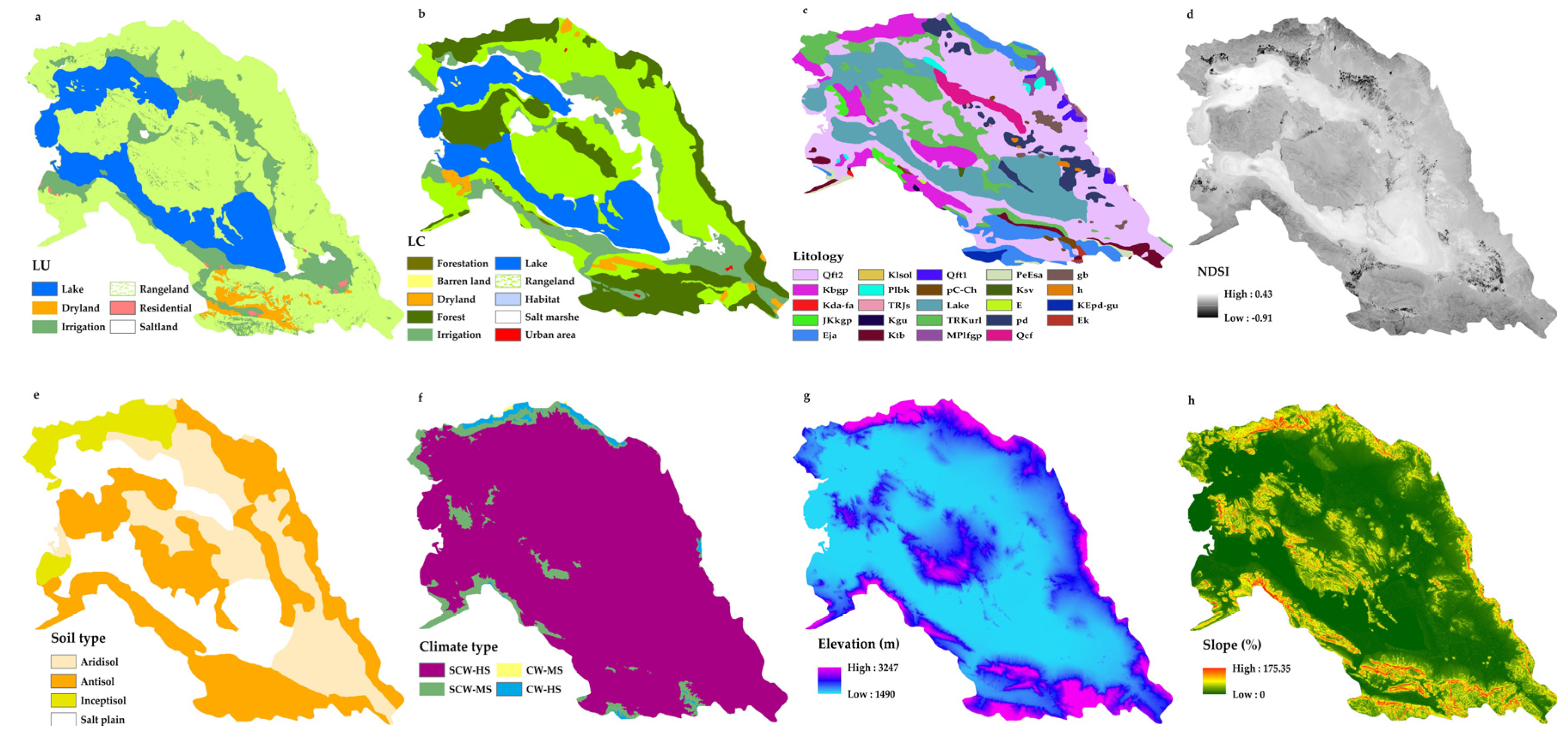
Based on past research [25,26,44,45,46,47,48,49,50,51,52], LS is considered by four different overarching criteria, including hydrometeorological (5 variables), geological (3 variables), Geomorphological (13 variables), and human-caused (6 variables) (Table 1).
Hydrometeorological criteria (e.g., a decline in groundwater level (DGWL), depth of groundwater (DTGW), flow accumulation, flow direction, and climate type) are dominant determinants of LS occurrence [25,45,47,51,52,53]. Indeed, many researchers recognize the DGWL as the leading cause of LS [25,47,51].
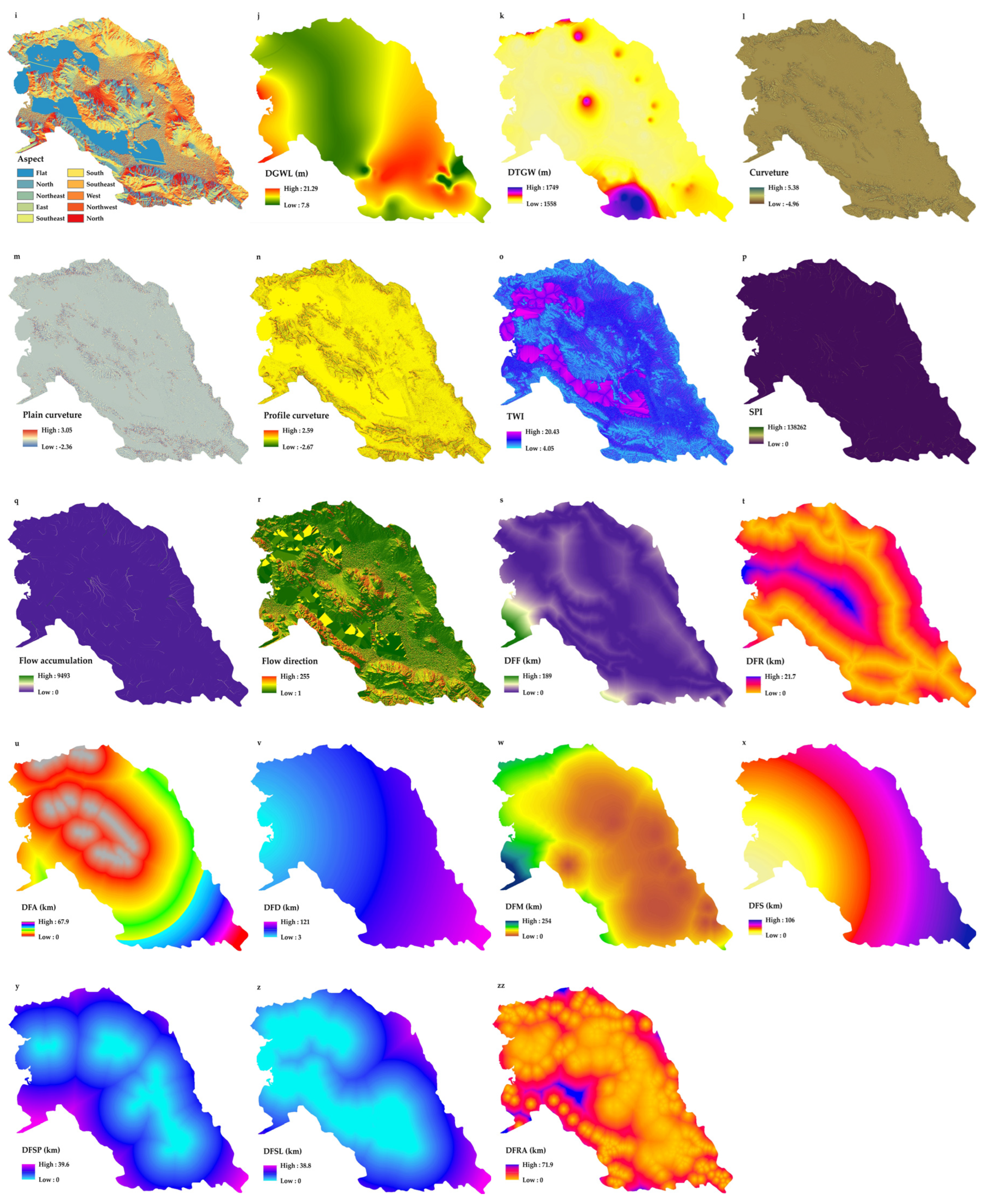
In this research, a digital elevation model (DEM) [ALOS PALSAR 12.5 × 12.5 m (https://vertex.daac.asf.alaska.edu/, accessed on 12 June 2019)] was used to obtain geomorphological variables. The geomorphological variables included elevation [54], slope [54], aspect [54], distances from anticlines and synclines [55], and profile curvature [49]). These LS-determining variables are essential in washing out and transforming saline materials from the soil to the plains of rivers, including transformation and accumulation to lowlands. Lithological units differ relative to LS because of considerable changes in compressible sediment thicknesses [26]. For example, lithology can impact the LS occurrence indirectly by affecting absorption [45]. Similarly, distance from a salt plain (DFSP; [56]) and distance from a saltwater lake (DFSL; [48]) can impact groundwater via interactions between saline and fresh waters, which can indirectly affect LS. Faults that can be the center of tectonic activities, which affect the geological structures and absorption of groundwater, can also create conditions for the accumulation of compressible sediments to impact LS [57]. Hence, the distance from the fault (DFF) is an important variable in LS. The Topographic Wetness Index (TWI) can impact groundwater via flood irrigation, surface water absorption, washing, and dissolution of solid materials in unsaturated regions [58].
Anthropogenic criteria, including land use (LU; [59]; Figure 3a), land cover (LC; [59]; Figure 3b), distance from dams (DFD; Figure 3v), distance from roads (DFR; [60]; Figure 3t), distance from mines (DFM; [61]; Figure 3w), and distance from residential areas (DFRA; [62]) also heavily impact LS occurrence. Almost 80% of LS cases are attributed to anthropogenic groundwater activities, according to Galloway and Sneed [63]. Groundwater levels drop when unconsolidated alluvial sediments occupy aquifers, which reduce pore water pressure, shifting the water’s support to the geological scaffolding beneath [3]. Many researchers have referred to human-based activities (e.g., road construction, mining, and building) and underground activities as sources of LS [64,65].
We obtained DGWL maps from the Iran Water Resources Management Company data center between 2003 and 2019 (Figure 3j). Based on the data from 124 observed wells in the Bakhtegan basin, the observed groundwater level drop ranged from 7.8 to 21.9 m (Figure 3j). The TWI (Figure 3o) was developed using SAGA GIS (Ver. 7.1.1) software. DFF (Figure 3s) was measured using Euclidean tools in Arc GIS software [66]. Lithological (Figure 3e) and fault (Figure 3s) maps were obtained from the Geological Survey of Iran (Scale = 1:100,000). Figure 3e shows a lithology map of the study area (Table S1) with 21 distinct lithological units. A map of the distance from the mine (DFM; Figure 3w), distance from the residential area (DFRA; Figure 3zz), and distance from the roads (DFR; Figure 3t) were derived using the Euclidean tools of Arc GIS. The LU and LC maps (scale = 1:500,000) were obtained from the Natural Resources and Watershed Organization of Iran.

2.2.2. Interferometric Synthetic Aperture Radar (InSAR)

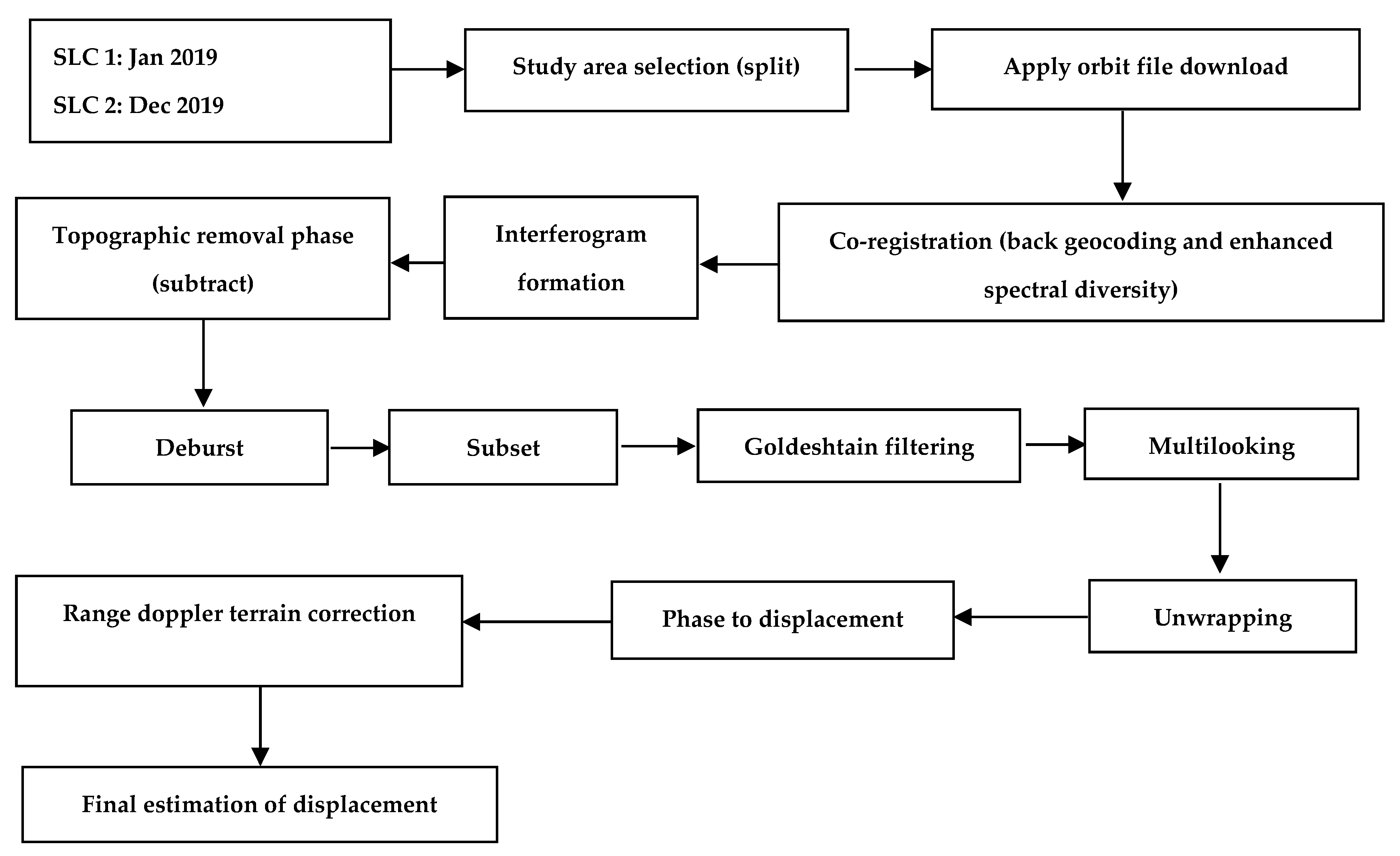
InSAR databases include surface transformation imaging and time and regional evolution along different seismic cycles for the last decade [67]. Radar interferometry extracts phase differences between two images taken from the radar sensor, the base image, and the following image. The phases of the two images can be compared after the geometric recording of the current and the prior (base) images. Information about the land surface change, elevation, and atmospheric models can be derived using the two images. The phase difference between the two images after geometric recording produces a new kind of image called an interferogram [68,69]. Each interferogram consists of displacement and other signals. Therefore, the transformation could be recognizable if the two SAR images are taken in a one-time range [70]. The radar interferometric process for extracting LS is shown in Figure 4.
In order to obtain an interferogram, the phase difference of two single look complex (SLC) images acquired after and before LS is calculated as follows (Govil and Guha, 2023):
φInt = φDef + φAtm + φCurv + φTopo + φNoise
The interferometric phase (φInt) is composed of several phase components, including the phase due to deformation (φDef), the atmospheric phase resulting from variations in atmospheric delay at the two acquisition times (φAtm), the phase component related to Earth’s curvature (φCurv), the phase component associated with topography (ΔφTopo) and the noise term due to decorrelation (φNoise) [71]. In order to obtain the contribution of deformation to the interferometric phase, it is necessary to calculate and subtract all of the relevant features from the interferogram, thus producing differential interferograms [72]. After phase unwrapping is performed, the integer phase cycles are calculated for each relative wrapped phase measurement. Finally, the radar coordinate system is geocoded into the global coordinate system. Interferograms are filtered with Goldstein filters to reduce vegetation-induced noise and to enhance signal-to-noise ratios [73].
With a minimum orbit repeat cycle of six days in both descending and ascending orbits, Sentinel-1A captured land over Iran with a resolution of 5 × 20 m (range × azimuth). For the current study, 12 images of Sentinel-1A in pass 64 (low-pass mode) collected from January to December 2019 were obtained. Radar LS values are converted from GPS measurements with some errors based on the satellite orbit accuracy. The longest wavelength component of the InSAR LS rate maps contains an error due to satellite orbital uncertainty [74]. Precise orbit ephemerides provided by Sentinel-1 quality control subsystems are used to reduce the errors associated with satellite orbits [75]. To eliminate the topographic phase’s effect and increase the accuracy of the calculations, the digital Shuttle Radar Topography Mission (SRTM) elevation model was used in the current work with a spatial resolution of 30 m for interference mapping. The atmospheric artifact is corrected using external data from the Generic Atmospheric Correction Online Service for InSAR (GACOS) [76]. As part of Sentinel-1A, the ESA provided precise orbit data so that the reference phase could be removed from differential interferograms and orbital errors could be minimized. The LS signal is readily detectable in various interferograms. The highest rate of LS was in 2019 in the southern and southwest parts of the basin and on the lake shore at the rate of 8 to 10 cm per year, respectively (Figure 5).

2.3. Most Determinant LS Susceptibility Variables

Although the indicators in this study were based on the variables used and their relative impact on the LS, additional indicators can affect the study results. Similarly, combining variables may also provide different results [77]. Therefore, an attempt was made to implement a method of selecting variables to identify the most influential variables. The contribution of the influential variables affects the models’ ability to predict LS susceptibility accurately; hence, understanding the role of the respective variable in LS susceptibility is a greatly needed area of inquiry. For example, the jackknife (cross-validation) test is a type of valuable analysis that helps to identify the relationship between LS occurrence, vulnerability, and influencing variables. Hence, this study investigated the importance of 27 variables used in modeling LS maps using the Jackknife test [43,78] in RStudio software.

2.4. LS Susceptibility Modeling and Validation Map

The effectiveness of ML models is considerably affected by data size and quality because unnecessary or unrelated variables can significantly decrease efficiency [79]. An index selection method can be implemented to identify the most critical indices and improve ML efficiency. For this purpose, the RFE was used to find and choose the most crucial combination of indices to develop LS susceptibility maps. An RFE algorithm is an optimized subset of parameters utilizing a hierarchy that identifies parameters based on the importance of RF indices (i.e., average precision decrement). The algorithm recursively makes multiple RF models. In each recursion, parameters with minor importance (identified based on mean accuracy reduction) are eliminated. Following this step, subsets of parameters with the smallest OOB error are chosen [80]. Random forest (RF) was used for this portion of the investigation. RF has been used previously and is well-accepted for these applications [81,82]. The Card package in R software was used to select the most significant indices based on five-fold cross-validation and metric precision.
The current study developed an LS susceptibility map using three ML models (CART, RF, and KNN). CART is a non-parametric method that uses input data to make prediction relations [83]. CART was used in the current study because it has shown an excellent function with internally non-linear and heterogeneous processes. This method can be used to classify the parameters, which depend on a collection of classes based on the needed level of internal homogeneity, and form a simple model for each set of parameters [84].
Breiman developed the random forest (RF) algorithm in 2001 (co-created by Cutler et al. [85]); as a classification and regression method, it can detect linear and non-linear relations between parameters for classification and regression. This method is used for assessing multiple problem cases, including the generation of a prediction law for a learning problem under observation, evaluation, and ranking of variables considering their result prediction ability. This approach includes various arbitrary decision-making trees. In this research, the RF package of R software was utilized. An RF model explicitly measures the parameter importance using the following two criteria; the average decrease in the Gini Index (GI) and an increasing percentage in RMSE [86]. In this research, we measured the importance of variables by percentage increase using RF because the GI plays a role in calculating variable importance [86]. An essential factor when using the RF model is each branch’s minimum number of leaves (notes of the decision trees). No discrete methods exist to determine the number of leaves (nodes). In the past, depending on the problem under inquiry, it has been determined based on trial and error. In this research, the minimum number of leaves is between 5 and 500, and the minimum number is determined based on trial and error.
The K-nearest neighbors (KNN) classification is a model for non-parametric classification that Wu et al. [87] named as one of the ten most prominent algorithms. Because of its simple execution and distinct operation, the method is widely used in data mining and ML observations [88]. KNN can be used to identify complex and non-linear relations among observations. The KNN classification includes the two nearest neighbor parameters (K) and the power (P) [26]. K can be assigned using source data and input variables, while P is based on the weight–distance relation and measures each data point’s (K’s) degree of similarity. The operation of the KNN models can be affected by many parameters, such as choosing different K amounts and the option of distance measurement [88].
As part of the model development procedure, validation is essential [89]. Validation is used in modeling procedures to demonstrate that the model produces accurate results [90]. Previous authors noted that ML is highly precise [84]. However, uncertainties in model predictions are inevitable, so the validity of predictions and model functionality assessment is critical. In the current study, standard deviation (STDEV), root-mean-square error (RMSE), Nash–Sutcliffe efficiency (NSE), RMSE-observations standard deviation ratio (RSR), correlation coefficient (COR), R-squared (R2), Kling–Gupta efficiency (KGE), and percentage of bias (PBIAS) [89,91,92] are provided in five packages of the R platform for the functionality and precision of the models.
S T D E V o b s = i = 1 N ( O i O ) 2
R M S E = i = 1 N ( O i P i ) 2
R S R = R M S E S T D E V o b s = [ i = 1 N ( O i P i ) 2 ] [ i = 1 N ( O i O ) 2 ]
R 2 = ( i = 1 N ( O i O i ) ( P i P ) i = 1 N ( O i O i ) 2 i = 1 N ( P i P ) ) 2
N S E = 1 i = 1 N ( O i P i ) 2 i = 1 n ( O i O i ) 2
K G E = 1 ( c c 1 ) 2 + ( α 1 ) 2 + ( β 1 ) 2
P B I A S = [ i = 1 N ( P i O i ) ( 100 ) i = 1 n ( O i ) ]

3. Results and Discussion

3.1. LS Susceptibility Prediction Maps

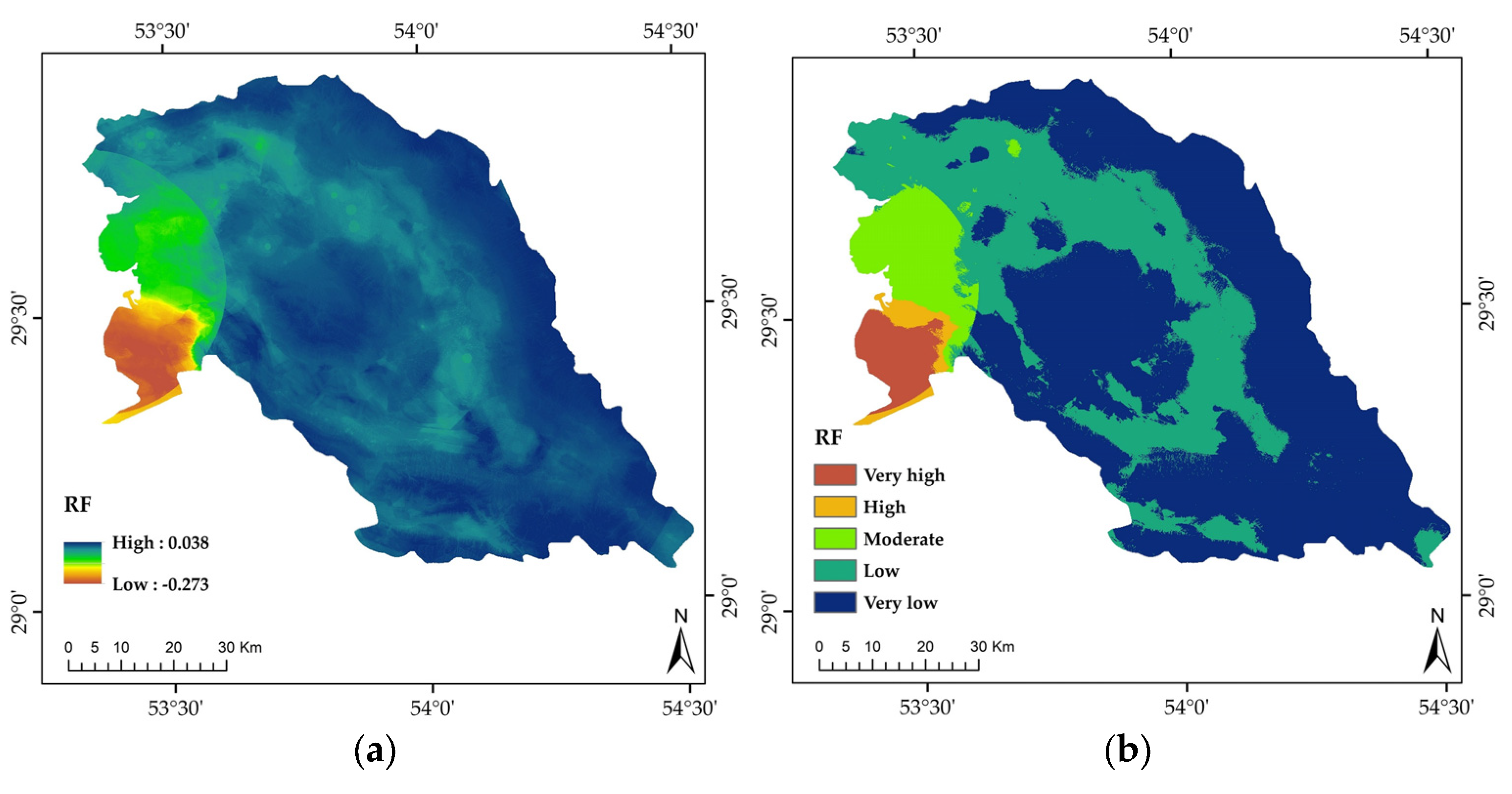
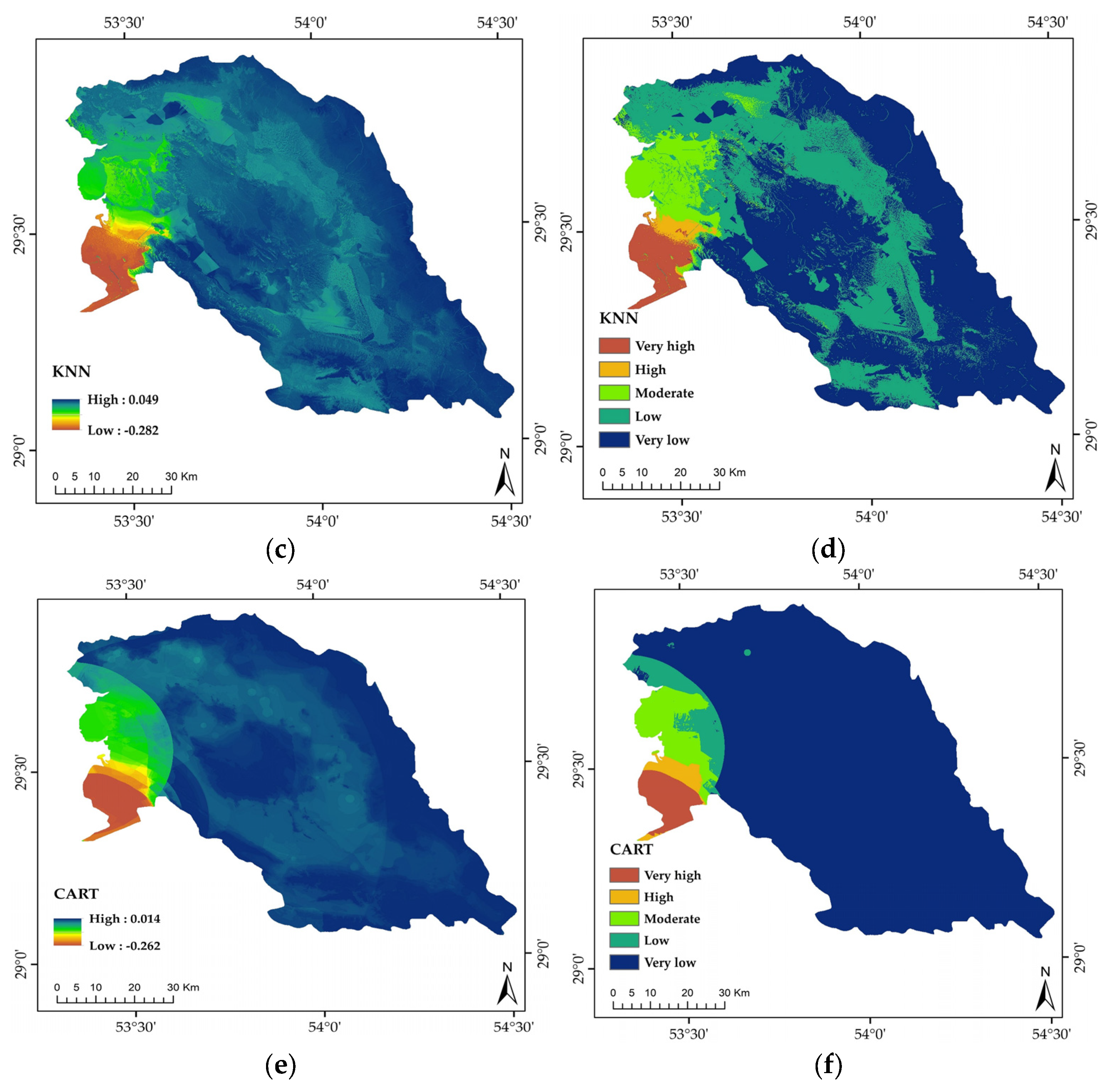
All three ML models predicted very low LS susceptibility over most of the study area (Table 2; Figure 6), with RF = 58.13%, KNN = 55.54%, and CART = 86.805 of the total land area (Table 2). For example, in the KNN model, the area of LS susceptibility classes was estimated to be 3.33, 1.08, 6.73, 33.32, and 55.54% of the region’s total area for very low to very high LS susceptibility, respectively (Table 2). Based on the results from the RF, KNN, and CART models, the highest LS susceptibility values were obtained in the western region (Figure 6).

3.2. Most Determinant LS Susceptibility Variables

For natural resource management, it is necessary to determine the most important variables (i.e., predictors) in the susceptibility to LS. Brown and Nicholls [93] highlighted that analyzing the relationships between LS and the most influential variables facilitates managers to focus on the most impactful human activities that affect LS. Subsidence-induced faulting is caused by groundwater extraction. However, there are few examples of how to determine the parameters that cause surface faults, and direct measurements are rare [94]. It has become increasingly helpful for decision-makers to use ML algorithms to gain new insights into the relationship between influential variables and LS occurrences. ML is now considered as a practical tool to improve environmental management practices in LS-prone regions [95]. To address the most determinant LS susceptibility variables, the jackknife test [43,78] was applied to evaluate the relative importance of each variable. For all three models, distance from a mine (DFM), distance from a syncline (DFS), distance from a dam (DFD), and distance from a fault (DFF) were identified as the most crucial input variables, as shown in Figure 7. The climate type, flow accumulation, and flow direction, which caused a minor increase in the modeling errors, are removed and ignored in the process (Figure 7). The type of model affects the relative importance of variables in LS modeling [96]. Thus, in one model, predictive variables may be highly important, while in another, they may not be so important. However, a consistent result across all three ML models was found in the current work. Furthermore, based on the results shown in Figure 7, the climate type, Topographic Wetness Index (TWI), flow direction, and flow accumulation indices had the most negligible impact on the occurrence of LS in the region (Figure 7).
Mining-induced catastrophic geohazards, such as LS, slowly occur around opencast mines due to the dewatering of mines [97,98]. As a result of mining activities, large areas suffer from LS, soil erosion, and waterlogging, which is detrimental to industrial and agricultural production [61,99]. He et al. [99] in China showed that the continuous operation of mines caused large-gradient LS, resulting in large-scale water accumulation in the deformation area. Similar findings have been found in the current study regarding the impact of the distance from mines (DFM) on LS. According to Loupasakis et al. [97], LS extended for 4 km around a mine in Northern Greece. Zhang et al. [70] concluded that the distribution of a salt field in China was highly correlated with the distribution of LS depression in their study area. These are similar findings to the results of the current study regarding the impact of the distance from synclines (DFS) on LS. We highlighted that the distance from dams (DFM) is one of the main factors influencing LS occurrence. Previous research showed that the construction of dams has significantly changed hydrological regimes [100] at local and regional scales, including substantially impacting LS susceptibility and occurrence [101]. For example, due to the building of dams, many river systems deliver much less sediment to flood plains [102]. A lack of adequate sediment supply leads to an uncompensated state of natural subsidence. The highest LS rate was observed downstream of the dams in central Iran [103]. The distance from faults (DFF) has been identified as the most critical variable in the occurrence of LS [56,104,105,106,107,108], because landforms can be a direct result of the activities of faults and geological structures. It is common for faults to cause the Earth’s crust to move, resulting in the subsidence of land [105]. Similarly, Bouwer [106] found that LS can occur when rigid slabs of alluvium rotate around buried faults. More LS occurs around the preexisting fault due to a weak interface within the soil body, and LS decreases as the distance to the fault increases [105]. Consistent with the work of Saro et al. [107], Shahabi et al. [108] considered the distance from laminates (faults) as the most critical variable in the occurrence of LS and stated that the DFF has a significant effect on the occurrence of LS. The present study showed that the leading cause of land LS in the study region is not due to groundwater withdrawals. Instead, the distance from dams (DFD) and the proximity to anticlines, faults, and mines (i.e., DFA, DFF, and DFM variables, respectively) are the most important identifiers of LS susceptibility [109]. However, it should not be overlooked that all the above indirectly affect local to regional groundwater processes.

3.3. Validation of LS Susceptibility Maps

The performance evaluation results of the RF, KNN, and CART models in predicting LS susceptibility indicated that all three models had relatively good results (NSE = 0.81–0.95 to 0.69–0.76 for training and validation phases, respectively; Table 3). Among the models, RF (for validation phase: STDEV = 0.04, RMSE = 0.02, NSE = 0.76, COR = 0.88, and KGE = 0.78) achieved the highest predictive capability, followed by CART (for validation phase: STDEV = 0.04, RMSE = 0.03, NSE = 0.71, COR = 0.85, and KGE = 0.75) (Table 3). Previous studies have shown that RF models perform better than CART models, which is consistent with this result [110,111,112]. Since none of these previous studies simultaneously applied these three ML models (RF, CART, and KNN) to LS prediction, a direct comparison of our results with theirs is difficult. However, a few studies have examined the performance of RF, CART, and KNN in other natural resources disciplines, including flood susceptibility [113], land-use and land-cover change [114], and ecological modeling [80], which showed similar trends relative to the ML models used in the current investigation and using the same (or similar) data set. The present work showed that a decision tree using several classification algorithms (i.e., RF) yields more reliable results than a single classification algorithm [115]. Because single models sometimes have bias, variance, and classification errors, in decision tree models using multiple single models (such as RF), the classification performance increases, and their variance and errors decrease [110]. In the present study, it was found that fitting multiple trees in the RF model was capable of overcoming one of the greatest disadvantages of single decision tree models, that is, low predictive performance [110,116,117]. According to Pham et al. [118], when surface and subsurface processes are complex, it is necessary to use more non-linearity rules to model geohazards (e.g., LS) in heterogeneous terrains, and models with greater flexibility perform better. Importantly, all three ML models demonstrated good performance, thus highlighting their overall capabilities in modeling LS using ML techniques, similar to past research [110]. Based on the map generated by the RF algorithm (Figure 6), the highest probability of LS susceptibility was found at distances less than 18 km from synclines, 6 to 13 km from anticlines, 23 km from dams, and distances less than 20 to more than 144 km from mines.

3.4. Study Implications and Future Directions

In Iran, around 50% of the plains lack water, and there is likely to be continued pumping of water (legal or unauthorized), which could lead to LS [49]. Prevention of or reduction in LS susceptibility can be aided by robust, accurate, and meaningful spatial modeling. The results of the current research show that land subsidence in the study area dramatically contributes to the subsequent conversion of valuable ecological land into degraded non-producing land. This finding is consistent with the LS trends in other parts of Iran from the end of the last century to the beginning of the 21st century [24,119,120]. This awareness has increased as water agencies have increasingly released reports identifying the cumulative impacts of subsidence on significant infrastructure, resulting in hundreds of millions of dollars of damage. For example, the highest rate of LS was in 2019 at the rate of 8 to 10 cm per year in the southern and southwest parts of the study area and the lake shore (Figure 5). The findings of the current investigation strongly support the need to include addressing subsidence as part of Iran’s groundwater management requirements. In addition, while beyond the scope of the present study, future research should involve using the methods developed in the current work to create a framework to estimate LS with various techniques and apply it to a series of validation studies in different parts of Iran. This would facilitate the building of a set of comparable case studies that may allow the aggregation of environmental effects of LS in various parts of the country and the world. Finally, LS processes are dynamic, requiring the continuous updating of susceptibility zoning maps, such as the innovative processes presented here. With the aid of advanced InSAR analysis techniques that utilize newly acquired data, as well as GNSS stations, it will be possible to generate updated LS susceptibility and rate maps.

4. Conclusions

Environmental destruction is a consequence of land subsidence (LS). Hence, the identification, assessment, mapping, modeling, and management of LS are essential. In this study, we first estimated the exact amount of LS using an interferometric synthetic aperture radar (InSAR) technique. Then, the variables that affect LS susceptibility in the Bakhtegan basin were prioritized using three ML models (i.e., RF, KNN, and CART). The results showed that the RF model had the highest conformity and correlation coefficient among the models to predict the LS phenomenon. Based on the validation results of the models, the RF model had excellent predictive power and can be used to analyze geographical and environmental variables and plot the susceptibility of LS. The present study showed that the determinants and subsequent susceptibility of LS in the region of study are most highly related to the distance from a dam (DFD), distance from an anticline (DFA), distance from a fault (DFF), and distance from a mine (DFM). It was also shown that InSAR is a powerful tool for measuring LS in the drylands of Iran. In addition, the RF algorithm was shown to be an appropriate model to assist land managers, conservation authorities, natural resources stakeholders, and policy-makers in improving LS preventative practices and decision-making. While the ML methods used in this study have been previously applied in various fields, they are novel in the context of LS susceptibility prediction. The methodology presented in this study can serve as a template for others wishing to advance predictive confidence in LS susceptibility in other regions globally.

Supplementary Materials

The following supporting information can be downloaded at: https://www.mdpi.com/article/10.3390/land12040843/s1, Table S1: Descriptions of the lithology of the Bakhtegan basin. Reference [121] are cited in the Supplementary Materials.

Author Contributions

Conceptualization, H.G., A.N.S. and S.K.S.; methodology, H.G., A.N.S. and S.K.S.; software, H.G., M.S.M. and A.B.; validation, H.G.; formal analysis, H.G.; investigation, H.G. and S.M.M.S.; resources, A.N.S. and S.K.S.; writing—original draft preparation, H.G. and M.S.M.; writing—review and editing, J.A.H. and S.M.M.S.; visualization, H.G. and S.M.M.S.; supervision, A.N.S. and S.K.S.; funding acquisition, S.M.M.S. All authors have read and agreed to the published version of the manuscript.

Funding

This research received no external funding.

Data Availability Statement

The data that support the findings of this study are available from the first and second authors, upon reasonable request.

Acknowledgments

We are very thankful to Azade Deljouei (University of Florida) and Fardin Moradi (Razi University) for the constructive comments and valuable suggestions that helped us to improve the overall quality of our manuscript.

Conflicts of Interest

The authors declare no conflict of interest.

References

  1. Shi, X.; Jiang, S.; Xu, H.; Jiang, F.; He, Z.; Wu, J. The effects of artificial recharge of groundwater on controlling land subsidence and its influence on groundwater quality and aquifer energy storage in Shanghai, China. Environ. Earth Sci. 2016, 75, 195. [Google Scholar] [CrossRef]
  2. Batubara, B.; Kooy, M.; Zwarteveen, M. Politicising land subsidence in Jakarta: How land subsidence is the outcome of uneven sociospatial and socionatural processes of capitalist urbanization. Geoforum 2023, 139, 103689. [Google Scholar] [CrossRef]
  3. Li, Z.; Chen, Q.; Xue, Y.; Qiu, D.; Chen, H.; Kong, F.; Liu, Q. Numerical investigation of processes, features, and control of land subsidence caused by groundwater extraction and coal mining: A case study from eastern China. Environ. Earth Sci. 2023, 82, 82. [Google Scholar] [CrossRef]
  4. Jiang, H.; Zhang, J.; Liu, Y.; Li, J.; Fang, Z.N. Does flooding get worse with subsiding land? Investigating the impacts of land subsidence on flood inundation from Hurricane Harvey. Sci. Total Environ. 2023, 865, 161072. [Google Scholar] [CrossRef] [PubMed]
  5. Kadiyan, N.; Chatterjee, R.; Pranjal, P.; Agrawal, P.; Jain, S.; Angurala, M.; Biyani, A.; Sati, M.; Kumar, D.; Bhardwaj, A. Assessment of groundwater depletion–induced land subsidence and characterisation of damaging cracks on houses: A case study in Mohali-Chandigarh area, India. Bull. Eng. Geol. Environ. 2021, 80, 3217–3231. [Google Scholar] [CrossRef]
  6. Wang, C.-M. Securing the subterranean volumes: Geometrics, land subsidence and the materialities of things. Environ. Plan. D Soc. Space 2021, 39, 218–236. [Google Scholar] [CrossRef]
  7. Johnston, J.; Cassalho, F.; Miesse, T.; Ferreira, C.M. Projecting the effects of land subsidence and sea level rise on storm surge flooding in Coastal North Carolina. Sci. Rep. 2021, 11, 21679. [Google Scholar] [CrossRef]
  8. Wang, Z.; Liu, Y.; Zhang, Y.; Liu, Y.; Wang, B.; Zhang, G. Spatially Varying Relationships between Land Subsidence and Urbanization: A Case Study in Wuhan, China. Remote Sens. 2022, 14, 291. [Google Scholar] [CrossRef]
  9. El Kamali, M.; Papoutsis, I.; Loupasakis, C.; Abuelgasim, A.; Omari, K.; Kontoes, C. Monitoring of land surface subsidence using persistent scatterer interferometry techniques and ground truth data in arid and semi-arid regions, the case of Remah, UAE. Sci. Total Environ. 2021, 776, 145946. [Google Scholar] [CrossRef]
  10. Pan, Y.; Ding, H.; Li, J.; Shum, C.K.; Mallick, R.; Jiao, J.; Zhang, Y. Transient hydrology-induced elastic deformation and land subsidence in Australia constrained by contemporary geodetic measurements. Earth Planet. Sci. Lett. 2022, 588, 117556. [Google Scholar] [CrossRef]
  11. Charpentier, A.; James, M.; Ali, H. Predicting drought and subsidence risks in France. Nat. Hazards Earth Syst. Sci. 2022, 22, 2401–2418. [Google Scholar] [CrossRef]
  12. Cenni, N.; Fiaschi, S.; Fabris, M. Monitoring of land subsidence in the po river delta (Northern Italy) using geodetic networks. Remote Sens. 2021, 13, 1488. [Google Scholar] [CrossRef]
  13. Przyłucka, M.; Kowalski, Z.; Perski, Z. Twenty years of coal mining-induced subsidence in the Upper Silesia in Poland identified using InSAR. Int. J. Coal Sci. Technol. 2022, 9, 86. [Google Scholar] [CrossRef]
  14. Imamoglu, M.; Balik Sanli, F.; Cakir, Z.; Kahraman, F. Rapid ground subsidence in the Küçük Menderes Graben (W. Turkey) captured by Sentinel-1 SAR data. Environ. Earth Sci. 2022, 81, 221. [Google Scholar] [CrossRef]
  15. Ellis, J.; Knight, J.E.; White, J.T.; Sneed, M.; Hughes, J.D.; Ramage, J.K.; Braun, C.L.; Teeple, A.; Foster, L.K.; Rendon, S.H.; et al. Hydrogeology, Land-Surface Subsidence, and Documentation of the Gulf Coast Land Subsidence and Groundwater-Flow (GULF) Model, Southeast Texas, 1897–2018 (No. 1877); US Geological Survey: Reston, VA, USA, 2023. [Google Scholar]
  16. Fernández-Torres, E.A.; Cabral-Cano, E.; Novelo-Casanova, D.A.; Solano-Rojas, D.; Havazli, E.; Salazar-Tlaczani, L. Risk assessment of land subsidence and associated faulting in Mexico City using InSAR. Nat. Hazards 2022, 112, 37–55. [Google Scholar] [CrossRef]
  17. Solorza, R.; Carignano, C.; Cioccale, M.; Notarnicola, C. Ground Surface Subsidence in Córdoba, Argentina, revealed by multitemporal SAR interferometry. In Proceedings of the 2022 IEEE Biennial Congress of Argentina (ARGENCON), San Juan, Argentina, 7–9 September 2022; pp. 1–7. [Google Scholar]
  18. Nishi, K.; Kawai, M.; Cahyono, B.E.; Waqar, M.M.; Nishi, K.; Tetuko Sri Sumantyo, J. Consecutive DInSAR and well based on the law of material conservation between land surface pressure and ground water to observe land subsidence. Geocarto Int. 2023, 38, 2159069. [Google Scholar] [CrossRef]
  19. Lei, K.; Ma, F.; Chen, B.; Luo, Y.; Cui, W.; Zhao, L.; Wang, X.; Sun, A. Effects of South-to-North Water Diversion Project on groundwater and land subsidence in Beijing, China. Bull. Eng. Geology Environ. 2023, 82, 18. [Google Scholar] [CrossRef]
  20. Sittiwong, A.; BALZ, T. Study of Land Subsidence by INSAR Time Series of ALOS-2, Sentinel-1 and GNSS CORS Stations in Chaopraya Basin, Samutprakan, Thailand. Ph.D. Dissertation, Burapha University, Chon Buri, Thailand, 2022. [Google Scholar]
  21. Hayati, N.; Widodo, A.; Kurniawan, A.; Sanjiwani, I.D.M.A.; Darminto, M.R.; Yudha, I.S.; Sumantyo, J.T.S. Small baselines techniques of time series InSAR to monitor and predict land subsidence causing flood vulnerability in Sidoarjo, Indonesia. Geomat. Nat. Hazards Risk 2022, 13, 2124–2150. [Google Scholar] [CrossRef]
  22. Raju, A.; Nanda, R.; Singh, A.; Malik, K. Multi-temporal analysis of groundwater depletion-induced land subsidence in Central Ganga Alluvial plain, Northern India. Geocarto Int. 2022, 37, 11732–11755. [Google Scholar] [CrossRef]
  23. Shahbazi, S.; Mousavi, Z.; Rezaei, A. Constraints on the hydrogeological properties and land subsidence through GNSS and InSAR measurements and well data in Salmas plain, northwest of Urmia Lake, Iran. Hydrogeol. J. 2022, 30, 533–555. [Google Scholar] [CrossRef]
  24. Sorkhabi, O.M.; Kurdpour, I.; Sarteshnizi, R.E. Land subsidence and groundwater storage investigation with multi sensor and extended Kalman filter. Groundw. Sustain. Develop. 2022, 19, 100859. [Google Scholar] [CrossRef]
  25. Kumar, H.; Syed, T.H.; Amelung, F.; Agrawal, R.; Venkatesh, A. Space-time evolution of land subsidence in the National Capital Region of India using ALOS-1 and Sentinel-1 SAR data: Evidence for groundwater overexploitation. J. Hydrol. 2022, 605, 127329. [Google Scholar] [CrossRef]
  26. Rahmati, O.; Falah, F.; Naghibi, S.A.; Biggs, T.; Soltani, M.; Deo, R.C.; Cerdà, A.; Mohammadi, F.; Bui, D.T. Land subsidence modelling using tree-based machine learning algorithms. Sci. Total Environ. 2019, 672, 239–252. [Google Scholar] [CrossRef] [PubMed]
  27. Liu, X.; Ma, C.; Ling, H.; Yan, W.; Zhang, H.; Jiang, X. Analysis of land subsidence caused by hydrodynamic force in Loess Hilly and gully region based on SBAS-InSAR. PLoS ONE 2023, 18, e0279832. [Google Scholar] [CrossRef]
  28. Strozzi, T.; Wegmuller, U.; Tosi, L.; Bitelli, G.; Spreckels, V. Land subsidence monitoring with differential SAR interferometry. Photogramm. Eng. Remote Sens. 2001, 67, 1261–1270. [Google Scholar]
  29. Bai, L.; Jiang, L.; Wang, H.; Sun, Q. Spatiotemporal characterization of land subsidence and uplift (2009–2010) over wuhan in central china revealed by terrasar-X insar analysis. Remote Sens. 2016, 8, 350. [Google Scholar] [CrossRef] [Green Version]
  30. Galloway, D.L.; Hoffmann, J. The application of satellite differential SAR interferometry-derived ground displacements in hydrogeology. Hydrogeol. J. 2007, 15, 133–154. [Google Scholar] [CrossRef] [Green Version]
  31. Galloway, D.L.; Hudnut, K.W.; Ingebritsen, S.; Phillips, S.P.; Peltzer, G.; Rogez, F.; Rosen, P. Detection of aquifer system compaction and land subsidence using interferometric synthetic aperture radar, Antelope Valley, Mojave Desert, California. Water Resour. Res. 1998, 34, 2573–2585. [Google Scholar] [CrossRef]
  32. Othman, A.; Sultan, M.; Becker, R.; Alsefry, S.; Alharbi, T.; Gebremichael, E.; Alharbi, H.; Abdelmohsen, K. Use of geophysical and remote sensing data for assessment of aquifer depletion and related land deformation. Surv. Geophys. 2018, 39, 543–566. [Google Scholar] [CrossRef] [Green Version]
  33. Golian, M.; Saffarzadeh, A.; Katibeh, H.; Mahdad, M.; Saadat, H.; Khazaei, M.; Sametzadeh, E.; Ahmadi, A.; Sharifi Teshnizi, E.; Samadi Darafshani, M. Consequences of groundwater overexploitation on land subsidence in Fars Province of Iran and its mitigation management programme. Water Environ. J. 2021, 35, 975–985. [Google Scholar] [CrossRef]
  34. Nalbandan, R.B.; Delavar, M.; Abbasi, H.; Zaghiyan, M.R. Model-based water footprint accounting framework to evaluate new water management policies. J. Clean. Prod. 2023, 382, 135220. [Google Scholar] [CrossRef]
  35. Bagheri, F.; Hajinejad, A.; Abdi, N. 5 Heritage Conservation for Tourism Development: Identifying the Challenges in Developing Countries–The Case of Iran. In Tourism Planning And Development In The Middle Eastl; CABI: Wallingford, UK, 2023; p. 61. [Google Scholar]
  36. Amirkhani, M.; Zarei, H.; Radmanesh, F.; Pande, S. An operational sociohydrological model to understand the feedbacks between community sensitivity and environmental flows for an endorheic lake basin, lake Bakhtegan, Iran. J. Hydrol. 2022, 605, 127375. [Google Scholar] [CrossRef]
  37. Mozafari, M.; Hosseini, Z.; Fijani, E.; Eskandari, R.; Siahpoush, S.; Ghader, F. Effects of climate change and human activity on lake drying in Bakhtegan Basin, southwest Iran. Sustain. Water Resour. Manag. 2022, 8, 109. [Google Scholar] [CrossRef]
  38. Noori, R.; Maghrebi, M.; Mirchi, A.; Tang, Q.; Bhattarai, R.; Sadegh, M.; Noury, M.; Torabi Haghighi, A.; Kløve, B.; Madani, K. Anthropogenic depletion of Iran’s aquifers. Proc. Natl. Acad. Sci. USA 2021, 118, e2024221118. [Google Scholar] [CrossRef]
  39. Hassanshahi, H.; Dastoor, J. Reconnaissance soil survey of Neyriz basin (Fars Province). Soil Water Res. Inst. 1995, 12, 1–10. [Google Scholar]
  40. Sheikholeslami, M.; Pique, A.; Mobayen, P.; Sabzehei, M.; Bellon, H.; Emami, M.H. Tectono-metamorphic evolution of the Neyriz metamorphic complex, Quri-kor-e-sefid area (Sanandaj-Sirjan Zone, SW Iran). J. Asian Earth Sci. 2008, 31, 504–521. [Google Scholar] [CrossRef]
  41. Panahi, M.; Khosravi, K.; Golkarian, A.; Roostaei, M.; Barzegar, R.; Omidvar, E.; Rezaie, F.; Saco, P.M.; Sharifi, A.; Jun, C. A country-wide assessment of Iran’s land subsidence susceptibility using satellite-based InSAR and machine learning. Geocarto Int. 2022, 37, 14065–14087. [Google Scholar] [CrossRef]
  42. Arjasakusuma, S.; Kusuma, S.; Rafif, R.; Saringatin, S.; Wicaksono, P. Time-series Cross-orbit Sentinel-1 Synthetic-Aperture Radar (SAR) Data for Mapping Paddy Extent: Case Study of Magelang District, Central Java. In Proceedings of the IOP Conference Series: Earth and Environmental Science, Yogyakarta, Indonesia, 4–5 November 2020; p. 012053. [Google Scholar]
  43. Abolhasani, A.; Zehtabian, G.; Khosravi, H.; Rahmati, O.; Alamdarloo, E.H.; D’Odorico, P. A new conceptual framework for spatial predictive modelling of land degradation in a semiarid area. Land Degrad. Develop. 2022, 33, 3358–3374. [Google Scholar] [CrossRef]
  44. Abdollahi, S.; Pourghasemi, H.R.; Ghanbarian, G.A.; Safaeian, R. Prioritization of effective factors in the occurrence of land subsidence and its susceptibility mapping using an SVM model and their different kernel functions. Bull. Eng. Geol. Environ. 2019, 78, 4017–4034. [Google Scholar] [CrossRef]
  45. Arabameri, A.; Saha, S.; Roy, J.; Tiefenbacher, J.P.; Cerda, A.; Biggs, T.; Pradhan, B.; Ngo, P.T.T.; Collins, A.L. A novel ensemble computational intelligence approach for the spatial prediction of land subsidence susceptibility. Sci. Total Environ. 2020, 726, 138595. [Google Scholar] [CrossRef]
  46. Bagheri-Gavkosh, M.; Hosseini, S.M.; Ataie-Ashtiani, B.; Sohani, Y.; Ebrahimian, H.; Morovat, F.; Ashrafi, S. Land subsidence: A global challenge. Sci. Total Environ. 2021, 778, 146193. [Google Scholar] [CrossRef] [PubMed]
  47. Tao, W.; Jia, H.; Kang, M.; Liu, Y. Application of PS-InSAR method based on time series combination in surface deformation monitoring of Xiongxian county and its surrounding areas. Bull. Surv. Mapp. 2023, 101–106. [Google Scholar]
  48. Jin, B.; Yin, K.; Li, Q.; Gui, L.; Yang, T.; Zhao, B.; Guo, B.; Zeng, T.; Ma, Z. Susceptibility Analysis of Land Subsidence along the Transmission Line in the Salt Lake Area Based on Remote Sensing Interpretation. Remote Sens. 2022, 14, 3229. [Google Scholar] [CrossRef]
  49. Feng, Z.; Li, L.; Sun, Z.; Yu, Z.; Song, X. Study on the deformation mechanism of the upper overburden during the dewatering of confined water. In Advances in Civil Engineering and Environmental Engineering; CRC Press: Boca Raton, FL, USA, 2023; Volume 2, pp. 192–197. [Google Scholar]
  50. Bramanto, B.; Gumilar, I.; Sidiq, T.P.; Rahmawan, Y.A.; Abidin, H.Z. Geodetic evidence of land subsidence in Cirebon, Indonesia. Remote Sens. Appl. Soc. Environ. 2023, 30, 100933. [Google Scholar] [CrossRef]
  51. Sudarmanto, A.; Khalif, M.A.; Huda, A.K. Detection of building slope and land subsidence using ultrasonic HC-SR04 sensors based Arduino Uno R3 and Blynk. In AIP Conference Proceedings; AIP Publishing LLC: Surakarta, Indonesia, 2023; Volume 2540, p. 100004. [Google Scholar]
  52. Zeraatkar, Z.; Siuki, A.K.; Shahidi, A. Delineation of the Areas with Potential Land Subsidence Using the Analytic Network Process (Case Study: Birjand Aquifer, Iran). Geogr. Nat. Resour. 2021, 42, 290–295. [Google Scholar] [CrossRef]
  53. Zhang, Y.; Yang, Y.; Zhang, J.; Wang, Y. Sensitivity study of multi-field information maps of typical landslides in mining areas based on transfer learning. Front. Earth Sci. 2023, 11, 1105985. [Google Scholar] [CrossRef]
  54. Eghrari, Z.; Delavar, M.R.; Zare, M.; Beitollahi, A.; Nazari, B. Land Subsidence Suspectibility Mapping Using Machine Learning Algorithms. ISPRS Ann. Photogramm. Remote Sens. Spat. Inf. Sci. 2023, 4, 129–136. [Google Scholar] [CrossRef]
  55. Tomás, R.; Márquez, Y.; Lopez-Sanchez, J.M.; Delgado, J.; Blanco, P.; Mallorquí, J.; Navarrete, D.; Duque, S. Relationship between piezometric level and ground deformations measured by means of DInSAR in the Vega Media of the Segura River (Spain). In Proceedings of the Fringe 2005 Workshop, Frascati, Italy, 28 November–2 December 2005. [Google Scholar]
  56. Pourghasemi, H.R.; Saravi, M.M. Land-subsidence spatial modeling using the random forest data-mining technique. In Spatial Modeling in GIS and R for Earth and Environmental Sciences; Elsevier: Amsterdam, The Netherlands, 2019; pp. 147–159. [Google Scholar]
  57. Garcıa-Palomo, A.; Macıas, J.; Garduño, V. Miocene to recent structural evolution of the Nevado de Toluca volcano region, Central Mexico. Tectonophysics 2000, 318, 281–302. [Google Scholar] [CrossRef]
  58. Foster, S.; Chilton, J.; Moencg, M.; Cardy, F.; Schiffler, M. Groundwater in Rural Development: Facing the Challenges of Supply and Resource Sustainability; The World Bank: Washington, DC, USA, 2000. [Google Scholar]
  59. Shihran, R.S.; Gumilar, I.; Sidiq, T.P.; Bramanto, B. A Preliminary Result of Land subsidence Monitoring by Using Low-Cost GNSS in Bandung Basin. IOP Conf.Series Earth Environ. Sci. 2023, 1127, 012001. [Google Scholar] [CrossRef]
  60. Tangdamrongsub, N.; Han, S.-C.; Jasinski, M.F.; Šprlák, M. Quantifying water storage change and land subsidence induced by reservoir impoundment using GRACE, Landsat, and GPS data. Remote Sens. Environ. 2019, 233, 111385. [Google Scholar] [CrossRef]
  61. Hu, Z.; Xu, X.; Zhao, Y. Dynamic monitoring of land subsidence in mining area from multi-source remote-sensing data–a case study at Yanzhou, China. Int. J. Remote Sens. 2012, 33, 5528–5545. [Google Scholar] [CrossRef]
  62. Karanam, V.; Motagh, M.; Garg, S.; Jain, K. Multi-sensor remote sensing analysis of coal fire induced land subsidence in Jharia Coalfields, Jharkhand, India. Int. J.Appl. Earth Obs. Geoinf. 2021, 102, 102439. [Google Scholar] [CrossRef]
  63. Galloway, D.L.; Sneed, M. Analysis and simulation of regional subsidence accompanying groundwater abstraction and compaction of susceptible aquifer systems in the USA. Boletín Soc. Geológica Mex. 2013, 65, 123–136. [Google Scholar] [CrossRef]
  64. Huang, Z.; Yu, F. InSAR-derived surface deformation of Chaoshan Plain, China: Exploring the role of human activities in the evolution of coastal landscapes. Geomorphology 2023, 426, 108606. [Google Scholar] [CrossRef]
  65. Spacagna, R.L.; Modoni, G. Gis-based study of land subsidence in the city of Bologna. In Mechatronics for Cultural Heritage and Civil Engineering; Springer: Cham, Swizerland, 2018; pp. 235–256. [Google Scholar]
  66. El Jazouli, A.; Barakat, A.; Khellouk, R. GIS-multicriteria evaluation using AHP for landslide susceptibility mapping in Oum Er Rbia high basin (Morocco). Geoenviron. Disasters 2019, 6, 3. [Google Scholar] [CrossRef]
  67. Zhao, D.; Qu, C.; Chen, H.; Shan, X.; Song, X.; Gong, W. Tectonic and geometric control on fault kinematics of the 2021 Mw7. 3 Maduo (China) earthquake inferred from interseismic, coseismic, and postseismic InSAR observations. Geophys. Res. Lett. 2021, 48, e2021GL095417. [Google Scholar] [CrossRef]
  68. Just, D.; Bamler, R. Phase statistics of interferograms with applications to synthetic aperture radar. Appl. Opt. 1994, 33, 4361–4368. [Google Scholar] [CrossRef]
  69. Silva, B.; Sousa, J.J.; Lazecky, M.; Cunha, A. Deformation Fringes Detection in SAR interferograms Using Deep Learning. Procedia Comput. Sci. 2022, 196, 151–158. [Google Scholar] [CrossRef]
  70. Zhang, B.; Wang, R.; Deng, Y.; Ma, P.; Lin, H.; Wang, J. Mapping the Yellow River Delta land subsidence with multitemporal SAR interferometry by exploiting both persistent and distributed scatterers. ISPRS J. Photogramm. Remote Sens. 2019, 148, 157–173. [Google Scholar] [CrossRef]
  71. Govil, H.; Guha, S. Underground mine deformation monitoring using Synthetic Aperture Radar technique: A case study of Rajgamar coal mine of Korba Chhattisgarh, India. J. Appl. Geophys. 2023, 209, 104899. [Google Scholar]
  72. Welikanna, D.R.; Jin, S. Investigating ground deformation due to a series of collapse earthquakes by means of the PS-InSAR technique and Sentinel 1 data in Kandy, Sri Lanka. J. Appl. Remote Sens. 2023, 17, 014507. [Google Scholar] [CrossRef]
  73. Goldstein, R.M.; Werner, C.L. Radar interferogram filtering for geophysical applications. Geophys. Res. Lett. 1998, 25, 4035–4038. [Google Scholar] [CrossRef] [Green Version]
  74. Hanssen, R.F. Radar Interferometry: Data Interpretation and Error Analysis; Springer Science & Business Media: Berlin/Heidelberg, Germany, 2001; Volume 2. [Google Scholar]
  75. Lee, J.Y.; Jung, S.W.; Hong, S.H. Mapping lava flow from the Kilauea eruption of 2018 in the east rift zone using space-based synthetic aperture radar. GIScience Remote Sens. 2023, 60, 2176275. [Google Scholar] [CrossRef]
  76. Yu, C.; Li, Z.; Penna, N.T.; Crippa, P. Generic atmospheric correction model for interferometric synthetic aperture radar observations. J. Geophys. Res. Solid Earth 2018, 123, 9202–9222. [Google Scholar] [CrossRef]
  77. Mousavi, S.M.; Shamsai, A.; Naggar, M.H.E.; Khamehchian, M. A GPS-based monitoring program of land subsidence due to groundwater withdrawal in Iran. Can. J. Civ. Eng. 2001, 28, 452–464. [Google Scholar] [CrossRef]
  78. Rodgers, J.L. The bootstrap, the jackknife, and the randomization test: A sampling taxonomy. Multivar. Behav. Res. 1999, 34, 441–456. [Google Scholar] [CrossRef]
  79. Moradi, F.; Darvishsefat, A.A.; Pourrahmati, M.R.; Deljouei, A.; Borz, S.A. Estimating Aboveground Biomass in Dense Hyrcanian Forests by the Use of Sentinel-2 Data. Forests 2022, 13, 104. [Google Scholar] [CrossRef]
  80. Islam, M.M.; Kashem, M.A.; Uddin, J. Fish survival prediction in an aquatic environment using random forest model. Int. J. Artif. Intell. ISSN 2021, 2252, 8938. [Google Scholar] [CrossRef]
  81. Bayrak, C.S.; Stein, D.; Jain, A.; Chaudhary, K.; Nadkarni, G.N.; Van Vleck, T.T.; Puel, A.; Boisson-Dupuis, S.; Okada, S.; Stenson, P.D. Identification of discriminative gene-level and protein-level features associated with pathogenic gain-of-function and loss-of-function variants. Am. J. Hum. Genet. 2021, 108, 2301–2318. [Google Scholar] [CrossRef]
  82. Rado, O.; Ali, N.; Sani, H.M.; Idris, A.; Neagu, D. Performance analysis of feature selection methods for classification of healthcare datasets. In Proceedings of the Intelligent Computing: Proceedings of the 2019 Computing Conference, London, UK, 16–17 July 2019; Volume 1, pp. 929–938. [Google Scholar]
  83. Gordon, L. Using classification and regression trees (CART) in SAS® enterprise miner TM for applications in public health. In Proceedings of the SAS Global Forum, San Francisco, CA, USA, 28 April–1 May 2013; p. 2013. [Google Scholar]
  84. Choubin, B.; Moradi, E.; Golshan, M.; Adamowski, J.; Sajedi-Hosseini, F.; Mosavi, A. An ensemble prediction of flood susceptibility using multivariate discriminant analysis, classification and regression trees, and support vector machines. Sci. Total Environ. 2019, 651, 2087–2096. [Google Scholar] [CrossRef]
  85. Cutler, D.R.; Edwards Jr, T.C.; Beard, K.H.; Cutler, A.; Hess, K.T.; Gibson, J.; Lawler, J.J. Random forests for classification in ecology. Ecology 2007, 88, 2783–2792. [Google Scholar] [CrossRef] [PubMed]
  86. Wu, C.W.; Li, C.S.; Wang, W.; Liang, J.H.; Yan, G.H. Application of an improved support vector machine algorithm in the diagnosis of breast cancer. Comput. Eng. Sci. 2023, 39, 562. [Google Scholar]
  87. Wu, X.; Kumar, V.; Ross Quinlan, J.; Ghosh, J.; Yang, Q.; Motoda, H.; McLachlan, G.J.; Ng, A.; Liu, B.; Yu, P.S. Top 10 algorithms in data mining. Knowl. Inf. Syst. 2008, 14, 1–37. [Google Scholar] [CrossRef] [Green Version]
  88. Zhang, S.; Li, X.; Zong, M.; Zhu, X.; Wang, R. Efficient kNN classification with different numbers of nearest neighbors. IEEE Trans. Neural Netw. Learn. Syst. 2017, 29, 1774–1785. [Google Scholar] [CrossRef] [PubMed]
  89. Nazari, M.; Chaichi, M.; Kamel, H.; Grismer, M.; Sadeghi, S.M.M. Evaluation of estimation methods for monthly reference evapotranspiration in arid climates. Arid. Ecosyst. 2020, 10, 329–336. [Google Scholar] [CrossRef]
  90. Abdi, E.; Mariv, H.S.; Mashayekhi, Z.; Deljouei, A.; Rahbarisisakht, S. Seasonal Variation of GPS Accuracy and Precision in Forest Road Mapping. Bull. Transilv. Uni. Bras. Ser. II For. Wood Indus. Agric. Food Eng. 2022, 15, 1–12. [Google Scholar] [CrossRef]
  91. Fathizadeh, O.; Sadeghi, S.M.M.; Pazhouhan, I.; Ghanbari, S.; Attarod, P.; Su, L. Spatial Variability and Optimal Number of Rain Gauges for Sampling Throughfall under Single Oak Trees during the Leafless Period. Forests 2021, 12, 585. [Google Scholar] [CrossRef]
  92. Deljouei, A.; Cislaghi, A.; Abdi, E.; Borz, S.A.; Majnounian, B.; Hales, T.C. Implications of hornbeam and beech root systems on slope stability: From field and laboratory measurements to modelling methods. Plant Soil 2023, 483, 547–572. [Google Scholar] [CrossRef]
  93. Brown, S.; Nicholls, R.J. Subsidence and human influences in mega deltas: The case of the Ganges–Brahmaputra–Meghna. Sci. Total Environ. 2015, 527, 362–374. [Google Scholar] [CrossRef] [Green Version]
  94. Pacheco-Martínez, J.; Cabral-Cano, E.; Wdowinski, S.; Hernández-Marín, M.; Ortiz-Lozano, J.Á.; Zermeño-de-León, M.E. Application of InSAR and gravimetry for land subsidence hazard zoning in Aguascalientes, Mexico. Remote Sens. 2015, 7, 17035–17050. [Google Scholar] [CrossRef] [Green Version]
  95. Deo, R.C.; Şahin, M. An extreme learning machine model for the simulation of monthly mean streamflow water level in eastern Queensland. Environ. Monitor. Assess. 2016, 188, 90. [Google Scholar] [CrossRef]
  96. Hakim, W.L.; Fadhillah, M.F.; Park, S.; Pradhan, B.; Won, J.S.; Lee, C.W. InSAR time-series analysis and susceptibility mapping for land subsidence in Semarang, Indonesia using convolutional neural network and support vector regression. Remote Sens. Environ. 2023, 287, 113453. [Google Scholar] [CrossRef]
  97. Loupasakis, C.; Angelitsa, V.; Rozos, D.; Spanou, N. Mining geohazards—Land subsidence caused by the dewatering of opencast coal mines: The case study of the Amyntaio coal mine, Florina, Greece. Nat. Hazards 2014, 70, 675–691. [Google Scholar] [CrossRef]
  98. Stecchi, F.; Mancini, F.; Ceppi, C.; Gabbianelli, G. Vulnerability to ground deformation phenomena in the city of Tuzla (BiH): A GIS and multicriteria approach. Nat. Hazards 2012, 64, 2153–2165. [Google Scholar] [CrossRef]
  99. He, L.; Wang, X.; Liu, C.; Tang, Y.; Zhang, X.; Kang, J.; Guo, C.; He, R. Time series interferometric synthetic aperture radar-based modeling and analysis of complex land subsidence caused by multi-seam coal mining on the Liaohe Plain, China. J. Appl. Remote Sens. 2022, 16, 024512. [Google Scholar] [CrossRef]
  100. Räsänen, T.A.; Someth, P.; Lauri, H.; Koponen, J.; Sarkkula, J.; Kummu, M. Observed river discharge changes due to hydropower operations in the Upper Mekong Basin. J. Hydrol. 2017, 545, 28–41. [Google Scholar] [CrossRef]
  101. Dang, T.D.; Cochrane, T.A.; Arias, M.E. Future hydrological alterations in the Mekong Delta under the impact of water resources development, land subsidence and sea level rise. J. Hydrol. Reg. Stud. 2018, 15, 119–133. [Google Scholar] [CrossRef]
  102. Jiang, P.; Dong, B.; Huang, G.; Tong, S.; Zhang, M.; Li, S.; Zhang, Q.; Xu, G. Study on the sediment and phosphorus flux processes under the effects of mega dams upstream of Yangtze River. Sci. Total Environ. 2023, 860, 160453. [Google Scholar] [CrossRef]
  103. Ghavami Jamal, S.; Gholami, H.; Rajabi, M.; Mobini, M.H. Effect of the construction of Mamloo dam on land subsidence in Varamin plain. Hum. Environ. 2022, 20, 171–185. [Google Scholar]
  104. Peng, M.; Lu, Z.; Zhao, C.; Motagh, M.; Bai, L.; Conway, B.D.; Chen, H. Mapping land subsidence and aquifer system properties of the Willcox Basin, Arizona, from InSAR observations and independent component analysis. Remote Sens. Environ. 2022, 271, 112894. [Google Scholar] [CrossRef]
  105. Mohammady, M.; Pourghasemi, H.R.; Amiri, M. Land subsidence susceptibility assessment using random forest machine learning algorithm. Environ. Earth Sci. 2019, 78, 503. [Google Scholar] [CrossRef]
  106. Bouwer, H. Land subsidence and cracking due to ground-water depletion. Groundwater 1977, 15, 358–364. [Google Scholar] [CrossRef]
  107. Lee, S.; Park, I.; Choi, J.-K. Spatial prediction of ground subsidence susceptibility using an artificial neural network. Environ. Manag. 2012, 49, 347–358. [Google Scholar] [CrossRef] [PubMed]
  108. Shahabi, H.; Hashim, M.; Ahmad, B.B. Remote sensing and GIS-based landslide susceptibility mapping using frequency ratio, logistic regression, and fuzzy logic methods at the central Zab basin, Iran. Environ. Earth Sci. 2015, 73, 8647–8668. [Google Scholar] [CrossRef]
  109. Choubin, B.; Rahmati, O.; Soleimani, F.; Alilou, H.; Moradi, E.; Alamdari, N. Regional groundwater potential analysis using classification and regression trees. In Spatial Modeling in GIS and R for Earth and Environmental Sciences; Elsevier: Amsterdam, The Netherlands, 2019; pp. 485–498. [Google Scholar]
  110. Rahmati, O.; Golkarian, A.; Biggs, T.; Keesstra, S.; Mohammadi, F.; Daliakopoulos, I.N. Land subsidence hazard modeling: Machine learning to identify predictors and the role of human activities. J. Environ. Manag. 2019, 236, 466–480. [Google Scholar] [CrossRef]
  111. Ebrahimy, H.; Feizizadeh, B.; Salmani, S.; Azadi, H. A comparative study of land subsidence susceptibility mapping of Tasuj plane, Iran, using boosted regression tree, random forest and classifcation and regression tree methods. Environ. Earth Sci. 2020, 79, 223. [Google Scholar] [CrossRef]
  112. Najafi, Z.; Pourghasemi, H.R.; Ghanbarian, G.; Shamsi, S.R.F. Identification of land subsidence prone areas and their mapping using machine learning algorithms. In Computers in Earth and Environmental Sciences; Elsevier: Amsterdam, The Netherlands, 2022; pp. 535–545. [Google Scholar]
  113. Ilia, I.; Tsangaratos, P.; Tzampoglou, P.; Chen, W.; Hong, H. Flash flood susceptibility mapping using stacking ensemble machine learning models. Geocarto Int. 2022, 37, 15010–15036. [Google Scholar] [CrossRef]
  114. Kaszta, Ż.; Van De Kerchove, R.; Ramoelo, A.; Cho, M.A.; Madonsela, S.; Mathieu, R.; Wolff, E. Seasonal separation of African savanna components using worldview-2 imagery: A comparison of pixel-and object-based approaches and selected classification algorithms. Remote Sens. 2016, 8, 763. [Google Scholar] [CrossRef] [Green Version]
  115. Liu, Y.; Yang, Y.; Jing, W.; Yue, X. Comparison of different machine learning approaches for monthly satellite-based soil moisture downscaling over Northeast China. Remote Sens. 2017, 10, 31. [Google Scholar] [CrossRef] [Green Version]
  116. Elith, J.; Leathwick, J.R.; Hastie, T. A working guide to boosted regression trees. J. Anim. Ecol. 2008, 77, 802–813. [Google Scholar] [CrossRef]
  117. Mellor, A.; Boukir, S.; Haywood, A.; Jones, S. Exploring issues of training data imbalance and mislabelling on random forest performance for large area land cover classification using the ensemble margin. ISPRS J. Photogramm. Remote Sens. 2015, 105, 155–168. [Google Scholar] [CrossRef]
  118. Pham, B.T.; Pradhan, B.; Bui, D.T.; Prakash, I.; Dholakia, M. A comparative study of different machine learning methods for landslide susceptibility assessment: A case study of Uttarakhand area (India). Environ. Model. Softw. 2016, 84, 240–250. [Google Scholar] [CrossRef]
  119. Dehghani, M.; Valadan Zoej, M.J.; Entezam, I.; Mansourian, A.; Saatchi, S. InSAR monitoring of progressive land subsidence in Neyshabour, northeast Iran. Geophys. J. Int. 2009, 178, 47–56. [Google Scholar] [CrossRef] [Green Version]
  120. Pakdaman, M.S.; Azizi, Z.; Almodaresi, S.A.; Mspyhm, M. Evaluation of active geomorphodynamics in the territory of Iran using advanced satellite radar interference techniques. J. Geomat. Sci. Technol. 2023, 12, 114–123. [Google Scholar] [CrossRef]
  121. Hasan Shahi, H.; Dastoor, F. Reconnaissance Soil Survey of Neyriz Plain; Soil and Water Research Institute (Ministry of Agriculture Jihad): Tehran, Iran, 1995. [Google Scholar]
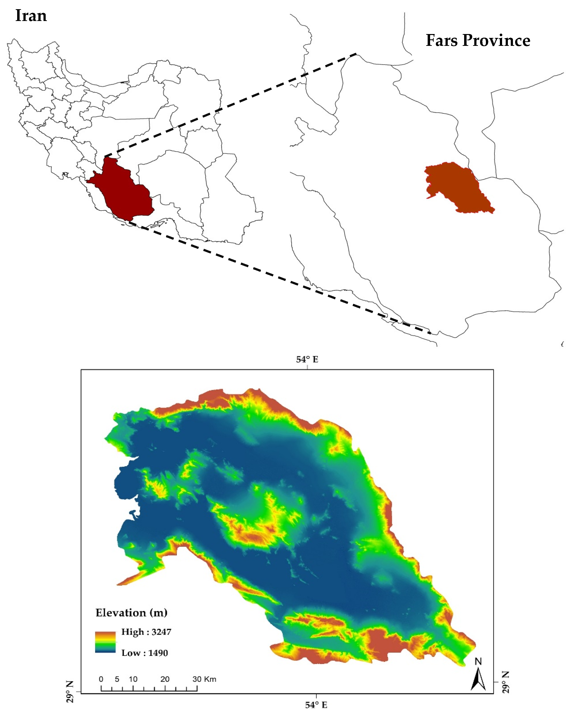
Figure 1. Location of the study area, Bakhtegan basin in Fars Province, southern Iran.
Land 12 00843 g001
Figure 2. Land subsidence (LS) occurrence. The first author took this photograph in the Bakhtegan basin on 18 June 2019.
Land 12 00843 g002
Figure 3. Subsidence predictor variables: (a) land use (LU), (b) land cover (LC), (c) lithology, (d) normalized difference salinity index (NDSI), (e) soil type, (f) climate type, (g) elevation, (h) slope, (i) aspect, (j) decline in groundwater level (DGWL), (k) depth of groundwater (DTGW), (l) curvature, (m) plain curvature, (n) profit curvature, (o) Topographic Wetness Index (TWI), (p) stream power index (SPI), (q) flow accumulation, (r) flow direction, (s) distance from faults (DFF), (t) distance from roads (DFR), (u) distance from an anticline (DFA), (v) distance from dams (DFD), (w) distance from mines (DFM), (x) distance from syncline (DFS), (y) distance from salt plain (DFSP), (z) distance from salt lake (DFSL), (zz) distance from residential areas (DFRA).
Land 12 00843 g003aLand 12 00843 g003b
Figure 4. Interferometric synthetic aperture radar (InSAR) processing conceptual flowchart (image developed by the authors).
Land 12 00843 g004
Figure 5. The study region’s land subsidence (LS) map (January to December 2019).
Land 12 00843 g005
Figure 6. Land subsidence (LS) susceptibility prediction maps via different machine learning models: random forests (RF; (a,b)), k-nearest neighbors (KNN; (c,d)), and classification and regression trees (CART; (e,f)).
Land 12 00843 g006aLand 12 00843 g006b
Figure 7. Results of the jackknife test in the various machine learning models: (a) random forests (RF), (b) k-nearest neighbors (KNN), and (c) classification and regression trees (CART). Abbreviations are described in Table 1.
Land 12 00843 g007
Table 1. Variables in land subsidence (LS) susceptibility modeling.
CriteriaVariables
HydrometeorologicalA decline in groundwater level (DGWL), depth of groundwater (DTGW), climate type, flow accumulation, flow direction
GeologicalLithology, soil type, normalized difference salinity index (NDSI)
GeomorphologicalElevation, slope, aspect, distance from anticline (DFA), distance from syncline (DFS), distance from salt plain (DFSP), distance from salt lake (DFSL), distance from fault (DFF), Topographic Wetness Index (TWI), stream power index (SPI), curvature, profile curvature, plan curvature
AnthropogenicLand use (LU), land cover (LC), distance from a dam (DFD), distance from road (DFR), distance from mine (DFM), distance from a residential area (DFRA)
Table 2. Area of land subsidence (LS) susceptibility classes in various machine learning (ML) models: random forests (RF), k-nearest neighbors (KNN), and classification and regression trees (CART).
Susceptibility ClassesRFKNNCART
AreaAreaArea
km2(%)km2(%)km2(%)
Very low35.6858.1334.0955.5434.0986.80
Low18.8430.7020.4533.3220.454.07
Moderate4.086.664.136.734.134.65
High0.821.340.661.080.661.32
Very high1.933.142.053.332.491.62
Table 3. Performance statistics of machine learning models (random forests (RF), k-nearest neighbors (KNN), and classification and regression trees (CART)) in land subsidence (LS) susceptibility prediction.
Performance StatisticsTrainingValidating
RFKNNCARTRFKNNCART
Standard deviation (STDEV)0.050.050.050.040.040.04
Root-mean-square error (RMSE)0.010.020.020.020.030.03
Nash–Sutcliffe efficiency (NSE)0.950.910.810.760.690.71
RMSE-observations standard deviation ratio (RSR)0.210.290.430.490.560.54
Correlation coefficient (COR)0.980.960.900.880.830.85
R-squared (R2)0.960.920.820.770.690.71
Kling–Gupta efficiency (KGE)0.890.810.880.780.740.75
Percent bias (PBIAS)0.601.801.800.709.508.60
Disclaimer/Publisher’s Note: The statements, opinions and data contained in all publications are solely those of the individual author(s) and contributor(s) and not of MDPI and/or the editor(s). MDPI and/or the editor(s) disclaim responsibility for any injury to people or property resulting from any ideas, methods, instructions or products referred to in the content.