Article

Mapping Ecological Infrastructure in a Cross-Border Regional Context

1
Institute for Environmental Sciences, University of Geneva, 66 Bd. Carl-Vogt, CH-1205 Geneva, Switzerland
2
Conservatory and Botanical Garden of the City of Geneva, Switzerland, 1 ch. de l’Impératrice, CH-1292 Chambésy, Switzerland
3
Geneva School of Engineering, Architecture and Landscape, HEPIA, University of Applied Sciences and Arts of Western Switzerland, 150 Route de Presinge, CH-1254 Jussy, Switzerland
*
Author to whom correspondence should be addressed.
Land 2023, 12(11), 2010; https://doi.org/10.3390/land12112010
Submission received: 5 July 2023 / Revised: 28 July 2023 / Accepted: 2 August 2023 / Published: 2 November 2023
(This article belongs to the Special Issue Sustainable Land-Use Dynamics and Green Infrastructure Mapping)

Abstract

:
Facing the decline of biodiversity worldwide, the conservation of the remaining natural and semi-natural areas is fundamental. To do so, the concept of green infrastructure has gained attention recently. This case study presents the method developed to identify the green infrastructure in a cross-border, urbanized territory between Switzerland and France in the area of influence of the city of Geneva. The first part of the methodology consists of calculating and mapping the inputs aggregated in four pillars: (i) the distribution of habitats as well as the predicted distribution of hundreds of plant and animal species, (ii) the supply of five ecosystem services, (iii) the functional connectivity for three animal species and the light pollution and (iv) five indices of landscape’s structure. These inputs are then used to run a prioritization model to identify the areas with the highest ecological interest according to these weighted inputs. The cross-border situation of this case study had impacts on the way the input data were gathered and weighted and on the way the output was created to consider the expectations of the three main local authorities involved, without creating any legal obligations on the implementation of the green infrastructure. As a positive sign of the usefulness of these results, the resulting maps were immediately transferred to the land use planners in charge of developing ambitious visions of the “Grand Genève” territory for 2050 in alignment with 10 objectives of ecological transition as recently agreed and signed by local authorities. The method presented in this article is flexible and includes a broad description of biodiversity, supporting a reliable network of areas with high ecological values for conservation purposes and human well-being.

1. Introduction

Global biodiversity is under a major crisis at every level and its genetic, species and ecosystem diversity is declining rapidly [1,2]. The destruction of natural habitats for agriculture and/or urbanization is the main cause of its decline and is directly linked to our way of occupying terrestrial and marine surfaces as well as to our consumption patterns [3,4,5,6,7]. Biological diversity decline might ultimately alter ecosystem functions such as productivity, stability and resilience, jeopardizing our food and water security as well as our socio-economic well-being [8,9,10,11,12,13,14,15,16,17]. Thus, the conservation of the remaining natural and semi-natural areas is fundamental, especially in urbanized environments where urbanization represents an additional pressure.
Green infrastructure (GI) is defined as a network of (semi-)natural areas allowing structural and functional connectivity of the landscape where biodiversity and ecosystem services are concentrated. The concept of GI fits perfectly the modern view of nature’s conservation that emphasizes the cohabitation of people and nature with sustainable and resilient interactions [18]. This new paradigm encompasses the common health of human societies and natural systems, highlighting our direct dependence upon ecosystems as described in the “One Health” concept [19,20]. GI is usually described as an interconnected network of (semi-)natural areas designed to deliver wide range of ecological, social and economic benefits [21,22,23], although several definitions have been used [24,25]. It is usually made up of large areas concentrating biological diversity and ecosystem service supply, linked with corridors allowing structural and functional connectivity [22,26]. GI is highly relevant in urban areas because it gives an ecological value to each element of the territory, focusing on the multifunctionality of the landscape. GI also integrates the nature-based solutions to mitigate the effects of global changes [26,27,28]. It is promoted at the European scale but also at the federal and cantonal scale in Switzerland [29,30,31]. In France, GI contributes directly to the policy on green and blue networks (http://www.trameverteetbleue.fr (accessed on 1 July 2023). Internationally, GI fits Target 3 of the urgent actions that need to be taken over the decade to 2030 from the 15th Conference of the Parties to the Convention on Biological Diversity, which proclaims to “Ensure and enable that by 2030 at least 30 per cent of terrestrial areas of particular importance for biodiversity and ecosystem functions and services, are effectively conserved and managed through ecologically representative, well-connected and equitably governed systems of protected areas and other effective area-based conservation measures, while ensuring that any sustainable use is fully consistent with conservation outcomes.” [32].
There is no consensus on the methodology nor the inputs that should be used in order to identify and map a GI [24]. This has led to confusions where the term “green infrastructure” was used in very divergent ways while several concepts and terms were referring to the same idea (e.g., ecological network, green corridors, green prints, etc.) [25]. For example, in highly urbanized environments, GI is often used as a greening method or as architectural elements such as green walls or green roofs [33]. In other situations, GI is restricted to areas supporting ecosystem supply only or protected lands [34,35,36,37,38,39]. More details of how GI is used in the scientific literature as well as the methods employed to identify it and the associated limits are available in Honeck et al. (2020) [26]. This literature review identified a methodological gap in the identification of GI where most of the articles do not consider all aspects of biodiversity conservation and GI’s definition.
The methodology employed here is based on the “three pillars” approach that has already been applied in Geneva, Switzerland [40]. This approach allows the consideration of all aspects of biodiversity conservation and respects the initial definition of GI [26]. The method is adapted here to aggregate the inputs in four pillars, the third and the fourth being initially grouped: (1) the diversity and distribution of species and habitats using species distribution models and a land use–land cover (LULC) map of the territory, (2) the supply of ecosystem services and (3) the functional and (4) the structural connectivity of the landscape. A spatial prioritization tool is used to select the network of areas with the highest ecological interest. The novelty of this article is the presentation of an application of the theoretical approach developed in Honeck et al. (2020) [26] on a cross-border territory, emphasizing the various methods used to calculate and integrate 2437 inputs for the identification of the GI. This exhaustive work can be used as a baseline for any territory aiming at mapping its own GI.
This article is focused on the prioritization of the GI network covering 30% of the territory of a regional cross-border agglomeration between France and Switzerland named “Greater Geneva”. This region is located in the European Alps and in the area of economic influence of the city of Geneva. In January 2023, the elected representatives of Greater Geneva signed the Charter for Greater Geneva in Transition with the desire to make the ecological transition the backbone of cross-border cooperation, recognizing that the erosion of life, the depletion of natural resources and climate degradation are our greatest threats [41]. The Charter sets out 10 strategic commitments to respect both the social floor and the ecological ceiling. The GI is fully in line with Objective 3 on Biodiversity of the Charter that aims at stopping the loss of natural habitats by 2050. It is also expected to have a positive impact on all other objectives.
This particular transboundary setting generated several issues that were addressed by the research questions presented below.
(i) What are the difficulties of gathering input data across borders?; (ii) What is the distribution of prioritization value across the studied areas?; (iii) What is the best 30 percent of the territory?; (iv) How can we accommodate the desire of each administrative entity to identify its own best 30%?; (v) What share of the identified GI is already protected? (vi) What are the difficulties in establishing GIs across borders?

2. Materials and Methods

2.1. Study Area

Greater Geneva is a cross-border territory between Switzerland and France of approximately 2000 km2 located around the city of Geneva. In its strict limits, it integrates three administrative entities grouped in two Swiss cantons (“Genève” and “Vaud” with the District of Nyon), and two French Departments (“Ain” and “Haute-Savoie”) with the “Pôle Métropolitain du Genevois Français”. This peculiar territory induces difficulties in compiling data because the taxonomy, the methods and the data availability vary from one administrative entity to another. However, the territory has a biogeographic consistency and is delimitated by mountain ranges, the Alps in the south-west and the Jura in the north-east, which justifies the GI assessment at this scale beyond borders. The region is particularly dynamic, and the population is growing rapidly due to the attractivity of the city of Geneva. The territory is dominated by urbanized areas and crops in the lowlands and forests and pastures in the mountainous areas.

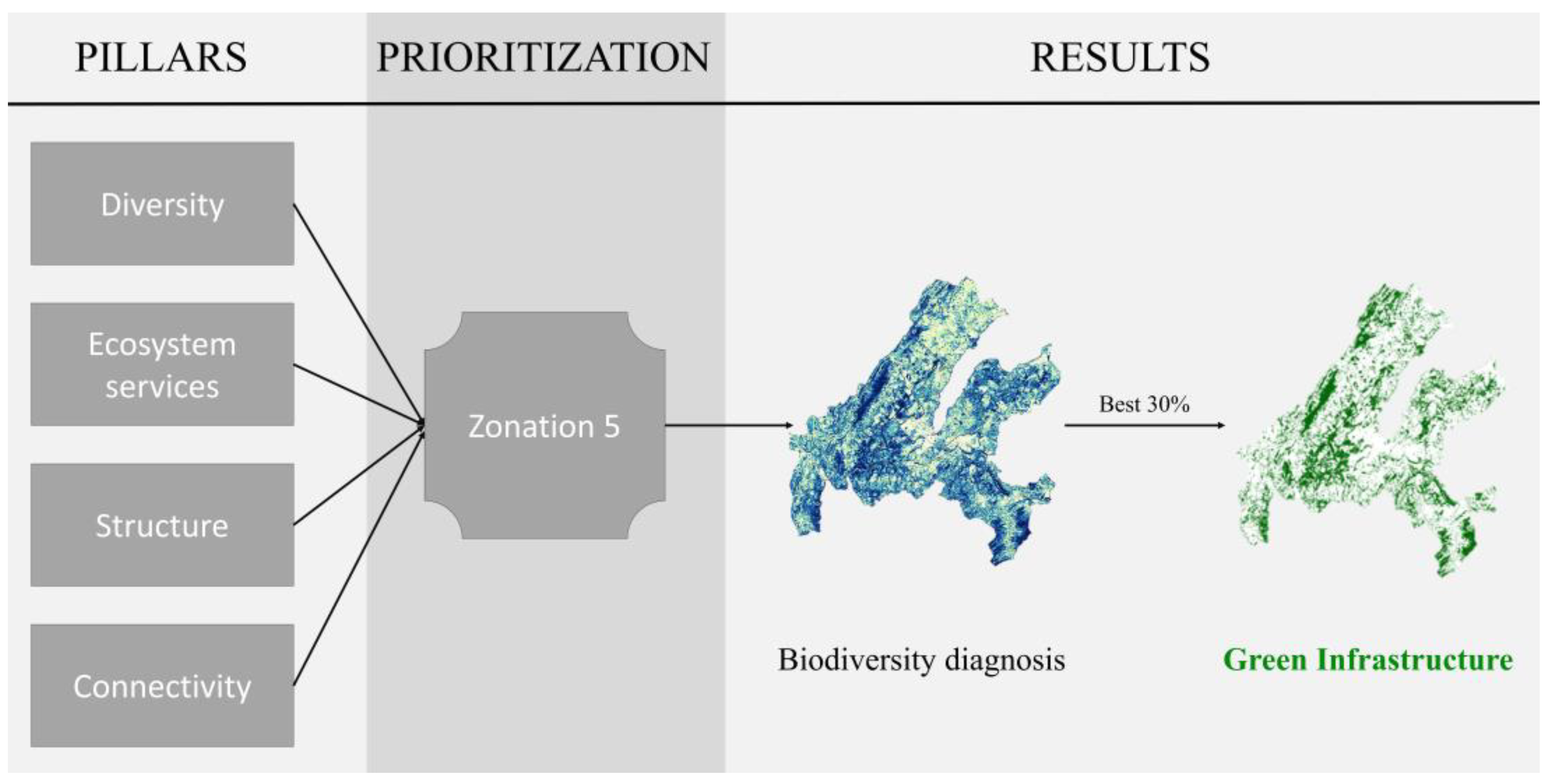
2.2. Method for Mapping the Ecological Infrastructure

According to the definition of GI, the inputs used to identify and map it have to consider several aspects of biodiversity and ecosystem service conservation [22,26,42]. For clarity, they were grouped into four main pillars: (1) the diversity pillar that includes the assessment of species and habitat distributions based on models and the aggregation of available LULC data; (2) the ecosystem service pillar that aims at mapping the supply of five regulating ecosystem services; (3) the connectivity pillar that includes maps of the functional connection for three animal species and light pollution; and (4) structural indices of the landscape based on the LULC categories. Once the inputs have been prepared at a spatial resolution of 25 m, they are included in a spatial prioritization tool set to classify every pixel of the territory according to its relative importance for biodiversity and ecosystems service conservation [42,43] (Figure 1). The method and the theoretical background used here were developed and explained exhaustively in two papers [26,40]. The inputs were selected according to the available data for describing the four pillars, their collinearity and their ecological meaning. The weight attributed to each of them was discussed in the working team and with the main stakeholders. The following sections explain the methods used to calculate and map the inputs.

2.3. Pillar 1: Species and Habitat Distribution

The assessment of the distributions of many species of plants and animals allows the identification of important areas for the conservation of specific richness. Furthermore, the inclusion of all distributions into the spatial prioritization process allows the selection of areas that are of the highest importance for rare species. The distribution of natural habitats also plays an important role in nature’s conservation by providing food and shelter to animals and plants but also by the maintenance of their ecological functions.

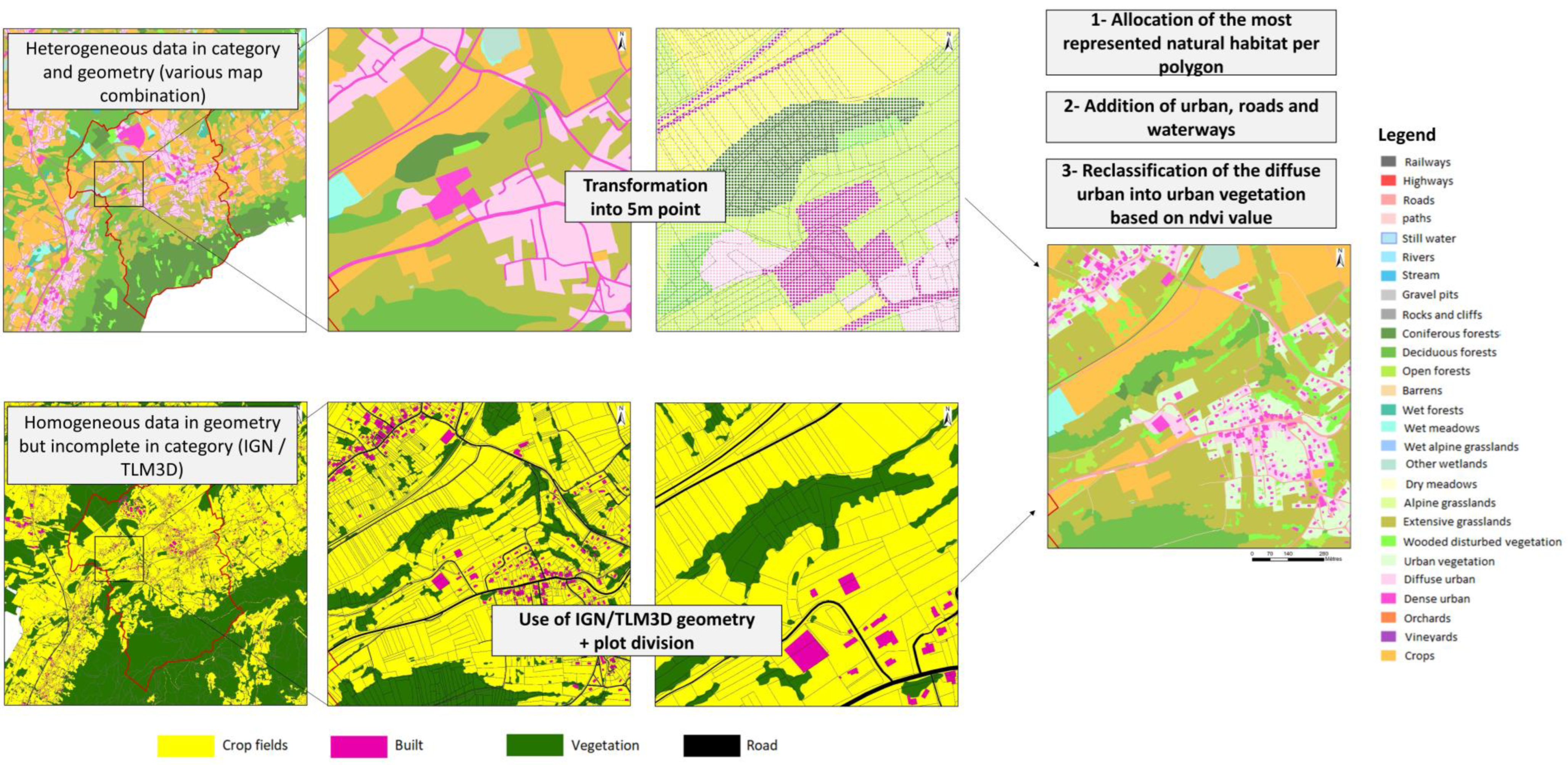
2.3.1. Natural Habitats

The distribution of habitats and more globally the LULC information are highly important for spatial planning at the regional scale but also for species distribution models (SDMs) [44].
The LULC map was created based on the compilation of the French and Swiss geomatic information sources, respectively named “Institut national de l’information géographique et forestière” (IGN, https://www.ign.fr/institut) and “Topographic Land Model” from SwissTopo (TLM3D, https://www.swisstopo.admin.ch/fr/geodata/landscape/tlm3d.html) (accessed on 1 July 2023). The data available across the study area were heterogenous in typology and geometry so both sources of information were used to homogenize the various maps into one. The geometry of the IGN map was extracted to divide the territory by administrative parcels that were transformed into polygons. Then, the habitat maps were transformed into five-meters points and added to the polygons where the most represented habitat was selected for each parcel. The dense urban environments, as well as the roads, railways, highways, rivers and running water, were then added. Finally, the diffuse urban environment class was created based on the presence of vegetation in the urban classes using NDVI information. More details of the method are presented in Figure 2.
The categories that were used in the prioritization process represent 19 (semi-)natural habitats, with the urban ones being excluded from this analysis. Each selected category was extracted as a unique input, ensuring the selection of at least a part of each (semi-) natural habitat in the final GI network by the prioritization process.

2.3.2. Species Distribution Modeling

SDM allows the creation of a covering map of habitat suitability based on the georeferenced observations of species’ individuals and predictive variables [45,46,47]. Several methods exist and have been used extensively in conservation [48,49,50,51]. Species’ occurrences were compiled from French and Swiss botanical conservatories and monitoring programs. Only observations between 2000 and 2020 and with a precision below 25 m were kept. To better conserve endangered species, we compiled the red list statuses from the different entities and selected the most threatened status. This ensures that the threats species are facing are not under-evaluated. At the end of the process, 585 species of animals and 1816 plants were selected. Predictive variables were selected based on their collinearity, ecological meaning and modeling performances in the study area and are presented in Table 1 [52]. The resolution of these variables is 25 m.
The chosen modeling algorithm was MaxEnt [53,54] (version 3.4.1) because it is widely used in SDM [55] and known to perform well especially with presence-only data [56,57]. The models were run using “Dismo” [58], “ENMeval” [59] and “sdm” [60] packages in R [61]. The default settings were kept except for the beta multiplier that was set to 2.00 to avoid over-fitting [62,63]. For each model, the occurrences were randomly split with 75% used for calibration and 25% for evaluating the model’s performances 10 times in a raw. Ten thousand background data were randomly created for each model. Then, for each species, a final model was calibrated with all occurrences available to map habitat suitability with all the information. More details about the modeling method and data selection process can be found in Sanguet et al. (2022) [52].
Table 1. Predictive variables used in the SDM.
VariablesDescriptionOrigin
TemperaturesMean annual temperatureWorldclim, R
PrecipitationsAnnual precipitationsWorldclim, R
ExpositionNorthness indexArcMap 10.2.1
SlopeContinuous slopeArcMap 10.2.1
Solar radiationsMean seasonal solar radiationArcMap 10.2.1
Landscape dominanceIndex of landscape dominationArcMap 10.2.1, modified from Weiss, 2001 [64]
CambisolCambisol proportion in the surrounding soilHengl et al., 2017 [65]
PodzolPodzol proportion in the surrounding soilHengl et al., 2017 [65]
Closed forestsDistribution of deciduous and coniferous forestsLULC map
Open forestsDistribution of opens forests and barrensLULC map
Urban areasDistribution of highly and moderately dense urban areasLULC map
TransportationDistribution of railways, paths, highways and roadsLULC map
Disturbed vegetationDistribution of urban and wooded disturbed vegetationLULC map
Natural meadowsDistribution of dry, alpine and extensive meadowsLULC map
AgricultureDistribution of crops, vineyards and orchardsLULC map
WetlandsDistribution of wet meadows, riverbeds and wet forestsLULC map

2.4. Pillar 2: Ecosystem Service Supply

The preservation of ecosystem services of regulation and support to biodiversity contributes to conserving the good functioning of ecosystems. Furthermore, the preservation of ecosystem services’ supply, as part of nature’s contributions to people and nature-based solutions, helps mitigate the detrimental effects of climate change or the consequences of extreme meteorological events. Other types of ecosystem services such as resource production or cultural services were not included in this work because they might induce the selection of areas with low quality or detrimental effects on biodiversity. Five ecosystem services were modeled and mapped using InVEST (version 3.12.0): the suitable areas for pollinators, the atmospheric carbon storage, the nutrient delivery ratio, the sediment delivery ratio and the leaf area index.

2.4.1. Suitable Areas for Pollinators

Pollinators are highly important for crop pollination and, as a consequence, for our food provision. Identifying their most suitable habitats to be integrated into the final GI network participates in maintaining the populations’ health and pollinators’ availability. The index calculated here represents a potential abundance of pollinators for each pixel of the resulting map based on their ecology, considering the quality and attractivity of the habitats for feeding and nesting habits. The “Crop Pollination” program was used in the software InVEST. Two tables are needed to run the model. The guild table contains the characteristics of 20 wild bee species while the biophysical table associates habitats with wild species’ traits and habits. Both tables were created based on a literature review and local expert knowledge to adjust the value to the local context (Table A1 and Table A2 in Appendix A). The optional farm map was not used. The model produces one map for each season (winter excluded) which were added to map the total suitability of the landscape.

2.4.2. Atmospheric Carbon Storage

Carbon dioxide (CO2) is a greenhouse gas massively rejected into the atmosphere by human activities and is the main cause of the observed global warming. The preservation of natural habitats known to store carbon avoids their destruction and thus the release of the stored carbon dioxide into the atmosphere. Preserving forest growth compensates for a part of our emissions and participates sequestrating carbon into organic matter and the soil. The mapping of this ecosystem service uses a biophysical table linking each habitat category to its carbon storage capacity. The table, named “Carbon pools” in the “Carbon Storage and Sequestration” program of InVEST, was adapted from the available data in InVEST’s documentation and is available in Appendix A (Table A3). Only the storage was measured and not the sequestration.

2.4.3. Nutrient Delivery Ratio

The “Nutrient Delivery Ratio” (NDR) program of InVEST calculates the flow of nutrients into the rivers and other water bodies or their retention in the soil’s upper layers. Excessive nutrient accumulation in water could impacts aquatic ecosystems composition and functioning. The NDR program models the landscape’s load and retention of nitrogen and phosphorous based on a biophysical table linking the LULC categories to their nutrient retention and load abilities, but also on the digital elevation model, a nutrient runoff proxy such as the annual precipitations, and the distribution of watersheds. The values of the biophysical table were adapted to the local context from the literature [66,67,68] as well as from the available data on the InVEST documentation [69] and is available in the Appendix A (Table A4). The Borselli K parameter was set to 2, the subsurface critical length to 200 m, the subsurface maximum retention efficiency to 0.8 and after several tests the threshold flow accumulation was set to 140. This last parameter adjusts the modelling of the location of temporary rivers based on the digital elevation model. The value was selected after several tests to better fit known permanent and temporary rivers on the territory. Several results were produced, and the effective retention map was kept. It represents the relative capacity of each pixel to retain nutrients.

2.4.4. Sediment Delivery Ratio

The “Sediment Delivery Ratio” program in InvEST models the flow of sediments and thus the erosion of the landscape. Erosion might induce a higher risk of landslides and a loss of organic matter in the soil. The preservation of areas reducing the risk of erosion is a nature-based solution and allows the mitigation and avoidance of natural hazards. The data and settings required for this model are relatively similar to the NDR model. The biophysical table was adapted from the existing data in the InVEST documentation [69] and the literature [70,71] and is available in Appendix A (Table A4). The values link each LULC category with its ability to reduce the loss in sediment and its management by humans to reduce the erosion. The erosivity and erodibility maps were downloaded from the European Soil Data Centre [72] and projected in the territory at 25 m resolution. The settings used were the following: threshold flow accumulation = 140, Borselli K parameter = 2, maximum SDTR value = 0.8, Borselli ICO parameter = 0.5, maximum L value = 122. The results are composed of several maps and the avoided sediment export was selected. It gives a value to each pixel according to their ability to avoid sediment export.

2.4.5. Leaf Area Index

Vegetation cover reduces the temperature and filters the air. Due to mitigating the effects of climate change and regulating the micro-climate, it is especially interesting to preserve green spaces in urban environments. This ability could be mapped by the leaf area index based on remote sensing images of the territory. The normalized differentiation vegetation index (NDVI) allows mapping of the greenness of a landscape and has been largely used to classify vegetation types [73,74]. The average maximum value of the NDVI in the territory was calculated based on the remote sensing images from Landsat-5, Landsat-7 and Landsat-8 and compiled in the Swiss Datacube [52,73,74,75]. Then, a formula was applicated to the raster to calculate the leaf area index (1) [76].
0.57 e ( 2.33 N D V I )

2.5. Pillar 3: Functional Connectivity

Functional connectivity ensures spatial connections between habitats and maintains species movements which are especially important for their resilience against climate change [77] and for gene-flow. According to their characteristics, shape, surface or fragmentation level, natural habitats’ quality and functions vary [78]. Functional connectivity corresponds to the relative ease of mobility in the landscape for a species and depends on the intrinsic characteristics of the species and the landscape [79,80]. Indeed, the same landscape could be used very differently from one animal to another. Thus, a well-connected territory should allow various kind of species movements such as daily movement, large-scale migration and dispersion, ultimately permitting gene flow across populations. Hence, the functional connectivity was studied by the identification of both the corridors and the areas constraining species’ movements for three animal species as well as by the mapping of light pollution, an essential factor for nocturnal species’ movements.

2.5.1. Combined Connectivity and Corridors

Three species with various spatial behaviors and using different habitat types were selected for these analyses: Cervus elaphus L. (red deer), Capreolus capreolus L. (roe deer) and Lepus europaeus P. (Brown hare). Two maps representing the global connectivity of the landscape as well as the constraining areas were modeled for each species. They are both based on two main inputs: the species reservoirs (or core areas) and a resistance matrix. Potential reservoirs of wild populations were calculated using species’ resistance and connectivity maps of the Greater Geneva region [81,82]. These maps were created using species’ habitat requirements and expert knowledge based on the LULC information of the territory. Ecological barriers to species’ movements such as buildings and fenced highways are taken into account, which means the resulting model excludes portions of the territory that are not used or accessible to the species.
The first map represents the energetic cost of crossing the habitats located on the animal’s path and thus the probability for it to move across the landscape. Cumulative costs were calculated using a workflow in GIS software between the species’ reservoirs, using a matrix allocating a resistance value to each LULC category of the territory. This method corresponds to the surface generalization of least-cost path models [82]. Hence, suitable habitats close to the reservoirs of the considered species’ population are easier to cross because of its low energetic cost, while unsuitable habitats are more energy intensive.
The second connectivity map emphasizes the areas constrained by the urban occupation. In other words, it represents how few or many alternative ways are available for wildlife to move from one point to another. CircuitScape (v0.1.0) software was used to compute this map based on the circuit theory [81,82,83]. The preservation of these constrained corridors ensures the connectivity of the landscape, even for the urbanized areas.

2.5.2. Light Pollution

The spatial organization of a landscape could be used differently depending on the animal. The spatial behaviors of nocturnal species do not only depend on the landscape’s structure but also on the artificial light of urban areas. Indeed, they need dark spaces to carry out their movements as well as other activities. Thus, the identification of light pollution allows the preservation of areas that are especially shaded and dark during the night and the identification of areas highly polluted by light. To do so, urban areas are transformed into light emitting spaces and the model is adjusted according to the altitude and the presence of forests or water bodies. The map was modeled by F. Tapissier in 2016 [84], before the current restrictions in the use of electricity and urban lighting. Many villages and urban areas now drastically reduce their nocturnal light, and the current map might over-represent current light pollution in the study area.

2.6. Pillar 4: Landscape Structure

Landscape structure, or structural connectivity, corresponds to the spatial arrangement of its LULC categories. The distribution and physical organization of the (semi-)natural habitats were assessed in the territory in order to identify areas with a high interest in conservation, based on five indices: the fragmentation (or the continuity) of natural areas, the soil permeability, the naturality of habitats, the diversity of (semi-)natural habitats and the identification of core natural areas.

2.6.1. Fragmentation

Natural habitats are considered fragmented when their distribution is discontinuous and patches are separated by ecological barriers, mostly anthropic land cover types and transportation networks [85]. The fragmented habitats have a reduced availability for species especially in an urban context. Indeed, sound, odors or light might prevent certain species from living at the margins of their natural habitat if it is surrounded by human-made infrastructures [86]. Furthermore, connected habitats favor species’ movements and migrations. One method to model and map habitat fragmentation is to calculate the MESH size that corresponds to the probability of two randomly picked pixels belonging to the same habitat patch [87]. To do so, the LULC map of the territory was transformed into two binary values, 1 for ecological anthropic barriers and 0 for (semi-)natural habitats. This raster was then used as input in the software Fragstat (v4.2) [88] and the “Effective mesh size (MESH)” program in the window “Aggregation” of the “Class metrics” category was selected. The moving window sampling strategy was used with a round radius of 200 m and a maximum of 50% border with no data. The resulting map was then modified to show the continuity of the natural habitats, which is the exact opposite of the fragmentation.

2.6.2. Soil Permeability

In an urban context, the environment is mostly impermeable, preventing water from being absorbed in the soil which increases the risk of flooding. This impermeability is mostly due to the use of concrete. Thus, saving permeable habitats is a nature-based solution to mitigate the effects of extreme weather events, maintain ecological functions linked to the water cycle and favor soil biodiversity. To map the permeability of the study area, the categories “highways”, “road” and “dense urban areas” were considered as impermeable while the other categories were permeable. This permeability layer favors the conservation of natural habitats in opposition to highly anthropic LULC categories.

2.6.3. Naturality

Naturality corresponds to the ecological quality of a habitat. A very anthropic LULC category would have a low naturality while a highly diverse, well-managed habitat with low disturbance would have a high naturality. This index allows ranking of the habitats according to their intrinsic quality in the study area. Using experts’ knowledge, all LULC categories were assigned a value between 1, corresponding to a very low naturality for urban areas, and 5, for the most interesting habitats. Then, a spatial focal statistic was applied to the raster using a 200 m radius to smooth the values and avoid class boundary effects. The map was exported at 25 m resolution.

2.6.4. Diversity of Natural Habitats

A high diversity of natural habitats favors a high species richness in a territory, especially when these habitats are equally distributed. Thus, the Shannon index [89] was used to calculate the diversity of natural habitats in the study area. To do so, the LULC categories were aggregated in seven classes based on their similarity, without considering dense urban areas and transportation. The classes are the following: meadows, lightly urban areas, natural cliffs and rocks, disturbed vegetation, forests, agriculture and wetlands. The model was run using Fragstat (v4.2), selecting “Shannon’s diversity index (SHDI)” in the “Diversity” window of the “Landscape metrics” class. The moving window sampling strategy was used with a round radius of 200 m and a maximum of 50% border/no data.

2.6.5. Core Areas

This input is complementary to the diversity of natural habitats because it identifies patches of habitat that are large enough to have a central core area free from the influence of neighboring habitats (edge effect). Indeed, some species need large areas of the same habitat to thrive. However, the influence of the neighboring habitats varies depending on their naturality and intrinsic characteristics. For example, an anthropic LULC category has a strong influence that could penetrate deeper into the natural habitat in the form of olfactive, chemical or light pollution. On the other hand, natural habitats have a lower influence between themselves, and their characteristics have a lower level of penetration. A core area would then correspond to an area free from any edge effect.
The modeling of the distribution of core areas necessitates two tables. The first one aggregates the habitats in categories based on their similarity. The second is a penetration matrix linking each category with each other with a distance of influence. The distance must be written using the raster’s metric system and be a multiple of its resolution. Here, the resolution of the raster is 25 m squared, so only multiples of 25 are accepted in the penetration matrix. The values used were based on experts’ knowledge and calibration tests. Then, core areas were mapped with Fragstat (v4.2) using “Core Area Median” in the “Core Area” window of the “Landscape Metrics” class. The moving window sampling strategy was used with a round radius of 200 m and a maximum of 50% border/no data.

2.7. Spatial Conservation Prioritization

Spatial conservation prioritization allows identification and mapping of the optimal compromise between the layers used as inputs, considering their allocated weight and other settings. We used the additive benefit function of Zonation 5 [43] to prioritize each pixel of the study area. The process starts by ranking all the pixels of the study area according to their ecological interest, then iteratively removes cells with the smallest marginal loss in terms of conservation value [43]. The additive benefit function prioritizes areas where many inputs have a high ecological value, thus selecting pixels with high richness over those with rare features. The resulting map is a raster in which pixels’ rank ranges between 0 for low conservation value and 1 for the relative highest ecological interest. Inputs should be used with the same logic in their pixels’ value, by which the most interesting areas that should be conserved should have a high value while low-quality areas have a low value.
The previously mentioned inputs were classified into four classes corresponding to the four pillars and attributed a weight depending on their quality and capacity to identify highly relevant areas for conservation. In total, 2437 inputs were used in the prioritization process, mostly species habitat suitability maps. The details of inputs and their associated weight are found in Table 2. The weights were established empirically by several trials that were discussed among the authors and with the stakeholder group.
The study area is composed of three administrative entities: the French territory named “Pôle Metropolitain”, the Canton of Geneva and the District of Nyon in the Canton of Vaud. We compared the output of an analysis covering the entire region, with an analysis combining the results of three subregions. According to the stakeholders, the final GI network should cover 30% of each of these three regions, even though their size and ecological quality differ. To do so, the prioritization was made over the whole territory but the identification of the best 30% has been made on the separate entities. As the Canton of Geneva has already had a GI identified in a previous work with the same methodology, it was integrated in the final results to preserve the coherence with the previous analysis.

3. Results

3.1. Identification of the Habitats

The LULC map presented in Figure 3 consists of a raster of 25 m resolution and 27 categories. It represents broad natural and semi-natural habitats as well as various land uses and urban environments. Having access to a homogenous, precise and well-covering LULC map is fundamental for the analysis carried in this work but also for having a common baseline between stakeholders and the various administrative entities, especially in a cross-border territory.

3.2. Maps Used as Inputs to the Final Prioritization

The inputs used in the prioritization process represent interesting results by themselves because some areas might not be selected in the final GI while representing a high interest for one of the inputs. The 2437 maps calculated and modeled were aggregated into 41 maps, available for consultation by local authorities and planners in the following link: https://sitv-qual.geneve.ch/portal/apps/webappviewer/index.html?id=f5865a0162d64efb8434644372c022c6 (accessed on 1 July 2023).
All the input variables and the outputs of the analysis are available on the Yareta system for scientific archives (Supplementary Material S1).

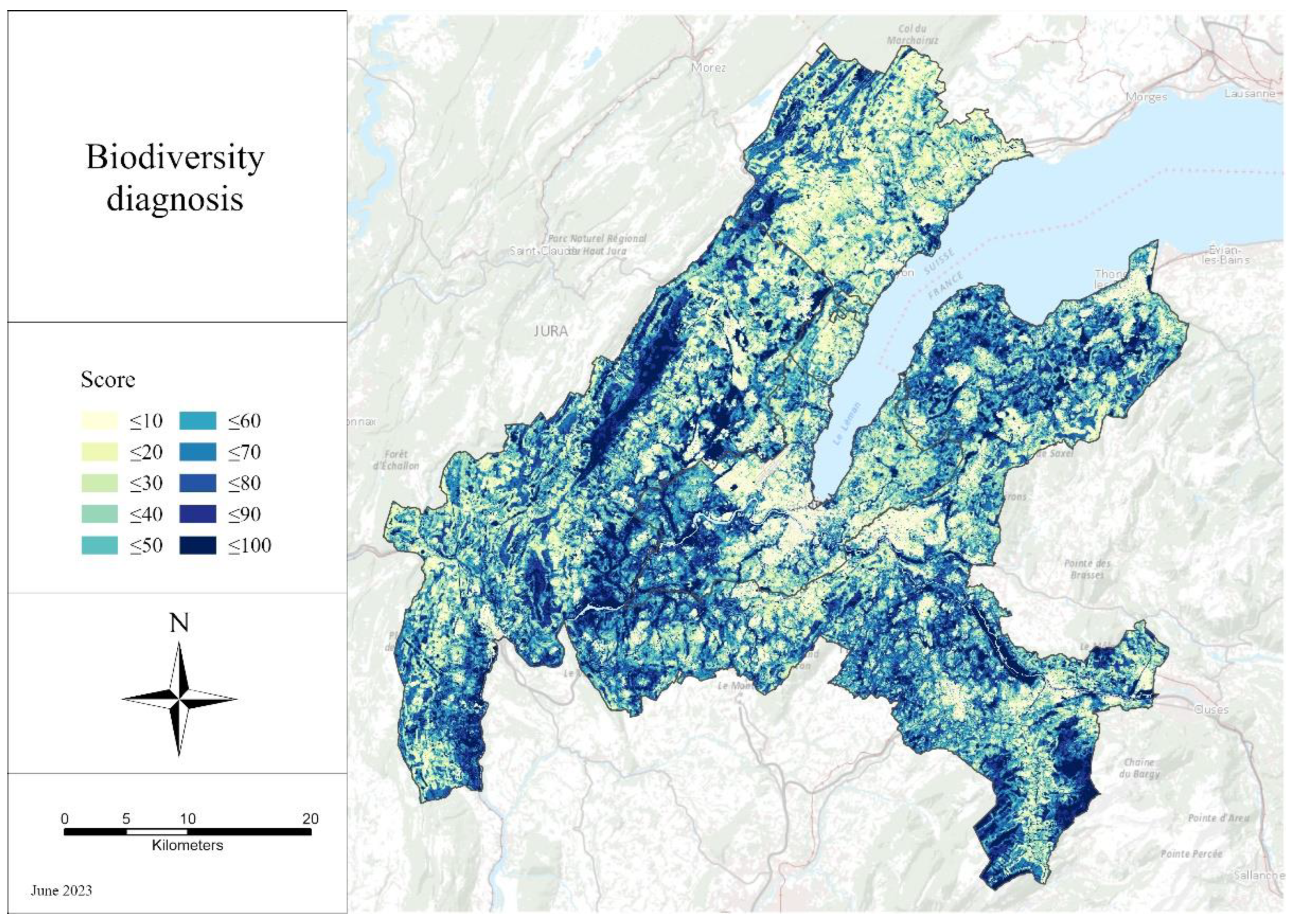
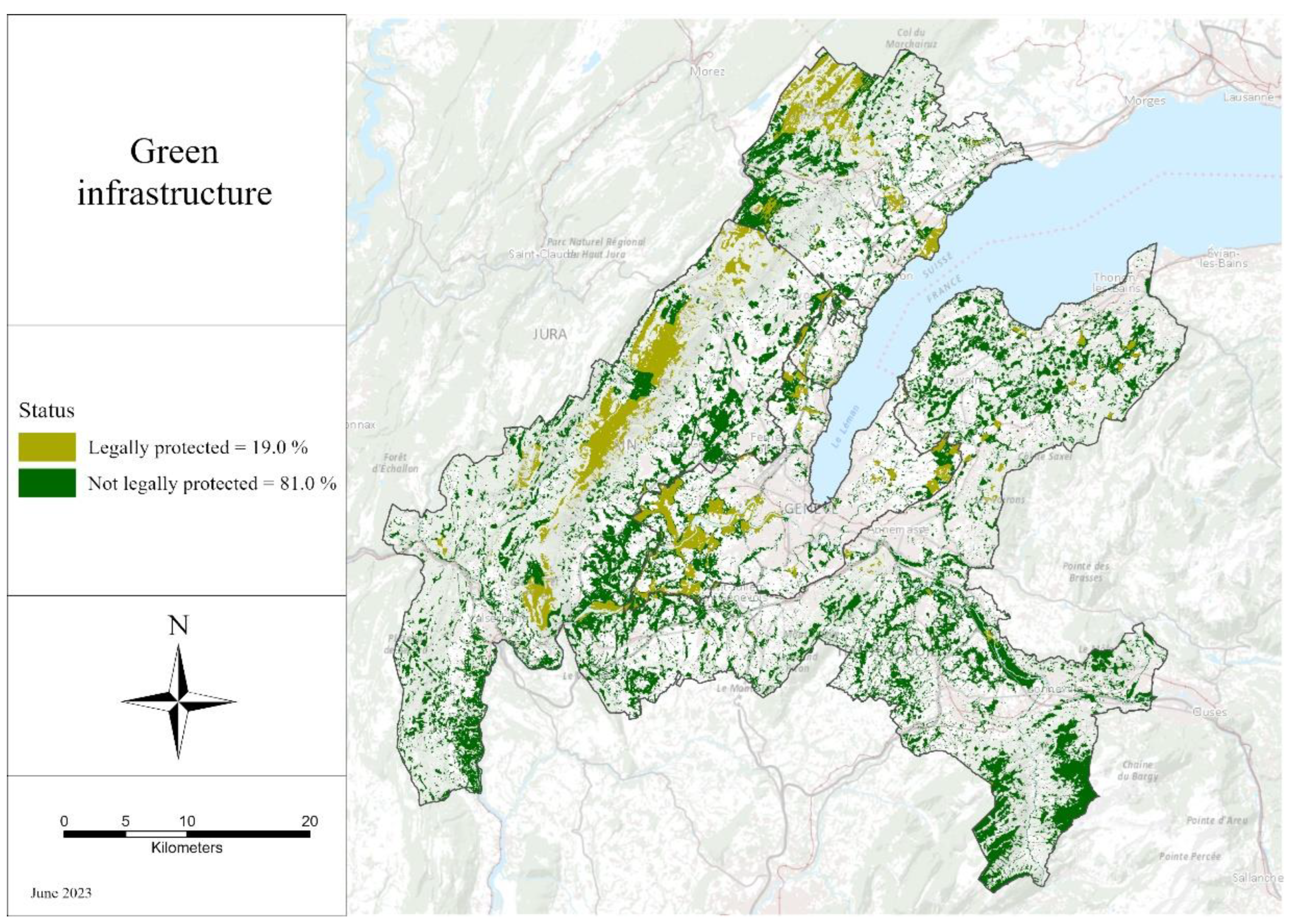
3.3. Biodiversity Diagnosis and GI

The main output of Zonation is the biodiversity diagnosis of the study area and is presented in Figure 4. This map represents the ranking of all pixels according to their ecological interest based on the inputs. The mountainous regions located on the north-eastern and the south-western parts of the territory seem of particular interest for conservation, which was expected because the anthropic pressure is lower in these areas compared to the lowlands, located at the center of the map. Urban centers are highly visible, especially the agglomeration of Geneva located in the middle of the study area where the conservation value of the cells is low. Forested areas in the lowlands also seem of high interest.
From this covering map, the top 30% pixels from the French administrative entity as well as the Swiss District of Nyon were independently extracted and then merge together with the GI of the Canton of Geneva identified in a previous work. This methodology, presented in Figure 5, allows identification of the GI for each administrative entity as well as for the whole territory to fit all political agendas.
The GI identified is visible in Figure 6. It is mostly made up of large patches well connected with many smaller isolated patches orbiting around the main core areas. Most of the GI is covered by closed forests (35%) and natural meadows (25%), while cultivated and diffuse urban areas both cover 16% of the GI, wetlands only 5% and open forests 3%. Closed forests thus represent more than one-third of the GI which is not surprising because they cover a similar portion of the whole study area, which means that they are not over-represented. However, natural meadows only cover 14% of the study area which means that they are over-represented in the GI, as are the wetlands only covering 1.5% of the study area. These habitats are thus highly important for biodiversity conservation in the region. On the other hand, cultivated areas are under-represented because they cover more than one-fifth of the study area. Another way of verifying which habitat is especially important for conservation is to look at the proportions of these habitats integrated into the GI. As previously mentioned, slightly more than one-quarter of all closed forests is integrated in the GI while this proportion rises to 53%, 97% and even 100% of all natural meadows, open forests and wetlands, respectively. This is a clear signal that these habitats are crucial elements of a functional, effective and reliable network of conservation.
Figure 6 also shows the proportion of the GI that is already protected. This result demonstrates that there is still a lot of effort to be made to preserve the areas with a high biodiversity value in the region for the benefit of future generations in the context of steady economic and population growth. As the best identified 30% of the territory will probably not obtain a legal status of protection, other efficient area-based measures (OECM) should be considered for their preservation as proposed by the IUCN [90].
The GI was initially identified by selecting the best 30% of the main Zonation output pixels over the whole study area, but the GI cover over the three territorial entities was disequilibrated because the main natural areas are found in the mountains located on the French side. This initial version would represent the best possible areas to conserve over the whole study area as there is no modification brought to the result of the prioritization process. However, with the methodology presented here, each entity has its own 30% GI cover in its territory. This is more equitable for the administrative entities and valuable for spatial conservation planning in order to reach the objective of dedicating 30% of each territory to nature’s conservation. The aggregated version of GI in the study area redistributed cells mainly from the patches in the mountainous areas to the more urban and cultivated areas in the lowlands as presented in Figure 7. Interestingly, most of the pixels that were removed from the initial version are either isolated or located at the margins of the main patches. Thus, the GI distribution from the aggregated version does not fundamentally change compared to the first version. This result means that the main patches identified in the initial “optimal” version are still included in the aggregated version. Thus, the conservation value of the aggregated GI network is still similar to the initial version, which is verified by the high spatial overlap of 88.1% between the two versions.

4. Discussion

4.1. Selection of Inputs

The inputs used in this methodology were selected based on their complementarity to avoid collinearity as much as possible, their representativity of the natural processes and their ease to be reproduced and explained to the authorities in charge of implementing the results. The final selection is the result of the separate assessment of each pillar in order to test the most reliable inputs for the local context and with the data available [26,40,52].
The distribution of natural habitats is key information for the modeling of the majority of inputs. Having access to a high-resolution LULC map with many detailed categories is fundamental for this work and its quality determines the accuracy of the resulting GI. Identifying many natural habitats allows consideration of each one of them in the prioritization process and thus ensures their representativity and conservation in the GI. However, for most of the inputs and species distribution models, eight categories are sufficient [52]. All species of plant and animal for which enough precise occurrences were available were modeled, with no distinction for their native status. However, a higher weight was given to species considered vulnerable, endangered or critically endangered in one of the red lists of the three territories. The inclusion of as many species as possible in the prioritization process creates a more reliable GI network by integrating all available distributions.
The selection of the ecosystem services was mainly based on their modeling availability in the software InVEST coupled with the perspective of conserving biodiversity. Many other ecosystems services were available but were linked with the production of resources and energy, or with the cultural value of the landscape, which might have deleterious outcomes for nature’s conservation. Although conserving highly biologically diverse areas usually has a positive influence on the preservation of qualitative and quantitative ecosystem service supplies, the opposite is not true [42,91]. The modeling of ecosystem services highly depends on values given to the settings and to the biophysical tables, as well as the quality of input maps. Specific values for the LULC categories used in the biophysical tables are mostly impossible to find in the literature, especially when they have to be adjusted to the local context. Furthermore, many settings require relative values, which depend on the characteristics of the inputs and of the territory. Thus, experts’ knowledge is highly valuable in this type of work. They should examine the inputs with care and verify the credibility of the resulting maps to iteratively calibrate the settings and tables.
The functional connectivity of the landscape for the species Cervus elaphus L. was calculated with the help of GPS trackers placed on several individuals [81,92]. The data collected allowed to define a resistance matrix based on the species’ habitat preferences, and thus represent a fundamental input for modeling the global connectivity and constrained zones. It has not been carried out for the two other species where inputs were based on experts’ knowledge [82]. It would be highly interesting to use GPS trackers for more individuals and species, but this method is expensive and not always applicable, especially for small animals. However, to better understand the functional connectivity of the territory, more animals could be studied such as amphibians, reptiles or small mammals, although large mammals’ results might serve as an umbrella for other species. Even though small animals’ movements do not reach the full extent of the study area, assessing their connectivity might also result in identifying corridors at a finer scale, resulting in a better representativeness of animal connectivity in the prioritization process. This assessment, however, is more challenging because of the lack of fine-scale data and its computational requirements.

4.2. Prioritization

The prioritization process was carried out over the whole territory but the best 30% was selected for each administrative entity. One limit of this approach could be the loss of connection at the edges of the three territorial entities, because the methodology does not consider that one patch should be entirely selected if its area is located on both sides of a border. This would be an important loss for the global structural and functional connectivity of the network as borders have no impact on species movements. However, this problem was not observed here, which could be explained by the fact that most of the borders are in the urbanized lowlands. In these areas, natural habitats with high ecological values are not so common and, thus, are easily identified by the methodology. This implies that the cross-border patches of natural habitats are selected on both sides of the border. Another reason that could explain this pattern is that the habitats located in the highlands and the lowlands are different. For example, deciduous forests are mainly found in the lowlands and coniferous forests in the highlands. Thus, the prioritization process would preferentially select patches of the same habitat, especially if it is not found anywhere else in the territory. It means that having access to a detailed map of the LULC information including many natural habitats might prevent the final network from being too much impacted by the spatial limits of the analysis.
The GI identified here covers the most interesting areas for nature’s conservation over the whole study area, considering the local context and administrative entities. However, it does not imply that areas located outside of the GI should not be considered for protection as well. This result is an overview of an optimal protection network to conserve all the aspects of the biodiversity and should be seen as a common aim for the territory. At a smaller scale, the conservation of natural habitats is fundamental because they could host important functions and diversity at this scale that are not represented or that are repetitive at the regional scale of the study area. Nevertheless, identifying and protecting a network of natural habitats is part of the solution to halt biodiversity loss but should be complemented, for example by lowering our impacts outside protected areas. Indeed, it is preferable to conserve, protect and restore more than not enough.

4.3. Perspectives

The proposed GI is still theoretical, and its effective implementation raises questions, especially regarding the legislation and the inclusion of private lands. There are already many protected areas with various appellations and legal basis in this cross-border area. Integrating conservation areas into the GI is an interesting idea, but the selection of which types of conservation area are integrated or not should be discussed among the stakeholders as some of them do not have strict legal basis. However, the integration of such large patches of protected areas might change the final distribution of the GI due to the prioritization process because most protected lands are made up of only a few natural habitats. Another solution would be to use the GI as informative data for spatial and urban planning to avoid the destruction of areas of high ecological interest, but the effective positive impact of GI on nature’s protection might be lower.
The ponderation used in the prioritization process was selected according to the value and interest attributed to the inputs by a group of experts. However, a more inclusive approach might be interesting, using, for example, the “best–worst method” based on the multiple criteria decision-making process [93]. This method allows sorting of the inputs from the best to the worst one and vice versa based on their conservation value. At the end of the process, a weight is automatically calculated and can be attributed to each input and each pillar. This approach is interesting but should be used with caution. Indeed, being able to classify the interest given to maps representing ecological processes is a complicated task and necessitates knowledge about the study area, its ecology and ecosystems, as well as about the method used to calculate the inputs which participates in evaluating their quality. Thus, the inclusion of the stakeholders is highly important, and they should be part of the process and decisions to model and map the inputs in order to fully understand their intrinsic meaning.

5. Conclusions

Most of the complex analyses presented in this work rely on the cross-border map of natural habitats that was first created for the Greater Geneva region. Without this common input the rest of the analyses would have been made difficult. All the environmental data (topography, water and climate, species, etc.) are by nature crossing borders. Most of the difficulties faced during this work are linked to the cross-border situation of the study area which means that a lot of work is still needed to share common data, classifications and methods at a larger scale to allow such analysis. However, this article proves that innovative insights, positive for the regional biodiversity, could emerge when the scientific community and the stakeholders from the different administrative entities work together. Indeed, the resulting maps from this article were immediately transferred to the land use planners in charge of developing ambitious visions of the “Greater Geneva” territory for 2050 in alignment with 10 objectives of ecological transition as recently agreed and signed by local authorities [41].
This article has shown that the territory of “Greater Geneva” could be classified from its best to its worse pixel, in terms of ecological value, using a prioritization process based on the use of many inputs grouped into four main pillars. This approach is very useful to identify the best areas that should be considered as hotspots of biodiversity and ecosystem services but also to identify coldspots that can be good candidates for potential urban developments or for ecological restoration. The results have shown that selecting the best 30% of each administrative entity of the study area was better accepted by stakeholders and did not fundamentally change the quality of the GI. The share of the identified GI that is already under protection is relatively low, demonstrating that much effort would be needed to reach the international target of 30% by 2030. However, the use of OECM as advocated by the IUCN could be a good solution to provide a status to the newly identified areas.
The GI identified in this work is the result of several years of research on the pillars and inputs on the same territory. The study area is well prospected and working together with naturalists, experts and the authorities in charge of the ecological conservation of the territory represents an asset to tune the settings to fit experts’ knowledge, field observations and political agendas. The methodology developed here is adaptable to other territories, depending on the data availability, and we believe it allows selection of the most interesting areas from an ecological perspective representing all aspects of biodiversity, ultimately resulting in a highly relevant and robust GI.

Supplementary Materials

S1: The inputs used in the prioritization process are available here: https://doi.org/10.26037/yareta:grduv33bcvcojfh5p64e2xwapi (accessed on 1 July 2023).

Author Contributions

Conceptualization, A.L., C.F. and N.W. (Nicolas Wyler); methodology, A.L., C.F. and N.W. (Nicolas Wyler); validation, all authors; formal analysis, A.S., B.G., L.U., L.H. and N.W. (Noé Waller); investigation, A.S., B.G., L.U., L.H. and N.W. (Noé Waller); data curation, A.S., B.G., L.U., L.H. and N.W. (Noé Waller); writing—original draft preparation, A.S.; writing—review and editing, A.L., N.W. (Nicolas Wyler), N.W. (Noé Waller), L.U., L.H., C.F., and B.G.; visualization, A.S. and N.W. (Noé Waller); supervision, A.L., C.F. and N.W. (Nicolas Wyler); project administration, A.L.; funding acquisition, A.L. and C.F. All authors have read and agreed to the published version of the manuscript.

Funding

This research was funded by the “Région de Nyon”, the “Pôle métropolitain français genevois”, the “Canton de Genève” and the Swiss Federal Office for the Environment.

Data Availability Statement

The inputs used in the prioritization process are available here: https://doi.org/10.26037/yareta:grduv33bcvcojfh5p64e2xwapi (accessed on 1 July 2023).

Acknowledgments

We wish to acknowledge the great collaboration with the representatives of the local authorities that gave us the mandate to do this research: Aurélie Stamm (Région de Nyon), Sylvie Vares (Pôle métropolitain français genevois) and Aline Blaser (Canton de Genève). We also thank Charlotte de Gouic for their collaboration on this project. This work is the continuation of scientific projects led by the group of experts GE21 from the University of Geneva (UNIGE), the Geneva School of Engineering, Architecture and Landscape (HEPIA), the Conservatory and Botanical Garden of Geneva (CJB) and the Cantonal Office for Agriculture and Nature (OCAN), more specifically Nathan Kuelling (UNIGE), Erica Honeck (UNIGE), Martin Schlaepfer (UNIGE), Alain Dubois (HEPIA), Pascal Martin (CJB), Bertrand Von Arx (OCAN) and Joëlle Kohler (OCAN). We would also like to thank the students that helped develop and test methods and data: Tess Calderon and Morgan Jan. Finally, we would like to thank the many institutions that shared their data which is a central theme especially in a cross-border territory: the Alpine and Franche-Comté National Botanical Conservatories (CBNA and CBNFC) together with all the contributors of the information system of the regional natural heritage inventory, Info Species, and its user community, as well as the Bird Protection League (LPO).

Conflicts of Interest

The authors declare no conflict of interest.

Appendix A. Biophysical Tables for Ecosystem Service Modeling

Table A1. Biophysical table used for the InVEST pollination model.
CodeCategoryNesting Cavity Availability IndexNesting Ground Availability IndexFloral Resources Spring IndexFloral Resources Summer IndexFloral Resources Autumn Index
1Highways00000
2Other wetlands000.30.50.2
3Path00000
4Railways0000.70.3
5Crops00100
6Still water00000
7Running water00000
8Coniferous forests00000
9Deciduous forests00000
10Wet forests100.70.30
11Open forests0.50.50.40.50.1
12Riverbeds010.30.60.1
13Gravel pits010.20.60.2
14Barrens010.10.80.1
15Rocks and cliffs01000
16Alpine grasslands010.10.80.1
17Extensive grasslands010.60.20.2
18Wet meadows100.30.50.2
19Dry meadows0.30.70.60.20.2
20Rivers00000
21Roads00000
22Stream00000
23Dense urban00000
24Diffuse urban0.50.50.60.30.1
25Wooded disturbed vegetation0.50.50.80.20
26Urban vegetation000.70.30
27Orchards010.90.10
28Vineyards010.90.10
Table A2. Guild table used for the InVEST pollination model.
SpeciesNesting Suitability Cavity IndexNesting Suitability Ground IndexForaging Activity Spring IndexForaging Activity Summer IndexForaging Activity Autumn IndexAlphaRelative Abundance
Andrena carantonica010.70.305121
Andrena chrysosceles010.60.402601
Andrena cineraria010.60.403001
Andrena dorsata010.40.606501
Andrena flavipes010.30.7011501
Andrena fulva011003151
Andrena haemorrhoa010.80.203731
Andrena minutula010.60.401121
Andrena nitida010.80.202881
Bombus hortorum0.50.50.30.60.16041
Bombus hypnorum100.30.60.12881
Bombus lapidarius0.50.50.20.60.215001
Bombus pascuorum0.50.50.30.40.323001
Bombus pratorum0.50.50.40.50.16741
Bombus terrestris0.50.50.30.50.215001
Lasioglossum calceatum010.40.40.210001
Lasioglossum malachurum010.30.50.36001
Lasioglossum morio010.20.40.4691
Lasioglossum politum010.20.60.2141
Osmia rufa100.60.406001
Table A3. Biophysical table used for the InVEST carbon storage model.
CodeCategoryC_aboveC_deadC_belowC_soil
1Highways0000
2Other wetlands6.50068.23
3Path0000
4Railways0000
5Crops3.510049.91
6Still water0000
7Running water0000
8Coniferous forests134.518.108.7055.4
9Deciduous forests134.518.108.7055.4
10Wet forests134.518.108.7055.4
11Open forests134.518.108.7055.4
12Riverbeds7.160026.31
13Gravel pits0000
14Barrens6.50068.23
15Rocks and cliffs0000
16Alpine grasslands4.980059.4
17Extensive grasslands4.980059.4
18Wet meadows6.40068.23
19Dry meadows4.980059.4
20Rivers0000
21Roads0000
22Stream0000
23Dense urban0000
24Diffuse urban0000
25Wooded disturbed vegetation20.4508.755.4
26Urban vegetation15.430053.4
27Orchards22.730064.76
28Vineyards5.360053.4
Table A4. Biophysical tables used for the InVEST sediment and nutrient delivery models (SDR and NDR).
CodeCategorySDRNDR
usle_cusle_pload_neff_ncrit_len_nproportion_subsurface_nload_peff_pcrit_len_pusle_c
1Highways00.516.60.12501.180.01250
2Other wetlands0116.70.515000.010.81500
3Path00.516.60.12501.180.01250
4Railways00.516.80.12501.180.01250
5Crops0.13840.99421550.651500.544.60.41500.1384
6Still water0111.40.052500.010.01250
7Running water0117.10.052500.010.01250
8Coniferous forests0.0012116.80.915002.360.61500.0012
9Deciduous forests0.0012116.80.915002.360.61500.0012
10Wet forests0.0012116.70.515000.010.81500.0012
11Open forests0.0012114.30.915002.360.61500.0012
12Riverbeds017.30.12501.180.01250
13Gravel pits017.30.12501.180.01250
14Barrens0.0219110.30.915002.360.61500.0219
15Rocks and cliffs017.30.12501.180.01250
16Alpine grasslands0.09030.994212.60.651500.510.50.51500.0903
17Extensive grasslands0.09030.9942740.651500.527.550.51500.0903
18Wet meadows0.0435116.70.515000.010.81500.0435
19Dry meadows0.043519.20.11500.52.360.61500.0435
20Rivers0117.10.052500.010.01250
21Roads00.516.60.12501.180.01250
22Stream0117.10.052500.010.01250
23Dense urban00.5170.125019.10.01250
24Diffuse urban00.516.40.425019.10.01250
25Wooded disturbed vegetation0.0219114.70.415002.360.61500.0219
26Urban vegetation0.026520.515.70.41500.42.360.61500.02652
27Orchards0.12320.9942740.651500.544.60.41500.1232
28Vineyards0.35270.9942740.651500.544.60.41500.3527

References

  1. IPBES. Media Release: Biodiversity and Nature’s Contributions Continue Dangerous Decline, Scientists Warn|IPBES-6 Plenary. 2018. Available online: https://www.ipbes.net/news/media-release-biodiversity-nature%E2%80%99s-contributions-continue-%C2%A0dangerous-decline-scientists-warn (accessed on 1 July 2023).
  2. IPBES. Global Assessment Report on Biodiversity and Ecosystem Services of the Intergovernmental Science-Policy Platform on Biodiversity and Ecosystem Services; Brondizio, E.S., Settele, J., Díaz, S., Ngo, H.T., Eds.; IPBES Secretariat: Bonn, Germany, 2019; 1148p. [Google Scholar] [CrossRef]
  3. Newbold, T.; Hudson, L.N.; Hill, S.L.L.; Contu, S.; Lysenko, I.; Senior, R.A.; Börger, L.; Bennett, D.J.; Choimes, A.; Collen, B.; et al. Global effects of land use on local terrestrial biodiversity. Nature 2015, 520, 45–50. [Google Scholar] [CrossRef] [PubMed]
  4. Pacifici, M.; Foden, W.B.; Visconti, P.; Watson, J.E.; Butchart, S.H.; Kovacs, K.M.; Scheffers, B.R.; Hole, D.G.; Martin, T.G.; Akçakaya, H.R.; et al. Assessing species vulnerability to climate change. Nat. Clim. Chang. 2015, 5, 215–224. [Google Scholar] [CrossRef]
  5. Sage, R.F. Global change biology: A primer. Glob. Chang. Biol. 2020, 26, 3–30. [Google Scholar] [CrossRef]
  6. Crenna, E.; Sinkko, T.; Sala, S. Biodiversity impacts due to food consumption in Europe. J. Clean. Prod. 2019, 227, 378–391. [Google Scholar] [CrossRef]
  7. Benton, T.G.; Bieg, C.; Harwatt, H.; Pudasaini, R.; Wellesley, L. Food System Impacts on Biodiversity Loss. In Three Levers for Food System Transformation in Support of Nature; Chatham House: London, UK, 2021; Available online: https://www.chathamhouse.org/2021/02/food-system-impacts-biodiversity-loss (accessed on 1 July 2023).
  8. Dawson, T.P.; Jackson, S.T.; House, J.I.; Prentice, I.C.; Mace, G.M. Beyond predictions: Biodiversity conservation in a changing climate. Science 2011, 332, 53–58. [Google Scholar] [CrossRef]
  9. McGill, B.J.; Dornelas, M.; Gotelli, N.J.; Magurran, A.E. Fifteen forms of biodiversity trend in the Anthropocene. Trends Ecol. Evol. 2015, 30, 104–111. [Google Scholar] [CrossRef]
  10. Scheffers, B.R.; Meester, L.D.; Bridge, T.C.L.; Hoffmann, A.A.; Pandolfi, J.M.; Corlett, R.T.; Butchart, S.H.M.; Pearce-Kelly, P.; Kovacs, K.M.; Dudgeon, D.; et al. The broad footprint of climate change from genes to biomes to people. Science 2016, 354, aaf7671. [Google Scholar] [CrossRef] [PubMed]
  11. Hector, A.; Schmid, B.; Beierkuhnlein, C.; Caldeira, M.C.; Diemer, M.; Dimitrakopoulos, P.G.; Finn, J.A.; Freitas, H.; Giller, P.S.; Good, J.; et al. Plant diversity and productivity experiments in European grasslands. Science 1999, 286, 1123–1127. [Google Scholar] [CrossRef]
  12. Naeem, S.; Thompson, L.J.; Lawler, S.P.; Lawton, J.H.; Woodfin, R.M. Declining biodiversity can alter the performance of ecosystems. Nature 1994, 368, 734–737. [Google Scholar] [CrossRef]
  13. Power, M.E.; Tilman, D.; Estes, J.A.; Menge, B.A.; Bond, W.J.; Mills, L.S.; Daily, G.; Castilla, J.C.; Lubchenco, J.; Paine, R.T. Challenges in the quest for keystones: Identifying keystone species is difficult—But essential to understanding how loss of species will affect ecosystems. BioScience 1996, 46, 609–620. [Google Scholar] [CrossRef]
  14. Tilman, D.; Downing, J.A. Biodiversity and stability in grasslands. Nature 1994, 367, 363–365. [Google Scholar] [CrossRef]
  15. Tilman, D.; Wedin, D.; Knops, J. Productivity and sustainability influenced by biodiversity in grassland ecosystems. Nature 1996, 379, 718–720. [Google Scholar] [CrossRef]
  16. Walker, B.H. Biodiversity and ecological redundancy. Conserv. Biol. 1992, 6, 18–23. [Google Scholar] [CrossRef]
  17. Cardinale, B.J.; Duffy, J.E.; Gonzalez, A.; Hooper, D.U.; Perrings, C.; Venail, P.; Narwani, A.; Mace, G.M.; Tilman, D.; Wardle, D.A. Biodiversity loss and its impact on humanity. Nature 2012, 486, 59–67. [Google Scholar] [CrossRef]
  18. Mace, G.M. Whose conservation? Science 2014, 345, 1558–1560. [Google Scholar] [CrossRef]
  19. One Health Initiative Task Force. One Health: A New Professional Imperative; American Veterinary Medical Association: Schaumburg, IL, USA, 2008. [Google Scholar]
  20. Mace, G. Ecosystem services: Where is the discipline heading? In Routledge Handbook of Ecosystem Services; Routledge: London, UK, 2016; pp. 602–606. [Google Scholar]
  21. Benedict, M.A.; McMahon, E.T. Green Infrastructure: Linking Landscapes and Communities; Island Press: Washington, DC, USA, 2006. [Google Scholar]
  22. da Silva, J.M.C.; Wheeler, E. Ecosystems as infrastructure. Perspect. Ecol. Conserv. 2017, 15, 32–35. [Google Scholar] [CrossRef]
  23. European Environment Agency. Spatial Analysis of Green Infrastructure in Europe; Technical report No 2/2014; EEA: Brussels, Belgium, 2014.
  24. Wang, J.; Banzhaf, E. Towards a better understanding of green infrastructure: A critical review. Ecol. Indic. 2018, 85, 758–772. [Google Scholar] [CrossRef]
  25. Firehock, K. Strategic Green Infrastructure Planning—A Multi-Scale Approach; Island Press: Washington, DC, USA, 2015. [Google Scholar]
  26. Honeck, E.; Sanguet, A.; Schlaepfer, M.A.; Wyler, N.; Lehmann, A. Methods for identifying green infrastructure. SN Appl. Sci. 2020, 2, 1916. [Google Scholar] [CrossRef]
  27. Naumann, S.; Davis, M.; Kaphengst, T.; Pieterse, M.; Rayment, M. Design, Implementation and Cost Elements of Green Infrastructure Projects; Final report; European Commission: Brussels, Belgium, 2011; p. 138. [Google Scholar]
  28. Cohen-Shacham, E.; Walters, G.; Janzen, C.; Maginnis, S. Nature-Based Solutions to Address Global Societal Challenges; IUCN: Gland, Switzerland, 2016; Volume 97, pp. 2016–2036. [Google Scholar] [CrossRef]
  29. DETA; DGAN; CCDB. Stratégie Biodiversité Genève 2030 (SBG-2030); République et canton de Genève: Geneva, Switzerland, 2018. [Google Scholar]
  30. OFEV. Plan d’action du Conseil Fédéral 2017: Plan D’action Stratégie Biodiversité Suisse; Office Fédéral de l’environnement OFEV: Berne, Switzerland, 2017; p. 53. [Google Scholar]
  31. OFEV. Infrastructure Ecologique. Guide de Travail Pour la Planification Cantonale Dans le Cadre de la Période de Convention-Programme 2020–2024; Office Fédéral de l’environnement OFEV: Berne, Switzerland, 2021; Version 1.0. [Google Scholar]
  32. CBD/COP/15/L.25 18 December 2022, Montreal, Canada. Available online: https://www.cbd.int/doc/c/e6d3/cd1d/daf663719a03902a9b116c34/cop-15-l-25-en.pdf (accessed on 1 July 2023).
  33. Irga, P.J.; Braun, J.T.; Douglas, A.N.J.; Pettit, T.; Fujiwara, S.; Burchett, M.D.; Torpy, F.R. The distribution of green walls and green roofs throughout Australia: Do policy instruments influence the frequency of projects? Urban For. Urban Green. 2017, 24, 164–174. [Google Scholar] [CrossRef]
  34. Elbakidze, M.; Angelstam, P.; Yamelynets, T.; Dawson, L.; Gebrehiwot, M.; Stryamets, N.; Manton, M. A bottom-up approach to map land covers as potential green infrastructure hubs for human well-being in rural settings: A case study from Sweden. Landsc. Urban Plan. 2017, 168, 72–83. [Google Scholar] [CrossRef]
  35. Lynch, A.J. Is it good to be green? Assessing the ecological results of county green infrastructure planning. J. Plan. Educ. Res. 2016, 36, 90–104. [Google Scholar] [CrossRef]
  36. Park, H.; Kramer, M.; Rhemtulla, J.M.; Konijnendijk, C.C. Urban food systems that involve trees in Northern America and Europe: A scoping review. Urban For. Urban Green. 2019, 45, 126360. [Google Scholar] [CrossRef]
  37. Donaldson, G.H.; João, E.M. Using green infrastructure to add value and assist place-making in public realm developments. Impact Assess. Proj. Apprais. 2020, 38, 464–478. [Google Scholar] [CrossRef]
  38. Fattorini, S.; Galassi, D.M. Role of urban green spaces for saproxylic beetle conservation: A case study of tenebrionids in Rome, Italy. J. Insect Conserv. 2016, 20, 737–745. [Google Scholar] [CrossRef]
  39. Shwartz, A.; Turbé, A.; Julliard, R.; Simon, L.; Prévot, A.C. Outstanding challenges for urban conservation research and action. Glob. Environ. Chang. 2014, 28, 39–49. [Google Scholar] [CrossRef]
  40. Honeck, E.; Moilanen, A.; Guinaudeau, B.; Wyler, N.; Schlaepfer, M.A.; Martin, P.; Sanguet, A.; Urbina, L.; von Arx, B.; Massy, J.; et al. Implementing Green Infrastructure for the Spatial Planning of Peri-Urban Areas in Geneva, Switzerland. Sustainability 2020, 12, 1387. [Google Scholar] [CrossRef]
  41. Chartre Grand Genève en Transition, Grand Genève. 2023. Available online: https://www.grand-geneve.org/wp-content/uploads/Charte_Grand_Geneve_en_Transition_2023.pdf (accessed on 1 July 2023).
  42. Snäll, T.; Lehtomaki, J.; Arponen, A.; Elith, J.; Moilanen, A. Green infrastructure design based on spatial conservation prioritization and modeling of biodiversity features and ecosystem services. Environ. Manag. 2016, 57, 251–256. [Google Scholar] [CrossRef]
  43. Moilanen, A.; Wilson, K.A.; Possingham, H. Spatial Conservation Prioritization: Quantitative Methods and Computational Tools; Oxford University Press: Oxford, UK, 2009. [Google Scholar]
  44. Austin, M.P.; Van Niel, K.P. Improving species distribution models for climate change studies: Variable selection and scale. J. Biogeogr. 2011, 38, 1–8. [Google Scholar] [CrossRef]
  45. Guisan, A.; Zimmermann, N.E. Predictive habitat distribution models in ecology. Ecol. Model. 2000, 135, 147–186. [Google Scholar] [CrossRef]
  46. Soberón, J.; Nakamura, M. Niches and distributional areas: Concepts, methods, and assumptions. Proc. Natl. Acad. Sci. USA 2009, 106 (Suppl. 2), 19644–19650. [Google Scholar] [CrossRef]
  47. Hirzel, A.H.; Le Lay, G. Habitat suitability modelling and niche theory. J. Appl. Ecol. 2008, 45, 1372–1381. [Google Scholar] [CrossRef]
  48. Lehmann, A.; Overton, J.M.; Austin, M.P. Regression models for spatial prediction: Their role for biodiversity and conservation. Biodivers. Conserv. 2002, 11, 2085–2092. [Google Scholar] [CrossRef]
  49. Lehmann, A.; Overton, J.M.; Leathwick, J.R. GRASP: Generalized regression analysis and spatial prediction. Ecol. Model. 2002, 157, 189–207. [Google Scholar] [CrossRef]
  50. Guisan, A.; Tingley, R.; Baumgartner, J.B.; Naujokaitis-Lewis, I.; Sutcliffe, P.R.; Tulloch, A.I.; Regan, T.J.; Brotons, L.; McDonald-Madden, E.; Mantyka-Pringle, C.; et al. Predicting species distributions for conservation decisions. Ecol. Lett. 2013, 16, 1424–1435. [Google Scholar] [CrossRef] [PubMed]
  51. Guisan, A.; Thuiller, W.; Zimmermann, N.E. Habitat Suitability and Distribution Models: With Applications in R; Cambridge University Press: Cambridge, UK, 2017. [Google Scholar]
  52. Sanguet, A.; Wyler, N.; Petitpierre, B.; Honeck, E.; Poussin, C.; Martin, P.; Lehmann, A. Beyond topo-climatic predictors: Does habitats distribution and remote sensing information improve predictions of species distribution models? Glob. Ecol. Conserv. 2022, 39, e02286. [Google Scholar] [CrossRef]
  53. Phillips, S.J.; Dudík, M.; Schapire, R.E. A maximum entropy approach to species distribution modeling. In Proceedings of the Twenty-First International Conference on Machine Learning, Banff, AB, Canada, 4–8 July 2004; p. 83. [Google Scholar] [CrossRef]
  54. Phillips, S.J.; Anderson, R.P.; Schapire, R.E. Maximum entropy modeling of species geographic distributions. Ecol. Model. 2006, 190, 231–259. [Google Scholar] [CrossRef]
  55. Guillera-Arroita, G.; Lahoz-Monfort, J.J.; Elith, J.; Gordon, A.; Kujala, H.; Lentini, P.E.; McCarthy, M.A.; Tingley, R.; Wintle, B.A. Is my species distribution model fit for purpose? Matching data and models to applications. Glob. Ecol. Biogeogr. 2015, 24, 276–292. [Google Scholar] [CrossRef]
  56. Elith, J.; Graham, C.H.; Anderson, R.P.; Dudík, M.; Ferrier, S.; Guisan, A.; Hijmans, R.J.; Huettmann, F.; Leathwick, J.R.; Lehmann, A. Novel methods improve prediction of species’ distributions from occurrence data. Ecography 2006, 29, 129–151. [Google Scholar] [CrossRef]
  57. Hijmans, R.J.; Graham, C.H. The ability of climate envelope models to predict the effect of climate change on species distributions. Glob. Chang. Biol. 2006, 12, 2272–2281. [Google Scholar] [CrossRef]
  58. Hijmans, R.J.; Phillips, S.; Leathwick, J.; Elith, J.; Hijmans, M.R.J. Package ‘dismo’. Circles 2023, 9, 1–68. [Google Scholar]
  59. Muscarella, R.; Galante, P.J.; Soley-Guardia, M.; Boria, R.A.; Kass, J.M.; Uriarte, M.; Anderson, R.P. ENM eval: An R package for conducting spatially independent evaluations and estimating optimal model complexity for Maxent ecological niche models. Methods Ecol. Evol. 2014, 5, 1198–1205. [Google Scholar] [CrossRef]
  60. Naimi, B.; Araújo, M.B. SDM: A reproducible and extensible R platform for species distribution modelling. Ecography 2016, 39, 368–375. [Google Scholar] [CrossRef]
  61. R Core Team. R: A Language and Environment for Statistical Computing; R Foundation for Statistical Computing: Vienna, Austria, 2019; Available online: https://www.R-project.org/ (accessed on 1 July 2023).
  62. Costa, G.C.; Nogueira, C.; Machado, R.B.; Colli, G.R. Sampling bias and the use of ecological niche modeling in conservation planning: A field evaluation in a biodiversity hotspot. Biodivers. Conserv. 2010, 19, 883–899. [Google Scholar] [CrossRef]
  63. Radosavljevic, A.; Anderson, R.P. Making better Maxent models of species distributions: Complexity, overfitting and evaluation. J. Biogeogr. 2014, 41, 629–643. [Google Scholar] [CrossRef]
  64. Weiss, A. Topographic position and landforms analysis. In Proceedings of the Poster Presentation, ESRI User Conference, San Diego, CA, USA, 9–13 July 2001; Volume 200. Available online: http://www.jennessent.com/downloads/TPI-poster-TNC_18x22.pdf (accessed on 1 July 2023).
  65. Hengl, T.; Mendes de Jesus, J.; Heuvelink, G.B.; Ruiperez Gonzalez, M.; Kilibarda, M.; Blagotić, A.; Shangguan, W.; Wright, M.N.; Geng, X.; Bauer-Marschallinger, B.; et al. SoilGrids250m: Global gridded soil information based on machine learning. PLoS ONE 2017, 12, e0169748. [Google Scholar] [CrossRef]
  66. Zobrist, J.; Reichert, P. Bayesian estimation of export coefficients from diffuse and point sources in Swiss watersheds. J. Hydrol. 2006, 329, 207–223. [Google Scholar] [CrossRef]
  67. Bai, Y.; Ochuodho, T.O.; Yang, J. Impact of land use and climate change on water-related ecosystem services in Kentucky, USA. Ecol. Indic. 2019, 102, 51–64. [Google Scholar] [CrossRef]
  68. Redhead, J.W.; May, L.; Oliver, T.H.; Hamel, P.; Sharp, R.; Bullock, J.M. National scale evaluation of the InVEST nutrient retention model in the United Kingdom. Sci. Total Environ. 2018, 610, 666–677. [Google Scholar] [CrossRef]
  69. Natural Capital Project. 2017. Available online: https://naturalcapitalproject.stanford.edu/ (accessed on 1 July 2023).
  70. Renard, K.G. Predicting Soil Erosion by Water: A Guide to Conservation Planning with the Revised Universal Soil Loss Equation (RUSLE); United States Government Printing: Washington, DC, USA, 1997.
  71. Jaligot, R.; Chenal, J.; Bosch, M. Assessing spatial temporal patterns of ecosystem services in Switzerland. Landsc. Ecol. 2019, 34, 1379–1394. [Google Scholar] [CrossRef]
  72. European Soil Data Centre. Available online: https://esdac.jrc.ec.europa.eu/ (accessed on 2 December 2022).
  73. Gamon, J.A.; Field, C.B.; Goulden, M.L.; Griffin, K.L.; Hartley, A.E.; Joel, G.; Penuelas, J.; Valentini, R. Relationships between NDVI, canopy structure, and photosynthesis in three Californian vegetation types. Ecol. Appl. 1995, 5, 28–41. [Google Scholar] [CrossRef]
  74. Geerken, R.; Zaitchik, B.; Evans, J.P. Classifying rangeland vegetation type and coverage from NDVI time series using Fourier Filtered Cycle Similarity. Int. J. Remote Sens. 2005, 26, 5535–5554. [Google Scholar] [CrossRef]
  75. Swiss Datacube. Available online: https://www.swissdatacube.org/ (accessed on 1 June 2021).
  76. Saito, K.; Ogawa, S.; Aihara, M.; Otowa, K. Estimation of LAI and Forest Management on Okutama. In Proceedings of the 22nd Asian Conference on Remote Sensing, Singapore, 5–7 November 2001; pp. 11–17. [Google Scholar]
  77. Pauls, S.U.; Nowak, C.; Bálint, M.; Pfenninger, M. The impact of global climate change on genetic diversity within populations and species. Mol. Ecol. 2013, 22, 925–946. [Google Scholar] [CrossRef]
  78. Tischendorf, L.; Fahrig, L. On the usage and measurement of landscape connectivity. Oikos 2000, 90, 7–19. [Google Scholar] [CrossRef]
  79. Taylor, P.D.; Fahrig, L.; Henein, K.; Merriam, G. Connectivity is a vital element of landscape structure. Oikos 1993, 68, 571–573. [Google Scholar] [CrossRef]
  80. With, K.A.; Gardner, R.H.; Turner, M.G. Landscape connectivity and population distributions in heterogeneous environments. Oikos 1997, 78, 151–169. [Google Scholar] [CrossRef]
  81. Urbina, L.; Fischer, C.; Ray, N.; Lehmann, A. Modelling red deer functional connectivity at regional scale in a human dominated landscape. Front. Environ. Sci. 2023, 11, 1198168. [Google Scholar] [CrossRef]
  82. Urbina, L.; Lehmann, A.; Huber, L.; Fischer, C. Combining multi-species connectivity modelling with expert knowledge to inform the green infrastructure design. 2023; under review. [Google Scholar]
  83. Anantharaman, R.; Hall, K.; Shah, V.B.; Edelman, A. Circuitscape in Julia: High Performance Connectivity Modelling to Support Conservation Decisions. JuliaCon Proc. 2020, 1, 58. [Google Scholar] [CrossRef]
  84. © Frederic Tapissier/AVEX/Cartes de Pollution Lumineuse. 2016. Available online: https://www.avex-asso.org/dossiers/wordpress/la-pollution-lumineuse-light-pollution/cartes-de-pollution-europeenne-avex-2016 (accessed on 1 July 2023).
  85. Lord, J.M.; Norton, D.A. Scale and the spatial concept of fragmentation. Conserv. Biol. 1990, 4, 197–202. [Google Scholar] [CrossRef]
  86. Fahrig, L. Effects of habitat fragmentation on biodiversity. Annu. Rev. Ecol. Evol. Syst. 2003, 34, 487–515. [Google Scholar] [CrossRef]
  87. Jaeger, J.A. Landscape division, splitting index, and effective mesh size: New measures of landscape fragmentation. Landsc. Ecol. 2000, 15, 115–130. [Google Scholar] [CrossRef]
  88. McGarigal, K.; Cushman, S.A.; Ene, E. FRAGSTATS v4: Spatial Pattern Analysis Program for Categorical Maps. 2023. Available online: https://www.fragstats.org (accessed on 1 July 2023).
  89. Pielou, E.C. Shannon’s formula as a measure of specific diversity: Its use and misuse. Am. Nat. 1966, 100, 463–465. [Google Scholar] [CrossRef]
  90. IUCN WCPA Task Force on OECMs. Recognising and Reporting Other Effective Area-Based Conservation Measures; IUCN, International Union for Conservation of Nature: Gland, Switzerland, 2019. [Google Scholar] [CrossRef]
  91. Manhães, A.P.; Mazzochini, G.G.; Oliveira-Filho, A.T.; Ganade, G.; Carvalho, A.R. Spatial associations of ecosystem services and biodiversity as a baseline for systematic conservation planning. Divers. Distrib. 2016, 22, 932–943. [Google Scholar] [CrossRef]
  92. Fischer, C.; Ranzoni, J. Assessment of the functionality of wildlife corridors used by red deer in the Geneva basin. Schweizerische Zeitschrift für Forstwesen 2017, 168, 299–304. [Google Scholar] [CrossRef]
  93. Rezaei, J. A Concentration Ratio for Non-Linear Best Worst Method. Int. J. Inf. Technol. Decis. Mak. 2020, 19, 891–907. [Google Scholar] [CrossRef]
Figure 1. Workflow of the method used to calculate the green infrastructure.
Land 12 02010 g001
Figure 2. Details on the methodology to create the cross-border LULC map of the study area.
Land 12 02010 g002
Figure 3. LULC map of Greater Geneva made from a compilation of local LULC information.
Land 12 02010 g003
Figure 4. Main Zonation output ranking of the pixels of the study area according to their conservation value. A high score corresponds to a high conservation value.
Land 12 02010 g004
Figure 5. Overall methodology to identify the best 30% of the territory and of each administrative entity.
Land 12 02010 g005
Figure 6. The green infrastructure of the territory representing the best 30% of the main Zonation output for each administrative entity. The light green shows the areas integrated into the green infrastructure that is already protected.
Land 12 02010 g006
Figure 7. Differences and overlap between the initial version and the aggregated version. In the new version, many areas (in red) appear in the two Swiss entities while only a few (in blue) seem to be deleted. This is only an impression because the surfaces are similar but lost surfaces in blue are mostly made of isolated pixels while the gained areas in red are aggregated in patches. The overlap between the two versions (in yellow) is high.
Land 12 02010 g007
Table 2. Summary of all the inputs used in the prioritization process in Zonation 5 and their associated weight.
PillarsInputsWeight/InputWeight/GroupWeight/Pillar
Species and habitat distributionsPlant species (n = 1480)0.011617125100
Red-listed plant species (n = 336)0.0232342
Animal species (n = 450)0.034722225
Red-listed animal species (n = 135)0.0694444
Habitats (n = 19)2.63157894750
Ecosystem servicesAreas for pollinators42020
Carbon storage4
Nutrient delivery ratio4
Sediment delivery ratio4
Leaf area index4
ConnectivityGlobal connectivity (n = 3)54080
Constrained corridors (n = 3)5
Light pollution10
Fragmentation840
Permeability8
Naturality8
Diversity of natural habitats8
Core areas8
Disclaimer/Publisher’s Note: The statements, opinions and data contained in all publications are solely those of the individual author(s) and contributor(s) and not of MDPI and/or the editor(s). MDPI and/or the editor(s) disclaim responsibility for any injury to people or property resulting from any ideas, methods, instructions or products referred to in the content.

