Article

The Significance of Digital Elevation Models in the Calculation of LS Factor and Soil Erosion

by
Maria Michalopoulou
,
Nikolaos Depountis
*,
Konstantinos Nikolakopoulos
and
Vasileios Boumpoulis
Department of Geology, Division of Applied Geology and Geophysics, University of Patras, 265 04 Patras, Greece
*
Author to whom correspondence should be addressed.
Land 2022, 11(9), 1592; https://doi.org/10.3390/land11091592
Submission received: 7 August 2022 / Revised: 14 September 2022 / Accepted: 14 September 2022 / Published: 16 September 2022

Abstract

:
This study focuses on the role of topography in soil erosion modelling by examining the impact of topographic data from various sources on the calculation of the slope length and slope steepness factor (LS). For this purpose, the Pinios dam drainage basin in the Ilia Regional Unit, Western Greece, was selected as a pilot area of this study. Specifically, six Digital Elevation Models (DEM) from four different sources with various resolutions (5, 30, and 90 m) were compared with ground control point (GCP) values to assess their relative vertical accuracy. These DEM were acquired for the calculation of the LS factor by using two different equations. Then the calculated LS factors were implemented in the RUSLE model for the estimation of soil loss. The current study includes a comparative analysis of the elevation, the slopes, the LS factor, and the soil loss. The results showed that the 5 m resolution DEM had the best vertical accuracy, and thus it is considered to be the most suitable DEM for soil erosion modelling. Moreover, the comparison of the DEM elevation values showed high similarity, in contrast to the slope values. In addition, the comparative assessment of the LS and soil loss values calculated from each DEM with the two LS equations revealed a great divergence. It is noticeable that both LS and soil loss results presented higher values for slopes greater than 20°. It is concluded that the comparison of the LS values calculated with the two examined approaches and the use of different DEM with various resolutions and different sources does not change consistently with the increase of DEM grid size and accuracy. Thus, it is very significant in soil erosion modelling to use an LS equation that imports thresholds in its formula to avoid overestimation in soil loss calculations.

1. Introduction

Soil is a critical natural resource that has been benefiting and supporting humankind in a variety of ways. Soil could be considered as a combination of parts of the geosphere, biosphere, atmosphere, and hydrosphere as it consists of solid mineral particles of debris from the weathering of rocks, organic material, and pores that contain air and water [1]. Soil formation is affected by a few factors such as climate conditions, topography, the properties of the parent material, organisms (including both biota and human activity) and time. It is essential to know the rates of soil formation in watersheds to create sustainable watershed management strategies that will prevent soil degradation [2]. It might take thousands of years just for a layer of a few centimeters of soil to develop [3]. Time plays a vital role in the formation of soil as it takes many years for its generation but, on the contrary, soil loss is a process that happens considerably more rapidly. Special mention must be given to human activity, which influences the balance of the natural systems intensively through artificial interventions, leading to soil degradation, a worldwide concerning issue that deserves all of our attention.
According to the report «Caring for soil is caring for life» by the European Commission, soil degradation is quite evident in the EU as 60–70% of soils are currently maintained under unhealthy conditions, affecting not only agriculture but every aspect of our lives as the existence of humankind and life on Earth, in general, is strongly dependent on soil [4]. Soil degradation occurs in many forms, such as soil erosion, pollution, salinisation, loss of organic matter and biodiversity, soil compaction, and surface sealing. Soil erosion is a phenomenon of great importance because of its intensity and variations in different areas. Especially in EU territories, it is estimated that approximately 1 billion tons per year of soil are lost because of erosion processes [5]. For the reference year 2010, the mean soil loss rate in the EU was calculated using the RUSLE2015 model to be equal to 2.46 ton/ha/year which corresponds to 970 million tons of annual soil loss [5]. Erosion is particularly prevalent in the Mediterranean basin due to extended periods of drought during summer followed by mild to wet winters with intense rainfall events which occur in areas with steep slopes and highly erodible soils, causing the loss of a significant amount of soil [6,7]. Greece is among the three Mediterranean countries (Italy, Spain, and Greece) showing the highest calculated soil erosion rates with 4.19 ton/ha/year which is higher than the corresponding value of 2010 which was equal to 4.13 ton/ha/year showing an increase of approximately 1.6% [5,8]. The establishment of soil erosion management practices is necessary for the maintenance of agricultural sustainability and the decrease of soil erosion rates. The control of soil erosion in areas of high risk can be achieved by implementing conservation practices such as the development and preservation of plant cover. In the study of Cedra et al., the biophysical impact of catch crops on soil erosion was investigated with rainfall simulation experiments showing that the catch crops caused a reduction of soil erosion in the examined plots [9].
Reliable soil erosion data could be collected from field measurements. Despite the adequacy of this type of data, field erosion research is a high-priced process that would require a lot of time to create a database and ensure that the measurements are not affected by an extreme weather event or a few years of unusually high rainfall. Therefore, long-term measurements are required to study how soil erosion rates respond to land use and climate change. To study soil erosion, many methodologies have been developed by researchers, which intend to describe and quantify this natural phenomenon with the use of mathematical models, contemplating the factors that control the behavior of soil erosion through equations. Soil erosion modelling is the process of mathematically describing the detachment, transportation, and deposition of soil particles downstream [10], which enables researchers to validate and codify the framework of erosion mechanisms [11]. The fact that there are many empirical mathematical relationships for the estimation of soil erosion is because there is not yet a single relationship that could satisfy all possible erosion cases. In studies that focus on soil erosion monitoring in-site, the results from the analysis of the field measurements were compared with the calculated soil erosion rates generated from different models to validate and modify them [12,13].
The first attempt to develop an equation to calculate soil loss by correlating erosion rates with slope steepness and slope length on small fields belongs to Zingg [14]. Some decades later, Morgan [15] added specific factors for the improvement of this approach, such as the climatic [16], the vegetation [17], the conservation, and the soil erodibility factor. The change of the climatic factor in the rainfall erosivity factor eventually led to the Universal Soil Loss Equation (USLE) [18]. The USLE and its adaptations, such as the Revised Universal Soil Loss Equation (RUSLE) [19] and the Modified Universal Soil Loss Equation (MUSLE) [20], are the most frequently utilized soil erosion models which calculate the average annual soil loss due to sheet and rill erosion. Moreover, for the European territories, the European Soil Erosion Model (EUROSEM) [21] and the Pan European Soil Erosion Risk Assessment (PESERA) [22] were generated.
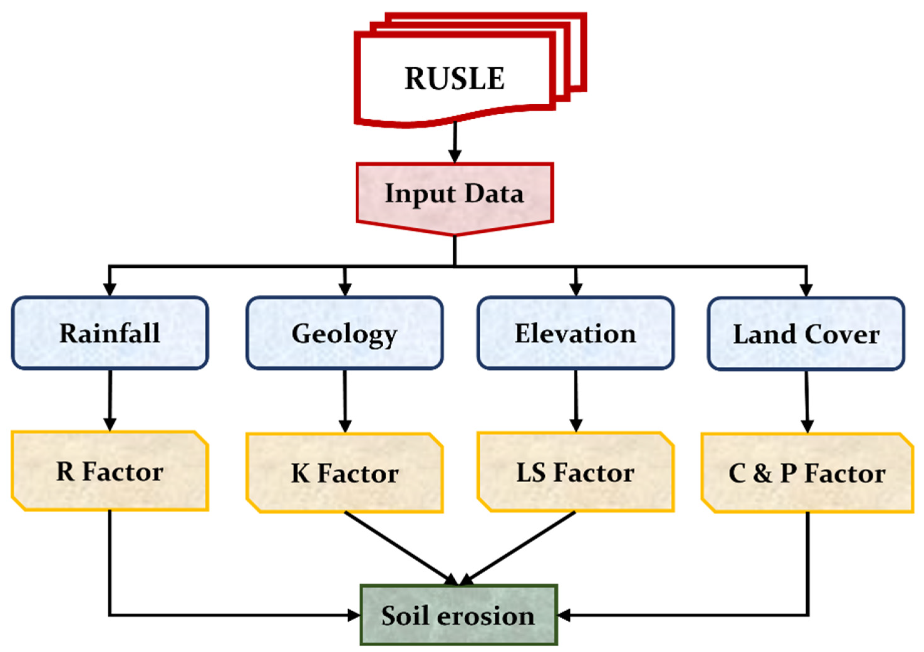
The Revised Universal Soil Loss Equation (RUSLE) is the most widely used model that calculates the rate of soil erosion induced by rainfall and overland flow. The RUSLE model is widely used in Greek territory by researchers, with the necessary adaptations in relation to the various conditions of each research area [5,7,23,24,25,26,27,28,29]. Its ease of use and the ability to define the variables causing water erosion while using highly accessible and accurate data to calculate the average annual soil loss rates in each study area are the elements that have contributed to its widespread adaptation. The factors that contribute to the RUSLE model are the Rainfall-Runoff Erosivity factor (R), the Soil Erodibility factor (K), Slope Length and Steepness factor (LS), Cover Management factor (C), and the Support Practice factor (P).
The accuracy of the input data and the methodologies used to compute each factor have a direct impact on the quality of the final computation. Specifically, the LS factor is of great interest because of the variety of applied equations in the literature to calculate it and the fact that these equations require the use of Digital Elevation Models (DEM). Τhe use of DEM for describing the topography of each research area is a parameter that has a substantial impact on the soil erosion modelling outcomes as the DEM source and resolution determine the accuracy of the derived topographical characteristics like elevation, slope, and slope length [30]. Concerning the definition of the Digital Elevation Model, it is a broad term for describing the digital and mathematical representation of topographic surfaces [31]. In the case where the digital model is referring to the bare ground surface, it is called a Digital Terrain Model (DTM), but if the surface includes any feature above the ground, such as trees and buildings, then it is called a Digital Surface Model (DSM) [32,33].
Many researchers have applied different methodologies for the calculation of the LS factor as well as different types of elevation data like DTMs and DSMs. In 2015, Panagos et al. acquired a 25 m resolution DEM for the estimation of the LS factor for the European Union, indicating that DEM resolution does have a significant impact on the spatial distribution of the LS factor since the increase of DEM resolution contributes to the more accurate representation of the landscape and leads to the improvement of the spatial soil loss calculations [34]. Efthimiou et al., examined the effect of topography on soil erosion by calculating the LS factor using the proposed equations from the USLE and RUSLE models in 8 sub-watersheds in northwestern Greece and pointed out that estimated soil erosion from the two models matches for slopes <20%, but for steeper slopes above 20% soil loss from USLE calculated higher values than RUSLE [35]. Fu et al., used DEM with different grid sizes from 2 to 30 m to calculate the LS factor with the Chinese Soil Loss Equation (CSLE) and concluded that both the average LS factor and soil loss decreased with the increase of the DEM grid size, although the corresponding values from the 10 m and 2 m were similar [36]. Mondal et al., performed an analysis on open source DEM with 30 m resolution and aggregated grid sizes (90, 150, 210, 270, and 330 m) regarding their vertical accuracy and uncertainty in soil erosion estimation using the RUSLE model, indicating that both the accuracy of the elevation data and the estimated soil erosion decrease when the DEM grid size increases [37]. In contrast to the previous studies, Shan et al. used DEM with resolutions from 1 to 90 m and the RUSLE model to examine the effect of resolution on the computations of LS factor and soil erosion in a mountainous area in Australia and suggested that there is an increase in the LS values with the increase of the DEM grid sizes and, more specifically, the L factor increases and the S factor decreases [38]. These opposite results may be linked to the methodology of the LS factor, which did not consider a cutoff factor of the slope length, which would cause the overestimation of the LS factor in areas with long slopes where runoff concentration would produce gullies [39] and to the morphology of the study areas, which were characterized by larger relief regions compared to other studies [40]. In the study of Kruk et al., high-resolution DEM were generated from different methods (aerial photographs, aerial laser scanner, and terrestrial laser scanner) to assess the LS factor and soil erosion using the USLE model, and it was shown that resolution has a significant impact on the LS factor, with the S coefficient strongly affecting the calculation of LS [41]. Lu et al., derived topographic data from five different sources with spatial resolution from 5 to 90 m to assess the LS factor in five catchments in China, and the results indicated that by increasing the grid size, the S factor decreases, the L factor increases, and the overall accuracy of the estimated LS factor is decreased [39]. Wang et al., studied the effect of DEM resolution on the LS factor by implementing two DEM, one derived from Lidar datasets with a 5 m grid size and the other obtained from an SRTM dataset with a 30 m grid size for the computation of LS in 24 watersheds in North America [40]. This study highlighted the increase in the L factor and the decrease in the S factor with coarser DEM resolutions and, regarding the LS factor, the results showed an increase in areas with large relief and a decrease in smaller relief areas. Azizian and Koohi focused on the impact of different source DEM (ALOS, ASTER, SRTM) with different resolutions from 30 to 200 m and produced LS factors with various equations as well as the sediment yield rates in a study area in Iran, concluding that DEM resolution has a more vital role than DEM source and the different methods for the calculation of LS factor [42]. Another study that assessed the impact of DEM from different sources (ASTER, SRTM, and CARTOSAT) and various resolutions from 30 to 250 m was carried out by Pandey et al., who performed the RUSLE model for the Karso watershed in India and displayed the scale dependence of RUSLE [43]. Regarding the effect of DEM resolution, in the above study there is an increase in the calculated mean and maximum LS factor with an increase of the grid size up to 50 and 100 m but for higher grid sizes a corresponding decrease of these values is noticed. Moreover, the impact of the DEM source highlighted the weaker performance of ASTER DEM compared with SRTM and CARTOSAT. Kumar et al., applied the RUSLE model and acquired DEM from SRTM, ALOS, and MERIT with a resolution of 30 and 90 m and compared the calculated soil erosion with observed data, which led to the conclusion that the DEM with a finer resolution (30 m) performed better than the coarser ones (90 m) [44]. Fijałkowska executed a comparative analysis on elevation, slope, L factor, S factor, and total LS factor values using DTMs with various resolutions (1 m to 90 m) and from different sources using the RUSLE model for 3 study areas in Poland, emphasizing the non-uniformity of the change of LS factor with the increase of DTM overall accuracy and concluded that high resolution and accuracy data should be assessed in soil erosion modelling [45].
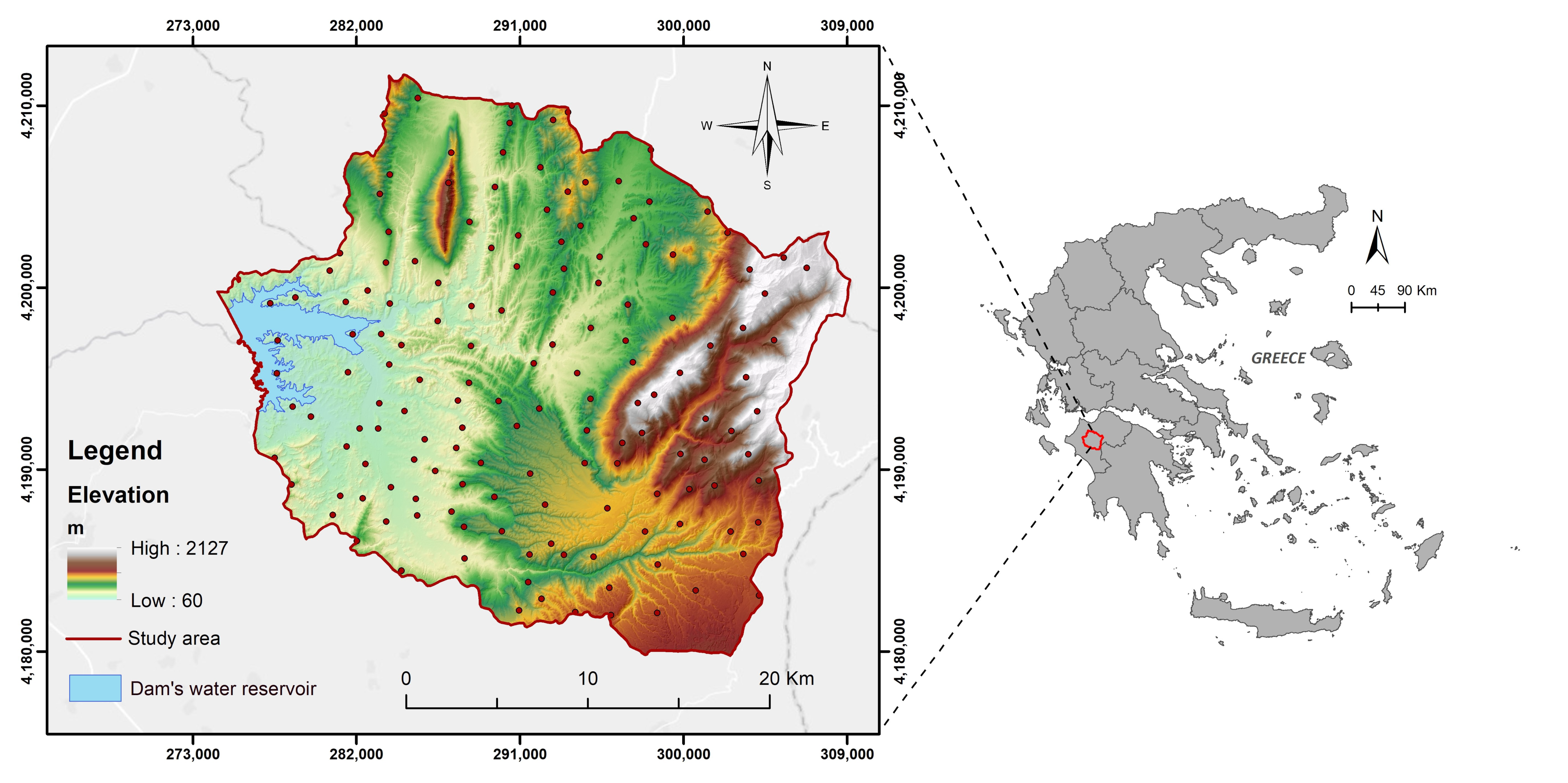
The current study focuses on the importance of topography in soil erosion modelling by examining the impact of topographic data from various sources in the calculation of the slope length and slope steepness factor (LS) of the RUSLE model. It is particularly applied in an area with dense morphology, which has suffered extended surface changes due to repeated wildfires, and this is the drainage basin of the Pinios earth-filled dam located in the Ilia Regional Unit, Western Greece. For the purposes of this study, the topographic data included elevation data from 4 different sources that were compared with Ground Control Points (GCP) to assess their relative vertical accuracy and suitability to produce accurate soil erosion models. Specifically, six Digital Elevation Models with various resolutions and two different methods were applied for the calculation of the LS factor in the examined area. Moreover, for the estimation of the LS factor, the equations proposed by Mitasova et al. [46,47] and the CALSITE (Calibrated Simulation of Transport Erosion) model [48,49] were used.
This research aims to investigate and derive the correlation between DEM and the LS factor, as it is the most crucial parameter of the RUSLE model for estimating soil erosion annual rates. The inspection of the quality of the used DEM in the examined area is of particular interest due to its dense morphology and susceptibility to soil erosion, strongly related to the major wildfires that have affected it for the last fifteen years.
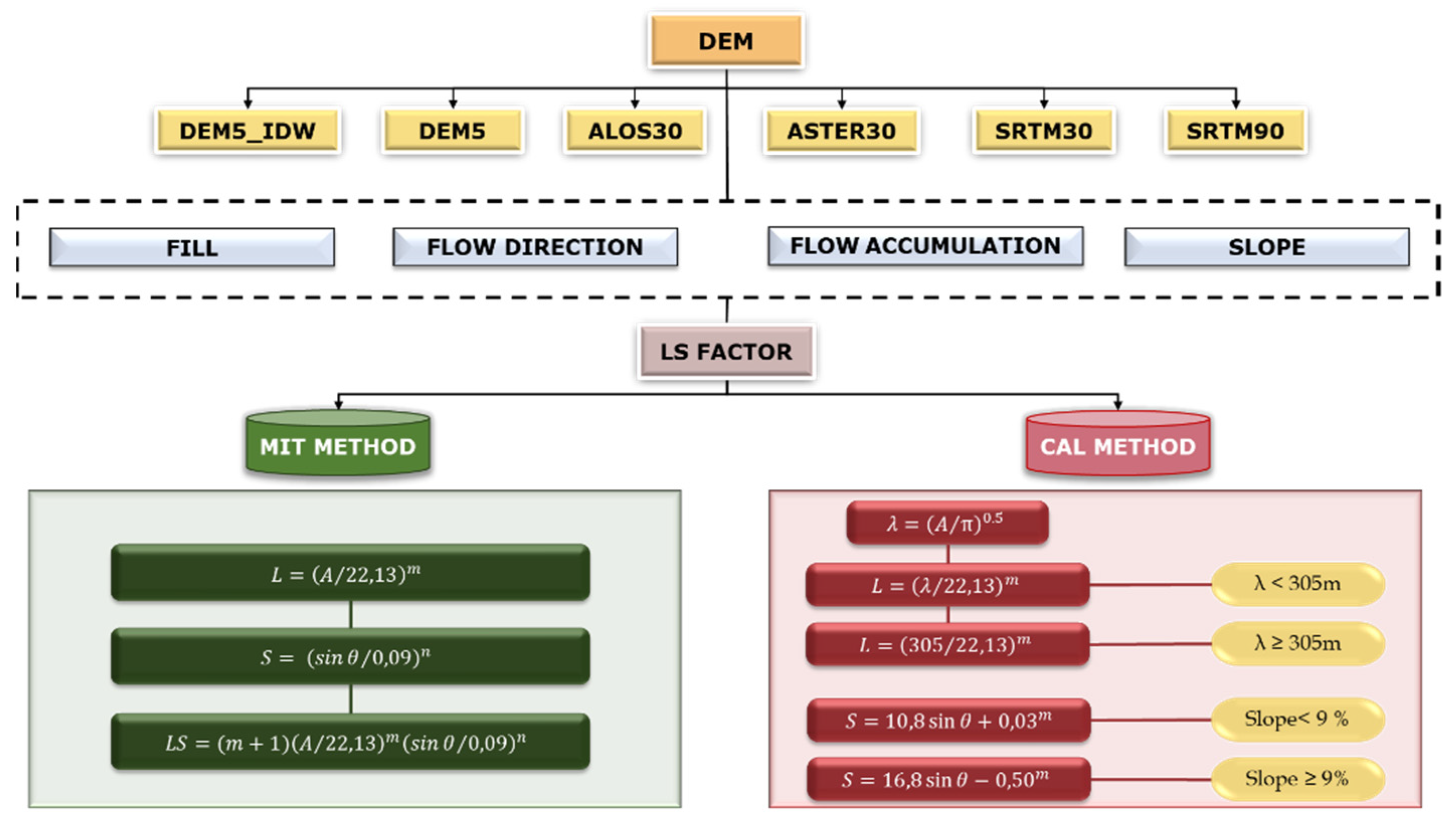
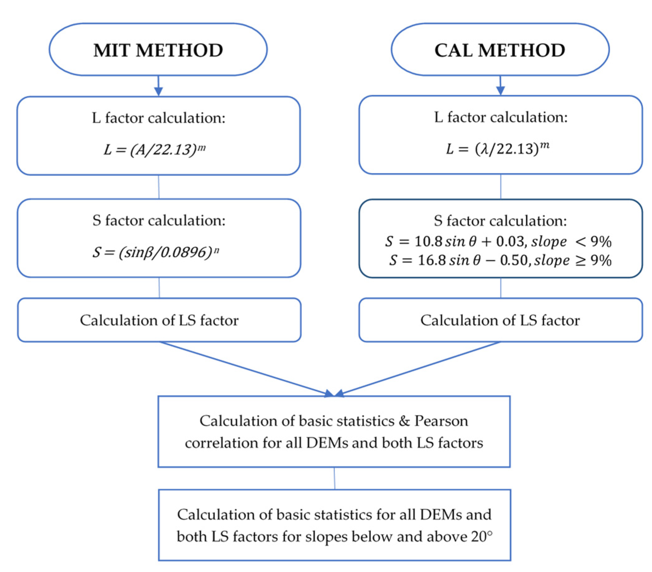
The methodology applied in this research consists of four main stages: (a) the comparison of the examined DEM elevation values with the corresponding values derived from GCP; (b) the comparison of the DEM slope values; (c) the calculation and comparison of the LS factor using two methods, which are referred to as the MIT method [46] and the CAL method [48,49], and (d) the estimation and comparison of the annual soil loss in the pilot area using the RUSLE model and the different calculated LS factors.

2. Research Area and Materials

2.1. Research Area

The drainage basin of the Pinios earth-filled dam, in Western Greece, was selected as a pilot area for this research (Figure 1).
The drainage basin of the dam occupies an area of approximately 700 km2 and the surface water is collected in a large reservoir of approximately 20 km2 [50]. This research area was chosen because of its varied topography, which is of great importance regarding the computation of the LS factor. The altitude ranges from 49 to 2128 m m.a.s.l. and the maximum slope inclination varies from 0 to 80 degrees. According to the Copernicus program “Corine Land Cover 2018”, the pilot area mainly consists of non-irrigated arable land (16%), complex cultivation (11%), land principally occupied by agriculture with significant areas of natural vegetation (25%), sclerophyllous vegetation (14%), and transitional woodland shrub (11%) (Figure 2). Conservation practices like contour farming, cropping, and terraces are mainly occurring in the pilot area.
Subsequently, the land cover data of the 2018 version of the European Corine Land Cover (CLC) were obtained from the Copernicus Land Monitoring Services program [51] for the calculation of the cover management factor (C) of the RUSLE model.
Regarding the climate conditions, the research area is strongly influenced by the Mediterranean Sea, presenting typical Mediterranean climate conditions with high mean monthly temperature values (20–25 °C) during the summer and significantly lower values in the winter (4–10 °C) [52]. Daily precipitation data from six meteorological stations located in the Pinios Dam drainage basin were processed from 1977 to 2020. The mean annual precipitation values range approximately from 660 to 1482 mm. The higher values are present in the mountainous areas (eastern part), while lower values are evident in the western part in areas with small relief. The mean annual precipitation value for the pilot area is equal to 920 m (Figure 3). The rainfall data were also processed for the calculation of the rainfall-runoff factor (R) used in the RUSLE model.
The geological formations prevailing in the research area are mainly Quaternary deposits and Neogene sediments that overlay the Alpine formations from the Greek Geotectonic zones of the Ionian, Gavrovo-Tropolitsa, and Olonos-Pindos, which shape the area around the Pinios dam drainage basin. Fine-grained, coarse-grained and mixed soils are evident mainly in the Quaternary and sediment deposits. The geological setting was designed from four geological sheets (scale 1:50.000) of the Hellenic Survey of Geological and Mineral Exploration to estimate the soil erodibility corresponding to the (K) factor of the RUSLE model. The following figure presents the geological formations in the research area (Figure 4).

2.2. Elevation Data

The elevation datasets acquired for this study were chosen according to their availability and their spatial resolution. They include DEM files which were derived from different sources (satellite missions and aerial photos), reflecting different production technologies and different types of processing.
The descriptive information about the DEM data that was used is reported in the following sections and Table 1.
  • Hellenic Cadastre DEM: «DEM5».
The Hellenic Cadastre produced a DTM that covers the entire region of Greek territory with a pixel size equal to 5 m and high vertical accuracy of approximately 2 m. The DEM data series is part of the Large Scale Orthophotos (LSO) project implemented during the period 2007 to 2009. The aerial photos captured by a digital onboard camera were used as the source data for producing the relevant DTMs.
2.
ALOS World 3D-30 m (AW3D30) v3.1, Global Digital Surface Model: «ALOS30».
Five years ago, JAXA freely offered to the research community a Digital Surface Model with almost global coverage [61]. Since then, new updates have been released [62]. The specific DSM is created from millions of images acquired by the ALOS PRISM sensor with automatic procedures and without the use of GCP. According to the specifications and diverse studies, both the planimetric and vertical accuracy should not exceed 5 m [63,64]. In a recent study by Nikolakopoulos (2020) for seven areas in Greece, the mean RMSE was measured at 8.58 m [33]. It is also proven that the error increases in mountainous or steep areas and urban centres. Similar results were also presented in the study of Stamatiou et al., with the calculated RMSE value being equal to 8.75 m for the Greek territory [65].
3.
ASTER GDEM Version 3 «ASTER30».
The initial version of ASTER GDEM was launched in 2009, followed by Version 2 in 2011, and Version 3 in 2019. It was created from the automated processing of 2.3 million scenes from the ASTER archive, which were acquired during the period from 2000 to 2013. With a 30-m spatial resolution and 1° × 1° tiles, the ASTER GDEM Version 3 preserves the GeoTIFF format and the same gridding and tile structure as earlier versions [66,67]. The stereo pairs were reprocessed thoroughly, and the tiles were manually inspected and corrected for any abnormalities, minimizing the errors in this data collection. Any holes in this dataset were filled either from other data like SRTM and national data sets, or by using interpolation techniques, or by leaving them blank [68]. Regarding the vertical accuracy of ASTER DEM data in Greek territory, studies have shown RMSE values to be approximately equal to 10 m [68,69].
4.
SRTM DEM Version 3 «SRTM30 & SRTM90».
The major purpose of the SRTM Version 3 dataset was to remove voids that existed in previous SRTM data releases. Existing topographical data were utilized to enhance the SRTM data in regions where there was a lack of data. The filling of holes in the Version 3.0 products using the ASTER Global Digital Elevation Model (GDEM) Version 2.0, the Global Multi-resolution Terrain Elevation Data 2010 (GMTED2010), and the National Elevation Dataset (NED) are among the enhancements over earlier versions. This SRTM Version 3 dataset, which comprises the worldwide 1 arc-second (30 m) product and the global 3 arc-second (90 m) product, is maintained and distributed by the Land Processes Distributed Active Archive Center (LP DAAC). Using averaging methods, the 3 arc-second data was extracted from the 1 arc second data [59]. The vertical accuracy of SRTM data in Greek territory was found to be equal to 6.1 m [69] and 6.9 m [69].

3. Methodology

The methodology applied in this research could be divided into 4 main sectors: (1) DEM analysis and comparison with the respective GCP to examine the quality of each DEM and its adequacy with soil erosion modelling; (2) comparison of the values of the slopes derived from each DEM; (3) calculation of the LS factor by using the DEM and two methods, which are the method suggested by Mitasova et al. (MIT method) [46] and the method explained by the CALSITE model (CAL method) [48,49] to examine the differences of the LS when using diverse approaches and DEM with various resolutions; and (4) estimation of the annual soil erosion rate using the RUSLE model according to the methodology applied by Depountis et al. [24].

3.1. DEM Quality Assessment

The Digital Elevation Models used in this research were derived from different sources (satellite missions and aerial photos) and evaluated regarding their relative vertical accuracy for the pilot area according to the methodology presented in Figure 5.
The initial processing of the elevation data files includes the conversion of the original projection system to the Greek Geodetic Reference System (GGRS87), the creation of a mosaic from the individual tiff files, and the clipping according to the research area boundaries. Regarding the vertical accuracy assessment, it is noted that most of the examined Digital Elevation Models are specifically Digital Surface Models which correspond to elevation data that include not only the ground surface but everything above it, such as the heights of tree canopy and engineering constructions. To suppress this issue, the accuracy assessment was performed with the use of Ground Control Points from the National Trigonometric Network, which is operated by the Hellenic Army Geographical Service (HAGS). These points are always located in flat places providing easy access, meaning that, for this study, they are suitable for performing the vertical accuracy assessment [33]. Thus, the elevation value of each GCP was compared with the corresponding value of each DEM for these particular points.
The ArcGIS Spatial Analyst toolbox was used to extract altitude values from the DEM for each checkpoint. The purpose of this procedure was to compare the elevation value of the DEM with that of the trigonometric points to calculate their deviation. Specifically, the option “Bilinear interpolation of values at point location” is preferred because it gives value to the point through linear interpolation and not from the centre of the pixel. After the data extraction, an error check was performed to remove points that were not suitable or were located near the research area’s boundaries. The exclusion of extreme values (outliers) was based on the application of a threshold value resulting from the calculation of a certain accuracy indicator. For the error check, Root Mean Square Error (RMSE) was selected as the accuracy index. The values of the points to which the relation Δhi> 3 * RMSE applies were defined as error outliers [70,71]. In the end, 150 points were used to evaluate the altitude information of the DEM. Of these 150 points, 112 (75%) were used to correct the DEM that was derived from the Hellenic Cadastre, while the remaining 38 points (25%) were used to validate the newly corrected DEM (validation points). For each one of the 112 trigonometric points, the error was calculated, i.e., the difference between the altitude value of the DEM and the trigonometric point, and then the spatial distribution of this difference was performed by using the IDW (Inverse Distance Weighting) method. Moreover, the raster file containing the error was added using the map algebra toolkit and the raster calculator tool to the DEM of the Hellenic Cadastre. This process was executed to create a new DEM which is more reliable in terms of its vertical accuracy [72,73]. This is supported by the calculation of the RMSE values for the 38 validation points for both the original DEM from the Hellenic Cadastre and the corrected one. The RMSE value for the original was calculated to be equal to 1.666 m, so the corresponding value for the new one is equal to 1.096 m.
Regarding the impact of DEM resolution on the LS factor, a statistical analysis of the DEM elevation values was applied along with a vertical accuracy assessment with the use of GCP, which are considered to be more accurate compared with the DEM values. Subsequently, the elevation value of each GCP was compared with the corresponding value of each DEM in the research area. For this purpose, the difference between the GCP and DEM values was used, which is the vertical error (Δh) = h DEM − h GCP [32,33,68,72,73,74].
Within the context of the DEM vertical accuracy assessment, the descriptive statistics of each DEM and the Pearson correlation coefficient were calculated [75]. Afterwards, both of them were calculated for the error (Δh), which corresponds to the subtraction of the elevation value of the DEM and the corresponding value of the check point for each one of the 150 points. Regarding the evaluation of the errors, the calculation of more adequate accuracy metrics was considered appropriate for this article. Specifically, the Mean Absolute Error (MAE), the Mean Squared Error (MSE), the Root Mean Square Error (RMSE), the symmetric Mean Absolute Percentage Error (sMAPE), the Median Absolute Deviation (MAD) and the Normalized Median Absolute Deviation (NMAD) were calculated and their histograms for different height intervals were examined. The MAE, MSE, and RMSE are scale-dependent measures. The sMAPE is a scale-independent accuracy metric based on the percentage or relative error, with a lower and an upper bound, that may be used to compare the accuracy of the forecasted elevation values [76]. The RMSE is the most widely applied index for vertical accuracy assessment [33,72,73,77,78,79]. Furthermore, as a part of the descriptive statistics, skewness and kurtosis (excess) were also calculated to examine the normality of the errors. According to Höhle and Höhle, the median is a robust estimator for a systematic shift of the DEM and is very useful because it is less sensitive to outliers in the data than the mean error and also provides a better distributional summary for skew distributions [70,80]. Taking that into consideration, the robust statistical indexes (Table 2), the MAD and NMAD [70], were calculated for the vertical accuracy assessment of the DEM elevation values [68,78,81,82,83].
The Median Absolute Deviation (MAD) is the 50th percentile of the absolute values of the errors. The Normalized Median Absolute Deviation (NMAD) is obtained by multiplying MAD by the factor 1.4826. The NMAD is another robust accuracy metric that calculates the vertical error distribution scale. It may be conceived as an estimate of the standard deviation which is more resistant to the outliers in the dataset. According to Jacobsen, the differences between a DEM and the reference data used for the vertical accuracy assessment (Δhi) do not always follow a normal distribution, which leads to larger discrepancies between these two statistical indicators [84]. In the case of normal data distribution, NMAD is equal to the standard deviation, but only if the number of the examined checkpoints is quite large [70]. The robust metrics are important quality measures when there is a significant deviation between mean and median or standard deviation and normalized median absolute deviation [31].

3.2. Calculation of LS Factor

Two of the most important parameters that affect soil loss are the slope (S), which affects both rainfall-runoff erosivity and the rate of the detachment of soil particles from the rain drops, and the length of the slope (L), i.e., the length of the surface flow until it reaches a natural or artificial recipient [85]. The slope-length factor (L) and the slope gradient factor (S) should be considered as a single topographic factor (LS) in the soil loss equation [86]. The slope-length factor (L) is the ratio of soil loss (A) from a field slope length (λ) to that from a slope 22.13 m long (Equation (1)), and it measures the distance from the origin of overland flow along the flow path to the location of deposition. The slope-steepness factor (S) is the ratio of soil erosion from the field slope gradient to that from a 9% slope. The slope-steepness factor (S) is the ratio of soil erosion from the field slope gradient to that from a 9% slope (Equation (2)) [18].
L = λ 22.13 m
where λ is the slope length (m) and m is an empirical coefficient (dimensionless).
S = sin θ 0.0896 n
where θ is the angle of the slope (°) and n is an empirical coefficient (dimensionless).
According to the above equations, L and S factors are calculated by slope length and slope angle. Slope length (λ) is the distance from the point of origin of overland flow to either of the following: (a) the point where the slope decreases to the extent that deposition begins, or (b) the point where runoff enters a well-defined channel that may be part of a drainage network or a constructed channel [18]. The slope length is the horizontal projection, not the distance parallel to the soil surface [87]. Field measurements are the best approach to assessing slope length, but they are rarely available or practical. According to Barriuso Mediavilla et al., there are some basic principles to consider in order to produce a comprehensive approach for calculating the LS factor [88]. These are the global methods to calculate L and S factors, the procedure to estimate slope length (λ), the method to estimate the empirical coefficients and several other considerations for the hydrological network and water bodies.
The role of Digital Elevation Models (DEM) in soil erosion analysis is vital as they are utilized for the estimation of LS factor, usually at the catchment scale, meaning that the calculated LS values are highly dependent on the DEM accuracy and source [39,89,90]. In this research, two approaches were selected for the calculation of the LS factor, the equation suggested by Mitasova et al. (MIT method) [46,47] and the one from the CALSITE model (CAL method) [48,49]. The selected DEM as well as the above formulas were imported into the ArcMap software to estimate the distribution of the LS factor according to the following flowchart (Figure 6).

3.2.1. The MIT Method

The LS factor is generally estimated by applying the equations by Moore and Burch and Moore & Wilson Equation (3) [91,92,93]:
L S = A / 22.13 m   sin β / 0.0896 n
where A is a specific catchment area (m2/m), β is the slope angle in degrees, m is equal to 0.4 for Moore and Burch approach [91] or 0.6 for Moore and Wilson approach [92], n is equal to 1.3 and the values 22.13 (m) and 0.0896 (sin5.143°) are referring to the length and slope of the standard unit plot. This equation was later adjusted by Moore et al. [93] by multiplying the equation with the value 1.4 and was applied by Van der Kniff et al. for Europe (Equation (8)). Subsequently, Mitasova et al. modified the previous version by replacing the hillslope length with the upslope contributing area [47], as follows (Equation (4)) [46,94]:
L S = m + 1 A / 22.13 m   sin β / 0.0896 n
where A is a specific catchment area (m2/m), β is the slope angle in degrees, m is equal to 0.4–0.6, n is equal to 1.0–1.3, and the values 22.13 (m) and 0.0896 (sin5.143°) refer to the length and slope of the standard unit plot.
According to Mitasova and Mitas, the replacement of slope length used in the original formulation of USLE/RUSLE with the upslope area provides a better spatial description of increased erosion due to the concentrated flow without the need to a priori define these locations as inputs for the model [46].

3.2.2. The CAL Method

In the GIS framework, flow accumulation is used for the estimation of slope length by the multiplication of flow accumulation with the DEM resolution. According to Barriuso Mediavialla et al., this method is not suitable because the flow accumulation is added at every convergence [89]. This issue has been addressed by another method that uses the slope length for LS calculation, as suggested by the CALSITE model (Calibrated Simulation of Transport Erosion) [95]. This model contemplates flow accumulation areas (cells) as in a circle, meaning that to calculate slope length in a specific cell, we consider the flow accumulation area in that particular cell as if it was a circle, which indicates that the distance travelled by a single water drop is equivalent to its radius [48,88]. The suggested equation included in CALSITE considers the spatial distribution of λ and has the following form (Equation (5)):
λ = A π 0.5
where λ is the slope length, A is the upstream contribution area and π is the value of 3.1416.
An appropriate upper threshold was determined to deal with the issue of too high slope length values calculated from the above equation. According to Renard et al., runoff erosion is usually concentrated in less than 121.92 m length, although lengths of up to 304.80 m have been observed [87]. In 2019, Schmidt et al. proposed the application of a 100 m slope length threshold based on experiments in alpine environments [96]. McCool et al. and Winchell et al. mention that an upper limit of 333 m should be applied for slope length [97,98]. For this research, this upper threshold value of slope length was set to be equal to 305 m as proposed by the studies of Renard et al. and Kang & Julien [88,96]. This threshold for slope length (λ) is implemented in the above equation to define the upper flow accumulation threshold value for each DEM, meaning that if a cell value outreaches this flow accumulation value, then its slope length will be set to be equal to 305 m. This approach changes the slope length equation as follows (Equation (6)):
L = λ 22.13 m ,   f o r   f l o w   a c c u m u l a t i o n t h r e s h o l d   v a l u e   d e p e n d a n t   o n   D E M   r e s o l u t i o n 305 22.13 m , f o r   f l o w   a c c u m u l a t i o n > t h r e s h o l d   v a l u e   d e p e n d a n t   o n   D E M   r e s o l u t i o n  
Additionally, a lower threshold value must be specified such that the cells indicating ridges (cells higher than any of the eight around them) have values other than zero. This procedure aims at the separation of these cells from the cells indicating streams and water bodies which also have zero values. According to Barriuso Mediavilla et al., these cells travel a distance of half a cell, so their flow accumulation value is set to 0.5 as the lower threshold value of flow accumulation [88]. It is predicated on the notion that slope length estimates are measured from the cell’s centre [95].
According to Renard et al., soil loss increases more rapidly with slope steepness compared with slope length [87], which highlights the importance of the S factor. The CALSITE model uses the equations of McCool et al., for the calculation of the S factor (Equation (7)) [99]:
  S = 10.8 sin θ + 0.03   f o r   s l o p e   s t e e p n e s s < 9 %   5.14 °   o r   S = 16.8 sin θ 0.50   f o r   s l o p e   s t e e p n e s s 9 %   5.14 °
The slope-length exponent m is related to the ratio ß of rill erosion (caused by flow) to interrill erosion (principally caused by raindrop impact) by the following equation (Equation (8)) [100]:
m = β / 1 + β
Values for the ratio β of rill to interrill erosion for conditions when the soil is moderately susceptible to both rill and interrill erosion were computed by McCool et al. with the use of the following equation (Equation (9)) [101]:
β = sin θ / 0.0896 /   3 s i n θ 0.8 + 0.56
where β is the rill to interrill ratio and θ is the slope angle.

3.3. Annual Soil Loss

The estimation of the annual soil erosion rate is performed by applying the RUSLE model (Figure 7) in the study area, which is based on previous research by Depountis et.al., [24]. Specifically, the modified Fournier index [102] and the equations of Renard and Freimund [103] were used for the calculation of the R factor, and the methodology of Wischmeier and Smith was applied for the K factor [18,86]. The Corine Land Cover database (CLC) was used for the estimation of the C factor, and each land use category from CLC was matched with a corresponding bibliographic value. Lastly, the P factor was set to be equal to 0.5 considering that nearly 50% of the total area is devoted to agricultural areas implementing the support practices in the research area. The P factor is the most ambiguous since it was based on the CLC database and field observations.
The computed average soil loss per unit area (SE) is expressed in tones/ha/year, the rainfall-runoff erosivity factor (R) is expressed in MJ·mm·ha−1·h−1·year−1, the soil erodibility factor (K) is expressed in t·h·MJ−1·mm−1. The slope length factor (L), the slope steepness factor (S), the cover management factor (C), and the erosion support practice factor (P) are dimensionless.

4. Results

4.1. DEM Comparison

The first stage of the DEM quality assessment includes the calculation of the descriptive statistics (min, max, mean, standard deviation, range (min-max)) for each DEM as presented in Table 3.
According to the above statistical analysis, the elevation values from each examined DEM have a substantial degree of similarity. The similarity of the DEM elevation values is evident even though the DEM vary regarding their resolution and source. This is supported by high Pearson correlation values (Appendix A: Figure A3a) that were calculated for every pair of DEM as the lowest coefficient value was noted between SRTM90 and ALOS30 and is equal to 0.99470.
The second stage of the quality assessment includes the examination of the vertical accuracy of each DEM. This is accomplished by comparing the elevation values of the DEM with the corresponding elevation values of 150 ground control points, which are considered to be more accurate. The descriptive statistics of the error (Δh) are presented in Table 4.
The mean error (Δh) values do not follow the similarity pattern of the elevation values. The interpretation of the histogram errors (Appendix A: Figure A1) concurrently with the examination of the descriptive statistics shows that DEM5 and the corrected DEM5_IDW are substantially better than the other DEM with mean values of 0.2 and −1.15 and a standard deviation of 0.54 and 1.39. Following that, ALOS30 and SRTM30 appear to have a similar mean (−7.77 and −10.63) and standard deviation values (4.47 and 4.84). Subsequently, ASTER30 and SRTM90 have resembling mean (−15.62 and −18.28) and standard deviation (9.51 and 8.18) values and seem to be the most inadequate out of the six examined DEM.
Except for the basic statistics that were reported above, more adequate measurements were performed with the calculation of the MAE, MSE, RMSE, and sMAPE (see Table 2). Skewness and kurtosis (excess) were also calculated as part of the descriptive statistics showing the non-normality of the errors (see Appendix A: Figure A1), which led to the decision to calculate the two more robust statistical indexes, the MAD and NMAD (see Table 2), for the vertical accuracy evaluation of the DEM elevation values (Table 5).
Regarding the calculated accuracy metrics MAE, MSE, RMSE and sMAPE, the DEM5 and the corrected DEM5_IDW have the lowest values. Following, ALOS30 and SRTM30 have similar values but are quite higher compared to DEM5 and DEM5_IDW. Likewise, ASTER30 and SRTM90 have resembling values and are the highest of all the examined DEM (sequence from lowest to highest: DEM5_IDW, DEM5, ALOS30, SRTM30, ASTER30, SRTM90). The same observations seem to appear for the robust metrics, with the exception that ASTER30 has the highest MAD and NMAD values (sequence from lowest to highest: DEM5_IDW, DEM5, ALOS30, SRTM30, SRTM90, ASTER30). According to all the above statistical measures, DEM5 and DEM5_IDW appear to be the most accurate, with ALOS30 and SRTM30 following, and lastly, ASTER 30, and SRTM90 seem to have the highest divergence from the reference elevation data of the ground control points. Additionally, histograms of the statistical indexes mentioned above were made according to the height intervals <500 m, 500–1000 m and >1000 m for each DEM, showing that the errors are increased in high elevations that exceed 1000 m for all DEM (see Appendix A: Figure A2).

4.2. Slope Values Comparison

The comparison of DEM with different cell sizes may provide some important information regarding the accuracy of these elevation data, but that is not the case for DEM derivative files such as slope [32]. A comparison of different DEM files might show quite similar elevation values, but the corresponding slope values will vary a lot more. Slopes could be produced from DEM using different algorithms that affect the final result too [104,105,106,107,108,109]. In this study, the slope angle for each grid cell is calculated using a specific numerical method known as the Deterministic-8 or D-8 method in ArcGIS 10.8. A moving 3 × 3 window is used to examine the DEM matrix, and the four grid cells nearest to the centre cell are twice as weighted as the four grid cells diagonally across the centre cell [110].
Unlike the previous comparisons of DEM elevation data, the slope value comparison from the 6 DEM shows high divergence. The descriptive statistics (min, max, mean, standard deviation, range (min-max)) for the calculated slopes of each DEM are presented in Table 6.
The minimum slope value is zero for all the DEM data. The maximum slope value is noted in the Hellenic Cadastre DEM (DEM5) and the corrected DEM5_IDW and is equal to 86° approximately. The maximum slope values for the other DEM decrease with the increase of cell size, meaning that the higher the DEM resolution, the higher the maximum calculated slope value, which is supported by the fact that the slope was calculated with the D-8 method, meaning that it is based on 8 neighbour cells, making the slope sensitive to any resolution alterations [111]. This is also evident in the slope values of standard deviation, mean, and median, but from comparing the mean and median for all DEM it appears that they do not vary so much, ranging from 12.34 to 19.05 and 9.08 to 17.05, respectively. Another important factor is the type of DEM from which the slope was calculated. The DEM5 and the corrected DEM5_IDW are DTMs in contrast to the other used DEM which are DSMs. According to Polidori and Simonetto who compared one DTM and one DSM in the Amazonian landscape, it was shown that calculating slope from DSM rather than DTM resulted in an error of 5° for 30 m and 2° for 90 m spatial resolution DSMs [112].
As mentioned before, the Pearson correlation coefficients for the elevation values in the DEM are very high and do not fall below 0.99. On the contrary, Pearson correlation coefficients for the slope values of each DEM appear to be significantly lower (Appendix A: Figure A3b). Slopes calculated from the DEM5 and the DEM5_IDW have the highest Pearson correlation value equal to 0.98727, while the lowest value belongs to the pair DEM5_IDW-SRTM90 and is equal to 0.66051.

4.3. LS Factors Comparison

Two different approaches were used to examine the impact of the LS factor in soil loss results obtained by the RUSLE model. The first one is based on the equation that was suggested by Mitasova et al. (MIT method) [46,47] and the second one utilizes the equation from CALSITE model (CAL method) [48,49] (Figure 8).
The greatest difference between these two methods is related to the L factor calculation. The first method uses the upslope area (A) and the second one the slope length (λ) posing an upper threshold value equal to 305 m which is implemented in λ equation to define an upper flow accumulation threshold value for each DEM. The other significant difference concerns the S factor and relies on the fact that the CALSITE method uses the equations of McCool et al. [100] which consider the percentage of slope steepness, setting a threshold of 9% (or 5.14 degrees). Subsequently, twelve maps of LS factors were generated using the two methods for each of the six DEM. The results are presented in Appendix B where Figure A4 shows the LS factor for DEM5, DEM5_IDW and ALOS30 while Figure A5 shows the LS factor for ASTER30, SRTM30 and SRTM90.
The descriptive statistics were calculated for the LS factors for each approach and DEM. LS factor values calculated using the MIT method show significantly high maximum values reaching 7980.78 for DEM5_IDW and 7975.30 for DEM5 while the lowest maximum value equal to 927.58 is presented by SRTM90 (Table 7).
In this case, it is evident that the higher the resolution of the DEM data, the higher the maximum LS values. This observation, though, does not apply to mean values. The lowest mean value falls below 10 and is calculated in SRTM30 equal to 8.77 and the highest is calculated in ALOS30 equal to 11.41 followed by SRTM90 with 10.97, DEM5_IDW and DEM5 with 10.68 and lastly, ASTER30 with 10.12.
LS factor values calculated using the CAL method (CALSITE model) show significantly lower maximum values compared to the corresponding ones from the MIT method (Table 8).
Specifically, the highest maximum value was calculated in DEM5 and DEM5_IDW equal to 42.87 and the lowest in ASTER30 equivalent to 33.71 m. The statement that the higher the resolution of the DEM data, the higher the maximum LS values, is partially correct for this method as a decrease in maximum values with the decrease of DEM resolution is observed, excluding the SRTM90 value, which is surprisingly higher than expected. In the case of mean values, DEM5 and DEM5_IDW with 3.24 present the lowest mean value, while SRTM90 has the highest mean value equal to 5.08.
The following figure shows the difference between the calculated mean values of LS factors using both of the examined approaches (Figure 9). It is noticeable that mean LS values from the MIT method are much higher compared to the CAL method for all the DEM data. The lowest mean LS for the CAL method is calculated from the DEM data with the lowest pixel size, which is 5 m (DEM5 & DEM5_IDW) while the highest mean value is calculated from the DEM with the highest pixel size equal to 90 m (SRTM90). This is not evident in the MIT method as the lowest mean LS value, in this case, was calculated from the SRTM30 and the highest from ALOS30.
Apart from the descriptive statistics of the LS factor, the Pearson correlation coefficient was also estimated for the MIT method and each DEM (Appendix A: Figure A3c). The examination of this coefficient shows a significant divergence of LS values for all the DEM pairs except for DEM5 and the corrected DEM5_IDW which have the highest Pearson correlation coefficient value equal to 0.98284, approximately. For the other pairs, the correlation values fall under 0.40.
Pearson correlation coefficient values for LS factor calculated with the second method (CAL) are presented in Appendix A: Figure A3d. The similarity of LS values with the first method was considerably low. On the contrary, Pearson correlation values for LS values of the CALSITE model are notably higher, showing greater similarity. The highest value is calculated between the DEM5 and the corrected DEM5_IDW and is equal to 0.99864. The lowest value was calculated between ASTER30-DEM5_IDW equal to 0.61338. Notably, the lowest Pearson correlation coefficient value of this method is greatly higher than the corresponding one of the first method which is equal to 0.15257.
In order to examine the effect of slope in the LS factor, the same statistics were calculated for two cases, the first one for slope values below 20° and the second one for slope values above 20°. The threshold of 20° was chosen considering that slope values above that are considered significantly high and the fact that the highest mean slope value (from DEM5 and DEM5_IDW) was calculated to be almost 20° (19.05°).
The LS factor calculated for areas with slope values below 20° shows significantly lower mean and maximum values compared to slopes higher than 20°. This is evident from the LS factor estimated with both the examined methods. For the MIT method, the max values tend to decrease with the increase of the pixel size of the DEM. The opposite from that is occurring for the mean values which tend to increase when the DEM resolution gets lower (Figure 10).
The LS values from the CAL method display different behaviour with the DEM resolution changes for slopes below 20°. The maximum values are almost identical while the mean values tend to increase with the increase of pixel size. For slopes above 20°, the maximum values decrease while the mean values increase with lower resolution (Figure 11).

4.4. Annual Soil Loss Comparison

Annual soil loss of the research area was estimated by acquiring the Revised Universal Soil Loss Equation and multiplying the Rainfall-Runoff Erosivity Factor (R), Soil Erodibility Factor (K), Slope Length and Steepness Factor (LS), Cover Management Factor (C) and Support Practice Factor (P). A similar estimation for this particular area, except for the LS factor, has been presented by Depountis et al. [24]. The topographic factor LS was calculated twice based on two different approaches; hence, soil erosion rates were estimated twice for each one of the examined DEM. Subsequently, twelve maps of soil erosion were produced using the RUSLE model with the LS factors estimated with the MIT and CAL methods for each of the six DEM. The results are presented in Appendix B where Figure A7 presents soil erosion for DEM5, DEM5_IDW and ALOS30 while Figure A6 presents soil erosion for ASTER30, SRTM30 and SRTM90.
The obtained results of this procedure are presented in tables showing the descriptive statistics min, max, mean, standard deviation, and range (min–max) of the estimated soil erosion rates (SE) for every DEM and LS. Regarding the soil loss estimated with the LS factor derived from the equation of Mitasova et al. [46,47], extremely high maximum values are observed, reaching the value of 261,063.14 ton/ha/year in DEM5_IDW. The lowest maximum value is presented in SRTM90 and is equal to 19,865.85 ton/ha/year. The corresponding mean values are almost reaching 100 ton/ha/year with the highest presented by ALOS30 and SRTM90 equal to 98.62 and 98.43 ton/ha/year respectively. The lowest mean value belongs to SRTM30 with 75.47 ton/ha/year (Table 9).
Again, the Pearson correlation coefficient was estimated for each DEM (Appendix A: Figure A3e). The examination of this coefficient shows a substantial divergence of SE values for all the DEM pairs except for DEM5 and the corrected DEM5_IDW which have the highest Pearson correlation coefficient value equal to 0.98225 followed by the pair SRTM30-ALOS30 with 0.37296. The lowest value was calculated between ASTER30-DEM5_IDW and ASTER30-DEM5 equal to 0.08961 and 0.08917.
Regarding the soil erosion (SE) estimated with the LS factor derived from the equation of the CALSITE model, the highest calculated maximum value is 1637.18 ton/ha/year and belongs to DEM5 and DEM5_IDW. The lowest maximum value is calculated in SRTM90 and is equal to 1040.39 ton/ha/year. The corresponding mean values do not exceed 50 ton/ha/year with the highest presented by SRTM90 and ALOS30 equal to 42.51 and 40.27 ton/ha/year. The lowest mean value belongs to both DEM5 and DEM5_IDW and is equivalent to 28.78 ton/ha/year (Table 10).
As for the Pearson correlation coefficient of soil erosion (SE) calculated with the second LS factor method for each DEM, it is highly noticeable that there is less divergence compared to the corresponding results of the first method. Specifically, the highest value belongs to the DEM5-DEM5_IDW pair, equal to 0.99914, followed by the pair SRTM30-ALOS30 with 0.86739. The lowest value was calculated between SRTM90-DEM5_IDW and SRTM90-DEM5, which were equal to 0.57054 and 0.57061 (Appendix A: Figure A3f). As a result, the mean SE annual rates calculated for each DEM using the CAL method are considerably lower than the relevant SE values calculated using the MIT method (Figure 12).
The descriptive statistics of soil erosion (SE) were also calculated for slopes below and above 20°. The SE values calculated in areas with slopes below 20° show considerably lower mean and maximum values compared to the values calculated for slopes above 20° for both the MIT and CAL method scenarios. Particularly for the MIT method and for both cases (above and below 20°), the maximum values present a decreasing tendency as the DEM resolution is getting lower. Conversely, the opposite tendency is occurring for the mean values as they increase when the DEM resolution gets lower (Figure 13).
Regarding the CAL method, the mean and max values for slopes above 20° are significantly higher than the calculated ones for slopes below 20 degrees. For both cases (above and below 20°), the maximum values tend to decrease while the mean values increase as the DEM resolution is getting lower, following the same pattern as the values from the MIT method. (Figure 14).

5. Discussion

The evaluation of role of topography in soil erosion modelling was assessed by examining the impact of elevation data from various sources on the slope length and slope steepness factor (LS) estimation. Specifically, 6 Digital Elevation Models (DEM) were acquired from 4 different sources and then compared with ground control points (GCP) to analyze their relative vertical accuracy and evaluate them in terms of their suitability for soil erosion model production. The DEM had various resolutions and were used to calculate the LS factor with two different equations. The RUSLE model was then used to estimate the annual soil erosion rates for each one of the examined approaches and DEM. Regarding the soil loss estimation with the RUSLE model, it is noted that all the parameters (R, K, C, and P) remained constant, except for the LS factor, which was calculated by applying two different equations, meaning that any variations in estimated soil loss values for each DEM are caused by the LS factor.
The quality of the final computations of the LS factor, and subsequently the annual soil erosion rates, directly depends on the accuracy of the input data and the calculation techniques utilized for each factor of the RUSLE model. In particular, the LS factor is very important because of the variety of equations used in literature for its estimation and the fact that it requires the application of DEM data. The accuracy of the DEM-generated topographical characteristics, such as elevation, slope, and slope length, is determined by the DEM source and resolution, which has a significant impact on the soil erosion modelling results as the DEM are used to describe the topography of each region of interest.
According to Polidori and Hage, there are a few quality criteria to examine the adequacy of a DEM for a specific use, which could be divided into two sectors, elevation and shape/topologic quality [32]. The first type refers to the absolute or relative accuracy of a DEM, and the second one corresponds to the deliverables of a DEM which describe the relief, such as slope and aspect. DEM quality assessment refers to both vertical and horizontal accuracy, even though in many case studies only the vertical component is analyzed with the calculation of statistical indices.
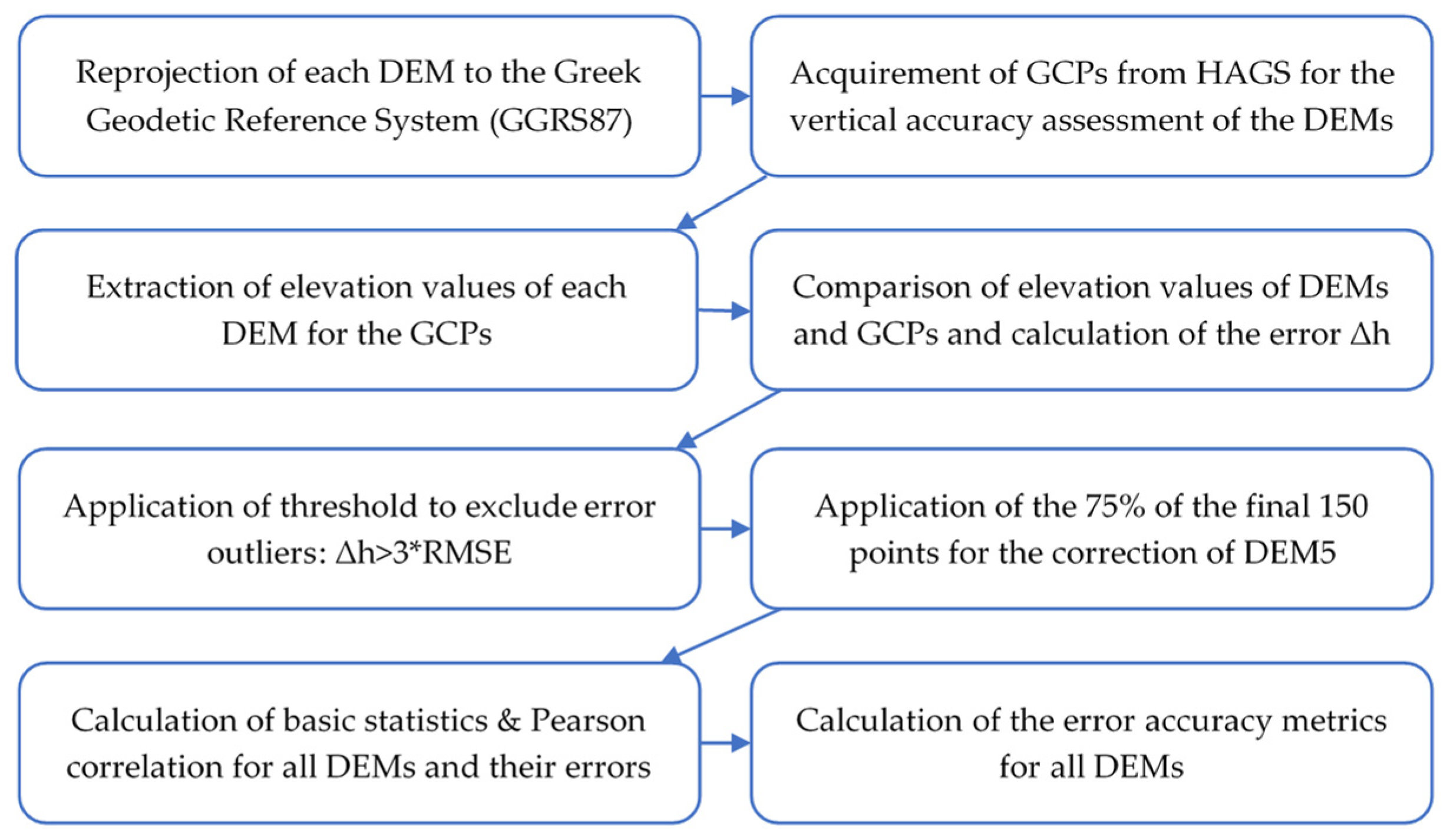
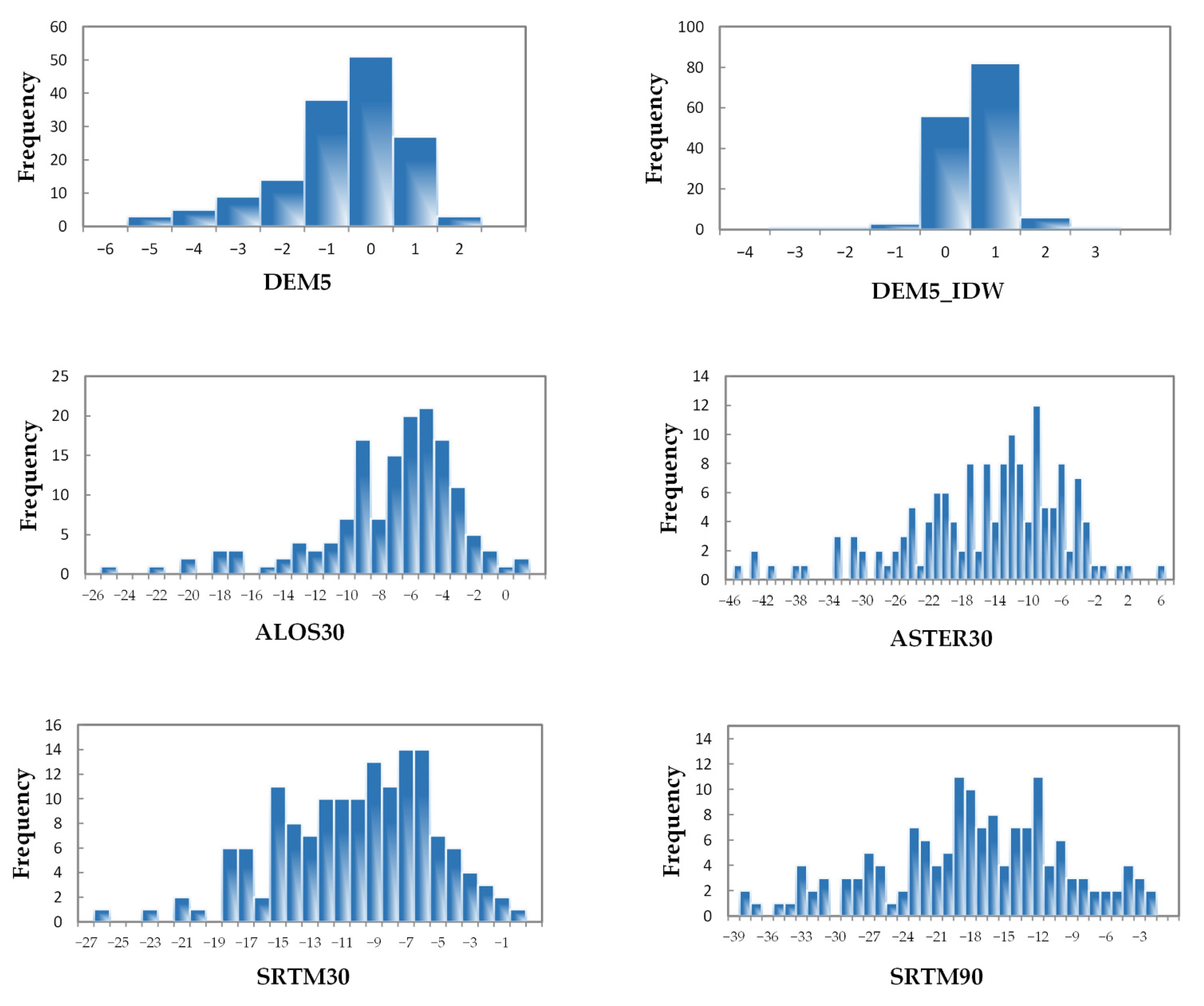
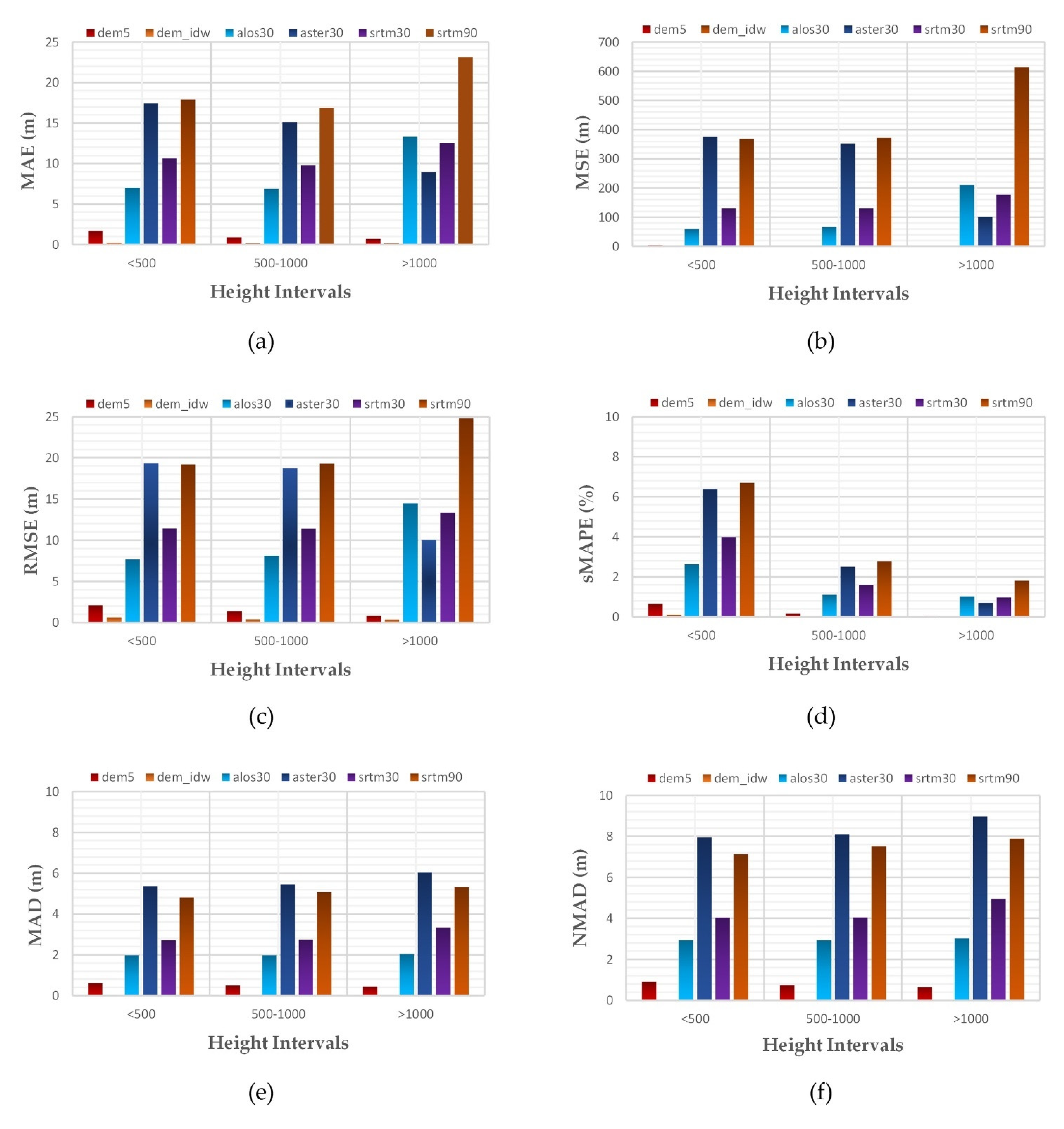
In this research, 6 DEM (2 DTM and 4 DSM) from different sources and with various resolutions, were acquired to evaluate their suitability for soil erosion modelling. The first section of this study contains the evaluation of the relative vertical accuracy of the examined DEM by comparing them to GCP. Initially, the error (Δh) was calculated by subtracting the altimetric value of each checkpoint from the corresponding value of each DEM. The basic statistics of the error, as well as more sufficient indices like MAE, MSE, RMSE, and sMAPE, were calculated too. These metrics showed that the DTM derived from the Hellenic Cadastre (DEM5) and the corrected one (DEM5_IDW) are performing better than the other DEM with RMSE values of 1.80 m and 0.54, respectively. Following this, ALOS30 and SRTM30 appear to have less satisfactory RMSE values equal to 8.95 m and 11.67 m, respectively, while ASTER30 (RMSE: 18.27 m) and SRTM90 (RMSE: 20.02 m) are underperforming with RMSE values of approximately 20 m. The calculated RMSE value of ALOS30 for the pilot area is also supported by the studies of Nikolakopoulos [33] and Stamatiou et al. [65] which reported RMSE values for the Greek territory equal to 8.58 m and 8.75 m, respectively. The RMSE value of ASTER30 was quite higher, almost double, the corresponding value that was estimated by other studies for the Greek territory, which reported an RMSE value equal to 10 m [68,69]. That is also the case for SRTM30, as reported RMSE values from other studies equal to 6.1 m [69] and 6.8 m [
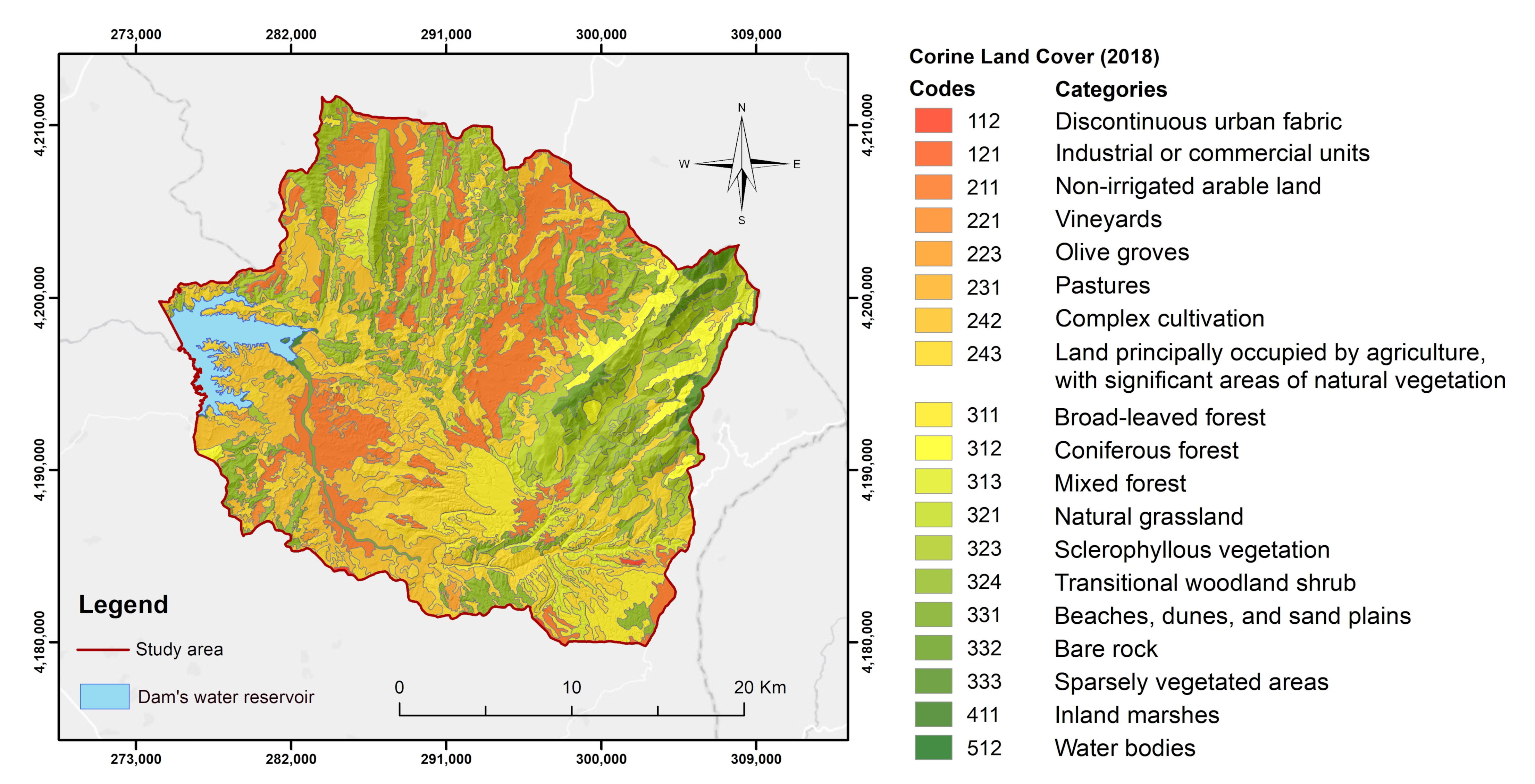
69] are almost half of the calculated one for the pilot area. The thorough eminence of the DEM5 and DEM5_IDW is also endorsed by the estimation of two more robust metrics, the MAD and NMAD. These metrics follow almost the same sequence from lowest to highest value as RMSE, with the exception that ASTER30 appears to have the highest MAD and NMAD values, followed by SRTM90. The underperformance of ASTER30 may be linked to the fact that the study area is mainly occupied by agriculture, which occurs in areas with relatively flat terrain where ASTER DEM shows lower vertical accuracy [68,73].
The comparison of DEM with different cell sizes provides essential information regarding the accuracy of their elevation data, while the comparison of the DEM derivative files such as slope is a more complicated process. The similarity of the statistics of the DEM elevation values is quite high even though they have different resolutions and sources, but in the case of a slope, the effect of the resolution is more evident. According to the work of Carrera-Hernandez, who examined the vertical accuracy of 8 DSMs from different sources in Mexico, it was shown that slope is the major factor that influences the error of DSMs among vegetation and aspect [78]. Zhou et al. analyzed the errors of slope and aspect with the used algorithms and the DEM properties and pointed out that even though DEM with high resolution have more details, the data error tends to increase, in contrast to the low-resolution DEM in which the data error has less influence while the error associated with algorithms increases, meaning that high-resolution DEM does not guarantee high accuracy for its deliverables [108]. The comparison of slopes for the evaluated DEM in the research area showed considerable variations. The DEM resolution has a major impact on the calculation of slope. The frequency of steeper slopes tends to increase in DEM with high resolution, as the DEM5 and DEM5_IDW with a 5 m resolution have the highest maximum and mean values, compared to the SRTM90 with a 90 m resolution, which shows the lowest maximum and mean values of all DEM.
DEM resolution and DEM source are very important parameters that influence the accuracy of soil erosion models [42,43]. Most of the time, the DEM have been used in soil erosion modelling studies without considering the examination of their adequacy regarding the accuracy and the quality of the source data which plays a significant role in the outcomes [30,45]. It is also important to consider the fact that both DTM and DSM data have been used in soil erosion modelling. By definition, a DTM refers to the bare ground surface, and it is considered to be the correct type of DEM for applications such as soil erosion simulations. The implementation of DSM data in soil erosion modelling is mainly due to the wide availability of freely acquired DSMs like those that were used in the current research. The fact that DSMs include the elevation of the canopy and man-made constructions can produce substantial errors in the calculations of the LS factor and, subsequently, soil erosion.
The effect of DEM in soil erosion modelling was examined by many researchers using the LISEM model (Limburg Soil Erosion Model) and DEM with different pixel sizes and concluded that large pixel sizes tend to cause a reduction in the estimations of soil loss, which is influenced primarily by the reduction of the DEM derived slope caused by the usage of DEM with large pixel size [42,113,114]. In the study of Chidi et al., the RUSLE model was applied using DEM with varying resolutions from 5 cm to 10 m in the Middle Hill area in Nepal [115]. This research pointed out that by increasing the pixel size in DEM, the expected slope gradient will decrease, influencing the LS factor and the estimated soil loss, which also decreases with the increase of DEM pixel size [115]. The current statement that LS factor values decrease with coarser DEM is following the studies of [36,37,39,115] and is in contrast to the study of Shan et al. [38].
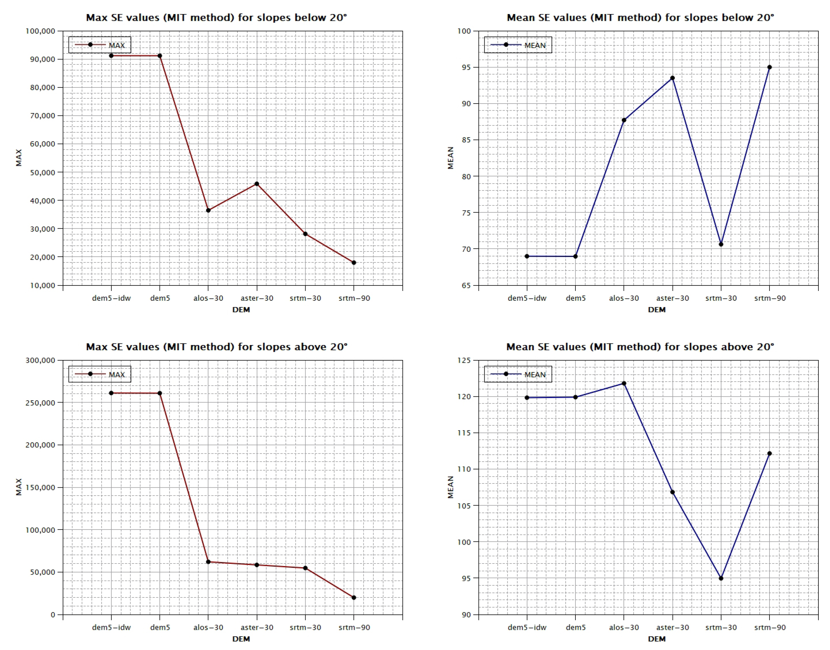
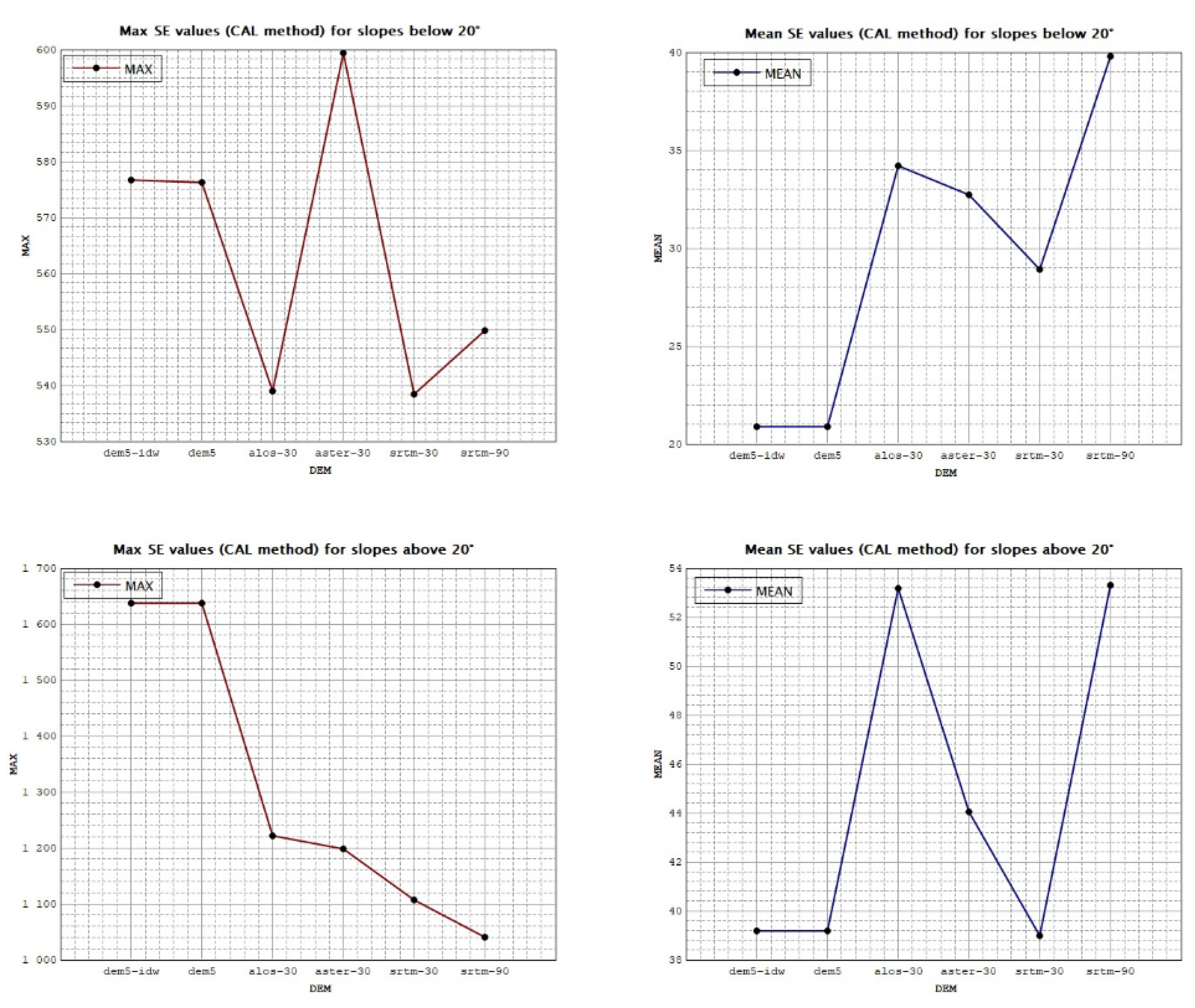
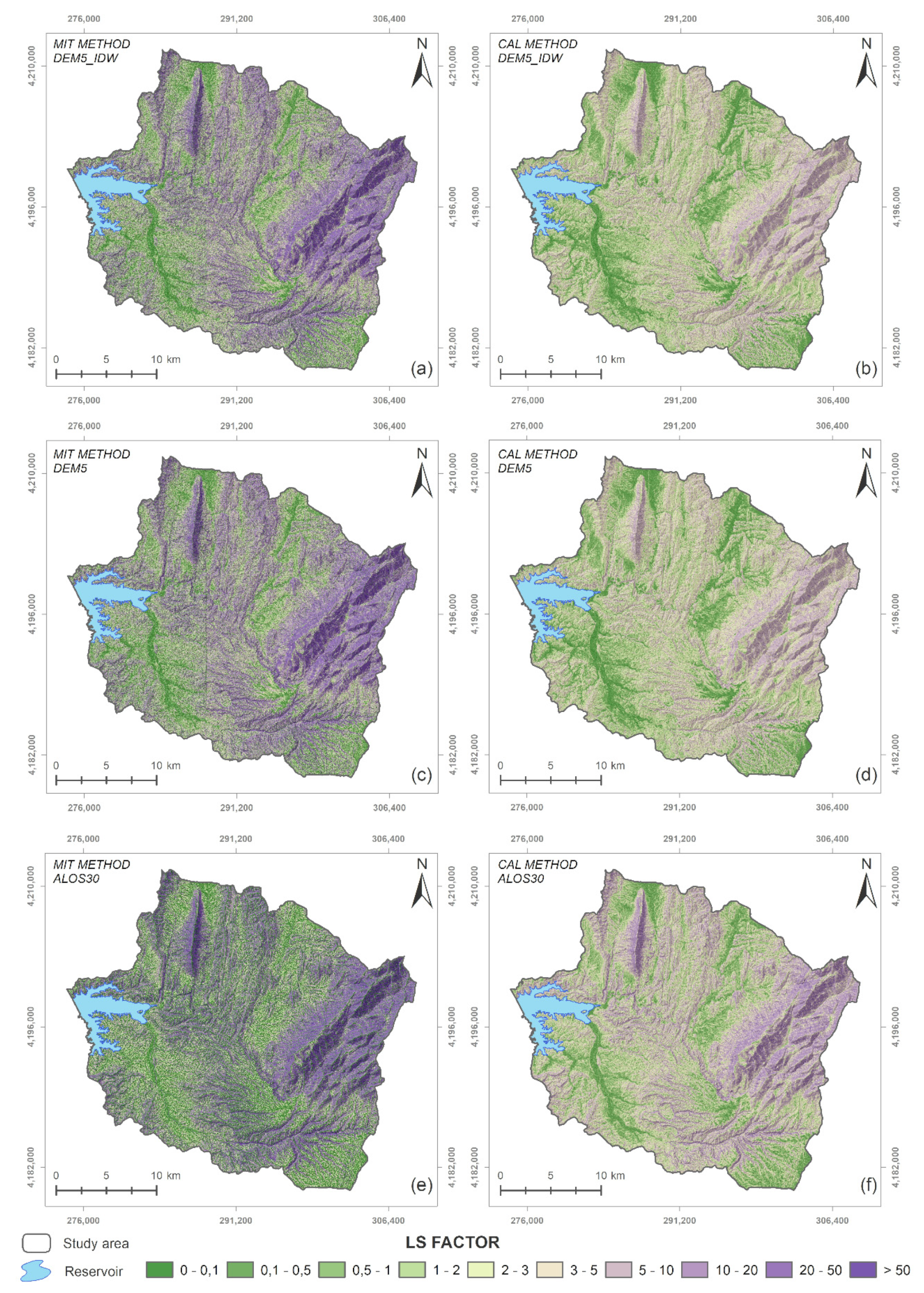
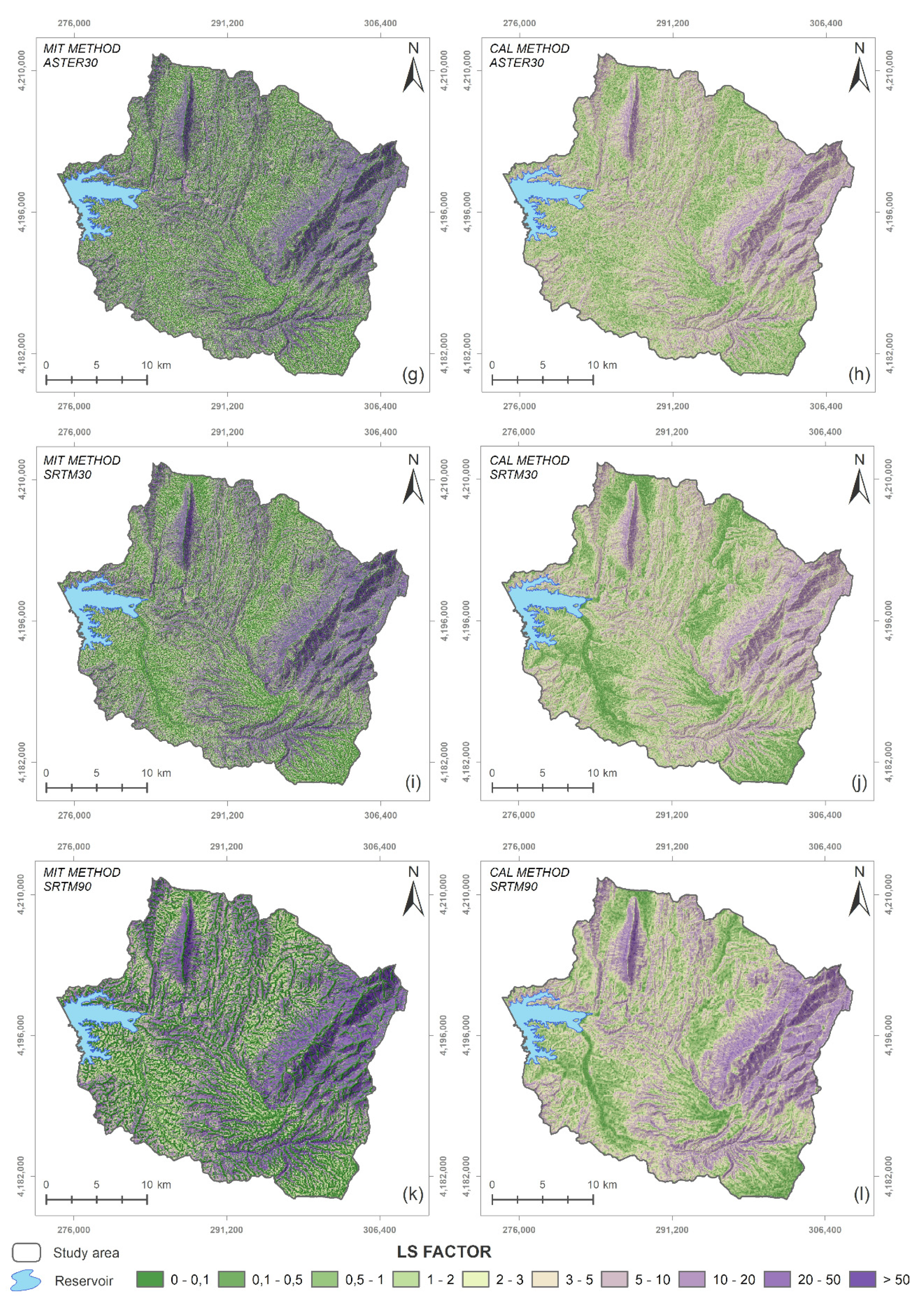
The high LS values of the MIT method are related to the fact that this LS equation is an integral part of the USPED model (Unit Stream Power—based Erosion Deposition), and therefore should be interpreted in the context of this model. It should also be considered that the USPED model [47] allows the estimation not only of the net erosion but also determines the deposition in a basin, unlike the RUSLE model [116]. According to Karásek et al., the LS factor calculated with this method is characterized by a line structure of pixel cells in which the LS factor values are increasing accordingly to the direction of overland flow downstream of the slope [
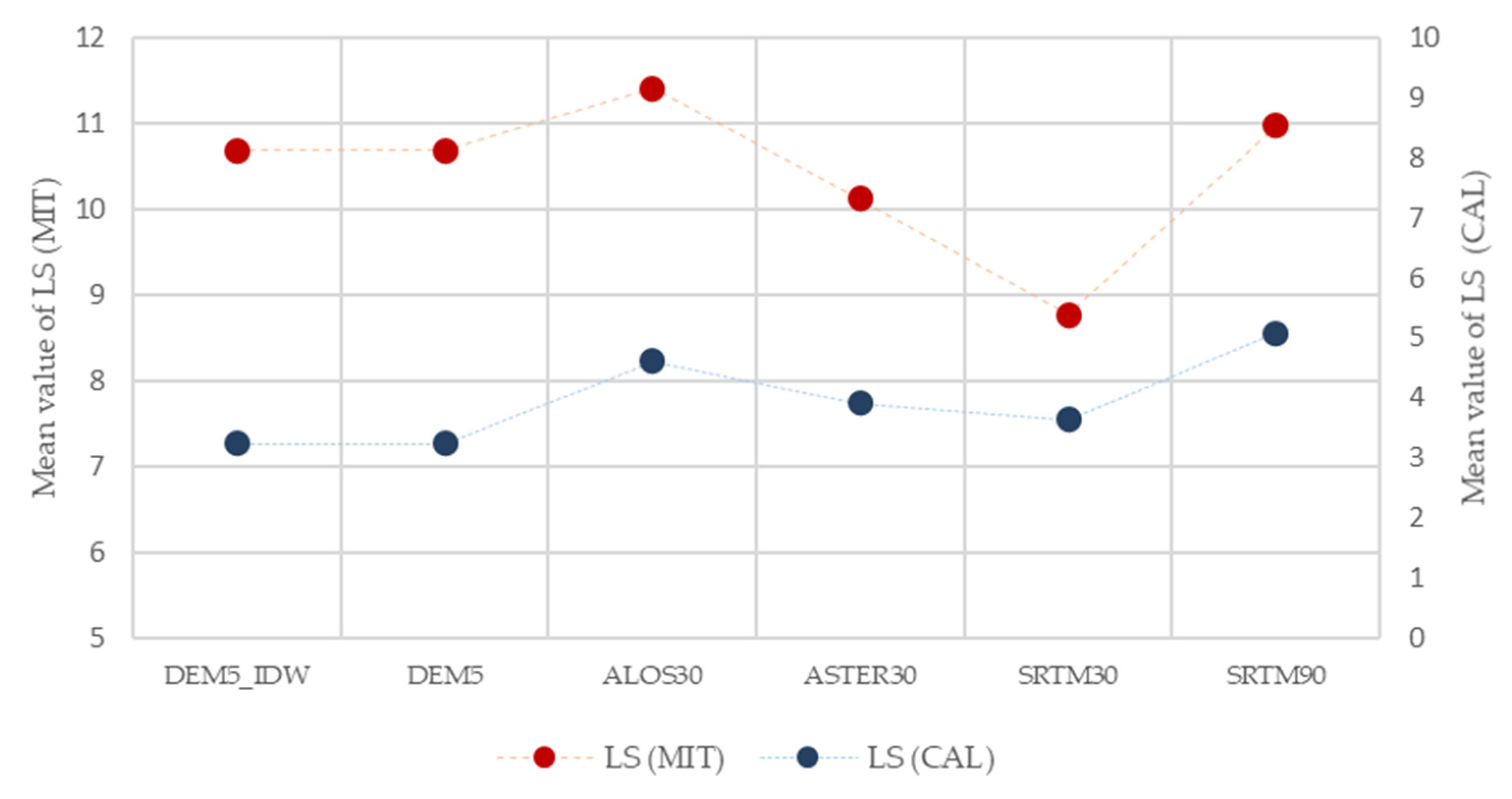
117]. This leads to a sharp transition between the high and low LS values, which are associated with the use of the flow accumulation in this equation and result in quite high mean LS values. An important difference between these approaches is that the MIT method uses the upstream contribution area or the specific catchment area (A) whereas the CAL method uses the slope length (λ) for the calculation of the slope length or L factor. More specifically, in the case of the CAL method, a threshold of 305 m was considered in the slope length calculations. Regarding the slope steepness, or S factor, a threshold slope value of 9% was taken into consideration. It is also noted that the calculated mean LS factors from the MIT and the CAL method were compared with the estimated mean LS value that was calculated by the European Soil Data Centre (ESDAC), which developed a pan-European high-resolution soil erosion assessment. This comparison was conducted in the circumstance that there are no field measurements available for the evaluation of the LS factor. This LS factor assessment showed that the LS values calculated from the CAL method, with a range of 3.24 (from DEM5_IDW) to 5.08 (from SRT90), were very close to the corresponding value from ESDAC, which is equal to 3.31, while the corresponding values from the MIT method are significantly higher, ranging from 8.77 (from SRTM30) to 11.41 (from ALOS30). This indicates that the CAL method performs better in the pilot area.

6. Conclusions

The objective of this research is to examine the connection between DEM and the LS factor, which is one of the most significant parameters of the RUSLE model, to estimate soil erosion annual rates. Due to the dense morphology of the research area and its susceptibility to soil erosion, the examination of the quality of DEM has proved to be an important issue.
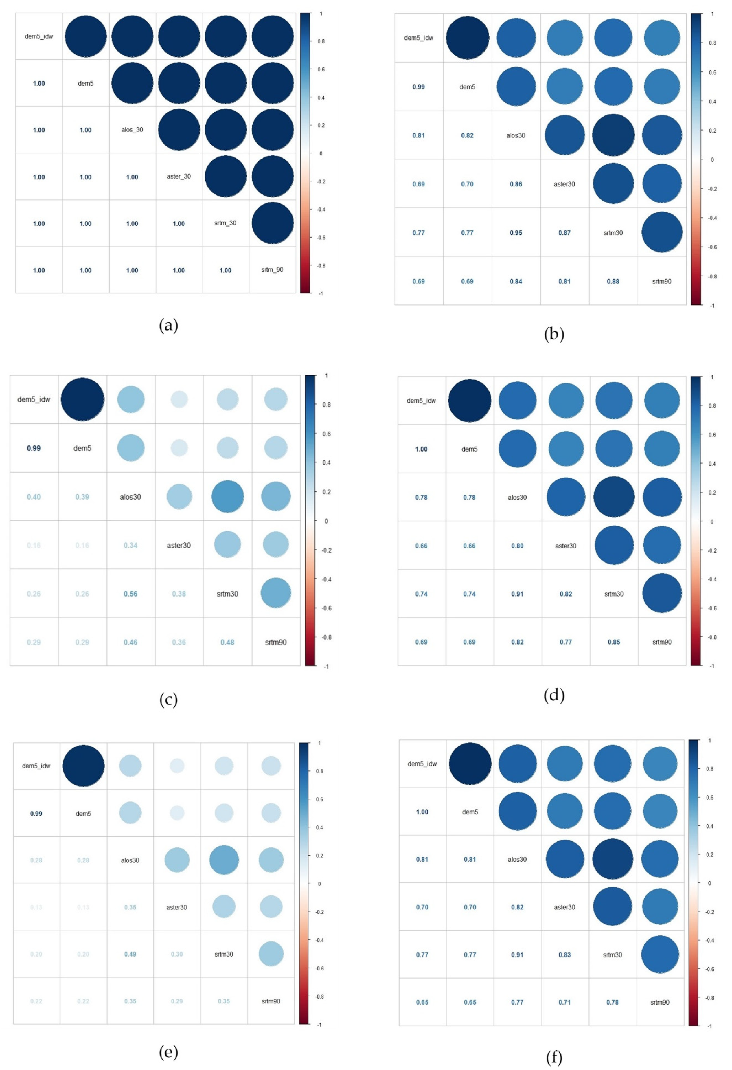
Regarding the DEM analysis, which was performed in this study, the elevation data showed a satisfactory similarity based on the high values of the calculated Pearson correlation index. Based on the statistical assessment, the DEM5 and the corrected DEM5_IDW were found to be better compared with the other DEM, followed by ALOS30, SRTM30, ASTER30, and SRTM90, and the calculated error increased with the increase of the elevation (>1000 m) for all DEM. The comparison of the slopes from each of the 6 examined DEM showed a greater discrepancy, mainly because of the different DEM cell sizes and their types, as both DTMs and DSMs were acquired for this research.
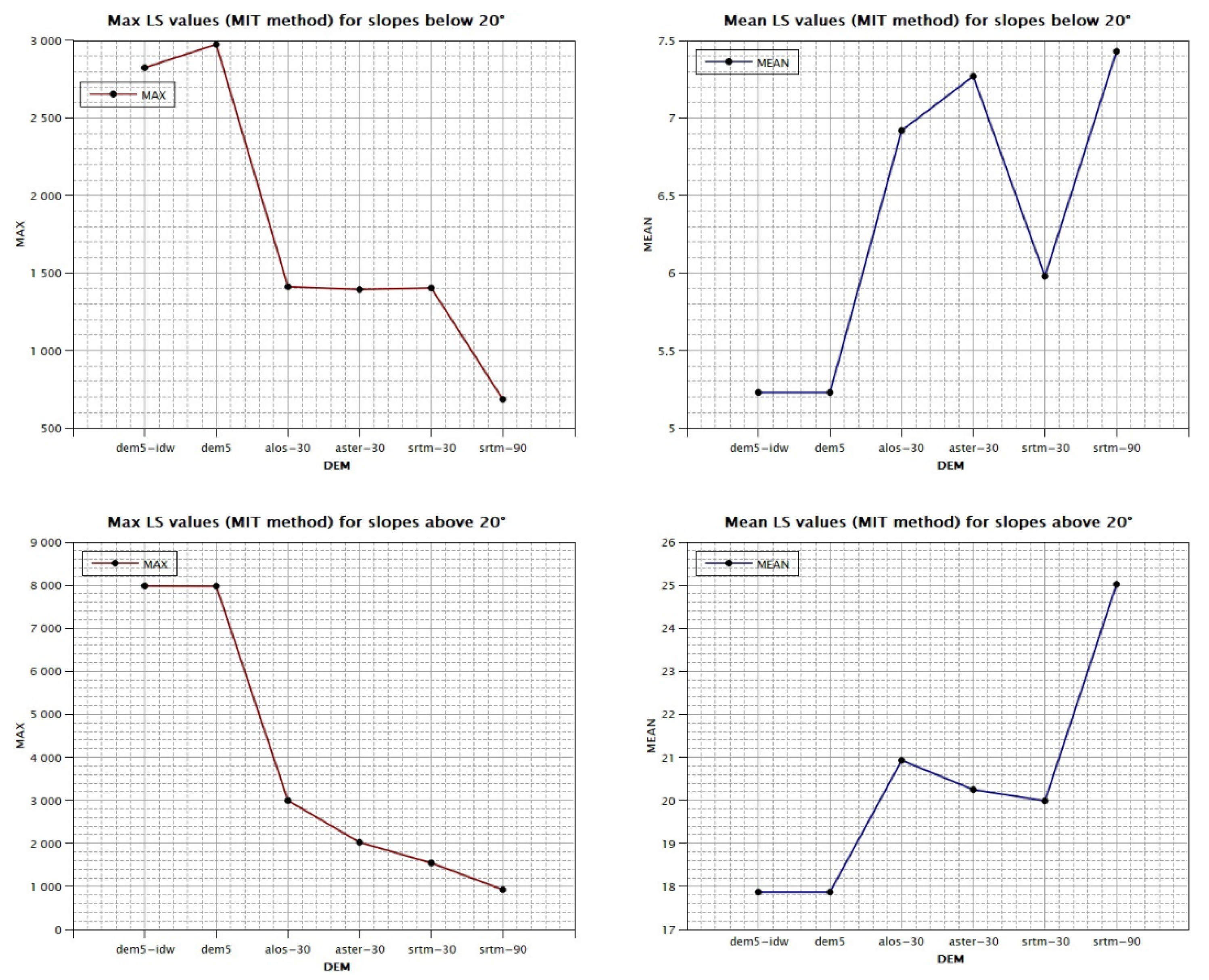
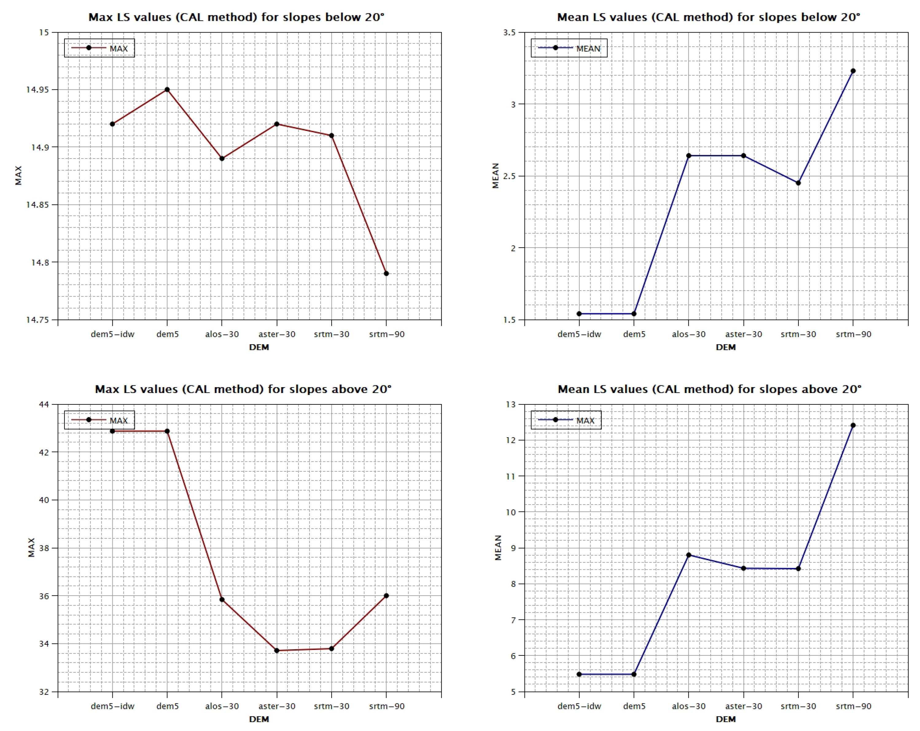
The computation of the LS factor was performed with the application of two different methods. The first method proposed by Mitasova et al. [46,47] showed much higher LS values than the second one proposed by the CALSITE method. Increasing the DEM grid size, the calculated LS mean values were increased in the case of the CAL method, but for the MIT method, the results did not follow a specific sequence. Regarding max LS values, the DEM with the 5 m resolution showed the highest value in both cases. The lowest value was calculated from the SRTM90 with the MIT method, in contrast to the CAL method, as the SRTM90 had the second highest value. The evaluation of the correlation using the Pearson coefficient showed that the LS values calculated with the CAL method for each DEM have a higher similarity with each other than the LS values for each DEM from the MIT method, which showed a great divergence. Both of the LS factor computation methods presented significantly higher values for slopes that exceed 20° for all the examined DEM.
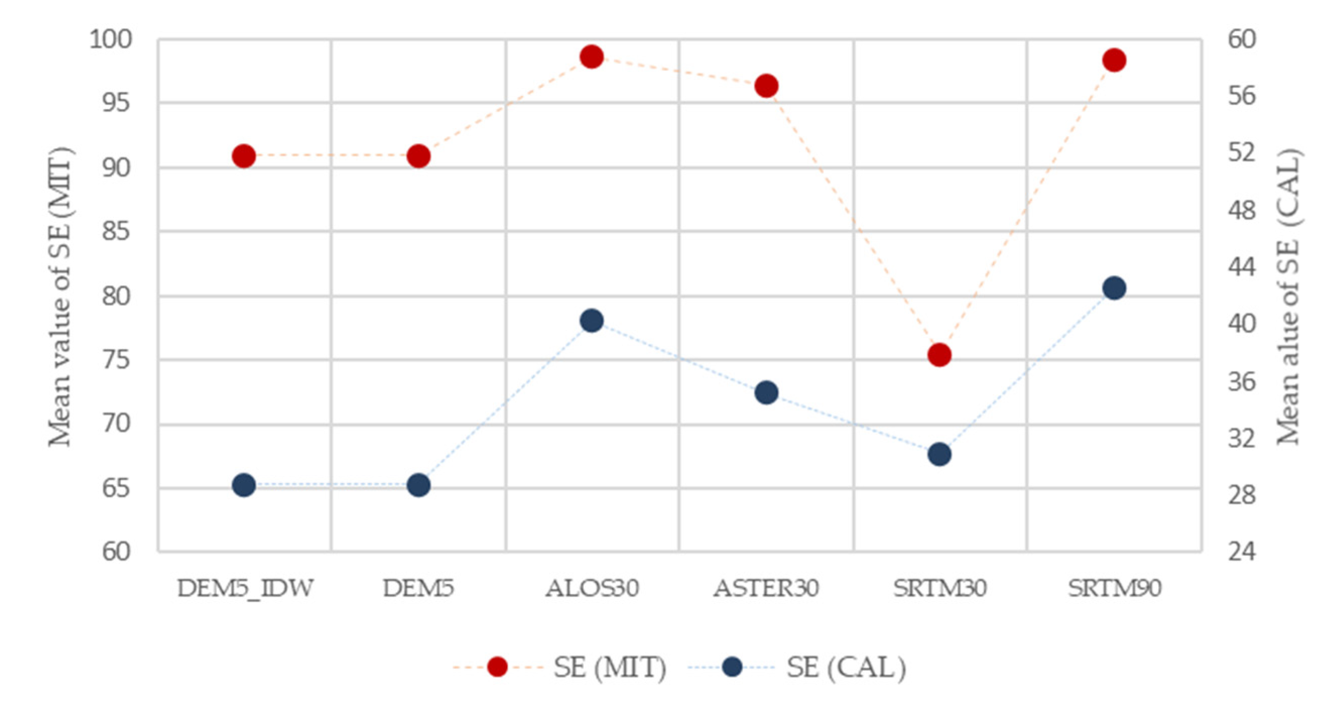
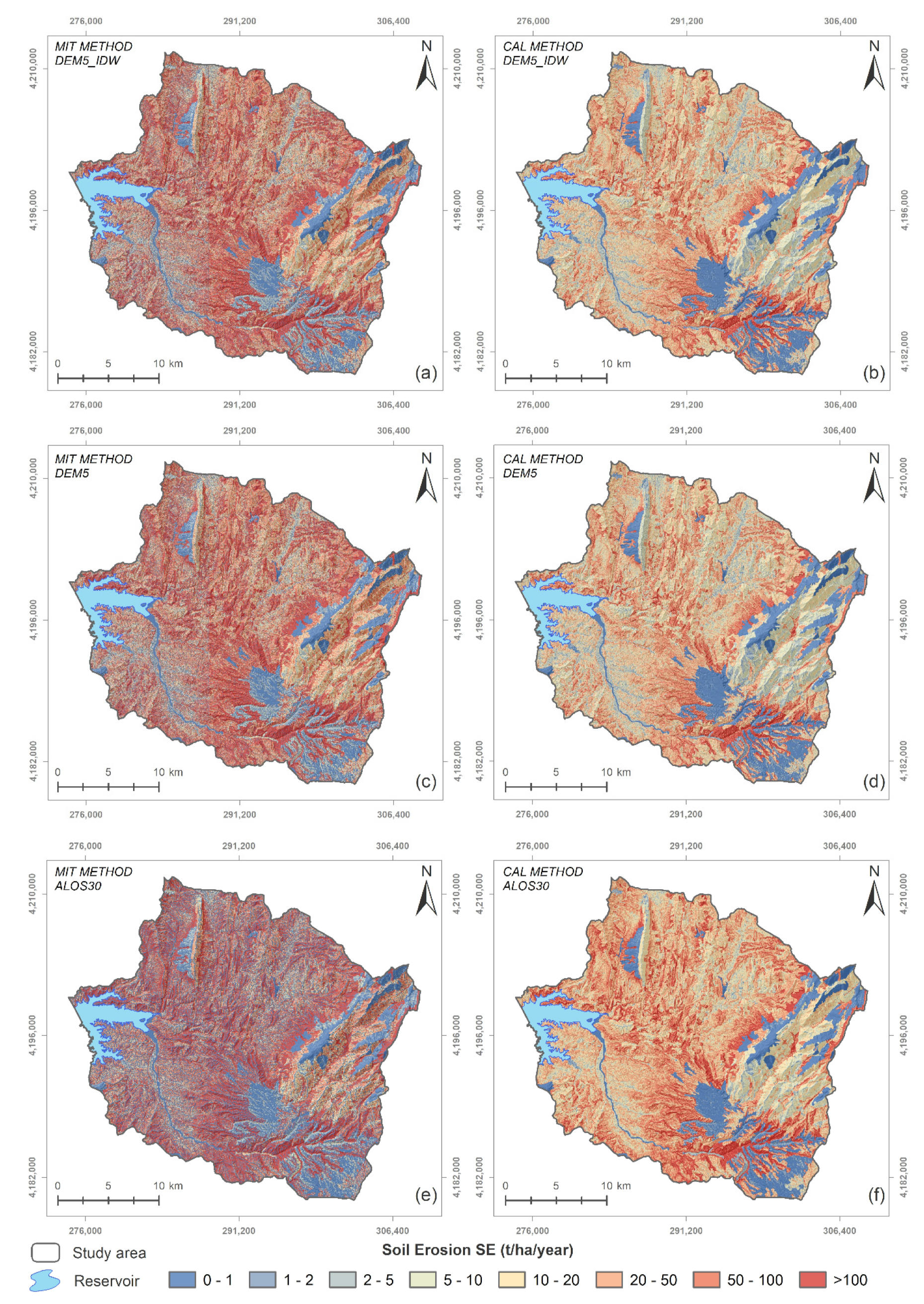
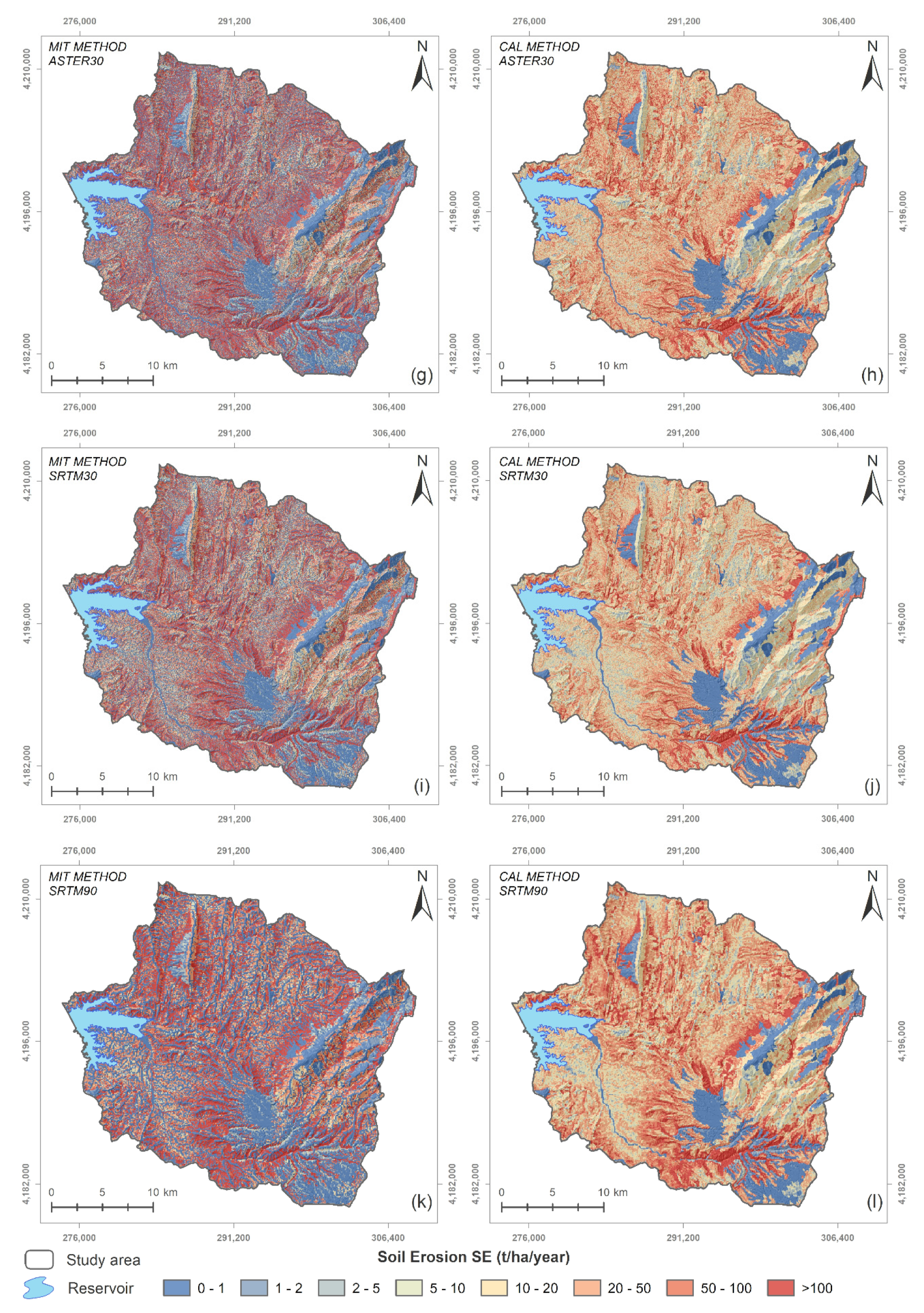
As for soil loss, the mean SE annual rates calculated for each DEM using the CAL method are significantly lower than the relevant SE values calculated using the MIT method, following the same pattern as the calculated LS factor. The Pearson correlation index showed greater similarity in SE values calculated with the LS factor from the CAL method compared to the MIT method, and in both cases, SE values estimated for slopes above 20° were substantially increased.
The different results derived from various studies regarding the LS factor are related to the different approaches in each applied methodology, the special characteristics related to the landscape for the area of interest, the different sources of examined DEM, and the different LS factor equations. The comparison of the LS values calculated with the two examined approaches and with the use of different DEM data with various resolutions and from diverse sources does not change consistently with the increase of DEM grid size and accuracy. This is also supported by the study of Fijałkowska, which stated that the relationship between DEM resolution and LS factor is indeed complex because the LS factor from one DEM can produce high values for the same area where the LS factor from another DEM calculates low values [45].
The use of adequate data is essential for soil erosion modelling. In particular, the accuracy of topographic data like DEM plays a vital role in the identification of soil erosion high-risk areas. The precise detection of soil erosion-prone areas is very important for protection measurement planning. The sustainability of the examined areas defines the types of applications that need to be fulfilled. Nature-based solutions are considered to be proper, mainly for areas occupied by a high percentage of agricultural land, as their benefits are long-term and cost-efficient [118].
In conclusion, this research highlighted the importance of evaluating the primary topographic data and the different approaches to LS factor calculation before continuing with the assessment of soil erosion modelling, especially in areas with diverse landscape. It seems that the use of an LS equation that imports thresholds in its formula, such as the CALSITE method, helps to avoid overestimation in soil loss calculations. The next step requires field measurements to evaluate and validate the different data and methods used regarding the LS factor and to define which method is the most appropriate for the corresponding area of interest. Towards this aspect, different methodologies and models like WATEM/SEDEM and the InVEST SDR model could be acquired.

Author Contributions

Conceptualization, M.M. and N.D.; methodology, M.M. and N.D.; validation, N.D. and K.N.; formal analysis, M.M. and V.B.; investigation, M.M. and N.D.; resources, N.D.; data curation, M.M., N.D., K.N. and V.B.; writing—original draft preparation, M.M.; writing—review and editing, M.M., N.D. and K.N.; visualization, M.M. and N.D.; supervision, N.D.; project administration, N.D.; funding acquisition, N.D. All authors have read and agreed to the published version of the manuscript.

Funding

This research was financially supported by the «Andreas Mentzelopoulos Foundation».

Institutional Review Board Statement

Not applicable.

Informed Consent Statement

Not applicable.

Data Availability Statement

Data are available from the authors upon request.

Acknowledgments

The authors acknowledge the support of «Andreas Mentzelopoulos Foundation».

Conflicts of Interest

The authors declare no conflict of interest. The funders had no role in the design of the study; in the collection, analyses, or interpretation of data; in the writing of the manuscript, or in the decision to publish the results.

Appendix A

Figure A1. Histograms of the error (Δh) for all the DEM data (DEM5, DEM5_IDW, ALOS30, ASTER30, SRTM30 and SRTM90) showing the non-normality of the error distribution.
Land 11 01592 g0a1
Figure A2. Histograms of the statistical coefficients of the height intervals <500, 500–1000, >1000 for each DEM (a) MAE, (b) MSE, (c) RMSE, (d) sMAPE, (e) MAD, (f) NMAD.
Land 11 01592 g0a2
Figure A3. Pearson correlation charts of (a) DEM, (b) Slopes, (c) LS from MIT method, (d) LS from CAL method, (e) SE from MIT method and (f) SE from CAL method.
Land 11 01592 g0a3

Appendix B

Figure A4. Maps of LS factor calculated with the MIT method applied on DEM5_IDW (a), DEM5 (c), and ALOS30 (e) as well as the CAL method based on DEM5_IDW (b), DEM5 (d), and ALOS30 (f).
Land 11 01592 g0a4
Figure A5. Maps of LS factor calculated with the MIT method applied on ASTER30 (g), SRTM30 (i), and SRTM90 (k) as well as the CAL method based on ASTER30 (h), SRTM30 (j), and SRTM90 (l).
Land 11 01592 g0a5
Figure A6. Maps of soil erosion annual rates (SE) calculated with the LS factor computed with the MIT method applied on DEM5_IDW (a), DEM5 (c), and ALOS30 (e) as well as the CAL method applied on DEM5_IDW (b), DEM5 (d), and ALOS30 (f).
Land 11 01592 g0a6
Figure A7. Maps of soil erosion annual rates (SE) calculated with the LS factor computed with the MIT method applied on ASTER30 (g), SRTM30 (i), SRTM90 (k) as well as the CAL method applied on ASTER30 (h), SRTM30 (j), and SRTM90 (l).
Land 11 01592 g0a7

References

  1. Lutgens, F.K.; Tarbuck, E.J. Essentials of Geology, 11th ed.; Prentice Hall: Boston, UK, 2012; ISBN 9780321714725. [Google Scholar]
  2. Wakatsuki, T.; Rasyidin, A. Rates of Weathering and Soil Formation. Geoderma 1992, 52, 251–263. [Google Scholar] [CrossRef]
  3. Commission, E. EU Soil Strategy for 2030 Reaping the Benefits of Healthy Soils for People, Food, Nature and Climate. 2021. Available online: https://environment.ec.europa.eu/strategy/soil-strategy_en (accessed on 25 June 2022).
  4. Veerman, C.; Correia, T.P.; Bastioli, C.; Biro, B.; Bouma, J.; Cienciala, E.; Emmett, B.; Frison, E.A.; Grand, A.; Filchev, L.H. Caring for Soil Is Caring for Life: Ensure 75% of Soils Are Healthy by 2030 for Healthy Food, People, Nature and Climate: Interim Report of the Mission Board for Soil Health and Food: Study. 2020. Available online: https://data.europa.eu/doi/10.2777/821504 (accessed on 24 March 2022).
  5. Panagos, P.; Borrelli, P.; Poesen, J.; Ballabio, C.; Lugato, E.; Meusburger, K.; Montanarella, L.; Alewell, C. The New Assessment of Soil Loss by Water Erosion in Europe. Environ. Sci. Policy 2015, 54, 438–447. [Google Scholar] [CrossRef]
  6. Van der Knijff, J.M.; Jones, R.J.A.; Montanarella, L. Soil Erosion Risk: Assessment in Europe 2000. Available online: https://esdac.jrc.ec.europa.eu/content/soil-erosion-risk-assessment-europe (accessed on 20 February 2022).
  7. Brini, I.; Alexakis, D.D.; Kalaitzidis, C. Linking Soil Erosion Modeling to Landscape Patterns and Geomorphometry: An Application in Crete, Greece. Appl. Sci. 2021, 11, 5684. [Google Scholar] [CrossRef]
  8. Panagos, P.; Ballabio, C.; Poesen, J.; Lugato, E.; Scarpa, S.; Montanarella, L.; Borrelli, P. A Soil Erosion Indicator for Supporting Agricultural, Environmental and Climate Policies in the European Union. Remote Sens. 2020, 12, 1365. [Google Scholar] [CrossRef]
  9. Cerdà, A.; Franch-Pardo, I.; Novara, A.; Sannigrahi, S.; Rodrigo-Comino, J. Examining the Effectiveness of Catch Crops as a Nature-Based Solution to Mitigate Surface Soil and Water Losses as an Environmental Regional Concern. Earth Syst. Environ. 2022, 6, 29–44. [Google Scholar] [CrossRef]
  10. Nearing, M.A.; Lane, L.J.; Lopes, V.L. Modeling Soil Erosion. In Soil Erosion Research Methods; Routledge: New York, NY, USA, 1994; pp. 127–158. ISBN 0203739353. [Google Scholar]
  11. Batista, P.V.G.; Davies, J.; Silva, M.L.N.; Quinton, J.N. On the Evaluation of Soil Erosion Models: Are We Doing Enough? Earth-Sci. Rev. 2019, 197, 102898. [Google Scholar] [CrossRef]
  12. Kourgialas, N.N.; Koubouris, G.C.; Karatzas, G.P.; Metzidakis, I. Assessing Water Erosion in Mediterranean Tree Crops Using GIS Techniques and Field Measurements: The Effect of Climate Change. Nat. Hazards 2016, 83, 65–81. [Google Scholar] [CrossRef]
  13. Cerdà, A.; Novara, A.; Moradi, E. Long-Term Non-Sustainable Soil Erosion Rates and Soil Compaction in Drip-Irrigated Citrus Plantation in Eastern Iberian Peninsula. Sci. Total Environ. 2021, 787, 147549. [Google Scholar] [CrossRef]
  14. Zingg, A.W. Degree and Length of Land Slope as It Affects Soil Loss in Run-Off. Agric. Engng. 1940, 21, 59–64. [Google Scholar]
  15. Morgan, R.P.C. Soil Erosion and Conservation; Wiley: New York, NY, USA, 2005; ISBN 9781405117814. [Google Scholar]
  16. Musgrave, G.W. The Quantitative Evaluation of Factors in Water Erosion: A First Approximation. J. Soil Water Conserv. 1947, 2, 133–138. [Google Scholar]
  17. Smith, D.D. Factors Affecting Rainfall Erosion and Their Evaluation. Int. Assoc. Sci. Hydrol. Publ. 1958, 43, 97–107. [Google Scholar]
  18. Wischmeier, W.; Smith, D. Predicting Rainfall Erosion Losses—A Guide To Conservation Planning. Agric. Handb. 1978, 537, 62. [Google Scholar]
  19. Renard, K.G.; Foster, R.G.; Weesies, G.A.; Porter, J.P.C. RUSLE: Revised Universal Soil Loss Equation. J. Soil Water Conserv. 1991, 46, 30–33. [Google Scholar]
  20. Williams, J.R.; Berndt, H.D. Sediment Yield Prediction Based on Watershed Hydrology. Trans. ASAE 1977, 20, 1100–1104. [Google Scholar] [CrossRef]
  21. Morgan, R.P.C.; Quinton, J.N.; Smith, R.E.; Govers, G.; Poesen, J.W.A.; Auerswald, K.; Chisci, G.; Torri, D.; Styczen, M.E. The European Soil Erosion Model (EUROSEM): A Dynamic Approach for Predicting Sediment Transport from Fields and Small Catchments. Earth Surf. Process. Landf. J. Br. Geomorphol. Gr. 1998, 23, 527–544. [Google Scholar] [CrossRef]
  22. Kirkby, M.J.; Irvine, B.J.; Jones, R.J.A.; Govers, G.; Team, P. The PESERA Coarse Scale Erosion Model for Europe. I.–Model Rationale and Implementation. Eur. J. Soil Sci. 2008, 59, 1293–1306. [Google Scholar] [CrossRef]
  23. Efthimiou, N.; Psomiadis, E.; Panagos, P. Fire Severity and Soil Erosion Susceptibility Mapping Using Multi-Temporal Earth Observation Data: The Case of Mati Fatal Wildfire in Eastern Attica, Greece. Catena 2020, 187, 104320. [Google Scholar] [CrossRef]
  24. Depountis, N.; Michalopoulou, M.; Kavoura, K.; Nikolakopoulos, K.; Sabatakakis, N. Estimating Soil Erosion Rate Changes in Areas Affected by Wildfires. ISPRS Int. J. Geo-Inf. 2020, 9, 562. [Google Scholar] [CrossRef]
  25. Polykretis, C.; Alexakis, D.D.; Grillakis, M.G.; Manoudakis, S. Assessment of Intra-Annual and Inter-Annual Variabilities of Soil Erosion in Crete Island (Greece) by Incorporating the Dynamic “Nature” of R and C-Factors in RUSLE Modeling. Remote Sens. 2020, 12, 2439. [Google Scholar] [CrossRef]
  26. Xanthakis, M.; Pavlopoulos, K.; Kapsimalis, V.; Apostolopoulos, G.; Xanthopoulos, G.; Stefanidis, P.; Evelpidou, N. Prediction of Soil Loss in a Reservoir Watershed Using an Erosion Model and Modern Technological Tools: A Case Study of Marathon Lake, Attica in Greece. Environ. Sci. Proc. 2020, 2, 63. [Google Scholar]
  27. Stefanidis, S.; Alexandridis, V.; Chatzichristaki, C.; Stefanidis, P. Assessing Soil Loss by Water Erosion in a Typical Mediterranean Ecosystem of Northern Greece under Current and Future Rainfall Erosivity. Water 2021, 13, 2002. [Google Scholar] [CrossRef]
  28. Tselka, I.; Krassakis, P.; Rentzelos, A.; Koukouzas, N.; Parcharidis, I. Assessing Post-Fire Effects on Soil Loss Combining Burn Severity and Advanced Erosion Modeling in Malesina, Central Greece. Remote Sens. 2021, 13, 5160. [Google Scholar] [CrossRef]
  29. Stefanidis, S.; Alexandridis, V.; Ghosal, K. Assessment of Water-Induced Soil Erosion as a Threat to Natura 2000 Protected Areas in Crete Island, Greece. Sustainability 2022, 14, 2738. [Google Scholar] [CrossRef]
  30. Datta, P.S.; Schack-Kirchner, H. Erosion Relevant Topographical Parameters Derived from Different DEMs—A Comparative Study from the Indian Lesser Himalayas. Remote Sens. 2010, 2, 1941–1961. [Google Scholar] [CrossRef]
  31. Höhle, J.; Potuckova, M. Assessment of the Quality of Digital Terrain Models; European Spatial Data Research: Frankfurt, Germany, 2011; ISBN 9789051797877. [Google Scholar]
  32. Polidori, L.; El Hage, M. Digital Elevation Model Quality Assessment Methods: A Critical Review. Remote Sens. 2020, 12, 3522. [Google Scholar] [CrossRef]
  33. Nikolakopoulos, K.G. Accuracy Assessment of ALOS AW3D30 DSM and Comparison to ALOS PRISM DSM Created with Classical Photogrammetric Techniques. Eur. J. Remote Sens. 2020, 53, 39–52. [Google Scholar] [CrossRef]
  34. Panagos, P.; Borrelli, P.; Meusburger, K. A New European Slope Length and Steepness Factor (LS-Factor) for Modeling Soil Erosion by Water. Geosciences 2015, 5, 117–126. [Google Scholar] [CrossRef]
  35. Efthimiou, N.; Lykoudi, E.; Psomiadis, E. Inherent Relationship of the USLE, RUSLE Topographic Factor Algorithms and Its Impact on Soil Erosion Modelling. Hydrol. Sci. J. 2020, 65, 1879–1893. [Google Scholar] [CrossRef]
  36. Fu, S.; Cao, L.; Liu, B.; Wu, Z.; Savabi, M.R. Effects of DEM Grid Size on Predicting Soil Loss from Small Watersheds in China. Environ. Earth Sci. 2015, 73, 2141–2151. [Google Scholar] [CrossRef]
  37. Mondal, A.; Khare, D.; Kundu, S.; Mukherjee, S.; Mukhopadhyay, A.; Mondal, S. Uncertainty of Soil Erosion Modelling Using Open Source High Resolution and Aggregated DEMs. Geosci. Front. 2017, 8, 425–436. [Google Scholar] [CrossRef]
  38. Shan, L.; Yang, X.; Zhu, Q. Effects of DEM Resolutions on LS and Hillslope Erosion Estimation in a Burnt Landscape. Soil Res. 2019, 57, 797–804. [Google Scholar] [CrossRef]
  39. Lu, S.; Liu, B.; Hu, Y.; Fu, S.; Cao, Q.; Shi, Y.; Huang, T. Soil Erosion Topographic Factor (LS): Accuracy Calculated from Different Data Sources. Catena 2020, 187, 104334. [Google Scholar] [CrossRef]
  40. Wang, C.; Shan, L.; Liu, X.; Yang, Q.; Cruse, R.M.; Liu, B.; Li, R.; Zhang, H.; Pang, G. Impacts of Horizontal Resolution and Downscaling on the USLE LS Factor for Different Terrains. Int. Soil Water Conserv. Res. 2020, 8, 363–372. [Google Scholar] [CrossRef]
  41. Kruk, E.; Klapa, P.; Ryczek, M.; Ostrowski, K. Influence of Dem Elaboration Methods on the Usle Model Topographical Factor Parameter on Steep Slopes. Remote Sens. 2020, 12, 3540. [Google Scholar] [CrossRef]
  42. Azizian, A.; Koohi, S. The Effects of Applying Different DEM Resolutions, DEM Sources and Flow Tracing Algorithms on LS Factor and Sediment Yield Estimation Using USLE in Barajin River Basin (BRB), Iran. Paddy Water Environ. 2021, 19, 453–468. [Google Scholar] [CrossRef]
  43. Pandey, A.; Gautam, A.K.; Chowdary, V.M.; Jha, C.S.; Cerdà, A. Uncertainty Assessment in Soil Erosion Modelling Using RUSLE, Multisource and Multiresolution DEMs. J. Indian Soc. Remote Sens. 2021, 49, 1689–1707. [Google Scholar] [CrossRef]
  44. Kumar, N.; Singh, S.K. Soil Erosion Assessment Using Earth Observation Data in a Trans-Boundary River Basin. Nat. Hazards 2021, 107, 1–34. [Google Scholar] [CrossRef]
  45. Fijałkowska, A. Analysis of the Influence of DTM Source Data on the LS Factors of the Soil Water Erosion Model Values with the Use of GIS Technology. Remote Sens. 2021, 13, 678. [Google Scholar] [CrossRef]
  46. Mitasova, H.; Mitas, L. Multiscale Soil Erosion Simulations for Land Use Management. In Landscape Erosion and Evolution Modeling; Springer: Berlin/Heidelberg, Germany, 2001; pp. 321–347. [Google Scholar]
  47. Mitasova, H.; Hofierka, J.; Zlocha, M.; Iverson, L. Modelling Topographic Potential for Erosion and Deposition Using GIS. Int. J. Geogr. Inf. Sci. 1996, 10, 629–641. [Google Scholar] [CrossRef]
  48. Bradbury, P.; Lea, N.; Bolton, P. Estimating Catchment Sediment Yield: Development of the GIS-Based CALSITE Model. HR Wallingford. 1993. Available online: https://eprints.hrwallingford.com/330/ (accessed on 25 January 2022).
  49. Bolton, P.; Bradbury, P.A.; Lawrence, P.; Atkinson, E. CALSITE Version 3.1 Calibrated Simulation of Transported Erosion. In User Manual; HR Wallingford Ltd.: Wallingford, UK, 1995. [Google Scholar]
  50. Depountis, N.; Maria, V.; Kavoura, K.; Sabatakakis, N. Soil Erosion Prediction at the Water Reservoir’s Basin of Pineios Dam, Western Greece, Using the Revised Universal Soil Loss Equation (RUSLE) and GIS. WSEAS Trans. Environ. Dev. 2018, 14, 457–463. [Google Scholar]
  51. The CORINE Land Cover (CLC 2018) Inventory. Available online: https://land.copernicus.eu/pan-european/corine-land-cover/clc2018?tab=download (accessed on 10 November 2021).
  52. Lainas, S.; Depountis, N.; Sabatakakis, N. Preliminary Forecasting of Rainfall-Induced Shallow Landslides in the Wildfire Burned Areas of Western Greece. Land 2021, 10, 877. [Google Scholar] [CrossRef]
  53. Legal Entity of Public Law Hellenic Cadastre, Operational Programme Competitiveness, Entrepreneurship and Innovation 2014–2020 (EPAnEK) 2014. Available online: http://www.antagonistikotita.gr/epanek_en/index.asp (accessed on 5 September 2021).
  54. Hellenic Cadastre. Available online: https://www.ktimatologio.gr/en (accessed on 5 September 2021).
  55. The ALOS Global Digital Surface Model “ALOS World 3D–30m”(AW3D30). Available online: https://www.eorc.jaxa.jp/ALOS/en/aw3d30/index.htm (accessed on 2 October 2020).
  56. Spacesystems, N. ASTER Global Digital Elevation Model V003. Distrib. by NASA EOSDIS L. Process. DAAC 2019. Available online: https://asterweb.jpl.nasa.gov/gdem.asp (accessed on 9 September 2021).
  57. The ASTER Global Digital Elevation Model V003. Available online: https://search.earthdata.nasa.gov/downloads (accessed on 6 October 2020).
  58. Farr, T.G.; Kobrick, M. Shuttle Radar Topography Mission Produces a Wealth of Data. Eos Trans. Am. Geophys. Union 2000, 81, 583–585. [Google Scholar] [CrossRef]
  59. The Shuttle Radar Topography Mission (SRTM) Global (1 Arc-Second). Available online: https://earthexplorer.usgs.gov (accessed on 2 October 2020).
  60. The Shuttle Radar Topography Mission (SRTM) Global (3 Arc-Second). Available online: https://portal.opentopography.org/raster?opentopoID=OTSRTM.042013.4326.1 (accessed on 2 October 2020).
  61. Takaku, J.; Tadono, T. Quality Updates of ‘AW3D’ Global DSM Generated from ALOS PRISM. In Proceedings of the 2017 IEEE International Geoscience and Remote Sensing Symposium (IGARSS), Fort Worth, TX, USA, 23–28 July 2017; pp. 5666–5669. [Google Scholar]
  62. Takaku, J.; Tadono, T.; Doutsu, M.; Ohgushi, F.; Kai, H. Updates of ‘AW3D30′ ALOS Global Digital Surface Model with Other Open Access Datasets. Int. Arch. Photogramm. Remote Sens. Spat. Inf. Sci. 2020, XLIII-B4, 183–189. [Google Scholar] [CrossRef]
  63. Tadono, T.; Ishida, H.; Oda, F.; Naito, S.; Minakawa, K.; Iwamoto, H. Precise Global DEM Generation by ALOS PRISM. ISPRS Ann. Photogramm. Remote Sens. Spat. Inf. Sci. 2014, 2, 71. [Google Scholar] [CrossRef]
  64. Agency, J.A.E. ALOS Global Digital Surface Model (DSM) “ALOS World 3D-30 m” (AW3D30) Ver.3.2/3.1 Product Description; Tokyo, Japan. 2021. Available online: https://www.mdpi.com/2072-4292/14/10/2421/pdf (accessed on 6 August 2022).
  65. Stamatiou, C.C.; Liampas, S.-A.G.; Drosos, V.C. Vertical Accuracy Comparison of ALOS AW3D30 DSM and Trigonometric Survey Points. In Proceedings of the Sixth International Conference on Remote Sensing and Geoinformation of the Environment (RSCY2018), Paphos, Cyprus, 26–29 March 2018. [Google Scholar]
  66. Fujisada, H.; Urai, M.; Iwasaki, A. Technical Methodology for ASTER Global DEM. IEEE Trans. Geosci. Remote Sens. 2012, 50, 3725–3736. [Google Scholar] [CrossRef]
  67. Abrams, M.; Crippen, R.; Fujisada, H. ASTER Global Digital Elevation Model (GDEM) and ASTER Global Water Body Dataset (ASTWBD). Remote Sens. 2020, 12, 1156. [Google Scholar] [CrossRef]
  68. Mouratidis, A.; Ampatzidis, D. European Digital Elevation Model Validation against Extensive Global Navigation Satellite Systems Data and Comparison with SRTM DEM and ASTER GDEM in Central Macedonia (Greece). ISPRS Int. J. Geo-Inf. 2019, 8, 108. [Google Scholar] [CrossRef] [Green Version]
  69. Ioannidis, C.; Xinogalas, E.; Soile, S. Assessment of the Global Digital Elevation Models ASTER and SRTM in Greece. Surv. Rev. 2014, 46, 342–354. [Google Scholar] [CrossRef]
  70. Höhle, J.; Höhle, M. Accuracy Assessment of Digital Elevation Models by Means of Robust Statistical Methods. ISPRS J. Photogramm. Remote Sens. 2009, 64, 398–406. [Google Scholar] [CrossRef]
  71. EU-DEM Statistical Validation Report; 2015. Available online: https://land.copernicus.eu/user-corner/technical-library/eu-dem-2013-report-on-the-results-of-the-statistical-validation/view (accessed on 15 April 2022).
  72. Zhao, S.; Wang, L.; Cheng, W.; Liu, H.; He, W. Rectification Methods Comparison for the ASTER GDEM V2 Data Using the ICESat/GLA14 Data in the Lvliang Mountains, China. Environ. Earth Sci. 2015, 74, 6571–6590. [Google Scholar] [CrossRef]
  73. Li, X.; Zhang, Y.; Jin, X.; He, Q.; Zhang, X. Comparison of Digital Elevation Models and Relevant Derived Attributes. J. Appl. Remote Sens. 2017, 11, 46027. [Google Scholar] [CrossRef]
  74. Apeh, O.I.; Uzodinma, V.N.; Ebinne, E.S.; Moka, E.C.; Onah, E.U. Accuracy Assessment of Alos W3d30, Aster Gdem and Srtm30 Dem: A Case Study of Nigeria, West Africa. J. Geogr. Inf. Syst. 2019, 11, 111–123. [Google Scholar] [CrossRef]
  75. Freedman, D.; Pisani, R.; Purves, R.; Adhikari, A. Statistics, 4th ed.; W.W. Norton & Company: New York, NY, USA, 2007; pp. 415–424. [Google Scholar]
  76. Metternicht, G.; del Valle, H.; Tentor, F.; Sione, W.; Zamboni, P.; Aceñolaza, P. Quality Assessment of Open Access Digital Terrain Models to Estimate Topographic Attributes Relevant to Soil Vertic Properties Prediction. A Case Study of Entre Rios Province (Argentina); EGU General Assembly: Vienna, Austria, 2022; EGU22-3323. [Google Scholar] [CrossRef]
  77. Nikolakopoulos, K.G.; Tsombos, P.I.; Zervakou, A. Evaluating SRTM and ASTER DEM Accuracy for the Broader Area of Sparti, Greece. In Proceedings of the SAR Image Analysis, Modeling, and Techniques IX; SPIE: Florence, Italy, 2007; Volume 6746, pp. 92–103. [Google Scholar]
  78. Carrera-Hernandez, J.J. Not All DEMs Are Equal: An Evaluation of Six Globally Available 30 m Resolution DEMs with Geodetic Benchmarks and LiDAR in Mexico. Remote Sens. Environ. 2021, 261, 112474. [Google Scholar] [CrossRef]
  79. Goyal, R.; Featherstone, W.E.; Dikshit, O.; Balasubramania, N. Comparison and Validation of Satellite-Derived Digital Surface/Elevation Models over India. J. Indian Soc. Remote Sens. 2021, 49, 971–986. [Google Scholar] [CrossRef]
  80. Willmott, C.J.; Matsuura, K. Advantages of the Mean Absolute Error (MAE) over the Root Mean Square Error (RMSE) in Assessing Average Model Performance. Clim. Res. 2005, 30, 79–82. [Google Scholar] [CrossRef]
  81. Sefercik, U.G.; Gokmen, U. Country-Scale Discontinuity Analysis of AW3D30 and SRTM Global DEMS: Case Study in Turkey. Arab. J. Geosci. 2019, 12, 1–11. [Google Scholar] [CrossRef]
  82. Kramm, T.; Hoffmeister, D. Evaluation of Digital Elevation Models for Geomorphometric Analyses on Different Scales for Northern Chile. ISPRS Int. J. Geo-Inf. 2019, 8, 430. [Google Scholar] [CrossRef]
  83. Meyer, J.; Skiles, S.M. Assessing the Ability of Structure from Motion to Map High-resolution Snow Surface Elevations in Complex Terrain: A Case Study from Senator Beck Basin, CO. Water Resour. Res. 2019, 55, 6596–6605. [Google Scholar] [CrossRef]
  84. Jacobsen, K. Evaluation of Height Models. In Proceedings of the 3rd International Workshop on Spatial Data Quality (SDQ 2020), Valleta, Malta, 28–29 January 2020; p. 8. [Google Scholar]
  85. Koutsoyiannis, D.; Tarla, K. Sediment Yield Estimations in Greece, Technica Chronica Journal 1987. Available online: https://www.researchgate.net/publication/268030258_Sediment_Yield_Assessment_in_Greece (accessed on 6 August 2022).
  86. Wischmerie, W.H.; Smith, D.D. Predicting Rainfall-Erosion Losses from Cropland East of the Rocky Mountains: A Guide to Conservation Planning. Agric. Hardbook 1965, 282, 1–17. [Google Scholar]
  87. Renard, K.G.; Foster, G.R.; Weesies, G.A.; Mccool, D.; Yoder, D.C. Predicting Soil Erosion by Water: A Guide to Conservation Planning with the Revised Universal Soil Loss Equation (RUSLE). US Department of Agriculture (Editor). Washington (DC): US Department of Agriculture. Agric. Handb. 1997, 703, 1–251. [Google Scholar]
  88. Barriuso Mediavilla, A.; Salas Tovar, E.; del Bosque González, I. GIS Model for Potential Soil Erosion with the Optimization of RUSLE Equation. Case of Study: Olive Oil PDO in Aragón and Andalucía Regions (Spain). 2017. Available online: https://agile-online.org/images/conferences/2017/documents/shortpapers/64_ShortPaper_in_PDF.pdf (accessed on 6 August 2022).
  89. Liu, H.; Kiesel, J.; Hörmann, G.; Fohrer, N. Effects of DEM Horizontal Resolution and Methods on Calculating the Slope Length Factor in Gently Rolling Landscapes. Catena 2011, 87, 368–375. [Google Scholar] [CrossRef]
  90. Raj, A.R.; George, J.; Raghavendra, S.; Kumar, S.; Agrawal, S. Effect of DEM Resolution on LS Factor Computation. Int. Arch. Photogramm. Remote Sens. Spat. Inf. Sci. 2018, 42, 315–321. [Google Scholar] [CrossRef]
  91. Moore, I.; Burch, G. Physical Basis of the Length Slope Factor in the Universal Soil Loss Equation. Soil Sci. Soc. Am. J.-SSSAJ 1986, 50, 1294–1298. [Google Scholar] [CrossRef]
  92. Moore, I.D.; Wilson, J.P. Length-Slope Factors for the Revised Universal Soil Loss Equation: Simplified Method of Estimation. J. Soil Water Conserv. 1992, 47, 423–428. [Google Scholar]
  93. Moore, I.D.; Gessler, P.E.; Nielsen, G.A.; Peterson, G.A. Soil Attribute Prediction Using Terrain Analysis. Soil Sci. Soc. Am. J. 1993, 57, 443–452. [Google Scholar] [CrossRef]
  94. Mitasova, H.; Barton, C.M.; Ullah, I.; Hofierka, J.; Harmon, R. GIS-Based Soil Erosion Modeling. In Treatise on Geomorphology; Remote Sensing and GIScience in Geomorphology; Academic Press: San Diego, CA, USA, 2013; Volume 3, pp. 228–258. ISBN 9780080885223. [Google Scholar]
  95. Kang, W.; Julien, P.Y. Erosion Mapping of the Barry M. Goldwater Range (BMGR) East Using the Revised Universal Soil Loss Equation (RUSLE). 2019. Available online: https://www.engr.colostate.edu/~pierre/ce_old/Projects/linkfiles/BMGR%20Report%20June%202019%20Final.pdf (accessed on 4 May 2021).
  96. Schmidt, S.; Tresch, S.; Meusburger, K. Modification of the RUSLE Slope Length and Steepness Factor (LS-Factor) Based on Rainfall Experiments at Steep Alpine Grasslands. MethodsX 2019, 6, 219–229. [Google Scholar] [CrossRef]
  97. McCool, D.K.; Foster, G.R.; Weesies, G.A. Slope Length and Steepness Factors (LS). In Predicting Soil Erosion by Water: A Guide to Conservation Planning with the Revised Universal Soil Loss Equation (RUSLE); United States Government Printing: Washington, DC, USA, 1997; pp. 101–141. [Google Scholar]
  98. Winchell, M.F.; Jackson, S.H.; Wadley, A.M.; Srinivasan, R. Extension and Validation of a Geographic Information System-Based Method for Calculating the Revised Universal Soil Loss Equation Length-Slope Factor for Erosion Risk Assessments in Large Watersheds. J. Soil Water Conserv. 2008, 63, 105–111. [Google Scholar] [CrossRef]
  99. McCool, D.K.; Brown, L.C.; Foster, G.R.; Mutchler, C.K.; Meyer, L.D. Revised Slope Steepness Factor for the Universal Soil Loss Equation. Trans. ASAE 1987, 30, 1387–1396. [Google Scholar] [CrossRef]
  100. Foster, G.R.; Meyer, L.D.; Onstad, C.A. A Runoff Erosivity Factor and Variable Slope Length Exponents for Soil Loss Estimates. Trans. ASABE 1977, 20, 683–687. [Google Scholar] [CrossRef]
  101. McCool, D.K.; Foster, G.R.; Mutchler, C.K.; Meyer, L.D. Revised Slope Length Factor for the Universal Soil Loss Equation. Trans. ASAE 1989, 32, 1571–1576. [Google Scholar] [CrossRef]
  102. Arnoldus, H.M.J. Methodology Used to Determine the Maximum Potential Average Annual Soil Loss due to Sheet and Rill Erosion in Morocco. 1977. Available online: https://agris.fao.org/agris-search/search.do?recordID=XF8001961 (accessed on 6 August 2022).
  103. Renard, K.G.; Freimund, J.R. Using Monthly Precipitation Data to Estimate the R-Factor in the Revised USLE. J. Hydrol. 1994, 157, 287–306. [Google Scholar] [CrossRef]
  104. Dunn, M.; Hickey, R. The Effect of Slope Algorithms on Slope Estimates within a GIS. Cartography 1998, 27, 9–15. [Google Scholar] [CrossRef]
  105. Skidmore, A.K. A Comparison of Techniques for Calculating Gradient and Aspect from a Gridded Digital Elevation Model. Int. J. Geogr. Inf. Syst. 1989, 3, 323–334. [Google Scholar] [CrossRef]
  106. Chang, K.; Tsai, B. The Effect of DEM Resolution on Slope and Aspect Mapping. Cartogr. Geogr. Inf. Syst. 1991, 18, 69–77. [Google Scholar] [CrossRef]
  107. Jones, K.H. A Comparison of Algorithms Used to Compute Hill Slope as a Property of the DEM. Comput. Geosci. 1998, 24, 315–323. [Google Scholar] [CrossRef]
  108. Zhou, Q.; Liu, X. Error Analysis on Grid-Based Slope and Aspect Algorithms. Photogramm. Eng. Remote Sens. 2004, 70, 957–962. [Google Scholar] [CrossRef]
  109. Zhang, H.; Wei, J.; Yang, Q.; Baartman, J.E.M.; Gai, L.; Yang, X.; Li, S.Q.; Yu, J.; Ritsema, C.J.; Geissen, V. An Improved Method for Calculating Slope Length (λ) and the LS Parameters of the Revised Universal Soil Loss Equation for Large Watersheds. Geoderma 2017, 308, 36–45. [Google Scholar] [CrossRef]
  110. Khosrowpanah, S.; Heitz, L.; Wen, Y.; Park, M. Developing a GIS-Based Soil Erosion Potential Model of the UGUM Watershed. In Water and Environmental Research Institute of the Western Pacific; University of Guam: Mangilao, Guam, 2007. [Google Scholar]
  111. Burdziej, J.; Kunz, M. Effect of Digital Terrain Model Resolution on Topographic Parameters Calculation and Spatial Distribution of Errors. In Proceedings of the 26th Annual Symposium of the European Association of Remote Sensing Laboratories (EARSel), Warsaw, Poland, 29 May–2 June 2006; pp. 615–626. [Google Scholar]
  112. Polidori, L.; Simonetto, E. Effect of Scale on the Correlation Between Topography and Canopy Elevations in an Airborne InSAR Product Over AMAZONIA. Procedia Technol. 2014, 16, 180–185. [Google Scholar] [CrossRef]
  113. Kumar, B.; Lakshmi, V.; Patra, K. Evaluating the Uncertainties in the SWAT Model Outputs Due to DEM Grid Size and Resampling Techniques in a Large Himalayan River Basin. J. Hydrol. Eng. 2017, 22, 04017039. [Google Scholar] [CrossRef]
  114. de Barros, C.A.P.; Minella, J.P.G.; Schlesner, A.A.; Ramon, R.; Copetti, A.C. Impact of Data Sources to DEM Construction and Application to Runoff and Sediment Yield Modelling Using LISEM Model. J. Earth Syst. Sci. 2021, 130, 1–17. [Google Scholar] [CrossRef]
  115. Chidi, C.; Zhao, W.; Chaudhary, S.; Xiong, D.; Wu, Y. Sensitivity Assessment of Spatial Resolution Difference in DEM for Soil Erosion Estimation Based on UAV Observations: An Experiment on Agriculture Terraces in the Middle Hill of Nepal. ISPRS Int. J. Geo-Inf. 2021, 10, 28. [Google Scholar] [CrossRef]
  116. Suárez, M.C.G. Metodología de Cálculo Del Factor Topográfico, LS, Integrado En Los Modelos Rusle y Usped; Aplicación Al Arroyo Del Lugar: Guadalajara, España, 2008. [Google Scholar]
  117. Karásek, P.; Pochop, M.; Konečná, J.; Podhrázská, J. Comparison of the Methods for LS Factor Calculation When Evaluating the Erosion Risk in a Small Agricultural Area Using the USLE Tool. J. Ecol. Eng. 2022, 23, 100–109. [Google Scholar] [CrossRef]
  118. Keesstra, S.; Nunes, J.; Novara, A.; Finger, D.; Avelar, D.; Kalantari, Z.; Cerdà, A. The Superior Effect of Nature Based Solutions in Land Management for Enhancing Ecosystem Services. Sci. Total Environ. 2018, 610, 997–1009. [Google Scholar] [CrossRef] [PubMed] [Green Version]
Figure 1. Drainage basin of the pilot area (Greek Geodetic Reference System—GGRS87).
Land 11 01592 g001
Figure 2. The land-use/land cover map based on Corine Land Cover (2018) for the research area.
Land 11 01592 g002
Figure 3. The meteorological stations and the mean annual precipitation map of the research area.
Land 11 01592 g003
Figure 4. The geological formations of the research area.
Land 11 01592 g004
Figure 5. Methodology of DEM quality assessment.
Land 11 01592 g005
Figure 6. A flowchart of the proposed methodology for the calculation of the topographic factor LS.
Land 11 01592 g006
Figure 7. Flowchart of the RUSLE methodology applied in soil erosion calculation with an emphasis on the LS factor.
Land 11 01592 g007
Figure 8. Methodology of LS factor calculations using two different approaches and comparison of their obtained values.
Land 11 01592 g008
Figure 9. Mean LS values for each DEM using MIT and CAL methods.
Land 11 01592 g009
Figure 10. Maximum and mean values of LS factor for slopes below and above 20° (MIT method).
Land 11 01592 g010
Figure 11. Maximum and mean values of LS factor for slopes below and above 20° (CAL method).
Land 11 01592 g011
Figure 12. Mean annual soil erosion (SE) calculated for each DEM using the LS factors from the MIT and CAL methods.
Land 11 01592 g012
Figure 13. Maximum and mean values of SE for slopes below and above 20° (MIT method).
Land 11 01592 g013
Figure 14. Maximum and mean values of SE for slopes below and above 20° (CAL method).
Land 11 01592 g014
Table 1. The main features of DEM used in the current research.
Dataset CodesDataset NameDEM TypeSpatial Resolution (m)Data Collection PeriodPublication DateSource
DEM5Hellenic CadastreDTM52007–20092009[53,54]
ALOS30ALOS World 3D v.3.1DSM302006–20112020[55]
ASTER30ASTER GDEM v.3DSM3020112019[56,57]
SRTM30SRTM v.3DSM3020002013[58,59]
SRTM90SRTM v.3DSM9020002013[58,60]
Table 2. The statistical metrics for the vertical accuracy assessment of DEM.
Vertical Accuracy MetricSymbolExpression
Error (m)Δhih DEM(i)—h GCP(i)
Mean absolute Error (m)MAE i = 1 n Δ h i n
Mean square error (m)MSE i = 1 n Δ h i n
Root mean square error (m)RMSE i = 1 n Δ h i 2 n
Symmetric Mean Absolute
Percentage Error (%)
sMAPE 0–200% 100 % n i = 1 n Δ h i h D E M i + h G C P i / 2
Median absolute deviation (m)MAD m e d i a n i   Δ h ι m Δ h
Normalized Median absolute deviation (m)NMAD 1.4826 · m e d i a n i   ( Δ h ι m Δ h
Table 3. The descriptive statistics of the DEM files in the research area.
DEM5_idwDEM5ALOS30ASTER30SRTM30SRTM90
MIN63.1060.9278.0049.0082.0085.00
MAX2126.682127.782114.002118.002115.002113.00
MEAN465.28464.21463.43458.96463.86463.81
STD DEV.326.05326.82326.79329.25326.43326.31
RANGE2063.592066.862036.002069.002033.002028.00
MEDIAN361.00362.00360.00354.00361.00361.00
Table 4. The descriptive statistics of the error for each DEM.
DEM5_IDWDEM5ALOS30ASTER30SRTM30SRTM90
MIN−3.21−5.59−25.72−45.92−26.82−38.14
MAX2.381.590.455.15−0.17−2.04
MEAN0.02−1.15−7.77−15.62−10.63−18.28
MEDIAN0.03−0.90−6.84−13.70−10.04−18.05
STD DEV.0.541.394.479.514.848.18
SAMPLE VARIANCE0.301.9419.9690.4923.3966.91
KURTOSIS (Excess)13.591.092.410.780.14−0.31
SKEWNESS−1.38−0.92−1.35−0.85−0.46−0.31
RANGE5.597.1826.1751.0726.6536.10
Table 5. The accuracy metrics MAE, MSE, RMSE, sMAPE, MAD & NMAD for the error of each DEM.
DEM5_IDWDEM5ALOS30ASTER30SRTM30SRTM90
MAE (m)0.211.347.7715.7110.6318.28
MSE (m)0.293.2580.18333.78136.23400.61
RMSE (m)0.541.808.9518.2711.6720.02
sMAPE (%)0.070.442.004.572.934.97
MAD (m)0.630.832.286.013.255.32
NMAD (m)0.931.233.388.914.827.89
Table 6. The descriptive statistics of the slope values (°) for all DEM.
DEM5_IDWDEM5ALOS30ASTER30SRTM30SRTM90
Min0.000.000.000.000.000.00
Max86.6286.6166.9768.0168.9662.43
Mean19.0019.0515.7713.4612.5012.34
Std dev.12.9813.0511.269.519.4210.01
Range86.6286.6166.9768.0168.9662.43
Median17.0117.0513.2111.1910.129.08
Table 7. The descriptive statistics of LS (MIT method) for all DEM.
DEM5_IDWDEM5ALOS30ASTER30SRTM30SRTM90
Min0.000.000.000.000.000.00
Max7980.787975.302998.132025.571547.37927.58
Mean10.6810.6811.4110.128.7710.97
Std dev.29.9530.0328.0529.3721.0122.74
Range7980.787975.302998.132025.571547.37927.58
Table 8. The descriptive statistics of the LS values (CAL method) for all DEM.
DEM5_IDWDEM5ALOS30ASTER30SRTM30SRTM90
Min0.010.010.020.020.020.04
Max42.8742.8735.8433.7133.7936.00
Mean3.243.244.623.923.645.08
Std dev.2.682.683.883.363.294.71
Range42.8642.8635.8133.6933.7635.96
Table 9. The descriptive statistics of the annual soil loss (SE) (LS: MIT method) for each DEM.
DEM5_IDWDEM5ALOS30ASTER30SRTM30SRTM90
Min0.000.000.000.000.000.00
Max261,063.14260,883.7562,057.8358,401.7354,724.3419,865.85
Mean90.9390.9498.6296.4475.4798.43
Std dev.533.84537.05486.21529.19398.22400.01
Range261,063.14260,883.7562,057.8358,401.7354,724.3419,865.85
Table 10. The descriptive statistics of the annual soil loss (SE) (LS: CAL method) for each DEM.
DEM5_IDWDEM5ALOS30ASTER30SRTM30SRTM90
Min0.000.000.000.000.000.00
Max1637.181637.181221.531198.081106.801040.39
Mean28.7828.7840.2735.2130.9242.51
Std dev.42.9542.9657.5249.7945.8163.25
Range1637.181637.181221.531198.081106.801040.39
Publisher’s Note: MDPI stays neutral with regard to jurisdictional claims in published maps and institutional affiliations.

