

Development of an ArcGIS-Pro Toolkit for Assessing the Effects of Bridge Construction on Overland Soil Erosion


Abstract
:1. Introduction
2. Overland Erosion and Sediment Yield
2.1. Empirical Models
- Revised Universal Soil Loss Equation (RUSLE)
- Modified Universal Soil Loss Equation (MUSLE)
- Younkin Model
2.2. Synergistic Models
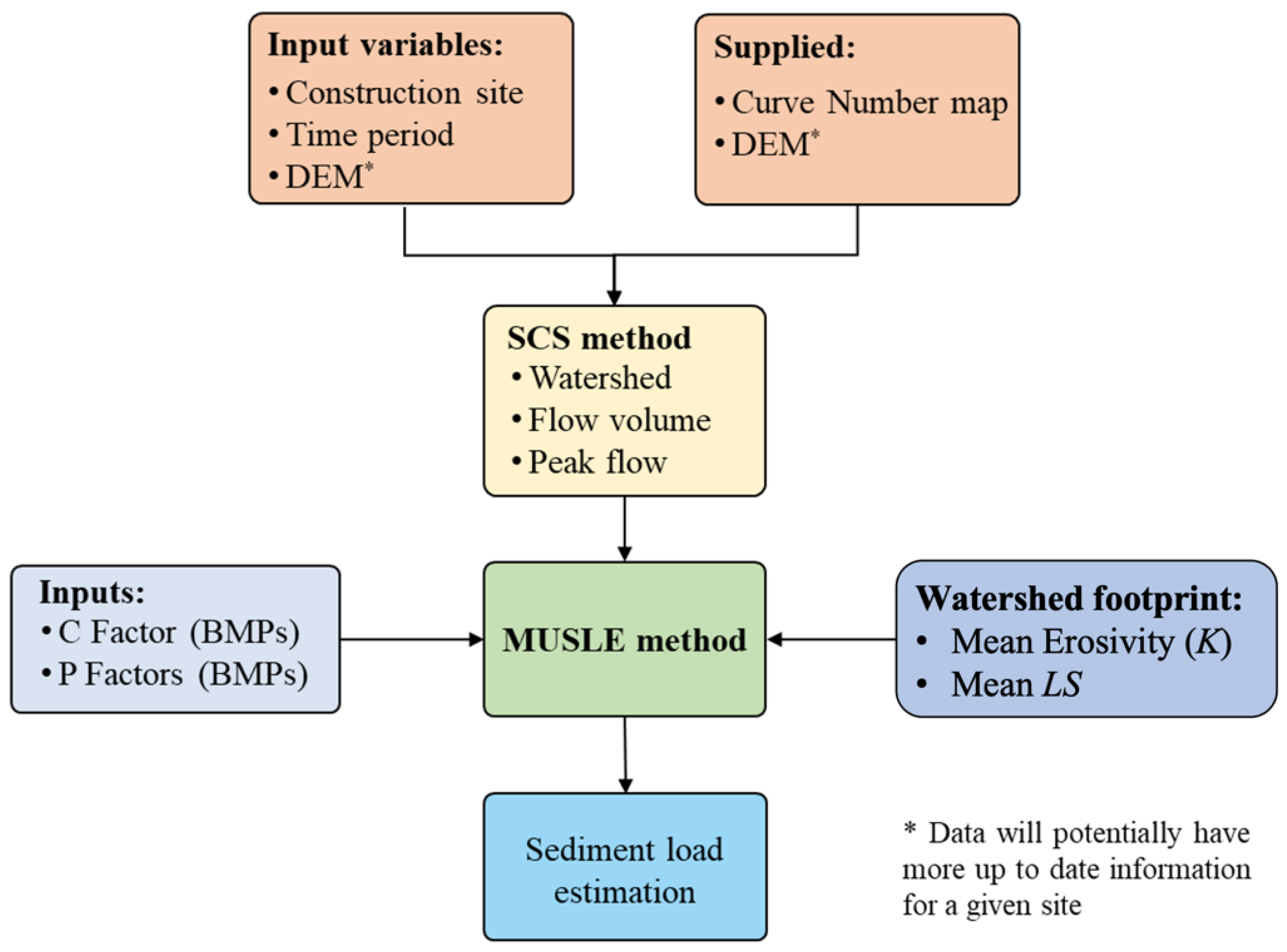
3. Overland Erosion GIS Toolkit
3.1. MUSLE Model
3.2. SCS Method
3.3. Model Inputs
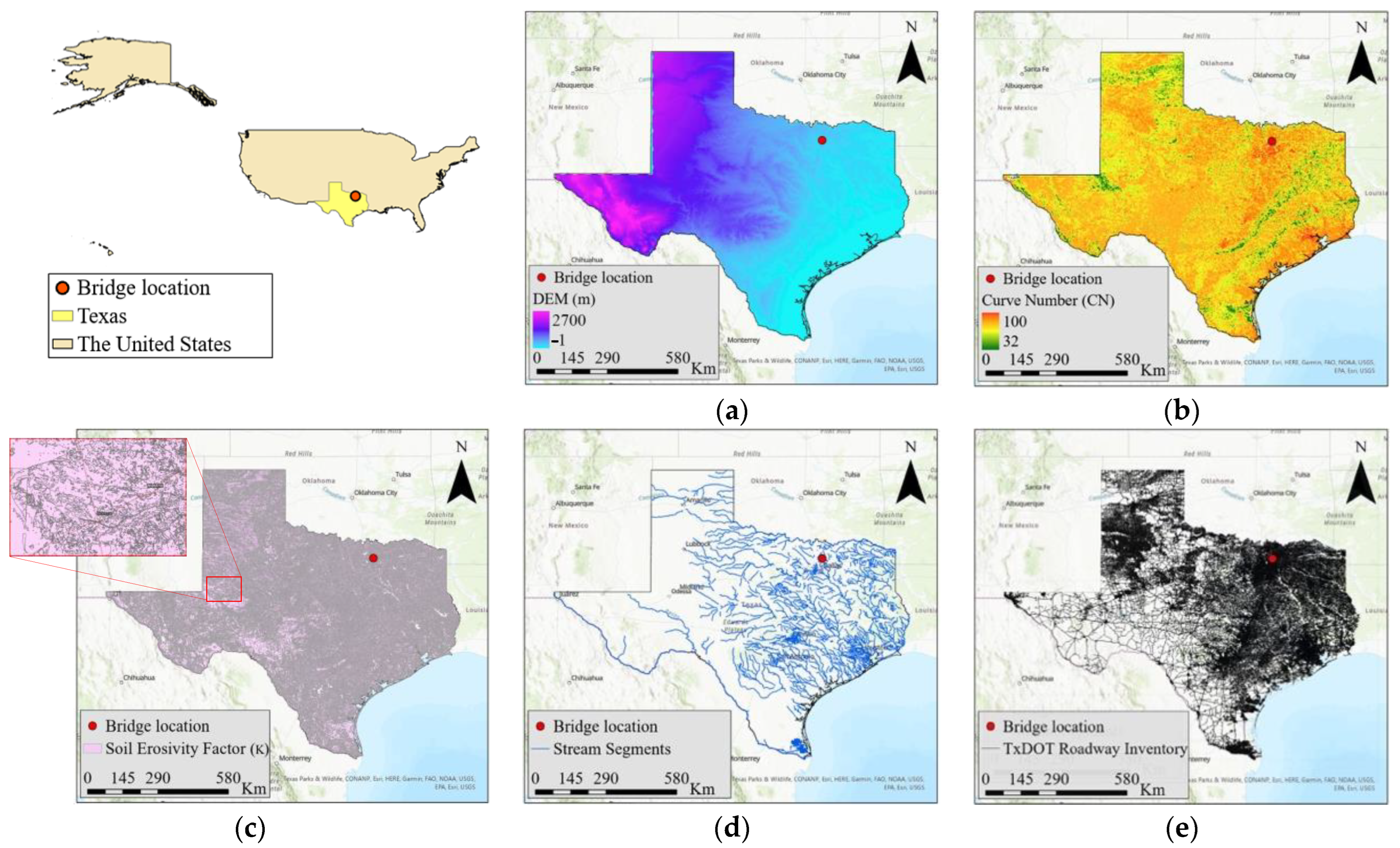
3.3.1. Preloaded Data
- Digital Elevation Model (DEM)
- CurveNumber (CN)
- Soil Erosivity Factor (K)
- Stream Segments
- Road Map Inventory
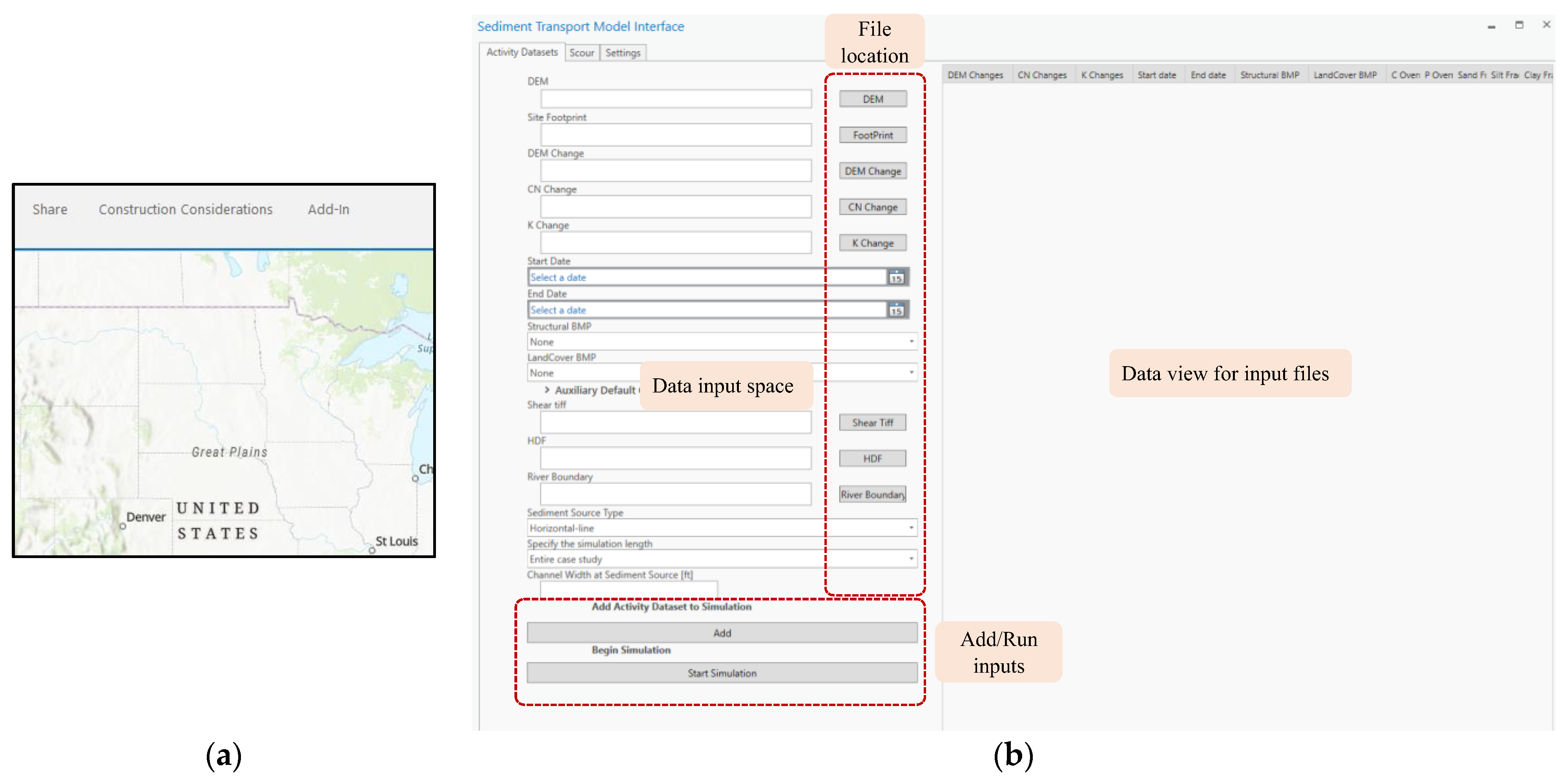
3.3.2. User-Defined Data
- Construction Site Footprint
- Start and End Dates of Construction Activities
- DEM Change
- Curve Number (CN) Change
- Soil Erosivity Factor (K) Change
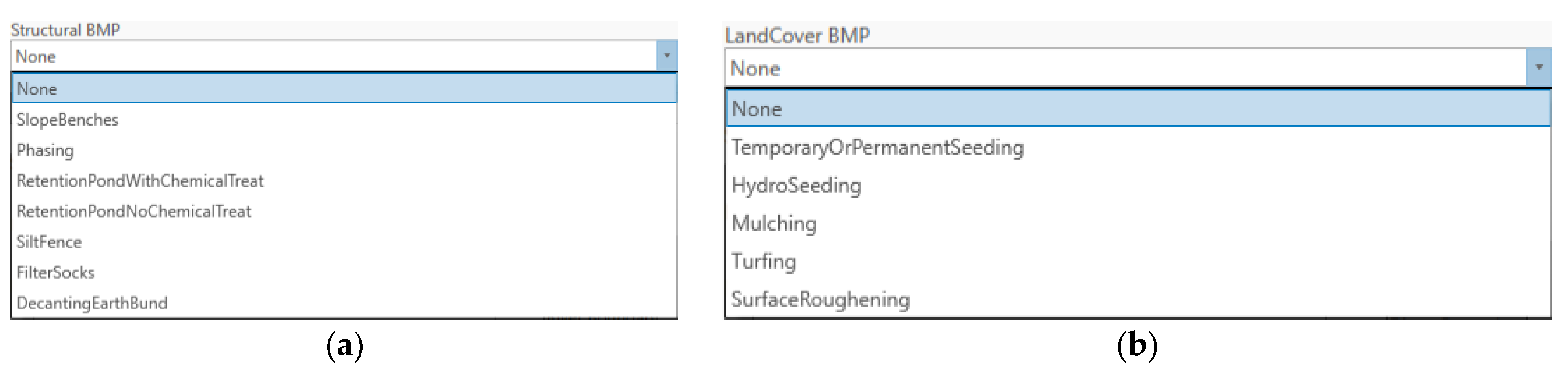
- Best Management Practices (BMPs)
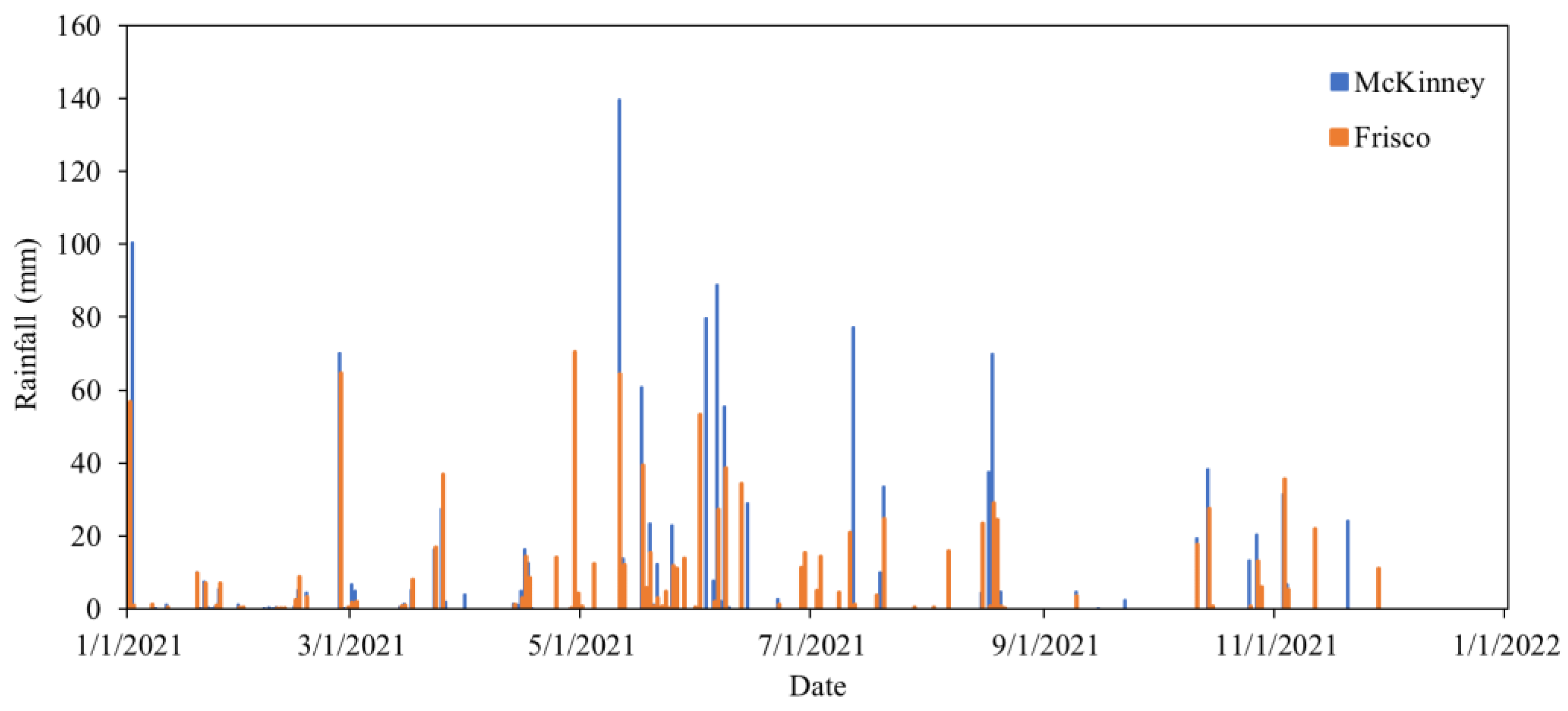
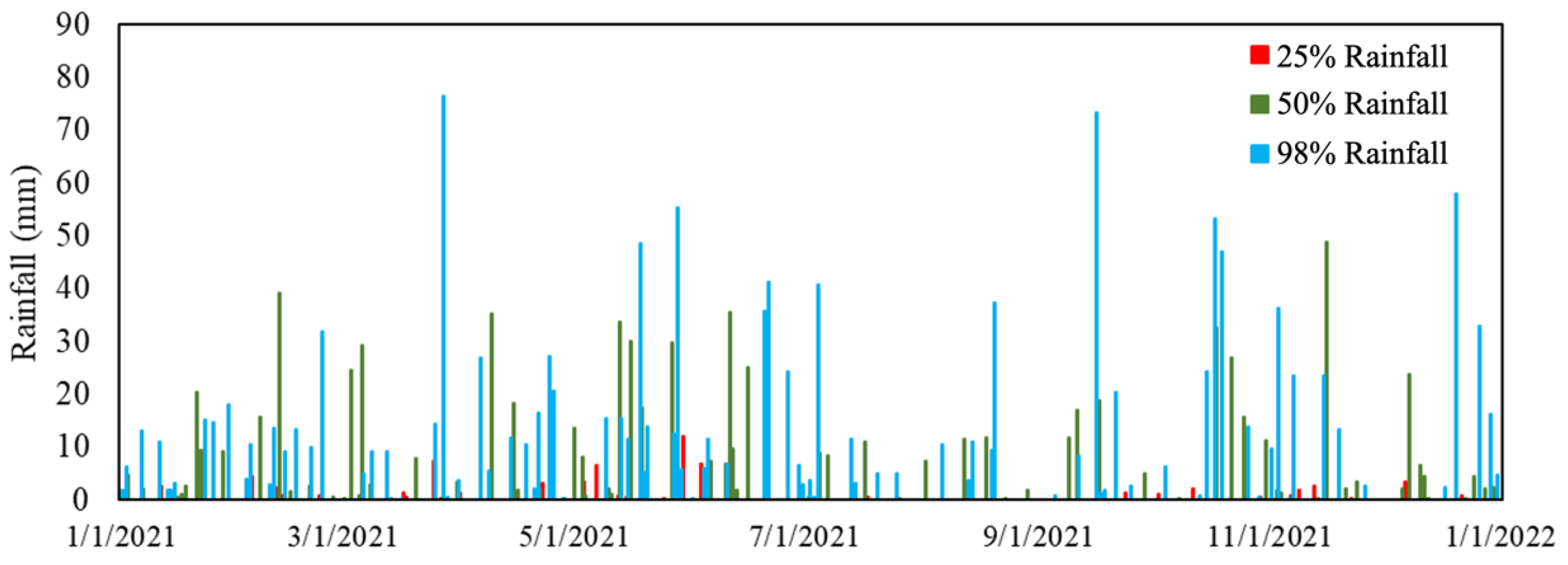
3.4. Rainfall Data
3.4.1. Rain Gauge Station Selection
3.4.2. Rainfall Synthesis Methodology
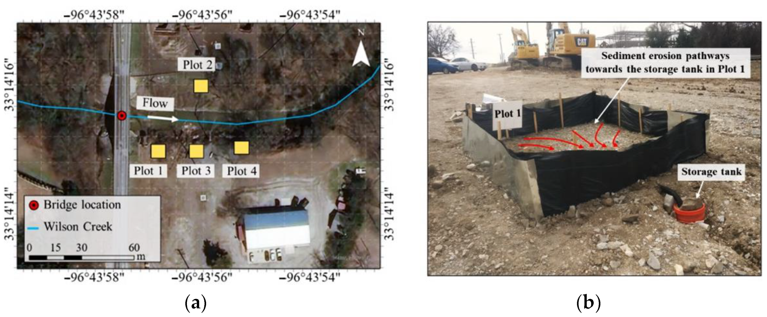
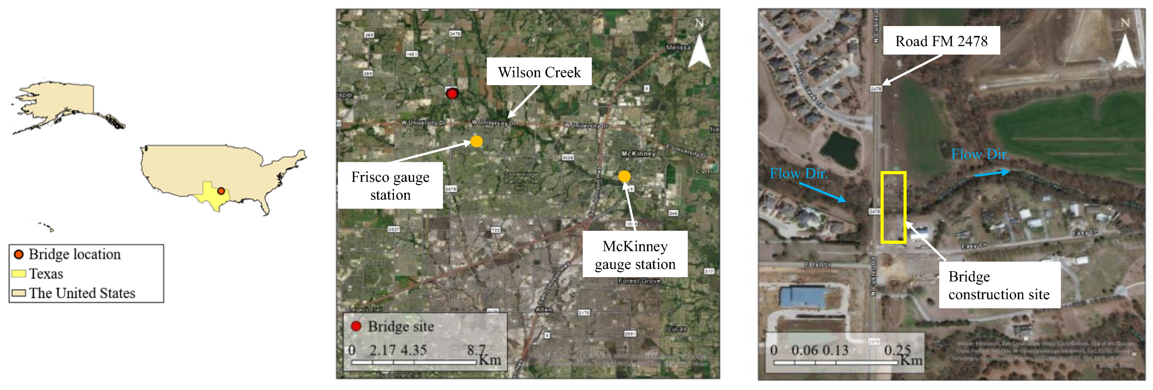
4. Study Area
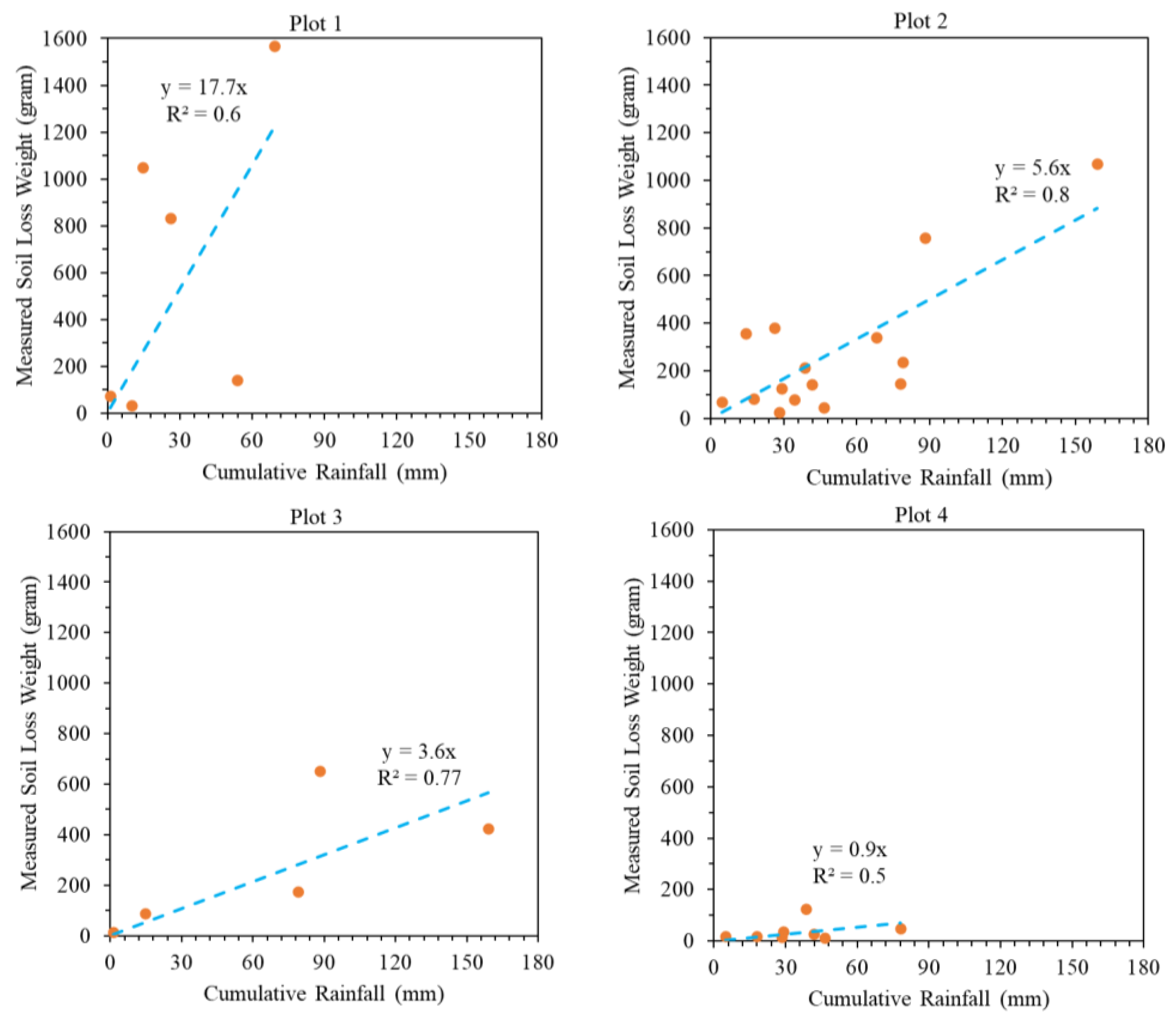
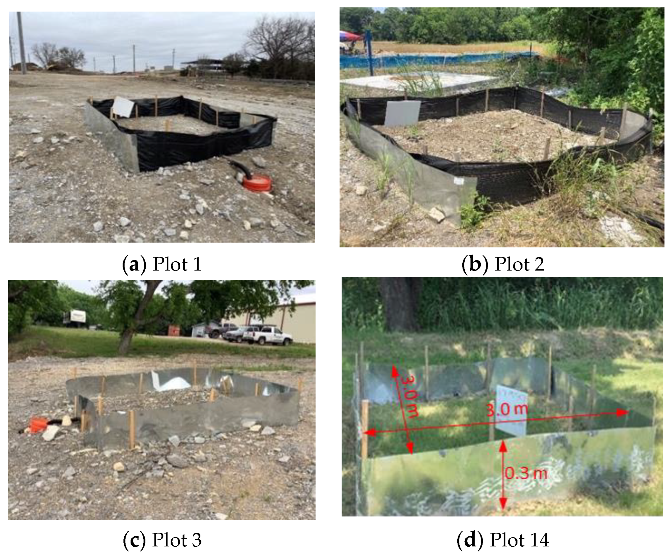
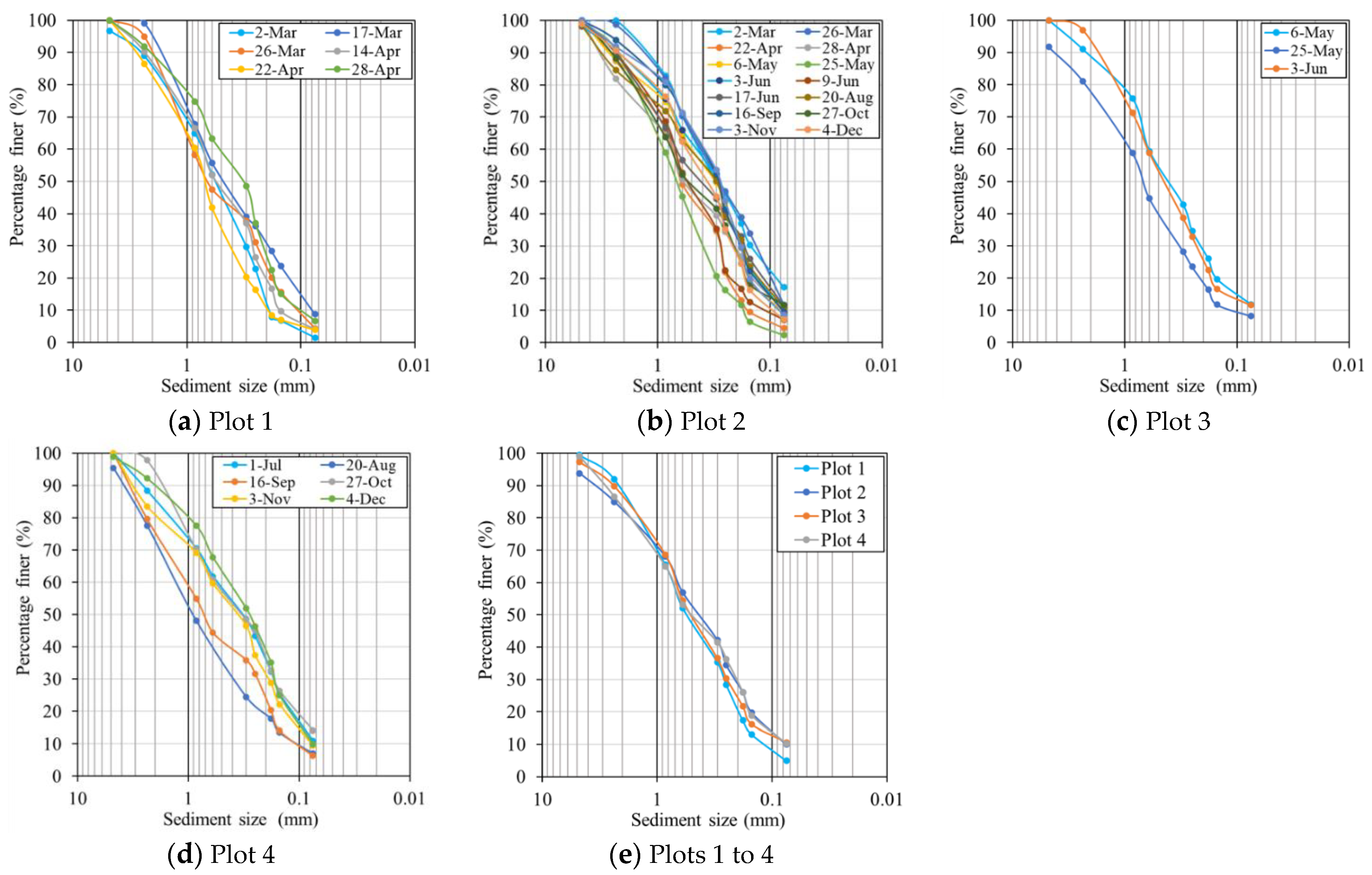
5. Field Monitoring
- Erosion Plot 1
- Erosion Plot 2
- Erosion Plot 3
- Erosion Plot 4
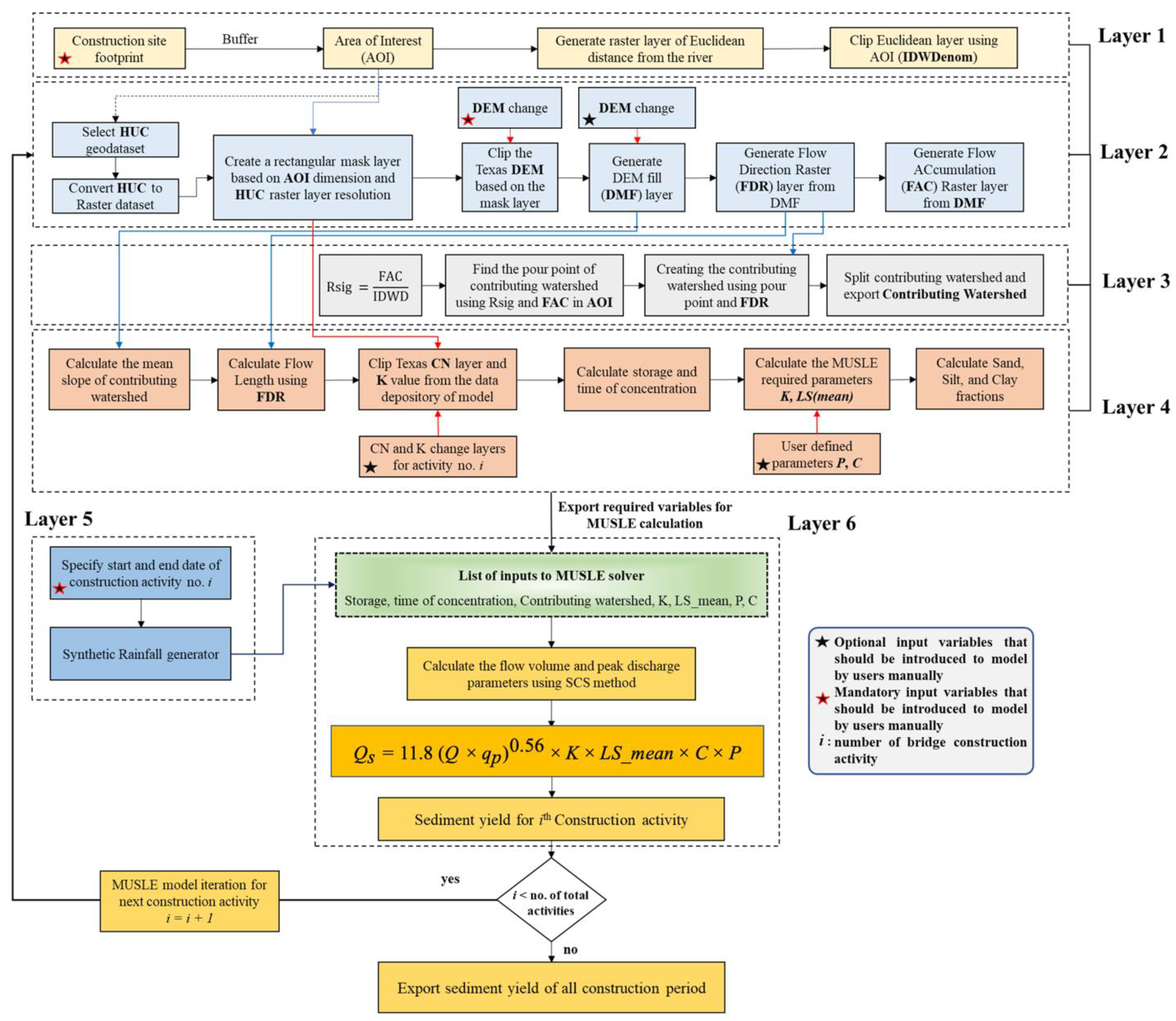
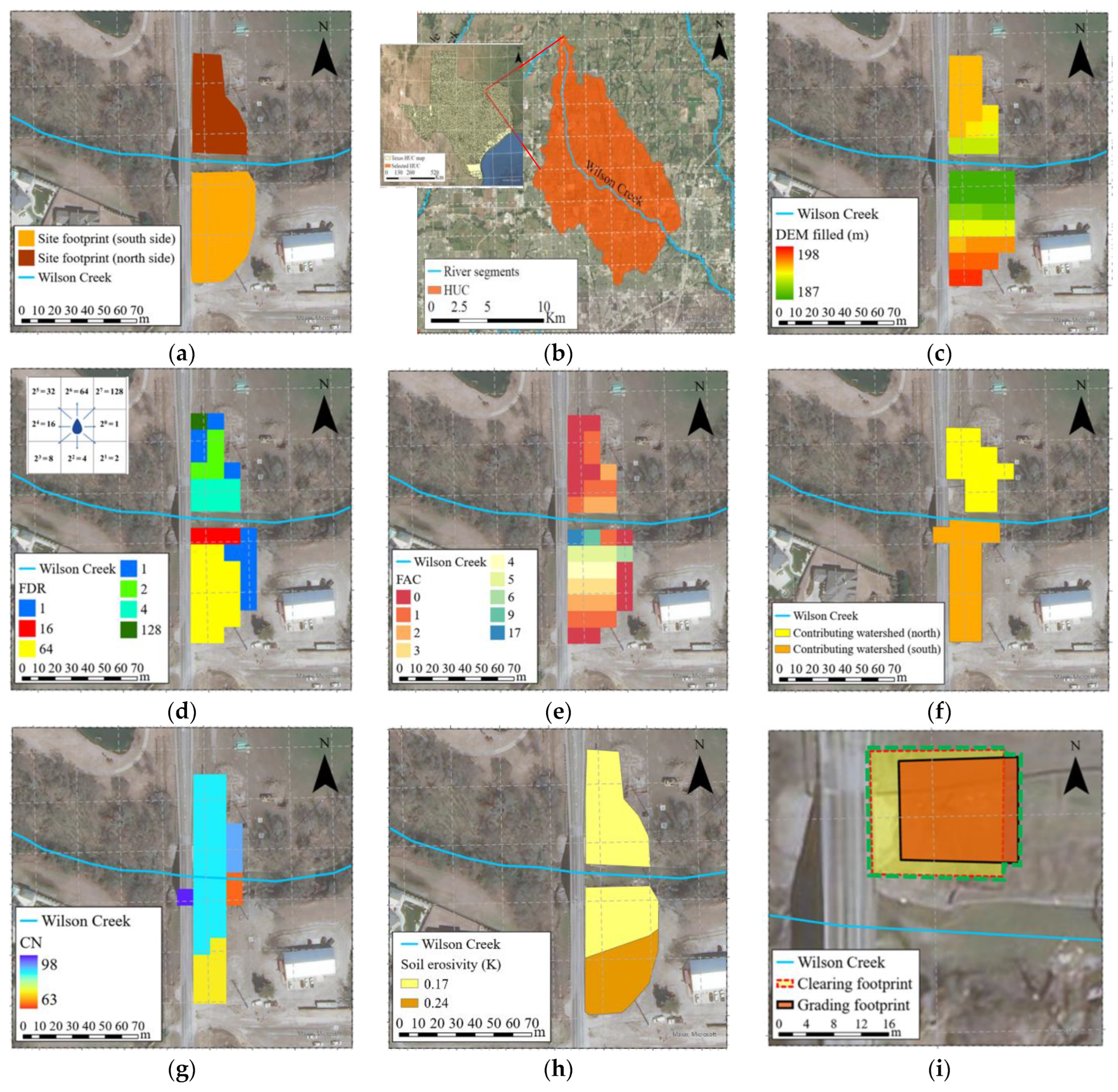
6. Wilson Creek Bridge Construction Site Overland Erosion Model
Model Setup
- Layer 1: Site Footprint
- Layer 2: Sub-watershed Selection Process
- Layer 3: Creating Contributing Watershed
- Layer 4: Calculating Hydrologic and Watershed Components
- Layer 5: Construction Activity Duration and Rainfall Generator
- Layer 6: MUSLE Model
7. Assessment of Overland Erosion Model Performance
7.1. Model Results for Without-Construction Scenario
7.2. Comparison with Universal Soil Loss Equation (USLE) Method
7.3. Comparison with Soil Loss from Erosion Plots
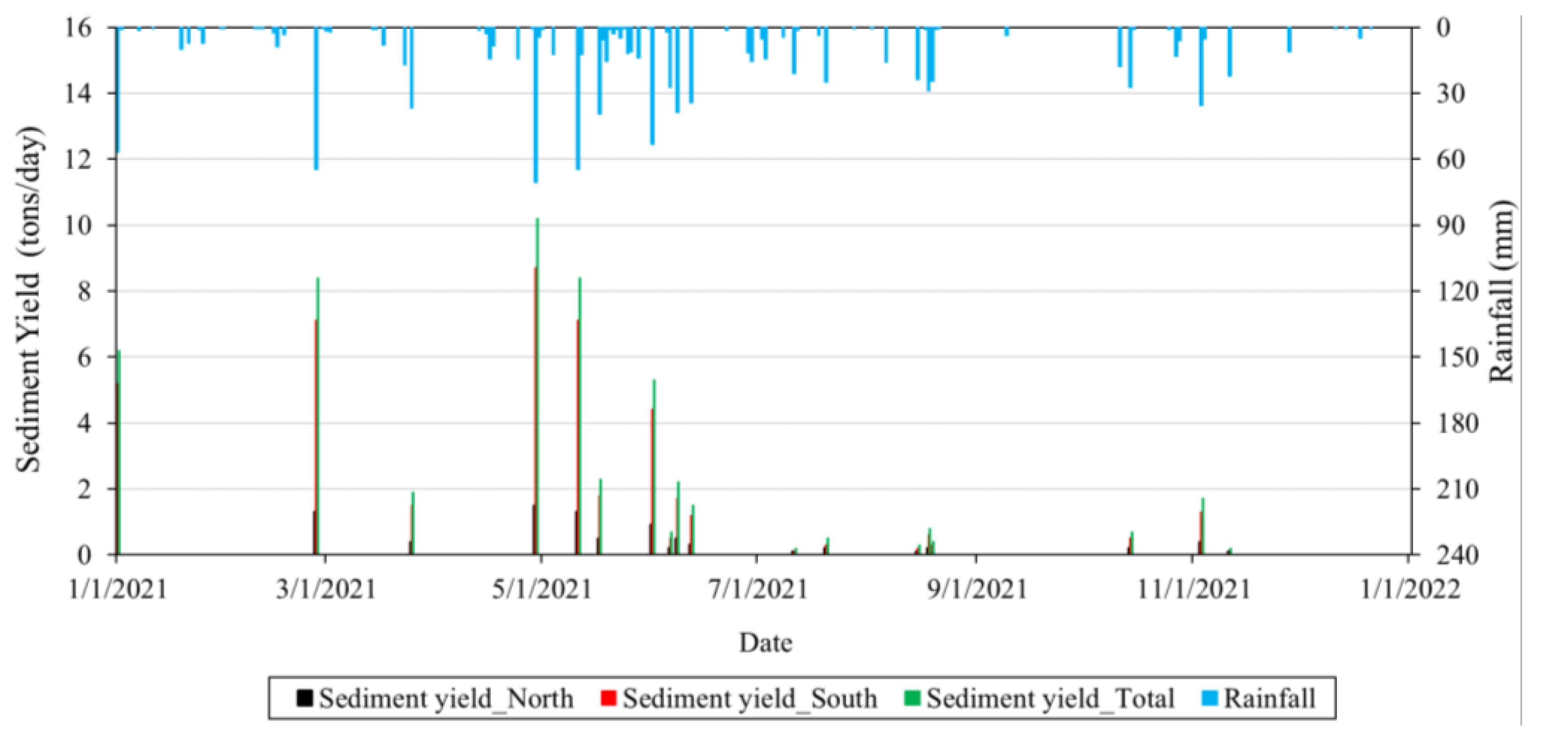
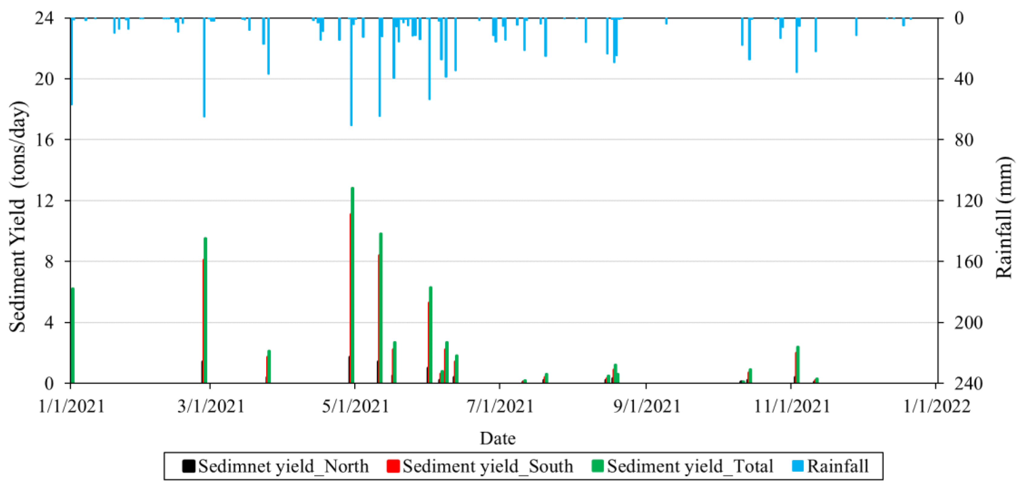
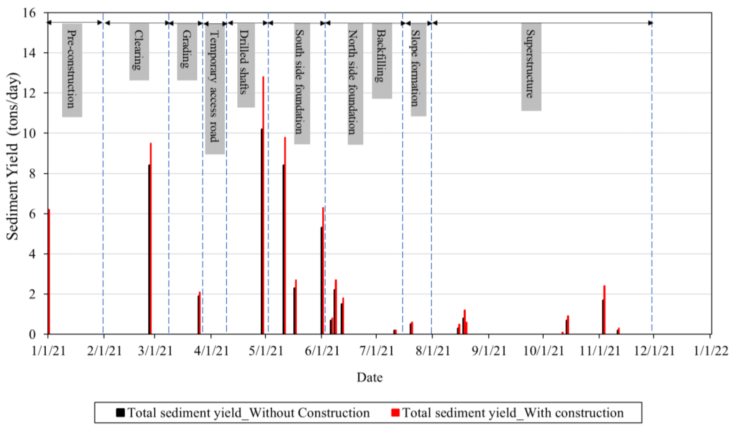
8. Effects of Bridge Construction on Overland Soil Erosion
9. Discussion
9.1. Comparison with Soil Erosion from Other Construction Sites
9.2. Limitations of the Model and Future Direction
10. Conclusions
Author Contributions
Funding
Data Availability Statement
Acknowledgments
Conflicts of Interest
References
- IHS Markit. Critical Infrastructure for Texas Growth. 2019. Available online: https://docs.txoga.org/files/1021-ihs_3-19-19-final.pdf (accessed on 26 August 2022).
- U.S. Environment Protection Agency (EPA). Environmental Impact and Benefits Assessment for Final Effluent Guidelines and Standards for the Construction and Development Category; EPA-821-R-09-012; U.S. Environment Protection Agency (EPA): Washington, DC, USA, 2009.
- Witheridge, G. Erosion and Sediment Control Field Guide for Road Construction-Part 1; Catchments & Creeks Pty Limited: Brisbane, Queensland, Australia, 2017. [Google Scholar]
- Wellman, J.C.; Combs, D.L.; Cook, S.B. Long-term impacts of bridge and culvert construction or replacement on fish communities and sediment characteristics of streams. J. Freshw. Ecol. 2000, 15, 317–328. [Google Scholar] [CrossRef]
- Hedrick, L.B.; Welsh, S.A.; Anderson, J.T. Influences of high-flow events on a stream channel altered by construction of a highway bridge: A case study. Northeast. Nat. 2009, 16, 375–394. [Google Scholar] [CrossRef]
- Weaver, W.; Hagans, D. Road upgrading, decommissioning and maintenance: Estimating costs on small and large scales. In Proceedings of the NMFS Salmonid Habitat Restoration Cost Workshop, Washington, DC, USA, 14–16 November 2000; National Marine Fisheries Service, National Oceanic and Atmospheric Administration, U.S. Department of Commerce: Washington, DC, USA, 2004. [Google Scholar]
- Ahmari, H.; Randklev, C.R.; Jaber, F.; Yu, X.; Baharvand, S.; Pebworth, M.; Kandel, S.; Goldsmith, A.M. Determining Downstream Ecological Impacts of Sediment Derived from Bridge Construction; TxDOT Report No. 0-7023; Texas Department of Transportation: Downtown Austin, TX, USA, 2022. [Google Scholar]
- Mendonça dos Santos, F.; Proença de Oliveira, R.; Augusto Di Lollo, J. Effects of Land Use Changes on Streamflow and Sediment Yield in Atibaia River Basin—SP, Brazil. Water 2020, 12, 1711. [Google Scholar] [CrossRef]
- Németová, Z.; Honek, D.; Kohnová, S.; Hlavčová, K.; Šulc Michalková, M.; Sočuvka, V.; Velísková, Y. Validation of the EROSION-3D model through measured bathymetric sediments. Water 2020, 12, 1082. [Google Scholar] [CrossRef]
- Sharma, K.D.; Singh, S. Satellite remote sensing for soil erosion modelling using the ANSWERS model. Hydrol. Sci. J. 1995, 40, 259–272. [Google Scholar] [CrossRef]
- Zhang, Y.; Degroote, J.; Wolter, C.; Sugumaran, R. Integration of modified universal soil loss equation (MUSLE) into a GIS framework to assess soil erosion risk. Land Degrad. Dev. 2009, 20, 84–91. [Google Scholar] [CrossRef]
- Ohio Department of Natural Resources (ODNR). Ohio Mussel Survey Protocol. Division of Wildlife and U.S. Fish and Wildlife Service (USFWS); Ohio Ecological Services Field Office: Columbus, OH, USA, 2020.
- Virginia Department of Game and Inland Fisheries (VDGIF) and the U.S. Fish and Wildlife Service (FWS). Freshwater Mussels Guideline for Virginia; 2018. Available online: https://dwr.virginia.gov/wp-content/uploads/mussel-guidelines-11-2018.pdf (accessed on 26 August 2022).
- U.S. Fish and Wildlife Service (USFWS); Ecological Services and Fisheries Resources Offices and Georgia Department of Transportation; Office of Environment and Location. Freshwater Mussel Survey Protocol for the Southeastern Atlantic Slope and Northeastern Gulf Drainages in Florida and Georgia; 2008. Available online: https://www.fws.gov/sites/default/files/documents/Final-Mussel-Survey-Protocol-FL-GA-April-2008.pdf (accessed on 26 August 2022).
- U.S. Fish and Wildlife Service Texas Ecological Services Field Offices and Texas Parks and Wildlife Department. Texas Freshwater Mussel Survey Protocol; 2021. Available online: https://www.fws.gov/sites/default/files/documents/2021_Texas_Freshwater_Mussel_Survey_Protocol.pdf (accessed on 26 August 2022).
- Weaver, W.E.; Hagans, D.K. Handbook for Forest and Ranch Roads: A Guide for Planning, Designing, Constructing, Reconstructing, Maintaining and Closing Wildland Roads; Pacific Watershed Associates: Arcata, CA, USA, 1994. [Google Scholar]
- U.S. Department of Agriculture (USDA). Erosion and Sedimentation on Construction Sites, Soil Quality-Urban Technical Note; No.1; Soil Quality Institute: Auburn, AL, USA, 2000.
- Merritt, W.S.; Letcher, R.A.; Jakeman, A.J. A review of erosion and sediment transport models. Environ. Model. Softw. 2003, 18, 761–799. [Google Scholar] [CrossRef]
- Alewell, C.; Borrelli, P.; Meusburger, K.; Panagos, P. Using the USLE: Chances, challenges and limitations of soil erosion modelling. Int. Soil Water Conserv. Res. 2019, 7, 203–225. [Google Scholar] [CrossRef]
- Roose, E. Land Husbandry-Components and Strategy; FAO Soils Bulletin: Rome, Italy, 1996; Volume 70. [Google Scholar]
- Construction General Permit. Proposed Construction General Permit (CGP) 2017. Available online: https://www3.epa.gov/npdes/pubs/cgp_appendixh.pdf (accessed on 17 October 2019).
- Yang, C.T. Erosion and Sedimentation Manual; U.S. Department of the Interior, Bureau of Reclamation: Denver, CO, USA, 2006. [Google Scholar]
- Brevik, E.C.; Pereira, P.; Muñoz-Rojas, M.; Miller, B.A.; Cerdà, A.; Parras-Alcántara, L.; Lozano-García, B. Historical Perspectives on Soil Mapping and Process Modeling for Sustainable Land Use Management. In Soil Mapping and Process Modeling for Sustainable Land Use Management; Elsevier: Amsterdam, The Netherlands, 2017; pp. 3–28. [Google Scholar]
- U.S. Department of Agriculture (USDA). Revised Universal Soil Loss Equation Version 2 (RUSLE2) (for the Model with Release Date of 20 May 2008); Science Documentation; USDA-Agricultural Research Service: Washington, DC, USA, 2013.
- Smith, S.J.; Williams, J.R.; Menzel, R.G.; Coleman, G.A. Prediction of Sediment Yield from Southern Plains Grasslands with the Modified Universal Soil Loss Equation. J. Range Manag. 1984, 37, 295. [Google Scholar] [CrossRef]
- Younkin, L.M. Effects of Highways Construction on Sediment Loads in Streams. In Soil Erosion: Causes and Mechanisms: Prevention and Control; Washington, DC, USA, 1973; Volume 135, pp. 82–93. Available online: http://onlinepubs.trb.org/Onlinepubs/sr/sr135/sr135-008.pdf (accessed on 17 October 2019).
- Reed, L.A.; Ward, J.R.; Wetzel, K.L. Calculating Sediment Discharge from a Highway Construction Site in Central Pennsylvania; U.S. Geological Survey, Pennsylvania Water Science Center: New Cumberland, PA, USA, 1985. [Google Scholar] [CrossRef]
- Bouraoui, F.; Dillaha, T.A. ANSWERS-2000: Runoff and Sediment Transport Model. J. Environ. Eng. 1996, 122, 493–502. [Google Scholar] [CrossRef]
- Morgan RP, C.; Quinton, J.N.; Smith, R.E.; Govers, G.; Poesen JW, A.; Auerswald, K.; Chisci, G.; Torri, D.; Styczen, M.E. The European Soil Erosion Model (EUROSEM): A dynamic approach for predicting sediment transport from fields and small catchments. Earth Surf. Processes Landf. J. Br. Geomorphol. Group 1998, 23, 527–544. [Google Scholar] [CrossRef]
- Nearing, M.A.; Deer-Ascough, L.; Laflen, J.M. Sensitivity analysis of the WEPP hillslope profile erosion model. Trans. ASAE 1990, 33, 839–849. [Google Scholar] [CrossRef]
- Neitsch, S.L.; Arnold, J.G.; Kiniry, J.R.; Williams, J.R. Soil and Water Assessment Tool Theoretical Documentation Version 2009. Texas A&M University System: College Station, TX, USA, 2011. [Google Scholar]
- Sadeghi, S.H.R.; Gholami, L.; Khaledi Darvishan, A.; Saeidi, P. A review of the application of the MUSLE model worldwide. Hydrol. Sci. J. 2014, 59, 365–375. [Google Scholar] [CrossRef]
- Williams, J.R.; Berndt, H.D. Sediment yield prediction based on watershed hydrology. Trans. ASAE 1977, 20, 1100–1104. [Google Scholar] [CrossRef]
- Pongsai, S.; Schmidt Vogt, D.; Shrestha, R.P.; Clemente, R.S.; Eiumnoh, A. Calibration and validation of the Modified Universal Soil Loss Equation for estimating sediment yield on sloping plots: A case study in Khun Satan catchment of northern Thailand. Can. J. Soil Sci. 2010, 90, 585–596. [Google Scholar] [CrossRef]
- Mays, L.W. Water Resources Engineering, 2nd ed.; John Wiley & Sons: Hoboken, NJ, USA, 2010. [Google Scholar]
- U.S. Department of Agriculture (USDA). Revised Universal Soil Loss Equation 2-How RUSLE2 Computes Rill and Interrill Erosion. (n.d.). Available online: https://www.ars.usda.gov/southeast-area/oxford-ms/national-sedimentation-laboratory/watershed-physical-processes-research/research/rusle2/revised-universal-soil-loss-equation-2-how-rusle2-computes-rill-and-interrill-erosion/ (accessed on 17 October 2019).
- Tillman, F.D.; Flynn, M.E.; Anning, D.W. Geospatial Datasets for Assessing the Effects of Rangeland Conditions on Dissolved-Solids Yields in the Upper Colorado River Basin; No. 2015-1007; U.S. Geological Survey: Washington, DC, USA, 2015. [Google Scholar]
- U.S. Department of Agriculture (USDA). Soil Survey Geographic (SSURGO) Database. Available online: https://www.nrcs.usda.gov/wps/portal/nrcs/detail/soils/survey/geo/?cid=nrcs142p2_053631. (accessed on 26 August 2022).
- Texas Commission on Environmental Quality (TCEQ) Open Data Portal. 2019. Available online: https://gis-tceq.opendata.arcgis.com/datasets/segments-poly?geometry=-154.658,24.504,-42.905,37.629. (accessed on 22 November 2019).
- Texas Department of Transportation (TxDOT). TxDOT Roadways Inventory. Available online: https://gis-txdot.opendata.arcgis.com/datasets/843ebe994c114961a855ec76ddcde086_0/explore?location=31.061298%2C-100.081515%2C6.88. (accessed on 26 August 2022).
- National Oceanic and Atmosphieric Adminestration (NOAA). National Centers for Environmental Information. Global Historical Climatology Network daily (GHCNd). Available online: https://www.ncei.noaa.gov/products/land-based-station/global-historical-climatology-network-daily. (accessed on 26 August 2022).
- Singh, V.P. Pearson Type III Distribution. In Entropy-Based Parameter Estimation in Hydrology; Springer: Dordrecht, The Netherlands, 1998; Volume 30, pp. 252–274. [Google Scholar]
- Grimaldi, S.; Kao, S.-C.; Castellarin, A.; Papalexiou, S.-M.; Viglione, A.; Laio, F.; Aksoy, H.; Gedikli, A. Statistical Hydrology; Wilderer, P.A., Ed.; Treatise on Water Science, Four-Volume Set (p. 488); Elsevier Science: Amsterdam, The Netherlands, 2011; pp. 479–517. [Google Scholar] [CrossRef]
- Fadhil, R.; Rowshon, M.; Ahmad, D.; Fikri, A.; Aimrun, W. A stochastic rainfall generator model for simulation of daily rainfall events in Kurau catchment: Model testing. Acta Hortic. 2017, 1152, 1–10. [Google Scholar] [CrossRef]
- Tettey, M.; Oduro, F.T.; Adedia, D.; Abaye, D.A. Markov chain analysis of the rainfall patterns of five geographical locations in the southeastern coast of Ghana. Earth Perspect. 2017, 4, 6. [Google Scholar] [CrossRef]
- Ferring, C.R. Late Quaternary Geology of the Upper Trinity River Basin, Texas. Doctoral Dissertation, The University of Texas at Dallas, Richardson, TX, USA, 1994. [Google Scholar]
- Moring, J.B. Effects of Urbanization on the Chemical, Physical, and Biological Characteristics of Small Blackland Prairie Streams in and near the Dallas-Fort Worth Metropolitan Area, Texas; Chapter C in Effects of urbanization on stream ecosystems in six metropolitan areas of the United States (No. 2006-5101-C); U.S. Geological Survey: Washington, DC, USA, 2009. [Google Scholar]
- Harmel, R.D.; Richardson, C.W.; King, K.W.; Allen, P.M. Runoff and soil loss relationships for the Texas Blackland Prairies ecoregion. J. Hydrol. 2006, 331, 471–483. [Google Scholar] [CrossRef]
- Maier, N.D.; Dunkin, J.T. McKinney Floodplain Management Study: Wilson Creek, Franklin Branch, Stover Creek, Honey Creek; Prepared for City of McKinney, Texas; 1988. Available online: https://www.mckinneytexas.org/DocumentCenter/View/408/McKinney-Floodplain-Management-Study-_1988?bidId= (accessed on 13 August 2022).
- American Society for Testing and Materials (ASTM). Standard Practice for Classification of Soils for Engineering Purposes (Unified Soil Classification System. s.l.; ASTM International: West Conshohocken, PA, USA, 2006. [Google Scholar]
- Greiner, J.H. Erosion and Sedimentation by Water in Texas-Average Annual Rates Estimated in 1979; Report Prepared for Texas; Department of Water Resources: Sacramento, CA, USA, 1982. [Google Scholar]
- Hainly, R.A. The effects of highway construction on sediment discharge into Blockhouse Creek and Steam Valley Run; Pennsylvania (No. 80-68); U.S. Geological Survey: Washington, DC, USA, 1980. [Google Scholar]
- U.S. Geological Survey (USGS). POLARIS: A 30-Meter Probabilistic Soil Series Map of the Contiguous United States. Available online: https://pubs.er.usgs.gov/publication/70170912 (accessed on 26 August 2022).


| State | Dry | Wet |
|---|---|---|
| Dry | 0.821 | 0.179 |
| Wet | 0.617 | 0.383 |
| Stable state | 0.775 | 0.225 |
| Construction Activity | Date | BMPs | |
|---|---|---|---|
| Start | End | ||
| Site clearing | 1 February 2021 | 10 March 2021 | Silt fence-north side |
| Grading | 11 March 2021 | 26 March 2021 | Silt fence-north side |
| Temporary access road | 27 March 2021 | 10 April 2021 | Silt curtain and rock trap across the creek |
| Drilled shafts | 11 April 2021 | 3 May 2021 | Silt fence along the creek edge on both sides/Rock trap |
| Foundations/piers/abutments Southside Northside | 4 May 2021 3 June 2021 | 2 June 2021 14 July 2021 | Silt fence along the creek edge on both sides (after 15 May)/Rock trap (until 29 May)/Vegetation BMPs on the south side (from 3 June) |
| Backfilling | 3 June 2021 | 14 July 2021 | Silt fence along the creek edge on both sides/Vegetation BMPs on the south side |
| Slope formation | 15 July 2021 | 29 July 2021 | Vegetation BMPs on south side/Rock trap |
| Superstructure | 30 July 2021 | 30 November 2021 | Vegetation BMPs on south side/Rock trap |
| Sediment Class | Ave. Diameter (mm) | Fraction (%) | |
|---|---|---|---|
| North | South | ||
| Sand | 0.25 | 9 | 10 |
| Silt | 0.016 | 21 | 32 |
| Clay | 0.002 | 70 | 58 |
| Site | R | K | LS | C | P | Soil Loss, A 1 (kg/m2/Year) | Sediment Yield 2 (kg/m2/Year) | Sediment Delivery Ratio (%) |
|---|---|---|---|---|---|---|---|---|
| North | 295 | 0.17 | 0.7 | 1 | 1 | 8.7 | 5.8 | 66 |
| South | 295 | 0.2 | 4.11 | 1 | 1 | 59.9 | 18.5 | 31 |
Publisher’s Note: MDPI stays neutral with regard to jurisdictional claims in published maps and institutional affiliations. |
© 2022 by the authors. Licensee MDPI, Basel, Switzerland. This article is an open access article distributed under the terms and conditions of the Creative Commons Attribution (CC BY) license (https://creativecommons.org/licenses/by/4.0/).
Share and Cite
Ahmari, H.; Pebworth, M.; Baharvand, S.; Kandel, S.; Yu, X. Development of an ArcGIS-Pro Toolkit for Assessing the Effects of Bridge Construction on Overland Soil Erosion. Land 2022, 11, 1586. https://doi.org/10.3390/land11091586
Ahmari H, Pebworth M, Baharvand S, Kandel S, Yu X. Development of an ArcGIS-Pro Toolkit for Assessing the Effects of Bridge Construction on Overland Soil Erosion. Land. 2022; 11(9):1586. https://doi.org/10.3390/land11091586
Chicago/Turabian StyleAhmari, Habib, Matthew Pebworth, Saman Baharvand, Subhas Kandel, and Xinbao Yu. 2022. "Development of an ArcGIS-Pro Toolkit for Assessing the Effects of Bridge Construction on Overland Soil Erosion" Land 11, no. 9: 1586. https://doi.org/10.3390/land11091586
APA StyleAhmari, H., Pebworth, M., Baharvand, S., Kandel, S., & Yu, X. (2022). Development of an ArcGIS-Pro Toolkit for Assessing the Effects of Bridge Construction on Overland Soil Erosion. Land, 11(9), 1586. https://doi.org/10.3390/land11091586