
Evaluation of Accuracy Enhancement in European-Wide Crop Type Mapping by Combining Optical and Microwave Time Series


Abstract
:1. Introduction
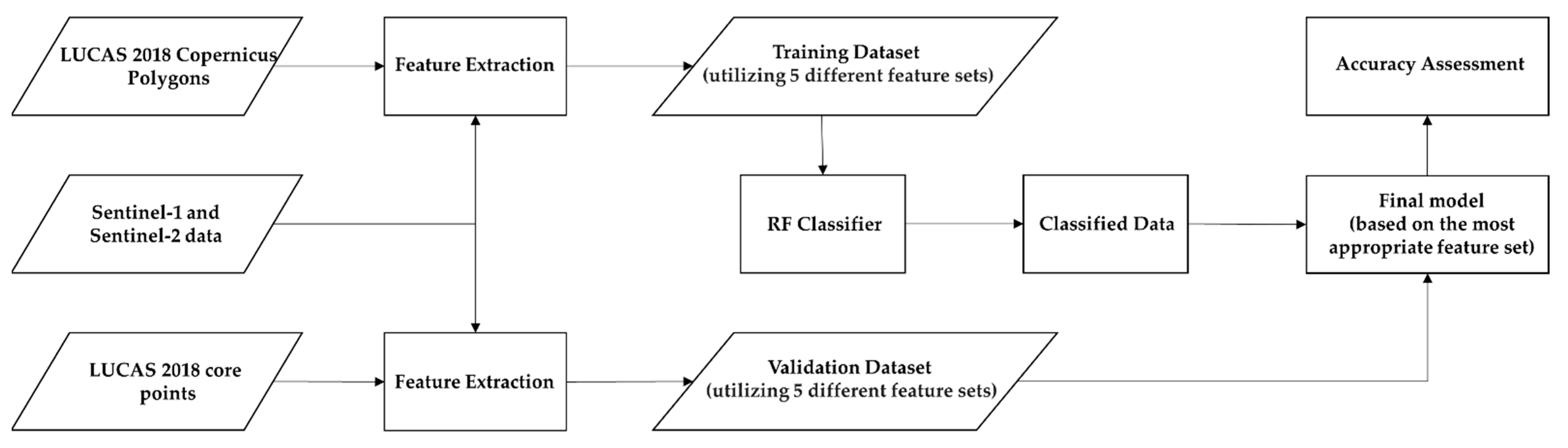
2. Materials and Methods
2.1. Training Data Preparation
2.1.1. LUCAS 2018 Data
2.1.2. Classification Scheme Based on LUCAS 2018 Data
2.2. Earth Observation Data
2.2.1. Sentinel-2 Data Preparation
2.2.2. Sentinel-1 Data Preparation
- Edge masking: The edge of each scene was masked by groups of adjacent pixels with values lesser than 25 decibels (dB) in the VV polarization.
- Averaging of 10 days: σ0 natural values were averaged over the following periods of 10 days for each pixel for all available ascending and descending acquisitions, separately for the VV and VH polarizations. The averaged σ0 value was then transformed to dB.
- Computing the CR ratio: The CR was calculated and averaged for each scene for the same 10-day period.
2.3. Sentinel-1 and Sentinel-2 Features for the LUCAS Copernicus Polygons
2.4. Classification Process: The Classifier, Validation Data, and Assessment Metrics
3. Results
4. Discussion
5. Conclusions
Author Contributions
Funding
Institutional Review Board Statement
Informed Consent Statement
Data Availability Statement
Acknowledgments
Conflicts of Interest
Appendix A

| Code | (211) Common Wheat | (212) Durum Wheat | (213) Barley | (214) Rye | (215) Oats | (216) Maize | (217) Rice | (218) Triticale | (219) Other Cereals | (221) Potatoes | (222) Sugar Beet | (223) Other Root Crops | (230) Other Non-Permanent | (231) Sunflower | (232) Rape and Turnip Rape | (233) Soya | (240) Dry Pulses, Vegetables, | (250) Fodder Crops | (290) Bare Arable Land | (300) Woodland and Shrubland | (500) Grassland | Total | UA (%) | F1-Score (%) |
|---|---|---|---|---|---|---|---|---|---|---|---|---|---|---|---|---|---|---|---|---|---|---|---|---|
| 211 | 4340 | 405 | 890 | 308 | 298 | 76 | 9 | 276 | 18 | 16 | 10 | 11 | 44 | 4 | 102 | 2 | 62 | 150 | 631 | 19 | 510 | 8181 | 53.0 | 63.9 |
| 212 | 35 | 305 | 24 | 1 | 17 | 0 | 0 | 1 | 0 | 0 | 0 | 0 | 0 | 0 | 0 | 0 | 2 | 25 | 16 | 0 | 19 | 445 | 68.5 | 38.6 |
| 213 | 319 | 97 | 1773 | 91 | 189 | 6 | 13 | 35 | 1 | 2 | 0 | 8 | 28 | 0 | 25 | 0 | 69 | 105 | 205 | 8 | 182 | 3156 | 56.2 | 54.5 |
| 214 | 12 | 0 | 14 | 127 | 5 | 2 | 0 | 41 | 0 | 2 | 0 | 0 | 2 | 0 | 2 | 0 | 2 | 0 | 6 | 1 | 8 | 224 | 56.7 | 27.5 |
| 215 | 8 | 0 | 13 | 4 | 32 | 0 | 0 | 0 | 1 | 0 | 0 | 0 | 0 | 0 | 0 | 0 | 0 | 6 | 5 | 0 | 6 | 75 | 42.7 | 7.3 |
| 216 | 63 | 14 | 51 | 13 | 15 | 3331 | 49 | 7 | 59 | 93 | 24 | 22 | 42 | 38 | 3 | 68 | 92 | 48 | 94 | 14 | 200 | 4340 | 76.8 | 82.1 |
| 217 | 0 | 0 | 0 | 0 | 0 | 0 | 3 | 0 | 0 | 0 | 0 | 0 | 0 | 0 | 0 | 0 | 0 | 0 | 1 | 0 | 0 | 4 | 75.0 | 6.1 |
| 218 | 0 | 0 | 0 | 0 | 0 | 0 | 0 | 0 | 0 | 0 | 0 | 0 | 0 | 0 | 0 | 0 | 0 | 0 | 0 | 0 | 0 | 0 | 0.0 | 0.0 |
| 219 | 0 | 0 | 0 | 0 | 0 | 0 | 0 | 0 | 0 | 0 | 0 | 0 | 0 | 0 | 0 | 0 | 0 | 0 | 0 | 0 | 0 | 0 | 0.0 | 0.0 |
| 221 | 0 | 0 | 0 | 0 | 0 | 1 | 0 | 1 | 0 | 225 | 5 | 2 | 4 | 1 | 0 | 7 | 12 | 0 | 5 | 0 | 2 | 265 | 84.9 | 67.4 |
| 222 | 2 | 0 | 5 | 1 | 1 | 5 | 1 | 0 | 1 | 10 | 577 | 14 | 3 | 4 | 1 | 0 | 21 | 1 | 3 | 0 | 4 | 654 | 88.2 | 88.3 |
| 223 | 0 | 0 | 0 | 0 | 0 | 0 | 0 | 0 | 0 | 0 | 0 | 1 | 0 | 0 | 0 | 0 | 0 | 0 | 1 | 0 | 0 | 2 | 50.0 | 2.0 |
| 230 | 0 | 0 | 0 | 0 | 0 | 0 | 0 | 0 | 0 | 0 | 0 | 0 | 103 | 0 | 0 | 0 | 2 | 1 | 4 | 0 | 0 | 110 | 93.6 | 46.5 |
| 231 | 1 | 1 | 1 | 0 | 2 | 9 | 0 | 0 | 0 | 17 | 2 | 1 | 21 | 535 | 2 | 9 | 33 | 6 | 29 | 0 | 34 | 703 | 76.1 | 79.6 |
| 232 | 11 | 1 | 8 | 1 | 0 | 6 | 0 | 2 | 2 | 1 | 6 | 2 | 5 | 2 | 1303 | 1 | 20 | 6 | 102 | 3 | 57 | 1539 | 84.7 | 84.0 |
| 233 | 0 | 0 | 0 | 0 | 0 | 0 | 0 | 0 | 0 | 0 | 0 | 0 | 1 | 0 | 0 | 60 | 0 | 0 | 2 | 0 | 1 | 64 | 93.8 | 51.5 |
| 240 | 3 | 7 | 4 | 0 | 0 | 1 | 1 | 0 | 2 | 13 | 8 | 13 | 7 | 1 | 15 | 2 | 193 | 19 | 53 | 2 | 34 | 378 | 51.1 | 35.1 |
| 250 | 2 | 1 | 1 | 0 | 3 | 0 | 0 | 0 | 0 | 0 | 0 | 0 | 0 | 0 | 0 | 0 | 6 | 178 | 1 | 0 | 15 | 207 | 86.0 | 15.7 |
| 290 | 4 | 5 | 14 | 0 | 4 | 1 | 0 | 0 | 0 | 3 | 1 | 4 | 2 | 3 | 13 | 0 | 16 | 2 | 612 | 11 | 141 | 836 | 73.2 | 39.5 |
| 300 | 133 | 67 | 121 | 27 | 33 | 114 | 5 | 18 | 12 | 9 | 11 | 2 | 22 | 24 | 29 | 4 | 43 | 113 | 217 | 30,473 | 4027 | 35,504 | 85.8 | 90.5 |
| 500 | 468 | 231 | 436 | 128 | 204 | 226 | 14 | 73 | 38 | 12 | 9 | 17 | 49 | 30 | 68 | 16 | 150 | 1398 | 274 | 1293 | 19,627 | 24,761 | 79.3 | 79.1 |
| Total | 5401 | 1134 | 3355 | 701 | 803 | 3778 | 95 | 454 | 134 | 403 | 653 | 97 | 333 | 642 | 1563 | 169 | 723 | 2058 | 2261 | 31,824 | 24,867 | 81,448 | OA = 78.3% | |
| PA (%) | 80.4 | 26.9 | 52.8 | 18.1 | 4.0 | 88.2 | 3.2 | 0.0 | 0.0 | 55.8 | 88.4 | 1.0 | 30.9 | 83.3 | 83.4 | 35.5 | 26.7 | 8.6 | 27.1 | 95.8 | 78.9 | 80.4 | ||
References
- Malinowski, R.; Lewiński, S.; Rybicki, M.; Gromny, E.; Jenerowicz, M.; Krupiński, M.; Nowakowski, A.; Wojtkowski, C.; Krupiński, M.; Krätzschmar, E.; et al. Automated Production of a Land Cover/Use Map of Europe Based on Sentinel-2 Imagery. Remote Sens. 2020, 12, 3523. [Google Scholar] [CrossRef]
- Topaloğlu, R.H.; Sertel, E.; Musaoğlu, N. Assessment of Classification Accuracies of SENTINEL-2 and LANDSAT-8 Data for Land Cover/Use Mapping. Int. Arch. Photogramm. Remote Sens. Spat. Inf. Sci. 2016, XLI-B8, 1055–1059. [Google Scholar] [CrossRef]
- Khatami, R.; Mountrakis, G.; Stehman, S.V. A meta-analysis of remote sensing research on supervised pixel-based land-cover image classification processes: General guidelines for practitioners and future research. Remote Sens. Environ. 2016, 177, 89–100. [Google Scholar] [CrossRef]
- European Commission. Trends in the EU Agricultural Land within 2015–2030. 2018. Available online: https://joint-research-centre.ec.europa.eu/document/download/cd9c4dfa-820b-445d-bcc5-bb6c46c4355a_en?filename=jrc113717.pdf (accessed on 11 July 2022).
- European Commission. Agri-Food Trade in 2018: Another Successful Year for Agri-Food Trade. 2019. Available online: https://ec.europa.eu/info/sites/info/files/food-farming-fisheries/news/documents/agri-food-trade-2018_en.pdf (accessed on 16 March 2021).
- Atzberger, C. Advances in Remote Sensing of Agriculture: Context Description, Existing Operational Monitoring Systems and Major Information Needs. Remote Sens. 2013, 5, 949–981. [Google Scholar] [CrossRef]
- Thenkabail, P. Remote Sensing of Global Croplands for Food Security; CRC Press: Boca Raton, FL, USA, 2009; ISBN 9781420090109. [Google Scholar]
- Inglada, J.; Arias, M.; Tardy, B.; Hagolle, O.; Valero, S.; Morin, D.; Dedieu, G.; Sepulcre, G.; Bontemps, S.; Defourny, P.; et al. Assessment of an Operational System for Crop Type Map Production Using High Temporal and Spatial Resolution Satellite Optical Imagery. Remote Sens. 2015, 7, 12356–12379. [Google Scholar] [CrossRef]
- Van der Velde, M.; van Diepen, C.A.; Baruth, B. The European crop monitoring and yield forecasting system: Celebrating 25 years of JRC MARS Bulletins. Agric. Syst. 2019, 168, 56–57. [Google Scholar] [CrossRef]
- Xiong, J.; Thenkabail, P.; Tilton, J.; Gumma, M.; Teluguntla, P.; Oliphant, A.; Congalton, R.; Yadav, K.; Gorelick, N. Nominal 30-m Cropland Extent Map of Continental Africa by Integrating Pixel-Based and Object-Based Algorithms Using Sentinel-2 and Landsat-8 Data on Google Earth Engine. Remote Sens. 2017, 9, 1065. [Google Scholar] [CrossRef]
- Defourny, P.; Bontemps, S.; Bellemans, N.; Cara, C.; Dedieu, G.; Guzzonato, E.; Hagolle, O.; Inglada, J.; Nicola, L.; Rabaute, T.; et al. Near real-time agriculture monitoring at national scale at parcel resolution: Performance assessment of the Sen2-Agri automated system in various cropping systems around the world. Remote Sens. Environ. 2019, 221, 551–568. [Google Scholar] [CrossRef]
- Hansen, M.C.; Loveland, T.R. A review of large area monitoring of land cover change using Landsat data. Remote Sens. Environ. 2012, 122, 66–74. [Google Scholar] [CrossRef]
- Brown, C.F.; Brumby, S.P.; Guzder-Williams, B.; Birch, T.; Hyde, S.B.; Mazzariello, J.; Czerwinski, W.; Pasquarella, V.J.; Haertel, R.; Ilyushchenko, S.; et al. Dynamic World, Near real-time global 10 m land use land cover mapping. Sci. Data 2022, 9, 251. [Google Scholar] [CrossRef]
- Immitzer, M.; Vuolo, F.; Atzberger, C. First Experience with Sentinel-2 Data for Crop and Tree Species Classifications in Central Europe. Remote Sens. 2016, 8, 166. [Google Scholar] [CrossRef]
- Phiri, D.; Simwanda, M.; Salekin, S.; Nyirenda, V.; Murayama, Y.; Ranagalage, M. Sentinel-2 Data for Land Cover/Use Mapping: A Review. Remote Sens. 2020, 12, 2291. [Google Scholar] [CrossRef]
- OneSoil. An AgriTech Start-Up from Belarus Demonstrates That Societal and Economic Benefits of Copernicus Go beyond the Borders of the European Union. Available online: https://www.copernicus.eu/en/news/news/observer-onesoil-a-copernicus-enabled-start-up-from-belarus (accessed on 11 July 2022).
- d’Andrimont, R.; Yordanov, M.; Martinez-Sanchez, L.; Eiselt, B.; Palmieri, A.; Dominici, P.; Gallego, J.; Reuter, H.I.; Joebges, C.; Lemoine, G.; et al. Harmonised LUCAS in-situ land cover and use database for field surveys from 2006 to 2018 in the European Union. Sci. Data 2020, 7, 352. [Google Scholar] [CrossRef] [PubMed]
- Close, O.; Benjamin, B.; Petit, S.; Fripiat, X.; Hallot, E. Use of Sentinel-2 and LUCAS Database for the Inventory of Land Use, Land Use Change, and Forestry in Wallonia, Belgium. Land 2018, 7, 154. [Google Scholar] [CrossRef]
- Pflugmacher, D.; Rabe, A.; Peters, M.; Hostert, P. Mapping pan-European land cover using Landsat spectral-temporal metrics and the European LUCAS survey. Remote Sens. Environ. 2019, 221, 583–595. [Google Scholar] [CrossRef]
- Weigand, M.; Staab, J.; Wurm, M.; Taubenböck, H. Spatial and semantic effects of LUCAS samples on fully automated land use/land cover classification in high-resolution Sentinel-2 data. Int. J. Appl. Earth Obs. Geoinf. 2020, 88, 102065. [Google Scholar] [CrossRef]
- Venter, Z.S.; Sydenham, M.A.K. Continental-Scale Land Cover Mapping at 10 m Resolution Over Europe (ELC10). Remote Sens. 2021, 13, 2301. [Google Scholar] [CrossRef]
- d′Andrimont, R.; Verhegghen, A.; Lemoine, G.; Kempeneers, P.; Meroni, M.; van der Velde, M. From parcel to continental scale—A first European crop type map based on Sentinel-1 and LUCAS Copernicus in-situ observations. Remote Sens. Environ. 2021, 266, 112708. [Google Scholar] [CrossRef]
- Ghassemi, B.; Dujakovic, A.; Żółtak, M.; Immitzer, M.; Atzberger, C.; Vuolo, F. Designing a European-Wide Crop Type Mapping Approach Based on Machine Learning Algorithms Using LUCAS Field Survey and Sentinel-2 Data. Remote Sens. 2022, 14, 541. [Google Scholar] [CrossRef]
- Drusch, M.; Del Bello, U.; Carlier, S.; Colin, O.; Fernandez, V.; Gascon, F.; Hoersch, B.; Isola, C.; Laberinti, P.; Martimort, P.; et al. Sentinel-2: ESA′s Optical High-Resolution Mission for GMES Operational Services. Remote Sens. Environ. 2012, 120, 25–36. [Google Scholar] [CrossRef]
- Gorelick, N.; Hancher, M.; Dixon, M.; Ilyushchenko, S.; Thau, D.; Moore, R. Google Earth Engine: Planetary-scale geospatial analysis for everyone. Remote Sens. Environ. 2017, 202, 18–27. [Google Scholar] [CrossRef]
- Amani, M.; Mahdavi, S.; Afshar, M.; Brisco, B.; Huang, W.; Mohammad Javad Mirzadeh, S.; White, L.; Banks, S.; Montgomery, J.; Hopkinson, C. Canadian Wetland Inventory using Google Earth Engine: The First Map and Preliminary Results. Remote Sens. 2019, 11, 842. [Google Scholar] [CrossRef]
- Thanh Noi, P.; Kappas, M. Comparison of Random Forest, k-Nearest Neighbor, and Support Vector Machine Classifiers for Land Cover Classification Using Sentinel-2 Imagery. Sensors 2017, 18, 18. [Google Scholar] [CrossRef] [PubMed]
- D’Andrimont, R.; Verhegghen, A.; Meroni, M.; Lemoine, G.; Strobl, P.; Eiselt, B.; Yordanov, M.; Martinez-Sanchez, L.; van der Velde, M. LUCAS Copernicus 2018: Earth-observation-relevant in situ data on land cover and use throughout the European Union. Earth Syst. Sci. Data 2021, 13, 1119–1133. [Google Scholar] [CrossRef]
- Bouhennache, R.; Bouden, T.; Taleb-Ahmed, A.; Cheddad, A. A new spectral index for the extraction of built-up land features from Landsat 8 satellite imagery. Geocarto Int. 2019, 34, 1531–1551. [Google Scholar] [CrossRef]
- Rikimaru, A.; Roy, P.S.; Miyatake, S. Tropical forest cover density mapping. Trop. Ecol. 2002, 43, 39–47. [Google Scholar]
- Jacques, D.C.; Kergoat, L.; Hiernaux, P.; Mougin, E.; Defourny, P. Monitoring dry vegetation masses in semi-arid areas with MODIS SWIR bands. Remote Sens. Environ. 2014, 153, 40–49. [Google Scholar] [CrossRef]
- Le Maire, G.; François, C.; Dufrêne, E. Towards universal broad leaf chlorophyll indices using PROSPECT simulated database and hyperspectral reflectance measurements. Remote Sens. Environ. 2004, 89, 1–28. [Google Scholar] [CrossRef]
- Wulf, H.; Stuhler, S. Sentinel-2: Land Cover, Preliminary User Feedback on Sentinel-2A Data. In Proceedings of the Sentinel-2A Expert Users Technical Meeting, Frascati, Italy, 29–30 September 2015; pp. 29–30. [Google Scholar]
- Xu, H. Modification of normalised difference water index (NDWI) to enhance open water features in remotely sensed imagery. Int. J. Remote Sens. 2006, 27, 3025–3033. [Google Scholar] [CrossRef]
- Vogelmann, J.E.; Rock, B. Spectral characterization of suspected acid deposition damage in red spruce (Picea Rubens) stands from Vermont. In Proceedings of the Airborne Imaging Spectrometer Data Anal, Workshop, Pasadena, CA, USA, 8–10 April 1985; pp. 51–55. [Google Scholar]
- Zha, Y.; Gao, J.; Ni, S. Use of normalized difference built-up index in automatically mapping urban areas from TM imagery. Int. J. Remote Sens. 2003, 24, 583–594. [Google Scholar] [CrossRef]
- Van Deventer, A.P.; Ward, A.D.; Gowda, P.H.; Lyon, J.G. Using thematic mapper data to identify contrasting soil plains and tillage practices. Photogramm. Eng. Remote Sens. 1997, 63, 87–93. [Google Scholar]
- Kriegler, F.J.; Malila, W.A.; Nalepka, R.F.; Richardson, W. Preprocessing Transformations and Their Effects on Multispectral Recognition. Remote Sens. Environ. 1969, VI, 97–131. [Google Scholar]
- Gao, B. NDWI—A normalized difference water index for remote sensing of vegetation liquid water from space. Remote Sens. Environ. 1996, 58, 257–266. [Google Scholar] [CrossRef]
- Huete, A. A soil-adjusted vegetation index (SAVI). Remote Sens. Environ. 1988, 25, 295–309. [Google Scholar] [CrossRef]
- Blackburn, G.A. Quantifying Chlorophylls and Caroteniods at Leaf and Canopy Scales. Remote Sens. Environ. 1998, 66, 273–285. [Google Scholar] [CrossRef]
- Radoux, J.; Chomé, G.; Jacques, D.; Waldner, F.; Bellemans, N.; Matton, N.; Lamarche, C.; d’Andrimont, R.; Defourny, P. Sentinel-2’s Potential for Sub-Pixel Landscape Feature Detection. Remote Sens. 2016, 8, 488. [Google Scholar] [CrossRef]
- Breiman, L. Random Forests. Mach. Learn. 2001, 45, 5–32. [Google Scholar] [CrossRef]
- Vapnik, V. The Nature of Statistical Learning Theory; Springer Science & Business Media: Berlin/Heidelberg, Germany, 1999; ISBN 9780387987804. [Google Scholar]
- Vapnik, V.N. The Nature of Statistical Learning Theory, 2nd ed.; Springer: New York, NY, USA, 2000; ISBN 9781475732641. [Google Scholar]
- Chen, T.; Guestrin, C. XGBoost. In Proceedings of the 22nd ACM SIGKDD International Conference on Knowledge Discovery and Data Mining, KDD ’16, San Francisco, CA, USA, 13–17 August 2016; Krishnapuram, B., Shah, M., Smola, A., Aggarwal, C., Shen, D., Rastogi, R., Eds.; ACM: New York, NY, USA, 2016; pp. 785–794, ISBN 9781450342322. [Google Scholar]
- McCulloch, W.S.; Pitts, W. A logical calculus of the ideas immanent in nervous activity. Bull. Math. Biophys. 1943, 5, 115–133. [Google Scholar] [CrossRef]
- Abdi, A.M. Land cover and land use classification performance of machine learning algorithms in a boreal landscape using Sentinel-2 data. GIScience Remote Sens. 2020, 57, 1–20. [Google Scholar] [CrossRef]
- Pedregosa, F.; Varoquaux, G.; Gramfort, A.; Michel, V.; Thirion, B.; Grisel, O.; Blondel, M.; Prettenhofer, P.; Weiss, R.; Dubourg, V.; et al. Scikit-learn: Machine Learning in Python. J. Mach. Learn. Res. 2011, 12, 2825–2830. [Google Scholar]
- Gallego, F.J.; Kussul, N.; Skakun, S.; Kravchenko, O.; Shelestov, A.; Kussul, O. Efficiency assessment of using satellite data for crop area estimation in Ukraine. Int. J. Appl. Earth Obs. Geoinf. 2014, 29, 22–30. [Google Scholar] [CrossRef]
- Thenkabail, P.S.; Wu, Z. An Automated Cropland Classification Algorithm (ACCA) for Tajikistan by Combining Landsat, MODIS, and Secondary Data. Remote Sens. 2012, 4, 2890–2918. [Google Scholar] [CrossRef]
- Wu, W.; Shibasaki, R.; Yang, P.; Zhou, Q.; Tang, H. Remotely sensed estimation of cropland in China: A comparison of the maps derived from four global land cover datasets. Can. J. Remote Sens. 2008, 34, 467–479. [Google Scholar] [CrossRef]
- Jiang, Y.; Lu, Z.; Li, S.; Lei, Y.; Chu, Q.; Yin, X.; Chen, F. Large-Scale and High-Resolution Crop Mapping in China Using Sentinel-2 Satellite Imagery. Agriculture 2020, 10, 433. [Google Scholar] [CrossRef]
- Liu, Z.; Yang, P.; Wu, W.; You, L. Spatiotemporal changes of cropping structure in China during 1980–2011. J. Geogr. Sci. 2018, 28, 1659–1671. [Google Scholar] [CrossRef]
- Tang, H.; Wu, W.; Yang, P.; Li, Z. Systematic Synthesis of Impacts of Climate Change on China′s Crop Production System. J. Integr. Agric. 2014, 13, 1413–1417. [Google Scholar] [CrossRef]
- Immitzer, M.; Neuwirth, M.; Böck, S.; Brenner, H.; Vuolo, F.; Atzberger, C. Optimal Input Features for Tree Species Classification in Central Europe Based on Multi-Temporal Sentinel-2 Data. Remote Sens. 2019, 11, 2599. [Google Scholar] [CrossRef]
- Lechner, M.; Dostálová, A.; Hollaus, M.; Atzberger, C.; Immitzer, M. Combination of Sentinel-1 and Sentinel-2 Data for Tree Species Classification in a Central European Biosphere Reserve. Remote Sens. 2022, 14, 2687. [Google Scholar] [CrossRef]

| Grouped Class Name | Code | Main Class Name | Class Descriptors in LUCAS Level-3 Landcover |
|---|---|---|---|
| Cereals | 211 | Common wheat | B11-Common wheat |
| 212 | Durum wheat | B12-Durum wheat | |
| 213 | Barley | B13-Barley | |
| 214 | Rye | B14-Rye | |
| 215 | Oats | B15-Oats | |
| 216 | Maize | B16-Maize | |
| 217 | Rice | B17-Rice | |
| 218 | Triticale | B18-Triticale | |
| 219 | Other cereals | B19-Other cereals | |
| Root crops | 221 | Potatoes | B21-Potatoes |
| 222 | Sugar beet | B22-Sugar beet | |
| 223 | Other root crops | B23-Other root crops | |
| Non-permanent industrial crops | 230 | Other non-permanent industrial crops | B34-Cotton|B35-Other fibre and oleaginous crops|B36-Tobacco|B37-Other non-permanent industrial crops |
| 231 | Sunflower | B31-Sunflower | |
| 232 | Rape and turnip rape | B32-Rape and turnip rape | |
| 233 | Soya | B33-Soya | |
| Dry pulses, vegetables, and flowers | 240 | Dry pulses, vegetables, and flowers | B41-Dry pulses|B43-Other fresh vegetables|B44-Floriculture and ornamental plants|B45-Strawberries |
| Fodder crops | 250 | Fodder crops | B51-Clovers|B52-Lucerne|B53-Other leguminous and mixtures for fodder|B54-Mixed cereals for fodder |
| Bare arable land | 290 | Bare arable land | F40-Other bare soil (only with U111/112/113 Land use) |
| Woodland and Shrubland | 300 | Woodland and Shrubland | B71-Apple fruit|B72-Pear fruit|B73-Cherry fruit|B74-Nuts trees|B75-Other fruit trees and berries|B76-Oranges|B77-Other citrus fruit|B81-Olive groves|B82-Vineyards|B83-Nurseries|B84-Permanent industrial crops|C10-Broadleaved woodland|C21-Spruce dominated coniferous woodland|C22-Pine dominated coniferous woodland|C23-Other coniferous woodland|C31-Spruce dominated mixed woodland|C32-Pine dominated mixed woodland|C33-Other mixed woodland|D10-Shrubland with sparse tree cover|D20-Shrubland without tree cover |
| Grassland | 500 | Grassland | B55-Temporary grasslands|E10-Grassland with sparse tree/shrub cover|E20-Grassland without tree/shrub cover|E30-Spontaneously vegetated surfaces |
| Feature Name | Description | |
|---|---|---|
| Spectral Bands | B2: Blue | B7: Red Edge 3 |
| B3: Green | B8: NIR | |
| B4: Red | B8A: NIR narrow | |
| B5: Red Edge 1 | B11: SWIR 1 | |
| B6: Red Edge 2 | B12: SWIR 2 | |
| Spectral Indices | ||
| BSI: | ||
| Feature Name | Description |
|---|---|
| Microwave features | VV: Single co-polarization, vertical transmit/vertical receive |
| VH: Dual-band cross-polarization, vertical transmit/horizontal receive | |
| CR: VH/VV (cross-polarization ratio) |
| Month (2018) | January | February | March | April | May | June | July | August | September | October | November | December |
|---|---|---|---|---|---|---|---|---|---|---|---|---|
| Missing values | 360,219 | 187,287 | 195,530 | 14,201 | 17,866 | 24,347 | 10,973 | 47,112 | 8757 | 9763 | 191,106 | 503,723 |
| Utilized features | Med (January, February, March) | April | May | June | July | August | September | October | Med (November and December) | |||
| Situation | Number of Samples |
|---|---|
| Total LUCAS core points | 333,854 |
| Remaining after keeping points directly interpreted in the field | 238,961 |
| Remaining after keeping points within parcels greater than 0.5 ha | 177,609 |
| Remaining after eliminating points surveyed in the Copernicus module | 122,070 |
| Remaining after keeping points with a homogeneous land cover | 98,146 |
| Remaining after keeping points related to the classification scheme | 91,201 |
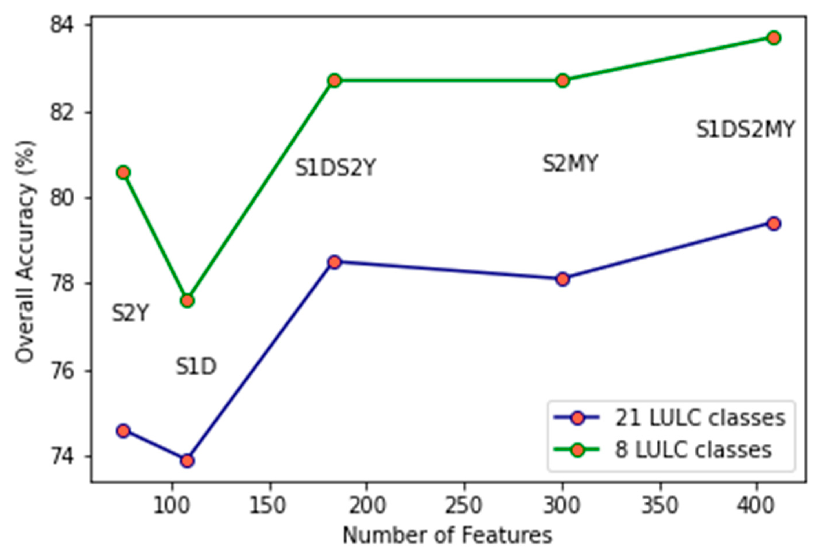
| Feature Set | Abbreviation | Number of Training Samples | Number of Validating Samples | Number of Features | OA (21 Classes) | OA (8 Classes) |
|---|---|---|---|---|---|---|
| S1 Decadal + S2 Monthly and Yearly features | S1DS2MY | 1,749,604 | 81,448 | 408 | 79.4% | 83.7% |
| S1 Decadal + S2 Yearly features | S1DS2Y | 1,950,922 | 81,448 | 183 | 78.3% | 82.7% |
| S2 Monthly and Yearly features | S2MY | 1,749,614 | 81,448 | 300 | 78.1% | 82.7% |
| S2 Yearly features | S2Y | 1,950,932 | 81,448 | 75 | 74.4% | 80.5% |
| S1 Decadal features | S1D | 1,950,922 | 81,448 | 108 | 73.9% | 77.6% |
| Comprehensive Class | Code | 210 | 220 | 230 | 240 | 250 | 290 | 300 | 500 | Total | UA | F1-Score |
|---|---|---|---|---|---|---|---|---|---|---|---|---|
| Cereals | 210 | 13,391 | 188 | 360 | 227 | 334 | 958 | 42 | 925 | 16,425 | 81.5% | 83.0% |
| Root crops | 220 | 18 | 834 | 20 | 33 | 1 | 9 | 0 | 6 | 921 | 90.6% | 80.4% |
| Non-permanent industrial crops | 230 | 45 | 29 | 2042 | 55 | 13 | 137 | 3 | 92 | 2416 | 84.5% | 79.7% |
| Dry pulses, vegetables and flowers | 240 | 18 | 34 | 25 | 193 | 19 | 53 | 2 | 34 | 378 | 51.1% | 35.1% |
| Fodder crops | 250 | 7 | 0 | 0 | 6 | 178 | 1 | 0 | 15 | 207 | 86.0% | 15.7% |
| Bare arable land | 290 | 28 | 8 | 18 | 16 | 2 | 612 | 11 | 141 | 836 | 73.2% | 39.5% |
| Woodland and Shrubland | 300 | 530 | 22 | 79 | 43 | 113 | 217 | 30,473 | 4027 | 35,504 | 85.8% | 90.5% |
| Grassland | 500 | 1818 | 38 | 163 | 150 | 1398 | 274 | 1293 | 19,627 | 24,761 | 79.3% | 79.1% |
| Total | 15,855 | 1153 | 2707 | 723 | 2058 | 2261 | 31,824 | 24,867 | 81,448 | OA = 82.7% | ||
| PA | 84.5% | 72.3% | 75.4% | 26.7% | 8.6% | 27.1% | 95.8% | 78.9% | ||||
Publisher’s Note: MDPI stays neutral with regard to jurisdictional claims in published maps and institutional affiliations. |
© 2022 by the authors. Licensee MDPI, Basel, Switzerland. This article is an open access article distributed under the terms and conditions of the Creative Commons Attribution (CC BY) license (https://creativecommons.org/licenses/by/4.0/).
Share and Cite
Ghassemi, B.; Immitzer, M.; Atzberger, C.; Vuolo, F. Evaluation of Accuracy Enhancement in European-Wide Crop Type Mapping by Combining Optical and Microwave Time Series. Land 2022, 11, 1397. https://doi.org/10.3390/land11091397
Ghassemi B, Immitzer M, Atzberger C, Vuolo F. Evaluation of Accuracy Enhancement in European-Wide Crop Type Mapping by Combining Optical and Microwave Time Series. Land. 2022; 11(9):1397. https://doi.org/10.3390/land11091397
Chicago/Turabian StyleGhassemi, Babak, Markus Immitzer, Clement Atzberger, and Francesco Vuolo. 2022. "Evaluation of Accuracy Enhancement in European-Wide Crop Type Mapping by Combining Optical and Microwave Time Series" Land 11, no. 9: 1397. https://doi.org/10.3390/land11091397
APA StyleGhassemi, B., Immitzer, M., Atzberger, C., & Vuolo, F. (2022). Evaluation of Accuracy Enhancement in European-Wide Crop Type Mapping by Combining Optical and Microwave Time Series. Land, 11(9), 1397. https://doi.org/10.3390/land11091397