Distribution and Structure Analysis of Mountain Permafrost Landscape in Orulgan Ridge (Northeast Siberia) Using Google Earth Engine

Abstract

An analysis of the landscape spatial structure and diversity in the mountain ranges of Northeast Siberia is essential to assess how tundra and boreal landscapes may respond to climate change and anthropogenic impacts in the vast mountainous permafrost of the Arctic regions. In addition, a precise landscape map is required for knowledge-based territorial planning and management. In this article, we aimed to explore and enhanced methods to analyse and map the permafrost landscape in Orulgan Ridge. The Google Earth Engine cloud platform was used to generate vegetation cover maps based on multi-fusion classification of Sentinel 2 MSI and Landsat 8 OLI time series data. Phenological features based on the monthly median values of time series Normalized Difference Vegetation Index (NDVI), Green Normalized Difference Vegetation Index (GNDVI), and Normalized Difference Moisture Index (NDMI) were used to recognize geobotanical units according to the hierarchical concept of permafrost landscapes by the Support Vector Machine (SVM) classifier. In addition, geomorphological variables of megarelief (mountains and river valleys) were identified using the GIS-based terrain analysis and landform classification of the ASTER GDEM scenes mosaic. The resulting environmental variables made it possible to categorize nine classes of mountain permafrost landscapes. The result obtained was compared with previous permafrost landscape maps, which revealed a significant difference in distribution and spatial structure of intrazonal valleys and mountain tundra landscapes. Analysis of the landscape structure revealed a significant distribution of classes of mountain Larix-sparse forests and tundra. Landscape diversity was described by six longitudinal and latitudinal landscape hypsometric profiles. River valleys allow boreal–taiga landscapes to move up to high-mountainous regions. The features of the landscape structure and diversity of the ridge are noted, which, along with the specific spatial organization of vegetation and relief, can be of key importance for environmental monitoring and the study of regional variability of climatic changes.

1. Introduction

Permafrost landscapes of mountainous areas and the plains are fundamentally different. The diversity and uniqueness of mountain landscapes are determined by the altitudinal environmental gradient [1]. The mountainous regions of Northeast Siberia have a complex topography with an altitude range of about 2000 m, underlain by continuous permafrost. These conditions determine the environmental gradient, which contains variations of the boreal forest and the arctic tundra landscapes. Such mountain ecosystems are identified as highly vulnerable to climate changes and human impact [2]. An increase of ground temperature leads to a change in the current processes in the landscape function and environmental cycles (hydrothermal, biogeochemical, and other) [3]. Carbon emissions by permafrost thawing produce positive feedback and contribute to an increase in temperature and aridity. That condition increases the risk of catastrophic forest fires, landslides, glacier melting, and permafrost degradation in the boreal forests and arctic tundra [4,5], as well as forest expansion and tundra “greening” [6]. The impacts of these processes and their consequences are still not well known, mainly due to the lack of long-term monitoring in these territories, including meteorological observations, a poor understanding of the landscape structure and a lack of spatial data on the environmental parameters [7]. Mapping based on remote sensing data is almost the only available method for the study of structural, dynamic, and spatial characteristics of mountain permafrost landscapes in this part of the world [8].

Determination of the spatial structure and landscape diversity through mapping is due to the widespread use of landscape information in matters of environmental management and strategic planning of the territorial development in the Arctic regions. The relevance of this activity is also increasing in the new context of ensuring human security and contributing to the achievement of the Sustainable Development Goals in terms of climate action, the threat to biodiversity, and increasing of the environmental risks [9]. Furthermore, the landscape maps are broadly used in the management of land, water, and forest resources, law, and urban planning [10,11,12].

For these purposes, a holistic approach of geosystemic and morphological landscape concepts is used, which defines a landscape as a model organized by a spatio-temporal combination of environmental components and landscapes of a lower hierarchical rank. These environmental components can be categorized into lithogenic, hydrogenic, climatogenic, biogenic, and anthropogenic ones [13]. The landscape maps are developed by determination of spatial configuration of these components in the form of environmental variables in accordance with available geospatial data and knowledge. These landscape concepts are used for the hierarchical classification by applying the holistic approach [14]. In general, each region of the world has adopted different landscape typology, depending on regional or local characteristics of ecosystems, landscape concepts, and taxonomic organization approaches, or adapted to the needs of land management. On the territory of Yakutia (Eastern Siberia), the concept of permafrost landscapes has long been used in a system with a heuristic structure, divided into horizontal and vertical subsystems according to certain distinctive features inherent in its components [15,16]. One of the unique features of these landscapes is the presence of permafrost, which is reflected in the typology. As for territories located in the permafrost zone (of cryolithozone), the development and dynamics of landscapes are largely determined by the properties of permafrost as a leading element of the lithogenic component (distribution, ground temperature, active layer, cryogenic process). Therefore, the definition and concept of permafrost landscapes was used for this study [17].

The classification of permafrost landscapes has changed and is being supplemented in recent decades. The impetus for this change and modernization is the development of technological capabilities for obtaining geospatial data, their processing, analysis, and interpretation. GIS-based analysis, remote sensing and, nowadays, big data processing and cloud platforms are driving new possibilities in mapping, typology of permafrost landscapes, and analysis of ecosystem changes [5,6]. The adopted typology of permafrost landscapes is associated with many relevant studies separately on the geology of landscape components, hydrography, biogeographic modeling, and environmental risk assessment [18,19]. The concept of landscapes described in the recent research are determinated by the remote sensing and GIS modeling for the identification of the geospatial landscape units [20,21,22,23]. These approaches create a unified common concept of the earth’s surface, expressed in a hierarchical classification of landscapes based on the similarity of ecological processes, patterns of distribution, and location.

In our research and according to the permafrost landscape concept, we used the Landsat 8 OLI and Sentinel 2 MSI remote sensing data and combined machine learning and GIS-based analysis for mountain permafrost landscapes mapping of the Orulgan Ridge in Northeast Siberia.

2. Background

There are many studies in the field of landscape structure, change, and dynamics based on the modeling of remote sensing data and GIS-based analysis [13,16,22]. The issues of improving the methods of mapping and modeling remote sensing data are mainly aimed at the accuracy and efficiency of determining the landscape structure and land cover change [24]. The Earth observation data used became multisensory (sensors of the Landsat, Sentinel, WorldView, MODIS series, etc.) [25,26]. Time series analysis by the application of artificial intelligence (machine learning and deep learning algorithms) allowed landscape mapping in order to identify the parameters of climate change, permafrost, and land degradation, as well as land use management. For example, Belgiu and Csillik [27] applied object-based and pixel-based classifications using phenological patterns and a time series of Sentinel 2 images to map the croplands. The patterns of the dynamics of biomass were used for recognizing the arable land in a series of MODIS and Landsat images in savannah landscape [28].

Cloud calculator platforms such as Google Earth Engine (GEE) are becoming the main tools for landscape modeling research at the regional scale. For example, Liu et al., [5] analyzed the greenness trend over the arctic tundra in Russian Federation using all available dataset Landsat archives from 1984 to 2018 in the catalog of GEE. Using the Sentinel 2 dataset on the GEE platform, the distribution of Spartina alterniflora along the coast of Southern China was mapped [29,30]. Based on the PVI and NDVI, the authors proposed supervised and unsupervised classification methods for determining the threshold values of the indices for the recognition of plant species. The platform is actively used for monitoring and mapping the forest landscapes [31] and agriculture [32]. DeLancey et al. [33] used Sentinel 2 data and SRTM topographic data for the classification of peatlands and wetlands with high overall accuracy in the Boreal Forest Natural Region, Canada. This example also presents the possibilities of data synthesis of optical satellite images and digital elevation models (DEM) for landscape objects recognition. DEM and derived datasets (slope, aspect, ruggedness, topographic indices, river basin, and shady relief) have been used by researchers for geomorphological and geomorphometric landscape studies [14]. In fact, landforms such as uplands, slopes, terraces, and valleys have strong links with lithology and geomorphology, which make them good variables for landscape identification in different scales. Additionally, machine learning classification by the topographical attributes is used for digital soil mapping and spatial distribution patterns of soil nutrients [34].

The application of GIS and remote sensing in the study of the permafrost landscape is widely represented both in mapping on the local scale and in general maps at the regional scale such as in the Permafrost landscape map of the Republic of Sakha (Yakutia) [6]. However, most of the research is directed towards identifying the landscapes changes, for example, Jorgenson et al. [35] determined the dynamics of ecosystems of the river delta and coastal areas in the Yukon-Kuskokwim Delta through a time series of satellite images and aerial imagery. The authors presented an extensive classification of ecotypes with the identification of 29 ecosystem types and provided with environmental description. Many studies have been presented in special issues of “Geosciences” and “Land” in the last years [36,37].

In our previous studies, we used time-series Landsat 8 data of 2019–2020 to define six types of permafrost landscapes in the Adycha-Elga plateau, Northeast Siberia to compile a permafrost landscape map at scale of 1:200,000 [38]. For this, we developed a method for the classification of vegetation cover by the photosynthetic activity using vegetation indices and landforms made by GIS-based terrain analysis for the determination of permafrost landscapes types [39]. The development of cloud calculators for processing big remote sensing data gave us the opportunity to expand the research and adapt the methodology on a regional scale mapping of mountain permafrost landscapes.

3. Methodology and Materials

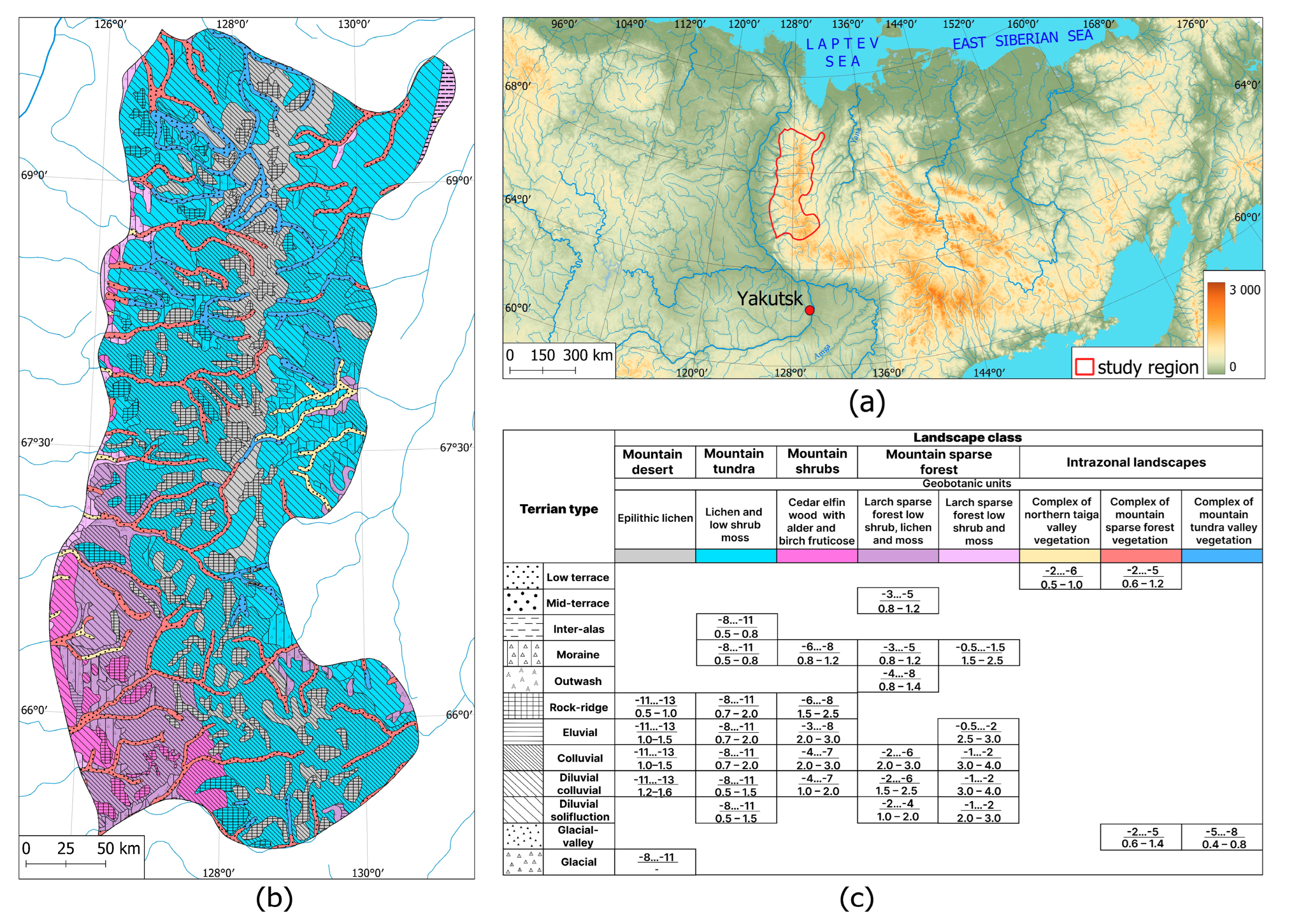
3.1. Study Region

The study region is the Orulgan ridge, belonging to the western highest part of the Verkhoyansk Mountains. The territory of the ridge is determined by the zoning of permafrost-landscape regions (provinces) [15]. The Orulgan Ridge in Figure 1a is characterized by a meridional orographic structure and the presence of all varieties of mountain permafrost landscapes in the Arctic territories, which makes it a reasonable choice among the other mountain regions in terms of coverage and diversity.

The entire region is a territory of traditional land use of Evens, the indigenous people of Arctic Siberia. Their economic activities are reindeer herding, hunting, and fishing. Reindeer herds roam the mountain tundra and mountain river valleys [40]. The most elevated central part of the ridge is under protection in the status of a resource reserve (habitat area for bighorn sheep). Geological surveys confirm the presence of large deposits of mineral resources; strategically, the region has prospects for the development of gold, silver, lead, and tin mining industry [41].

According to Fedorov et al. [15], the study region is characterized by a mid-altitude mountain permafrost landscape province with an elevation of 2224 a.s.l. The ridge (landscape province) is located in the continuous permafrost zone with a predominance of mountain-tundra and mountain-sparse forest or woodland permafrost landscapes. In the river valleys, the boreal taiga permafrost landscapes by Larix, Populus, and Salix are recognized. It spreads to the north and higher elevations, regardless of the climatic zone of distribution [25,42]. The geomorphological and lithogenic compositions are dominated by slope colluvial and deluvial colluvial terrain types, as well as accumulative moraine and outwash flat slopes. In total, according to the map of permafrost landscapes of the Republic of Sakha (Yakutia), the study region Figure 1b has 5 classes of permafrost landscapes with 9 vegetation units and 12 terrain types [17]. Permafrost parameters are determined by configurations of vegetation (geobotanical) units and terrain types, which are shown in Figure 1c. Permafrost varies greatly depending on the landscape class and lithological and geomorphological characteristics of terrain types. Our study was focused on vegetation (identification of geobotanical units), since our previous studies showed that in mountainous areas, terrain types have high contrast and fragmentation, which is why the visual representation of the map is very difficult and does not meet the goals of regional mapping in terms of distribution [38,43]. For the regional level of mapping, we did not implement the use of DEM analysis to identify all types of terrain, and we believe that it is necessary to map terrain types at the local level of mapping permafrost landscapes in combination with landscape types.

3.2. Permafrost Landscape Mapping Approach

There are many classification approaches to landscape mapping. We adopted the classification developed for permafrost landscape mapping [13] of the region as part of geocryological and environmental research since 1970s at the Permafrost Institute in Yakutsk. Recent studies have adopted the landscape recognition criteria for the application of GIS tools [17,26]. The classification units being mapped should be adequate for the coverage and scale of the map, which in turn depends on the spatial resolution of satellite images. The use of Sentinel 2 and Landsat 8 images with spatial resolutions of 10 and 30 m, respectively, prompts us to choose working scales in the range from 1:500,000 to 1:1,000,000. The classification of permafrost landscapes of this scale has a vertical scheme: landscapes—Terrain (mestnost)—Uroshiche (part of terrain that is different by vegetation) [13]. For reduction and landscape unity, we renamed this category to the class of landscape—Type of terrian—Type of landscape, which is presented in

Table 1. Environmental variables—Indicators of landscape classification categories [13].

Classification Categories	Geobotanical Units	Landforms	Lythology	Approximate Coverage, km2
Class of landscape	combination of vegetation associations and formations	megarelief	-	>500
Type of terrian	-	mezorelief	Quaternary deposits	50–500
Type of landscape	group of vegetation associations	mezorelief	Quaternary deposits	<50

, where configurations of environmental variables for mapping are indicated.

In our previous paper [38], we presented the results of mapping permafrost landscapes at the level of type landscape and terrain in the same Verkhoyansk mountain system. In this manuscript, we focused on the landscape classes within the entire region. The methodology for mapping permafrost landscapes consists of integrated GIS modeling, consisting of separate parts for identifying environmental characteristics—Variables. The principal environmental variables of permafrost landscapes modeling are geobotanical units (vegetation associations and formations) and the landforms (megarelief). The additional variables are the Quaternary deposits (genetic type of sediments) largely determined by the combination of principal environmental characteristics. Thus, the initial data should attempt to obtain spatial data reflecting the mentioned variables.

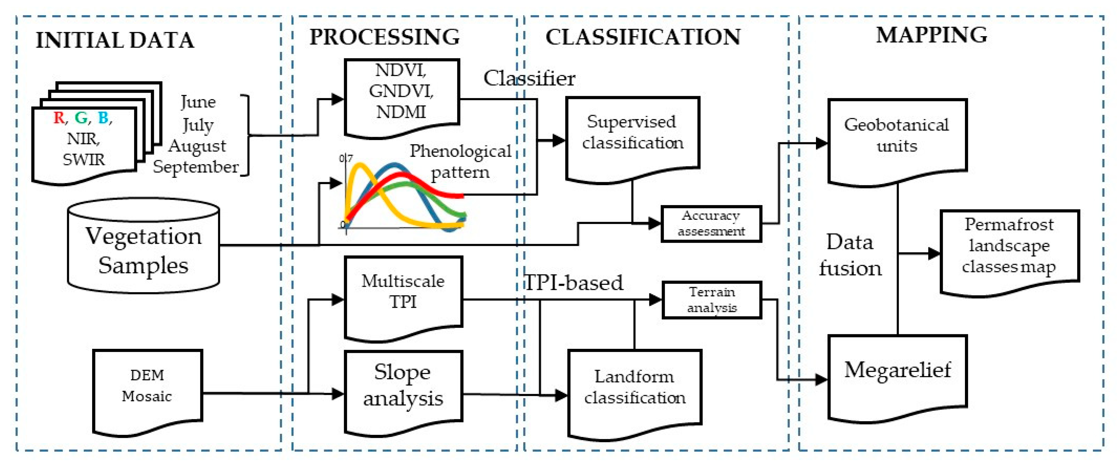
3.3. Methodology Workflow

The methodology workflow for obtaining data on the landscape structure consists of the sequential compilation and synthesis of land cover, but in this case, vegetation cover classification was performed by using the time series of Sentinel 2 MSI and Landsat 8 OLI images for the phenology-based image classification. The vegetation cover classification takes up most of the processing procedure. Since the study region covers 81,956 km², a large amount of data were used for image classification, which was successfully implemented in GEE. The GEE was created to optimize the analysis of geospatial data and can handle petabytes of remote sensing data over large geographic scales and long-time coverage [42]. The GEE has a database of pre-processed Sentinel 2 MSI and Landsat 8 OLI images (Top of Atmoshpere and surface reflectance) and a wide range of integrated machine learning algorithms for supervised classification. Landform classification was performed by the GIS-based terrain analysis (river valleys and positions in the mountains) by the ASTER GDEM scenes data. The characteristics of the relief and the genetic sediments were compiled in terrain analysis of morphomethic variables—slope and topographic position. The general scheme of the methodological approach is illustrated in Figure 2.

Then, we considered the implementation of each stage of the methodology working flow, finally leading to the production of two spatial layers of environmental variables of permafrost landscapes. These two spatial layers were combined to obtain landscape classes of valley and mountain ecosystems.

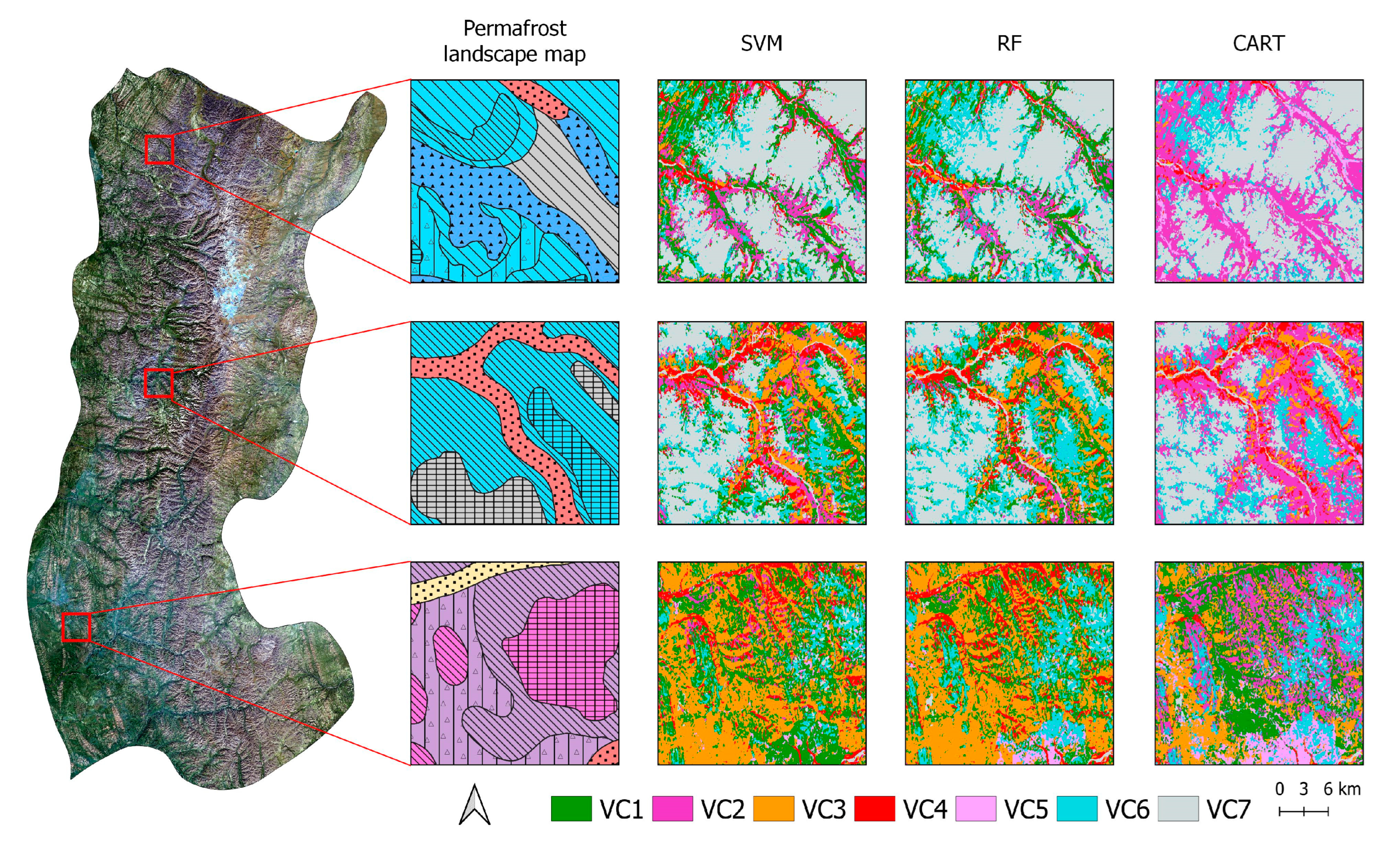
3.4. Vegetation Cover Classification

The objective of image classification is to discriminate geobotanical units as an indicator of landscape classification. Vegetation associations and formation are not the typical objects of image classification in remote sensing. The selection of the vegetation associations is carried out according to the principles of dominance plants approach in geobotanical classification [44]. Associations are classified primarily on the basis of species composition and diagnostic species (i.e., plant species by which we can discriminate them from others). Combination of the vegetation associations, or “alliance” in some sources [45,46], is a unit of vegetation cover classification containing one or more associations with a characteristic range of species composition, environmental conditions, physiognomy, and diagnostic species, usually at least one of which is located in the uppermost or dominant layer of vegetation. At the regional level, we refer to the fact that the combinations of vegetation associations differ in seasonal photosynthetic activity for Northeast Siberia by the period from June to September. The study region in high mountain areas with poor biodiversity can even be covered with vegetation formations (epilitic lichens). Therefore, in this study, for the identified classes of modeling based on remote sensing data, we defined them as mapped geobotanical units [39]. For this aim, a phenology-based classification approach was applied. GEE Image Collections were selected based on cloud-free filter images separately for periods (mid-June, July, August, and early September). Sentinel-2 images launched by the Copernicus program of the European Space Agency (we used 5 bands: Blue 490 nm, Green 560 nm, Red 665 nm, near infrared (NIR) 842 nm and short wave infrared (SWIR) 1610 nm at 10 m spatial resolution) and Landsat 8 OLI images launched by NASA and United States Geological Survey (we used 5 bands: Blue 483 nm, Green 560 nm, Red 660 nm, NIR 865 nm and SWIR 1620 nm at 30 m spatial resolution) were used. The size of the study area is covered by 15 full Sentinel 2 imagery scenes and 7 Landsat 8 scenes. For the entire study area there were 550 images of Sentinel 2 extracted in total for the period 2015–2020 and 223 images of Landsat 8 OLI images for the period 2013–2020 (see

Table 2. Landsat 8 OlI and Sentinel 2 dataset of the study region in GEE.

Date	Sentinel 2 All Data	Landsat 8 OLI All Data	Sentinel 2 Cloud-Free Data	Landsat 8 OLI Cloud-Free Data
Early September	610	293	124	48
August	909	423	138	68
July	921	368	210	75
Late June	448	165	78	32
Total	2888	1249	550	223

).

Single red, green, and blue NIR and short wave infrared (SWIR) spectral bands are useful for identifying vegetation state and phenological phase in color composite. For each collection of images, we calculated the vegetation indices: the widely used NDVI in Equation (1), GNDVI in Equation (2), and NDMI in Equation (3). Subsequently, we created monthly vegetation indices mosaics by calculating the median value for all available scenes over a specified time period over the non-snow cover months. NDVI is the general spectral index reflecting the state of plants and the volume of biomass. GNDVI is the modified vegetation index, often used in vegetation with low chlorophylls and water deficit/express, which should work well in biomass-poor areas of tundra and mountain woodlands [47]. NDMI is used to determine vegetation water content and differentiates well wetlands in river valleys and tundra swamps [48].

$$\mathrm{NDVI}=\frac{NIR-RED}{NIR+RED}$$

(1)

$$\mathrm{GNDVI}=\frac{NIR-GREEN}{NIR+GREEN}$$

(2)

$$\mathrm{NDMI}=\frac{NIR-SWIR}{NIR+SWIR}$$

(3)

The vegetation cover is characterized, generally, by the absence of evergreen tree species and the predominance of sparse Larix forests. The class of sparse forests was differentiated depending on the composition of the lower layers (shrubs and lichen or low shrub-herb cover) [49]. The lower vegetation layer has a significant impact on the spectral characteristics of satellite images. Differences in the values of the spectral indices make it possible to separate the low shrub-lichen tundra from the epilithic-lichen cover. Valley forests and sparse Larix forests with Siberian low pine in the mountain slopes have almost the same spectral values throughout the summer, but valley forests, due to the presence of alder, poplar and willow, lose their biomass very rapidly by the beginning of September. These phenological features allow us to distinguish them from each other. The river valley areas are distinguished by high biodiversity and heterogeneous composition of the vegetation associations. In addition, the mountain river valleys represent water streams on pebble alluvium, the spectral characteristics of which are close to epilithic lichens. This division leads to spatial mosaicism, which does not correspond to the scale of the study. Therefore, the vegetation of the northern taiga valleys is composed of combinations of willow-alder communities with areas of larch, poplar, and chozenia forests.

Training and validation samples of vegetation classes require a geobotanical analysis of the study region. The collected biogeographical data of field surveys in the region and the Verkhoyansk Range as a whole allowed us to analyze high-resolution images. Field surveys were conducted in July and August 2018–2019 on the eastern slope of the Orulgan Ridge, and also identified visual interpretations using very high-resolution images in Google Earth Planet and Yandex Sattelite based on field materials and geobotanical data from early studies at this region with geobotanic or floric descriptions [50,51] and the resulting maps [52]. The method of expert determination of training data is often used in studies of vegetation types and cover [31,53]. A total of 326 samples were selected for training and 735 for validation. The regional scale of mapping and reference to the classification of permafrost landscapes allowed us to identify 7 geobotanical units of vegetation cover (VC) (see

Table 3. Geobotanical units and sample data.

Code	Geobotanical Units	Training Samples	Validation Samples
VC1	Larix sparse forests with low shrubs, lichen and green moss	58	95
VC2	Larix sparse forests with lichen and green moss	34	90
VC3	Larix sparse forests with low shrub—Lichen and Pinus pumila in combination with Duschekia fruticosa shrubs	56	85
VC4	Alder and willows with areas of Larix, Populus and Chozenia forest	65	115
VC5	Larix sparse forest with bogs	56	120
VC6	Lichen and low shrub	23	120
VC7	Epilithic lichens and non-vegetation cover	34	110
	Total	326	735

).

To achieve the best image classification result, we used three machine learning algorithms integrated in GEE: Support Vector Machine (SVM) [54], Random Forest (RF), and Classification and Regression Tree (CART). Figure 3 shows the results of the classification, where SVM and RF had close results; on the contrary, CART strongly absorbed some vegetation classes. To compare the results, we calculated the confusion matrix of classifications, according to which the producer accuracy (PA), user accuracy (UA), overall accuracy (OA), and Kappa coefficient were calculated to determine the effectiveness of the algorithms [55].

Table 4. Classification accuracy of three classifiers.

Vegetation Classes	SVM		RF		CART
	PA, %	UA, %	PA, %	UA, %	PA, %	UA, %
VC1	90	88	77	82	67	78
VC2	88	83	87	82	74	83
VC3	85	82	79	79	68	77
VC4	83	85	82	78	77	55
VC5	88	88	82	84	73	74
VC6	74	76	70	71	68	68
VC7	79	84	76	79	79	61
Overall accuracy, %	85.4		78.5		70.8
Kappa coefficient	0.74		0.61		0.47

shows the accuracy of the classification results obtained using the three classifiers. OA and kappa by SVM were 85.7% and 0.74, respectively. While the RF classification accuracy was acceptable, the PA and UA of some vegetation classes were not high. For RF, stumpy results were recorded in the class of tundra vegetation (VC6) and shrub vegetation (VC3). For CART, a high proportion of confusion was found in forest vegetation (VC1), valley vegetation (VC4), and tundra (VC6). CART greatly reduced the proportion of VC1 due to tundra and shrub vegetation (VC3).

Thus, for landscape mapping, we determined the SVM according to an acceptable result of vegetation classification. SVM is a supervised non-parametric statistical learning algorithm, which has made it possible to achieve effective classification results in various remote sensing studies, including vegetation mapping according to NDVI [56] and landscapes mapping of heterogeneous areas [29]. We configured SVM with a radial basis function as the kernel type, a moderate cost-parameter value 15, and a Gamma term equal to 0.2. The result obtained had the effect of “salt and pepper”—small areas of class values in terms of the number of pixels. To remove such noise after export from the cloud platform, we used the “Sieve” tool in the QGIS with a threshold of 500 m, respectively to the coverage. The tool removes pixels smaller than the specified threshold size and replaces them with the pixel value of the largest adjacent pixel.

The most accurately classified geobotanical unit VC1 is Larix sparse forests with low shrubs, lichen, and green moss. Most of the incorrectly classified pixels were assigned to the mountain tundra and desert classes VC6 (Lichen and low shrub) and VC7 (Epilithic lichens and non-vegetation cover). Confusions of VC7 are also due to the fact that incompatible geobotanical units are merged in it, such as river gravel, water, and epilithic lichens of high mountain areas. This lack of spectral image classification requires the use of other differentiation methods, such as terrain analysis.

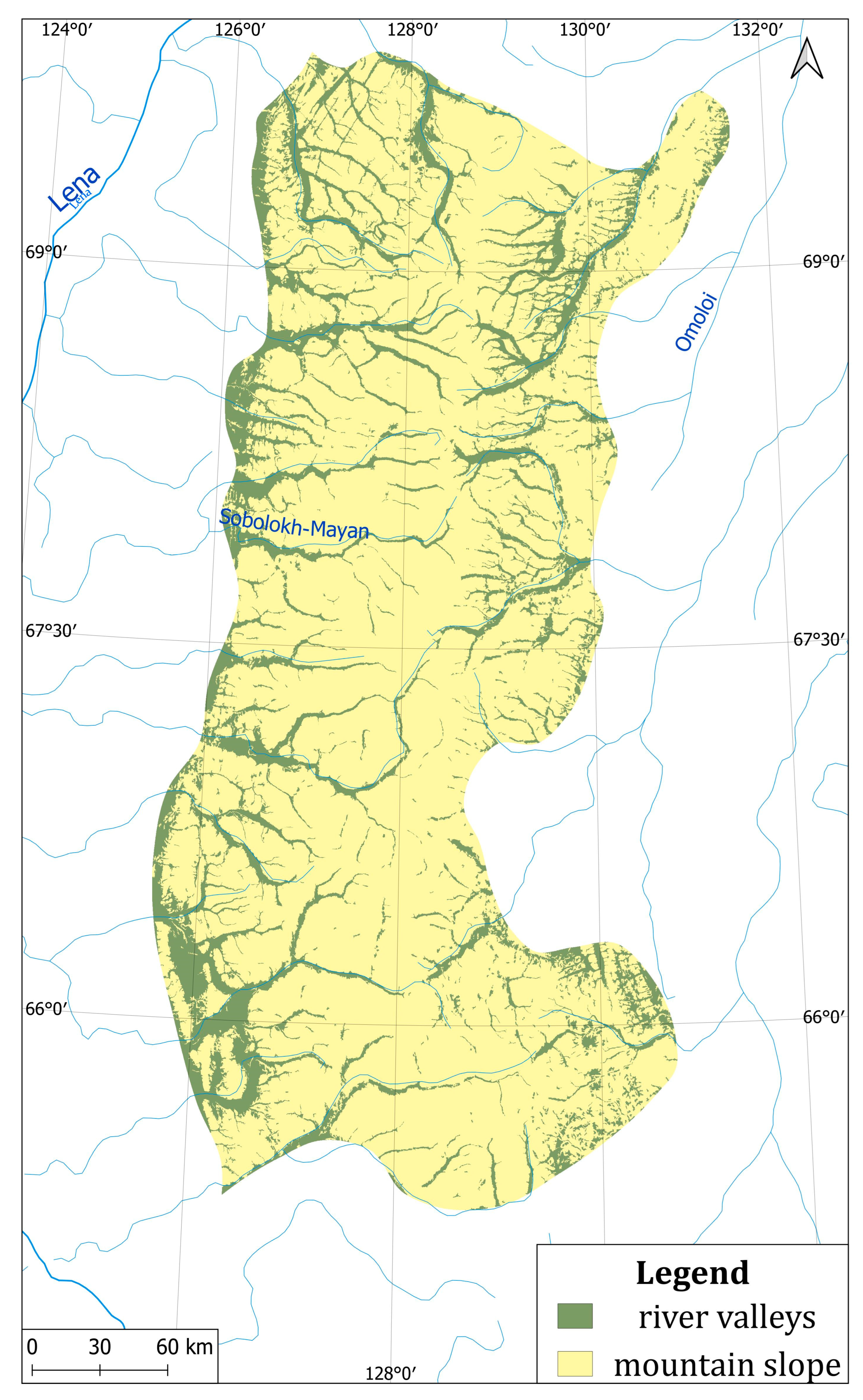
3.5. GIS Terrain Analysis

Terrain analysis is used to determine two groups of classes of permafrost landscapes: zonal and intrazonal. In the structure of mountain landscapes, as nowhere else, the main regularities of geographical distribution of climate conditions (altitudinal temperature gradient, latitudinal climate zoning, and sectorial longitude separation) are manifested. As an environmental variable of the permafrost landscapes differentiation, relief increases its significance with the detailed classification of landscapes (at the level of group and types of landscape). Intrazonality is determined by the presence of landscapes atypical for the latitudinal zone under the influence of local climatic and hydrological factors, mainly formed in river valleys [57]. The river valleys form intrazonal landscapes; therefore, the analysis of the terrain according to DEM is necessary to distinguish two types of megarelief—valleys and mountains.

We already used the method of landform classification at the local level with the topographic position index (TPI) [58]. The slope degree and TPI [59] was used to perform landform classification from improved version 3 of Advanced Spaceborne Thermal Emission and Reflection Radiometer (ASTER) Global DEM with 30 m spatial resolution. In total, the study region covers a mosaic of 22 clipped scenes. The resulting mosaic of scenes had a number of anomalous values that were eliminated using the DTM filter tool in SAGA GIS. The artifacts were assigned a null value, then the contours were created with a step of 15 m, and the values were interpolated. In addition, with the help of bilinear interpolation and slope-based filtering, we removed adjacent cells with a large difference in elevation, which could hardly be caused by real terrain conditions. The filter determines the allowable height difference between two cells as a function of the distance between cells [60]. The procedure is performed in two steps in SAGA GIS and GRASS GIS. The result of DEM preprocessing is presented in Figure 4.

The TPI algorithm in Equation (4) compares the elevation (E) of each cell in a DEM to the mean elevation (Em) of a specific neighborhood around the cell (n—number of cells), thus revealing the position of the cell relative to neighboring ones. Unsupervised classification by Jenness [58] was implemented on the basis of two sizes of radius (scale): large 2500 m and small 300 m. Gaussian weighting was used with a bandwidth value of 50. TPI-based landform classification released in SAGA GIS [60].

$$TPI=E-{\displaystyle \sum }_{n-1}Em/n$$

(4)

Ten classes of landforms were produced: streams, mid-slope drainages, local ridges, valleys, plains, foot slopes, upper slopes, upland, mid-slope ridges, and mountain tops. For the purpose of mapping classes of landscapes, we only needed to obtain two types of combined landforms, i.e., river valleys and mountains. We used a reclassification based on two processed data: analysis of slopes and landforms. River valleys included streams, valleys, plains, and foot slopes (partially), while the rest were combined as mountain slopes. The reclassification result is shown in Figure 5.

The obtained data on the megarelief let us distinguish intrazonal valley landscapes by classifying the slope with a steepness threshold of 15° into valleys and mountain slopes. This slope value is optimal as a threshold between the mountain slope and river valleys for differentiating intrazonal valley landscapes from mountain permafrost landscapes.

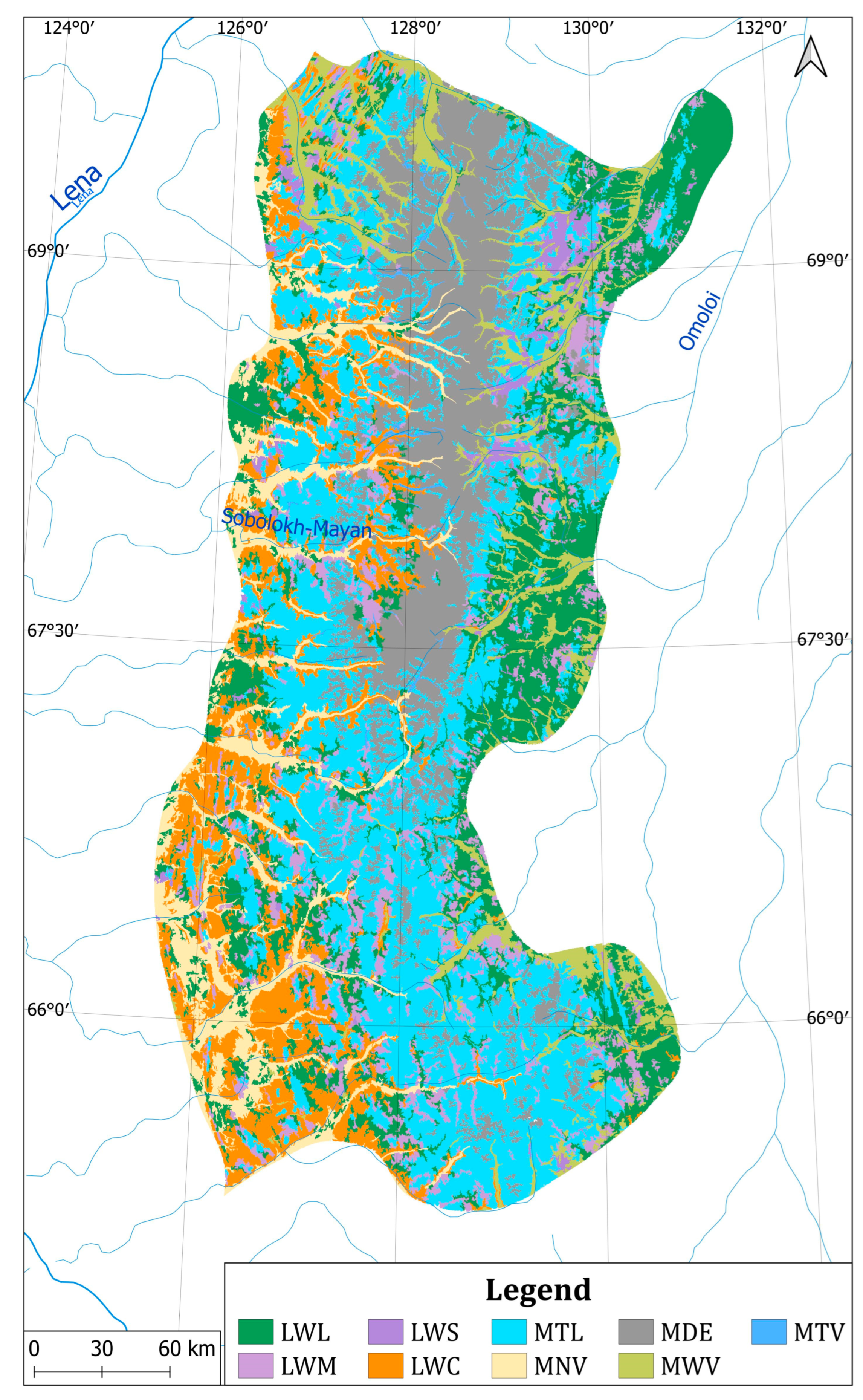
3.6. Landscape Mapping and Data Synthesis

The holistic landscape classification approach uses the landscape concept as a complex system of functions consisting of a set of variables. The variables are determined by the factors of landscape formation, the number of which differs in many studies [17,18,20,61]. Therefore, the use of a holistic representation of the landscape in this concept allowed us to restrict ourselves to the available spatial data in GIS for synthesizing and mapping classes of permafrost landscapes. The obtained data of vegetation and relief are the sought-after ways to conceptualize the landscape structure with the spatial data available to us [62] and yet it is acceptable for classification at the regional level. Spatial stacking of layers in GIS of the vegetation and types of megarelief is a method of data synthesis for mountain permafrost landscape mapping.

4. Results and Discussion

As a result, we identified nine classes of permafrost landscapes: three valley intrazonal landscape complexes and six zonal classes of mountain permafrost landscapes. The compiled permafrost landscape map of the Orulgan Ridge is presented in Figure 6 and the description of the discriminated mountain permafrost landscape is provided in

Table 5. Classification and description of permafrost landscape classes of the Orulgan Ridge.

Permafrost Landscape Class	Code	Description
Mountain desert	MDE	Landscape of the arctic deserts. Vegetation is sporadic or absent. Lichen (Rhizocarpon geographicum, Haematomma ventosum, Umbilicaria). Mountain peaks and steep mountain slopes.
Mountain tundra	MTL	Landscape of the arctic tundra. Lichens (Alectoria ochroleuca, Coelocaulon divergens), low shrubs (Dryas punctata, Cassiope tetragona). Steep near-summit slopes, mountain top surfaces, slopes of the northern or eastern exposure.
Sparse Larix forests, low shrub, lichen and moss	LWL	The most common class of Larix sparse forest landscape. They are common on gentle slopes or at the foot of steep slopes. Low shrubs are represented by Ledum palustre, Vaccinium uliginosum, V. vitis-idaea. Lichens (Cetraria cucullata) mosses (Aulacomnium turgidum).
Sparse Larix forests, lichen and moss	LWM	Mountain Larix sparse forest landscape. Shrub cover is practically absent. Lichens (Cetraria cucullata), mosses (Aulacomnium turgidum). They are common on medium slopes and elevated sections of slopes.
Sparse Larix forest, sphagnum	LWS	Mountain Larix sparse forest landscape. The low shrub cover is represented by Vaccinium uliginosum, Chamaedaphne calyculata, mosses (Aulacomnium turgidum, Sphagnum warnstorffi, Sph. balticum). Lichens (Cetraria cucullata), mosses (Aulacomnium turgidum). It is characterized by high humidity and the presence of swamps at the foot of slopes and flat areas.
Sparse Larix forests, low shrub—Lichen with Pinus pumila	LWC	Mountain Larix sparse forest and mountain shrubs landscape. The difference of the class is the presence of shrub layer: Betula exilis, Pinus pumila. Low shrubs: Ledum palustre, Vaccinium uliginosum, lichens (Cetraria cucullata, Cladina arbuscula) mosses (Aulacomnium turgidum, Sphagnum spp.). They are common on the slopes of the southern and western exposures and the slopes of the valleys of the Lena River basin.
Boreal taiga in valley	MNV	Intrazonal boreal taiga landscape along river valleys. Vegetation is represented by many formations and associations. Horsetail (Equisetum arvense) green-moss (Aulacomnium turgidum, Hylocomium splendens) and sphagnum (Sphagnum balticum, Sph. fimbriatum) in combination with willow meadows and grass bogs. Mixed forests of green moss (Aulacomnium turgidum) type in combination with yernik (Betula fruticosa), grasses (Calamagrostis neglecta, Agrostis trinii), sedge (Carex stans, C. minuta, C. atherodes) and cotton-grass (Eriophorum polystachyon). They are distributed along the valleys of the Lena River basin.
Mountain forest in valley	MWV	Intrazonal mountain sparse forest landscape along river valleys. Larix forest with Ledum palustre, Vaccinium uliginosum, V. vitis-idaea with areas of chozenia (Chosenia arbutifolia) and poplar (Populus suaveolens) forests. Most of the landscapes belong to the valleys of the Yana River basin.
Mountain tundra in valley	MTV	Intrazonal mountain tundra landscape along trough valleys. Within the mountain tundra, river valleys are not developed properly. Complex tundra communities (Ledum palustre, Arctous alpina, Koenigia tripterocarpa, Andromeda polifolia, Empetrum nigrum) with sparse shrubs of Betula nana subsp. exilis represent transition between slope and riparian vegetation.

. Using the methodology for mapping permafrost landscapes, we analyzed the spatial structure of landscape classes to determine the nature of the distribution of boreal taiga and arctic tundra landscapes in the Verkhoyansk Mountain system.

The results are interpreted in two ways: by analysis of the landscape structure to identify the areas of landscape classes and comparison with the basic permafrost–landscape map of the Republic of Sakha (Yakutia) in the scale of 1:1,500,000, since we use the same classification schema (4.1); by compilation of a general scheme of elevationaland topographic distribution of landscape classes of the Orulgan ridge, it is possible to assess the geomorphological boundaries of mountain permafrost landscapes (4.2).

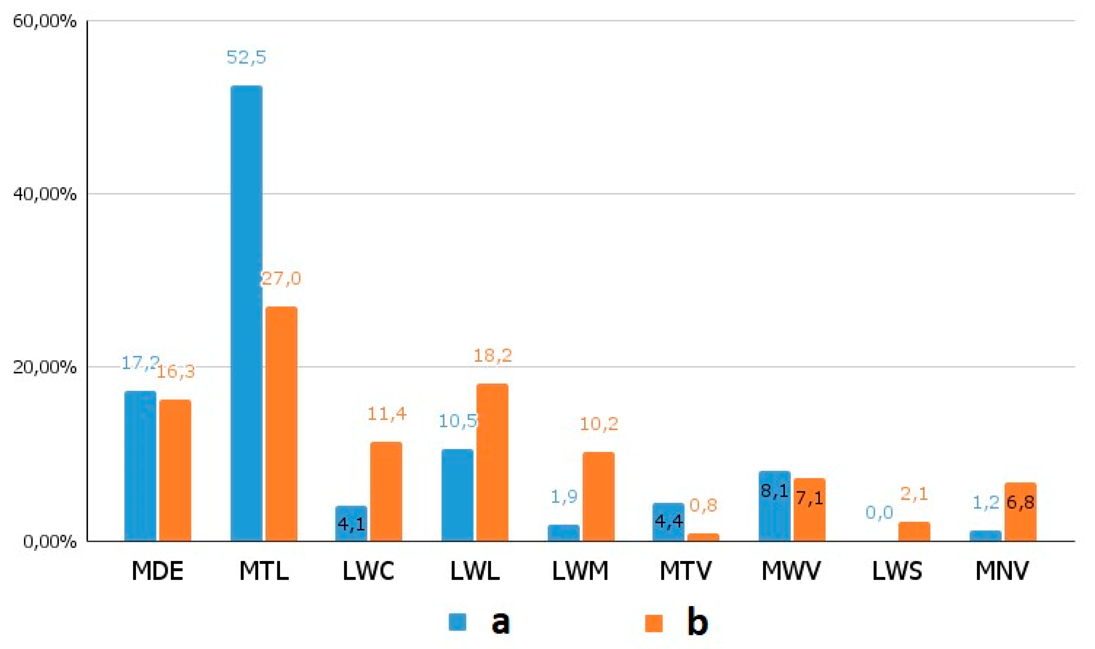
4.1. Comparison with Earlier Permafrost Landscape Mapping

Statistical analysis of the structure of landscapes made it possible to determine the degree of heterogeneity of the ridge. Figure 7 shows the areas covered by permafrost landscape classes and compares them with the equivalent classes on the Permafrost Landscape Map of the Republic of Sakha (Yakutia). If we, conditionally, combine mountain tundra and mountain desert landscapes (classes: MTL and MDE) and mountain forest and shrub landscapes (LWL, LWC, LWM and LWS), then we can notice that the ratio of arctic mountain tundra and mountain sparse forests is approximately equal to 1:1. In areal percentage terms, tundra and mountain desert occupy 27% and 16% of the territory. The most common landscape class of sparse forests occupies 18%. Such a landscape structure confirms the expediency of distinguishing a permafrost landscape region (province) as a group of mountain tundra and mountain sparse forest landscapes in the continuous permafrost zone. However, in contrast to the earlier small-scale map, we revealed significantly large areas of boreal forests and the significance of MNV and mountain Larix-sparse forest landscapes in the landscape structure of the study region, especially intrazonal landscapes in the river valleys, 1% to 7%.

A low percentage of intrazonal mountain tundra coverage is obtained because there is practically no river alluvial sediment in the glacial valleys. Therefore, at the level of landscape classes, the identification of glacial valleys is practically very difficult. The exception is some relatively gentle narrow area in small rivers. This property of glacial valleys in Verkhoyansk Mountains was distinguished by Nikolin [63]. The penetration of forests along the river valleys into the depths of the mountain range can be associated with the thermal effect of tectonic faults. Tectonic faults play a significant role in the spread of forests along river valleys as additional sources of heat from the internal energy of the Earth, which is also evidenced by numerous ice floes.

In general, the use of GIS terrain analysis and remote sensing modeling by GEE let us significantly enhance of intrazonal valleys permafrost landscapes identification. The method used distinguishes the dependence of the intrazonal landscape on the width of the transverse distribution of the valley since the width of the valley and the amount of alluvial river sediments expands along the river [1]. This aspect of river landscapes has so far been practically taken into account at the regional scale of mapping. Obtaining detailed information of the spatial structure of the valley vegetation complexes will allow further assessment of their roles in the biomass of the Arctic mountain ranges and their role in greenhouse gas emissions.

Epilithic lichen communities of stony deserts cover the tops of mountains with eluvial deposits, rock glaciers of mountain ranges, and on steep slopes, the proportion of which increases from south to north. The ridges in the southern part of the region are largely covered by mountain lichen and low shrub–moss tundra. Since the Orulgan ridge is medium-altitude, it is not covered with non-melting snow. At the same time, mountain deserts contain many slope glaciers [64]. In general, the analysis of the obtained map indicates the general latitudinal pattern of reduced share of the forest and shrub vegetations and increased areas of mountain tundra vegetation and communities of epilithic lichens and rock glaciers in the northward direction.

The difference in the area covered by tundra and boreal forest landscapes in our analysis and the published data can be associated with two aspects. Firstly, overall detail for mapping at the scale of 1:1,500,000 determines the general forms of the landscapes distribution, while our use of a semi-automatic multisensor phenology-based classification method for vegetation and terrain analysis could significantly enhance the reliability of detecting areal parameters of landscapes. The second aspect is that it can be attributed to the general trend of migration and “greening” of boreal forests, shrubs, and artic tundra due to the global warming. This phenomenon for northern latitudes has been described in many studies, for example, refs. [65,66,67]. As well as, forest fires are the leading process in the dynamics of permafrost landscapes The pyrogenic factor plays a significant role in landscape changes [68]. This issue requires further investigation to assess the sustainability of tundra and some forest classes of landscapes.

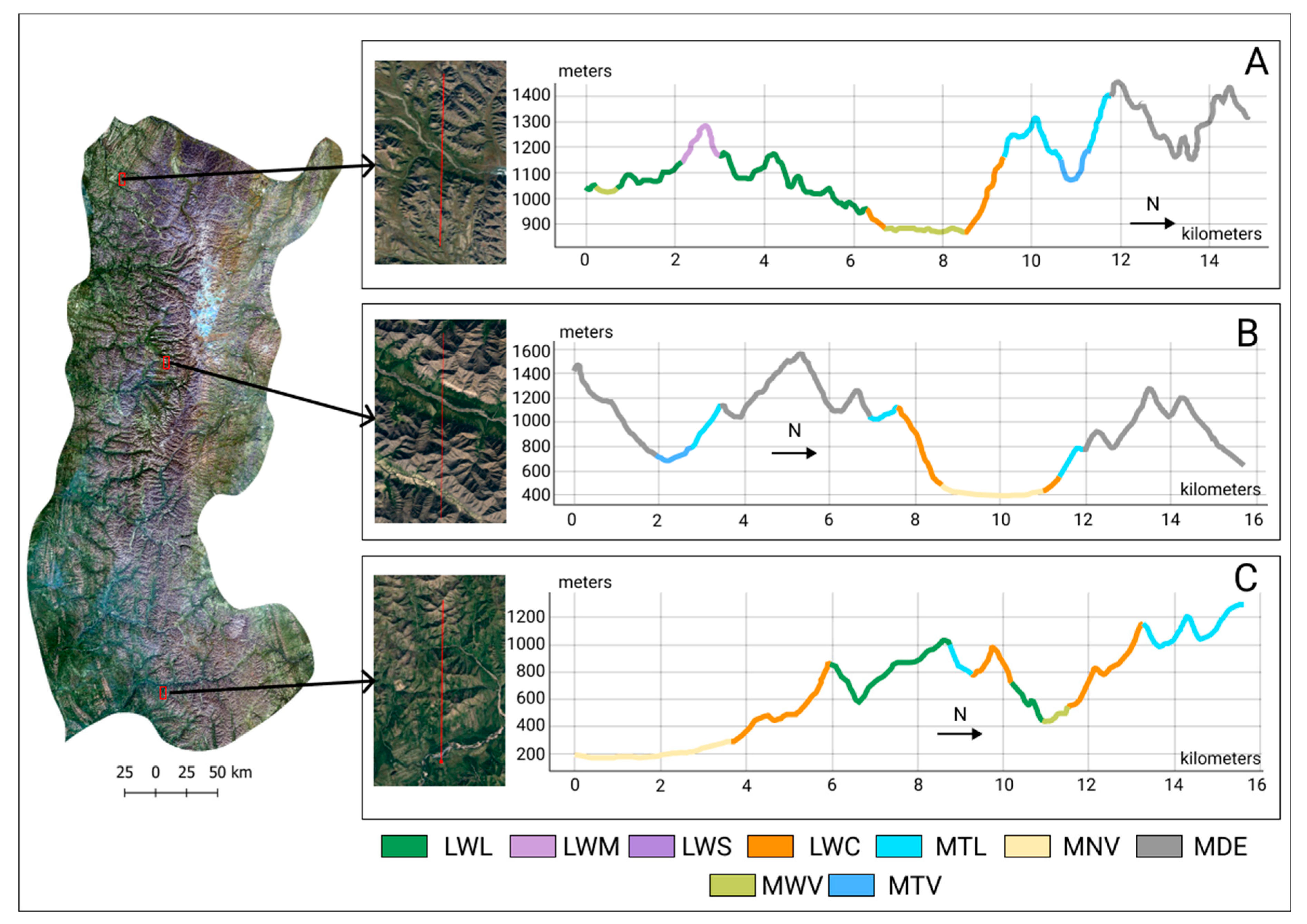
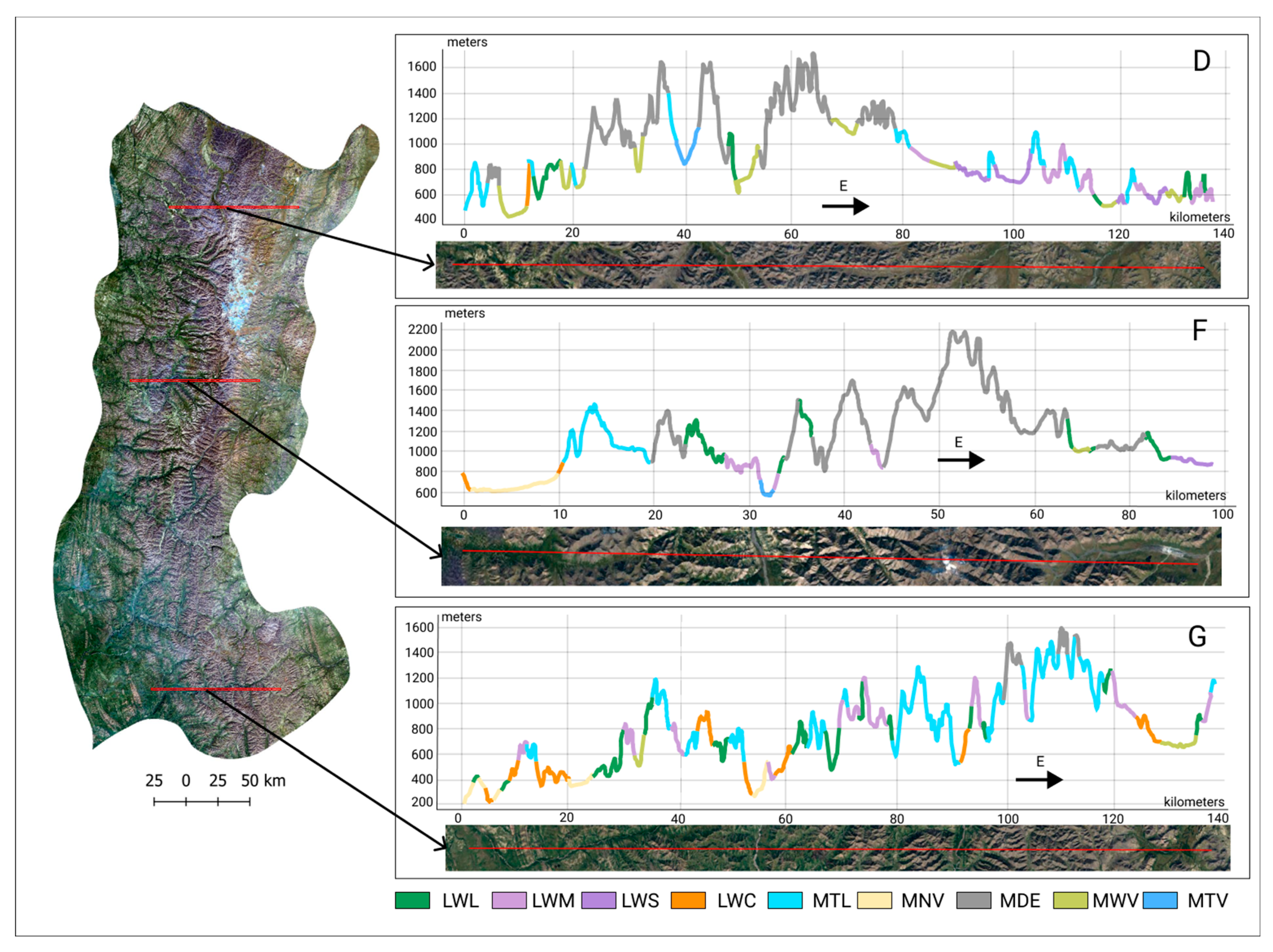
4.2. Analysis of Topographic Landscape Variability of Orulgan Ridge

The intensity of interaction and the scale of redistribution of organic matter and energy between mountain landscapes determine their topographic variability. This phenomenon is also related to the distribution of soils and the pedological term katenas. For example, Chernykh et al. [57] used macrocatenas to describe the spatial organization of the Altai Mountains landscapes. The topographic variability is largely due to the activity of exogenous agents that determine the morphogenetic types of relief, the magnitude of horizontal and vertical dissection, the energy of riverine, slope, and other processes and, accordingly, the characteristics of vegetation. To study the landscapes of the Orulgan Ridge, we plotted three longitudinal and latitudinal landscape profiles. The number and sequence of landscape classes are primarily determined by the direction and intensity of neotectonic movement. They determined the elevation of various parts of the mountain system, the layering and configuration of the megarelief elements, i.e., created the basis for the formation of the altitudinal zonation of mountain ecosystems. Thus, the relief is determined by the dissection of tectonic uplifts, erosion and transformation under the influence of cryogenic processes. On the western macroslope, there is a moraine relief inherited from the Upper Pleistocene glaciations [68].

Figure 8 shows longitudinal profiles. Profile A is made at 129°16′46″ E longitude in the northern part of the ridge with altitudes from 866 to 1459 m. Valleys are covered with MWV, and at the foot of steep slopes there is a narrow strip of LWC mountain slopes covered with LWL local peaks up to 1200 m high covered with LWM or a belt of tundra landscapes, which begins at an altitude of about 1100 m. Profile B was made in the central part of the ridge at longitude of 127°59′15.4″ E, an altitude difference from 400 m to 1555 m. Boreal forests penetrate wide river valleys. The forests on the slopes are not widespread; they occupy a narrow strip in the lower part of slopes. Narrow intrazonal MTV landscapes are formed in glacial valleys. The mountainous tundra landscape occupies steep high slopes of the southern exposure. Profile C was made in the southern part of the ridge at longitude of 126°40′48.6″ E, an altitude difference from 189 m to 1287 m. This profile clearly represents the vertical distribution of landscapes. The valley is almost 4 km wide and is covered with boreal forest with rich biodiversity. The slopes are covered with Larix forest with Pinus pumila. The flat areas of low mountains are covered with LWL. The slopes of the northern exposure are covered with mountain tundra, with a continuous tundra strip starting at an altitude of about 1000 m. In general, mountain tundras cover the tops of only low mountains or are distributed along the southern slopes in the central and northern parts of the ridge and along the northern slopes in the more southern parts of the ridge.

Figure 9 shows latitudinal profiles. Profile D was made at latitude 69°08′00″ N with altitude ranging from 497 to 1765 m. This landscape profile clearly demonstrates the longitude sector of the Orulgan ridge. The ridge is divided into two macroslopes: east and west. The eastern macroslope belongs to the Lena River basin, and the western one is to the Yana River basin. In boreal landscapes, LWM prevails. On gentle slopes, LWS are common with very sparse forest and numerous swamps. Profile F was made at latitude 67°35′01.0″ N with altitude difference from 594 to 2211 m. Mountain deserts start from a altitude of 1000 m. The slopes of the eastern exposure are covered with larch forest. The high-altitude glacial valleys do not feature intrazonal landscapes. Profile G was made at latitude 66°19′51.0″ N with altitude ranging from 594 to 2211 m. The southern profile is very diverse. Almost all classes of landscapes are represented there. The western macrocline is represented by boreal forests; the slopes are mainly covered with LWC. Eastern macroslope forest landscapes are represented by LWM and MTW. Mountain tundras are confined to steep slopes and peaks with a altitude of up to 1200 m. and then give way to mountain deserts.

5. Conclusions

The structural analysis of permafrost mountain landscapes at the regional scale has become possible due to the accumulation of a large amount of remote sensing data and the development of cloud calculator and processing platforms, such as the GEE. With this study, we aimed to enhance the mapping methods by a new approach for mapping the mountainous territories of the Northeast Siberia and the Arctic at the regional scale. The basis of the data approach is a time series of Sentinel 2 MSI and Landsat 8 OLI images that can be successfully fused in the GEE for modeling the environmental variables of permafrost landscapes. Integrated machine learning algorithms successfully handle vegetation mapping, and the interface is user-friendly. When classifying vegetation, a flexible approach is used to map geobotanical units, since their spatial distribution in mountainous areas is greatly from that in river valleys and on slopes.

In the distribution of permafrost landscape classes, mountain deserts occupy 16.3%; mountain tundra, 27%; mountain shrubs (sparse forest with Pinus pumila), 11.4%; mountain sparse forest, 30.5%; and introzonal landscapes, 14.7%. Therefore, the dominant classes of landscapes are mountain tundra and mountain woodlands, while the remaining classes are subdominant, rare classes occupying less than 5% of the territory and were not identified.

The resulting map shows the topographic distribution of landscapes of the Orulgan Ridge, which has a pronounced dependence on latitude and the degree of heating and aridity of macroslopes. The western macroslope of the ridge is much more diverse and covered with forest vegetation. In addition, the class of subalpine shrubs practically disappears in the north and on the eastern macroslope of the ridge. Information was obtained on average values along the height gradient of the boundaries (from south to north) of landscape classes; mountain deserts start from 1000–1400 m, mountain tundra 800–1000 m, mountain shrubs 600–800 m, and mountain-sparse forests 400–1000 m. Boreal forests penetrate the central parts of the ridge thanks to extensive river valleys and streams, especially the tributaries of the Lena River, which is also facilitated by numerous tectonic faults, as evidenced by numerous icing and groundwater outlets heating the surface.

The data obtained reflect the distribution of landscape classes, which, when configured with lithological and geomorphological variables, make it possible to estimate the permafrost parameters. Therefore, the possibility of methodological advance of mapping of terrain types at the regional level, or mapping at the local level in combination with vegetation cover, is promising. Further research should be aimed at identifying the characteristics of permafrost, the long-term dynamics of mountain permafrost landscapes, and identifying their sustainability and vulnerability in the face of anthropogenic and environmental risks.

References

1. Chernykh, D.; Bulatov, V. Mountain Landscapes: Space Arrangement and Ecological Peculiarities: Analyt; Review; IVEP SB RAS Sci. ed.; Plyusnin, V.M., Ed.; State Public lib.Sci.Tech.: Novosibirsk, Russia, 2002. [Google Scholar]
2. Doblas-Reyes, F.J.; Sörensson, A.A.; Almazroui, M.; Dosio, A.; Gutowski, W.J.; Haarsma, R.; Hamdi, R.; Hewitson, B.; Kwon, W.-T.; Lamptey, B.; et al. Linking global to regional Climate Change. In Climate Change 2021: The Physical Science Basis. Contribution of working group I to the Sixth Assessment Report of the Intergovernmental Panel on Climate Change; Cambridge University Press: Cambridge, UK; New York, NY, USA, 2021. [Google Scholar]
3. Haeberli, W.; Noetzli, J.; Arenson, L.; Delaloye, R.; Gärtner-Roer, I.; Gruber, S.; Isaksen, K.; Kneisel, C.; Krautblatter, M.; Phillips, M. Mountain permafrost: Development and challenges of a young research field. J. Glaciol. 2010, 56, 1043–1058. [Google Scholar] [CrossRef]
4. Ponomarev, E.; Masyagina, O.; Litvintsev, K.; Ponomareva, T.; Shvetsov, E.; Finnikov, K. The Effect of Post-Fire Disturbances on a Seasonally Thawed Layer in the Permafrost Larch Forests of Central Siberia. Forests 2020, 11, 790. [Google Scholar] [CrossRef]
5. Chen, Y.; Romps, D.M.; Seeley, J.T.; Veraverbeke, S.; Riley, W.J.; Mekonnen, Z.A.; Randerson, J.T. Future increases in Arctic lightning and fire risk for permafrost carbon. Nat. Clim. Chang. 2021, 11, 404–410. [Google Scholar] [CrossRef]
6. Liu, C.; Huang, H.; Sun, F. A Pixel-Based Vegetation Greenness Trend Analysis over the Russian Tundra with All Available Landsat Data from 1984 to 2018. Remote Sens. 2021, 13, 4933. [Google Scholar] [CrossRef]
7. Fedorov, A.N. Permafrost Landscapes: Classification and Mapping. Geosciences 2019, 9, 468. [Google Scholar] [CrossRef]
8. Ravolainen, V.; Soininen, E.M.; Jónsdóttir, I.S.; Eischeid, I.; Forchhammer, M.; van der Wal, R.; Pedersen, Å.Ø. High Arctic ecosystem states: Conceptual models of vegetation change to guide long-term monitoring and research. Ambio 2020, 49, 666–677. [Google Scholar] [CrossRef]
9. Bobylev, N.G.; Gadal, S.; Konovalova, M.O.; Sergunin, A.A.; Tronin, A.A.; Tynkkynen, V.-P. Regional Ranking of the Arctic Zone of the Russian Federationon the Basis of the Environmental Security Index. North Mark. Form. Econ. Order 2020, 69, 17–40. [Google Scholar] [CrossRef]
10. Angelstam, P.; Elbakidze, M.; Axelsson, R.; Khoroshev, A.; Pedroli, B.; Tysiachniouk, M.; Zabubenin, E. Model forests in Russia as landscape approach: Demonstration projects or initiatives for learning towards sustainable forest management? For. Policy Econ. 2019, 101, 96–110. [Google Scholar] [CrossRef]
11. Hitztaler, S.K.; Bergen, K.M. Mapping resource use over a Russian landscape: An integrated look at harvesting of a non-timber forest product in central Kamchatka. Environ. Res. Lett. 2013, 8, 045020. [Google Scholar] [CrossRef]
12. Marinskikh, D.; Marshinin, A.; Idrisov, I. Large-scale Landscape Mapping for Environmental Risk Assessment in the Arctic of Western Siberia (Russia). GI_Forum 2017, 1, 3–14. [Google Scholar] [CrossRef]
13. Fedorov, A.N.; Botulu, T.A.; Varlamov, S.P.; Vasiliev, I.S.; Gribanova, S.P.; Dorofeev, I.V.; Klimovsky, I.V.; Samsonova, V.V.; Soloviev, P.A. Permafrost landscapes in Yakutia. In Explanation Note to the Permafrost-Landscape Map of the Yakut ASSR at a 1:2,500,000 Scale; GUGK: Novosibirsk, Russia, 1989. (In Russian) [Google Scholar]
14. Cullum, C.; Rogers, K.H.; Brierley, G.; Witkowski, E.T. Ecological classification and mapping for landscape management and science Foundations for the description of patterns and processes. Prog. Phys. Geogr. Earth Environ. 2015, 40, 38–65. [Google Scholar] [CrossRef]
15. Fedorov, A.N.; Botulu, T.A.; Vasiliev, I.S.; Varlamov, S.P.; Gribanova, S.P.; Dorofeev, I.V. Permafrost-Landscape Map of the Yakut ASSR, Scale 1:2,500,000, 2 Sheets; Melnikov, P.I., Ed.; Gosgeodezia: Moscow, Russia, 1991. [Google Scholar]
16. Fedorov, A.N. Permafrost Landscape research in the Northeast of Eurasia. Earth 2022, 3, 28. [Google Scholar] [CrossRef]
17. Fedorov, A.N.; Vasilyev, N.F.; Torgovkin, Y.I.; Shestakova, A.A.; Varlamov, S.P.; Zheleznyak, M.N.; Shepelev, V.V.; Konstantinov, P.Y.; Kalinicheva, S.S.; Basharin, N.I.; et al. Permafrost-Landscape Map of the Republic of Sakha (Yakutia) on a Scale 1:1,500,000. Geosciences 2018, 8, 465. [Google Scholar] [CrossRef]
18. Milkov, F.N. Landscape Geography and Practice Questions; Mysl: Moscow, Russia, 1966. (In Russian) [Google Scholar]
19. Sochava, V.B. Introduction to the Study of Geosystems; Nauka: Novosibirsk, Russia, 1978. (In Russian) [Google Scholar]
20. García-Llamas, P.; Calvo, L.; Álvarez-Martínez, J.M.; Suárez-Seoane, S. Using remote sensing products to classify landscape. A multi-spatial resolution approach. Int. J. Appl. Earth Obs. Geoinf. ITC J. 2016, 50, 95–105. [Google Scholar] [CrossRef]
21. Jorgenson, M.T.; Osterkamp, T.E. Response of boreal ecosystems to varying modes of permafrost degradation. Can. J. For. Res. 2005, 35, 2100–2111. [Google Scholar] [CrossRef]
22. Erikstad, L.; Uttakleiv, L.A.; Halvorsen, R. Characterisation and mapping of landscape types, a case study from Norway. Belgeo 2015, 3, 15. [Google Scholar] [CrossRef]
23. Simensen, T.; Erikstad, L.; Halvorsen, R. Diversity and distribution of landscape types in Norway. Nor. Geogr. Tidsskr.-Nor. J. Geogr. 2021, 75, 79–100. [Google Scholar] [CrossRef]
24. Newton, A.C.; Hill, R.A.; Echeverría, C.; Golicher, D.; Benayas, J.M.R.; Cayuela, L.; Hinsley, S.A. Remote sensing and the future of landscape ecology. Prog. Phys. Geogr. Earth Environ. 2009, 33, 528–546. [Google Scholar] [CrossRef]
25. Bartalev, S.A.; Egorov, V.A.; Ershov, D.V.; Isaev, A.S.; Lupyan, E.A.; Plotnikov, D.E.; Uvarov, I.A. Mapping of Russian’s vegetation cover using MODIS satellite spectroradiometer data. Sovrem. Probl. Distantsionnogo Zondirovaniya Zemli Iz Kosm. 2011, 8, 285–302. (In Russian) [Google Scholar]
26. Shasby, M.; Carneggie, D.M. Vegetation and terrain mapping in Alaska using Landsat MSS and Digital terrain data. Photogr. Eng. Remote Sens. 1986, 52, 779–786. [Google Scholar]
27. Belgiu, M.; Csillik, O. Sentinel-2 cropland mapping using pixel-based and object-based time-weighted dynamic time warping analysis. Remote Sens. Environ. 2018, 204, 509–523. [Google Scholar] [CrossRef]
28. Müller, H.; Rufin, P.; Griffiths, P.; Barros Siqueira, A.J.; Hostert, P. Mining dense Landsat time series for separating cropland and pasture in a heterogeneous Brazilian savanna landscape. Remote Sens. Environ. 2015, 156, 490–499. [Google Scholar] [CrossRef]
29. Xu, R.; Zhao, S.; Ke, Y. A Simple Phenology-Based Vegetation Index for Mapping Invasive Spartina Alterniflora Using Google Earth Engine. IEEE J. Sel. Top. Appl. Earth Obs. Remote Sens. 2020, 14, 190–201. [Google Scholar] [CrossRef]
30. Liu, X.; Liu, H.; Datta, P.; Frey, J.; Koch, B. Mapping an Invasive Plant Spartina alterniflora by Combining an Ensemble One-Class Classification Algorithm with a Phenological NDVI Time-Series Analysis Approach in Middle Coast of Jiangsu, China. Remote Sens. 2020, 12, 4010. [Google Scholar] [CrossRef]
31. Jahromi, M.N.; Jahromi, M.N.; Zolghadr-Asli, B.; Pourghasemi, H.R.; Alavipanah, S.K. Google Earth Engine and Its Application in Forest Sciences. In Spatial Modeling in Forest Resources Management; Springer: Berlin/Heidelberg, Germany, 2020; pp. 629–649. [Google Scholar] [CrossRef]
32. Liu, Z.; Liu, H.; Luo, C.; Yang, H.; Meng, X.; Ju, Y.; Guo, D. Rapid Extraction of Regional-scale Agricultural Disasters by the Standardized Monitoring Model Based on Google Earth Engine. Sustainability 2020, 12, 6497. [Google Scholar] [CrossRef]
33. DeLancey, E.R.; Kariyeva, J.; Bried, J.T.; Hird, J. Large-scale probabilistic identification of boreal peatlands using Google Earth Engine, open-access satellite data, and machine learning. PLoS ONE 2019, 14, e0218165. [Google Scholar] [CrossRef]
34. Suleymanov, A.; Abakumov, E.; Suleymanov, R.; Gabbasova, I.; Komissarov, M. The Soil Nutrient Digital Mapping for Precision Agriculture Cases in the Trans-Ural Steppe Zone of Russia Using Topographic Attributes. ISPRS Int. J. Geo-Inf. 2021, 10, 243. [Google Scholar] [CrossRef]
35. Jorgenson, M.T.; Frost, G.V.; Dissing, D. Drivers of Landscape Changes in Coastal Ecosystems on the Yukon-Kuskokwim Delta, Alaska. Remote Sens. 2018, 10, 1280. [Google Scholar] [CrossRef]
36. Kalinicheva, S.V.; Fedorov, A.N.; Zhelezniak, M.N. Mapping Mountain Permafrost Landscapes in Siberia Using Landsat Thermal Imagery. Geosciences 2018, 9, 4. [Google Scholar] [CrossRef]
37. Shestakova, A.; Fedorov, A.; Torgovkin, Y.; Konstantinov, P.; Vasyliev, N.; Kalinicheva, S.; Samsonova, V.; Hiyama, T.; Iijima, Y.; Park, H.; et al. Mapping the Main Characteristics of Permafrost on the Basis of a Permafrost-Landscape Map of Yakutia Using GIS. Land 2021, 10, 462. [Google Scholar] [CrossRef]
38. Zakharov, M.; Gadal, S.; Danilov, Y.; Kamičaitytė, J. Mapping Siberian Arctic Mountain Permafrost Landscapes by Machine Learning Multi-sensors Remote Sensing: Example of Adycha River Valley. In Proceedings of the 7th International Conference on Geographical Information Systems Theory, Applications and Management (GISTAM 2021); INSTICC, Online, 23–25 April 2021; pp. 125–133. [Google Scholar] [CrossRef]
39. Zakharov, M.; Cherosov, M.; Troeva, E.; Gadal, S. Vegetation cover analysis of the mountainous part of north-eastern Siberia by means of geoinformation modelling and machine learning (basic principles, approaches, technology and relation to geosystem science). BIO Web Conf. 2021, 38, 00142. [Google Scholar] [CrossRef]
40. Fondahl, G.; Filippova, V.; Savvinova, A.; Ivanova, A.; Stammler, F.; Gjørv, G.H. Niches of agency: Managing state-region relations through law in Russia. Space Polity 2019, 23, 49–66. [Google Scholar] [CrossRef]
41. Fridosky, V. Structures of early-collision gold ore deposits of the Verkhoyansk fold-and-thrust belt. Ore Geol. Rev. 1997, 103, 1109–1126. [Google Scholar]
42. Amani, M.; Ghorbanian, A.; Ahmadi, S.A.; Kakooei, M.; Moghimi, A.; Mirmazloumi, S.M.; Moghaddam, S.H.A.; Mahdavi, S.; Ghahremanloo, M.; Parsian, S.; et al. Google Earth Engine Cloud Computing Platform for Remote Sensing Big Data Applications: A Comprehensive Review. IEEE J. Sel. Top. Appl. Earth Obs. Remote Sens. 2020, 13, 5326–5350. [Google Scholar] [CrossRef]
43. Zakharov, M.; Danilov, Y.; Gadal, S.; Troeva, E.; Cherosov, M. Landscape Structure Analysis of the Orulgan Ridge Eastern Slope. Uspekhi Sovrem. Yestestvoznaniya 2022, 3, 49–55. [Google Scholar] [CrossRef]
44. Hillebrand, H.; Bennett, D.M.; Cadotte, M.W. Consequences of Dominance: A Review of Evenness Effects on Local and Regional Ecosystem Processes. Ecology 2008, 89, 1510–1520. [Google Scholar] [CrossRef]
45. Jennings, M.D.; Faber-Langendoen, N.; Loucks, O.L.; Peet, R.K.; Roberts, D. Standards for associations and alliances of the U.S. National Vegetation Classification. Ecol. Monogr. 2009, 79, 173–199. [Google Scholar] [CrossRef]
46. Brewer, C.K.; Goetz, W.; Lister, A.J.; Megown, K.; Riley, M.; Maus, P. Existing Vegetation Classification, Mapping, and Inventory Technical Guide Version 2.0. United States Dep. For. Serv. Agric. Gen. Tech. Rep. WO-90. 2015. Available online: https://www.fs.fed.us/emc/rig/documents/protocols/vegClassMapInv/EVTG_v2-0_June2015.pdf (accessed on 10 January 2022).
47. Pau, S.; Dee, L.E. Remote sensing of species dominance and the value for quantifying ecosystem services. Remote Sens. Ecol. Conserv. 2016, 2, 141–151. [Google Scholar] [CrossRef]
48. Riihimäki, H.; Luoto, M.; Heiskanen, J. Estimating fractional cover of tundra vegetation at multiple scales using unmanned aerial systems and optical satellite data. Remote Sens. Environ. 2019, 224, 119–132. [Google Scholar] [CrossRef]
49. Gitelson, A.A.; Kaufman, Y.J.; Merzlyak, M.N. Use of a green channel in remote sensing of global vegetation from EOS-MODIS. Remote Sens. Environ. 1996, 58, 289–298. [Google Scholar] [CrossRef]
50. Nikolin, E.G.; Troeva, E.I. A map of botanical zoning of Verkhoyanskii Ridge, in Mater. In Vseross. Konf. “Otechestvennaya Geobotanika: Osnovnye Vekhi i Perspektivy” (Proc. All-Russ. Conf. “National Geobotany: Important Historical Steps and Prospects”); Boston-Spektr: St. Petersburg, Russia, 2011; Volume 1, pp. 379–381. [Google Scholar]
51. Kuvaev, V. The Flora of Subarctic Mountains in Eurasia and Altitudinal Distribution of Its Species; KMK Scientific Press Ltd.: Moscow, Russia, 2006; pp. 35–38. (In Russian) [Google Scholar]
52. Elovskaya, L.G.; Petrova, E.I.; Teterina, L.V.; Naumov, E.M. Soil map. In Agricultural Atlas of Yakutian ASSR; GUGK: Moscow, Russia, 1989; pp. 40–41. (In Russian) [Google Scholar]
53. Tomaselli, V.; Adamo, M.; Veronico, G.; Sciandrello, S.; Tarantino, C.; Dimopoulos, P.; Medagli, P.; Nagendra, H.; Blonda, P. Definition and application of expert knowledge on vegetation pattern, phenology, and seasonality for habitat mapping, as exemplified in a Mediterranean coastal site. Off. J. Soc. Bot. Ital. 2016, 151, 887–899. [Google Scholar] [CrossRef]
54. Burges, C.J.C. A Tutorial on Support Vector Machines for Pattern Recognition. Data Min. Knowl. Discov. 1998, 2, 121–167. [Google Scholar] [CrossRef]
55. Stehman, S.V. Selecting and interpreting measures of thematic classification accuracy. Remote Sens. Environ. 1997, 62, 77–89. [Google Scholar] [CrossRef]
56. Shi, D.; Yang, X. Support Vector Machines for Land Cover Mapping from Remote Sensor Imagery. In Monitoring and Modeling of Global Changes: A Geomatics Perspective; Springer: Berlin/Heidelberg, Germany, 2015; pp. 265–279. [Google Scholar] [CrossRef]
57. Chernykh, D.V.; Biryukov, R.Y.; Zolotov, D.V.; Pershin, D.K. Spatiotemporal Dynamics of Landscapes of Plain and Mountain Catchments in the Altai Region During the Last 40 Years. Geogr. Nat. Resour. 2018, 39, 228–238. [Google Scholar] [CrossRef]
58. Jenness, J. Topographic Position Index (tpi_jen.avx) Extension for ArcView 3.x, v. 1.3a. Jenness Enterprises. 2006. Available online: http://www.jennessent.com/arcview/tpi.html (accessed on 10 January 2022).
59. Vosselman, G. Slope based filtering of laser altimetry data. Int. Arch. Photogramm. Remote Sens. 2000, 23, 935–942. [Google Scholar]
60. Weiss, A. Topographic position and landforms analysis. In Poster Presentation, ESRI User Conference, San Diego, CA. 2001. Available online: http://www.jennessent.com/downloads/TPI-poster-TNC_18x22.pdf (accessed on 10 January 2022).
61. Medvedkov, A.A. Mapping of Permafrost Landscapes Based on the Analysis of Termal Images. Proc. Int. Conf. InterCarto. InterGIS 2016, 1, 380–384. [Google Scholar] [CrossRef]
62. Simensen, T.; Halvorsen, R.; Erikstad, L. Methods for landscape characterisation and mapping: A systematic review. Land Use Policy 2018, 75, 557–569. [Google Scholar] [CrossRef]
63. Nikolin, E.G. Flora of a valley complex of the Verkhoyansk Range (North-eastern Asia). In Comparative Floristics: Analysis of Plant Species Diversity. Prob. Perspect. Proceed.; Baranova, O.G., Litvinskaya, S.A., Eds.; Kuban State University: Krasnodar, Russia, 2014; pp. 84–95. (In Russian) [Google Scholar]
64. Lytkin, V. Inventory and Distribution of Rock Glaciers in Northeastern Yakutia. Land 2020, 9, 384. [Google Scholar] [CrossRef]
65. Talucci, A.; Forbath, E.; Kropp, H.; Alexander, H.; DeMarco, J.; Paulson, A.; Zimov, N.; Zimov, S.; Loranty, M. Evaluating Post-Fire Vegetation Recovery in Cajander Larch Forests in Northeastern Siberia Using UAV Derived Vegetation Indices. Remote Sens. 2020, 12, 2970. [Google Scholar] [CrossRef]
66. Jorgenson, J.C.; Hoef, J.M.V.; Jorgenson, M.T. Long-term recovery patterns of arctic tundra after winter seismic exploration. Ecol. Appl. Publ. Ecol. Soc. Am. 2010, 20, 205–221. [Google Scholar] [CrossRef] [PubMed]
67. Vincent, W.F.; Lemay, M.; Allard, M. Arctic permafrost landscapes in transition: Towards an integrated Earth system approach. Arct. Sci. 2017, 3, 39–64. [Google Scholar] [CrossRef]
68. Holloway, J.E.; Lewkowicz, A.G.; Douglas, T.A.; Li, X.; Turetsky, M.R.; Baltzer, J.L.; Jin, H. Impact of wildfire on permafrost landscapes: A review of recent advances and future prospects. Permafr. Periglac. Process. 2020, 31, 371–382. [Google Scholar] [CrossRef]
Figure 1. Study region of the Orulgan Ridge: (a) geographic location in Northeast Siberia; (b) Permafrost Landscapes Map (data source: [17]); (c) permafrost parameter of landscapes (in numerator-Mean annual temperature of the ground, C; in denominator–active layer thickness, m. (data source: [17])).
Land 11 01187 g001
Figure 2. The general scheme of the methodological approach.
Land 11 01187 g002
Figure 3. Vegetation classification results by SVM, RF, and CART classifiers for the Orulgan Ridge.
Land 11 01187 g003
Figure 4. Example of hypsometric profile made by ASTER GDEM.
Land 11 01187 g004
Figure 5. River valleys and mountain slopes classification of Orulgan Ridge.
Land 11 01187 g005
Figure 6. Permafrost landscape map of the Orulgan ridge.
Land 11 01187 g006
Figure 7. Comparison of the spatial structure of the permafrost landscapes: (a) Permafrost–Landscape Map of the Republic of Sakha (Yakutia) [17]; (b) result obtained by the permafrost landscape map of the Orulgan Ridge.
Land 11 01187 g007
Figure 8. Hypsometric longitudinal landscape profiles on the Orulgan ridge: (A) (129°16′46″ E), (B) (127°59′15.4″ E), and (C) (126°40′48.6″ E).
Land 11 01187 g008
Figure 9. Hypsometric latitudinal landscape profiles of the Orulgan ridge: (D) (69°08′00″ N), (F) (67°35′01.0″ N), and (G) (66°19′51.0″ N).
Land 11 01187 g009