Landscape Impacts on Ecosystem Service Values Using the Image Fusion Approach

Abstract

The landscape is a complex mosaic of physical and biological patches with infrastructures, cultivable lands, protected ecosystems, water bodies, and many other landforms. Varying land-use changes are vulnerable to the world and need the mitigation and management of landforms to achieve sustainable development, which without proper oversight, may lead to habitat destruction, degradation, and fragmentation. In this study, we quantify the land-use and land-cover (LULC) changes using downscaled satellite imagery and assess their effects on ecosystem services (ES) and economic values in Ningxia Province, China. Various landscape metrics are derived to study the pattern and spatial configuration over 15 years (2005–2020), in which the landscapes are evolving. The impact of LULC change in various ES is analyzed using ecosystem service values (ESV) and validated with a sensitivity index. Finally, the level of urban sprawl (US) due to overpopulation is established using Renyi’s entropy. Using Landsat 8′s Operational Land Imager (OLI) datasets, we downscaled the MODIS data of 2005, 2010, 2015, and 2020 to prepare the LULC map through a rotation forest algorithm. Results demonstrate that water bodies, woodlands, and built-up landscapes increased in their spatial distribution over time and that there was a decrease in farmlands. Results further suggest that the connectivity and uniformity of the landscape pattern improved in the later period due to several plans formulated by the government with a slight improvement in landscape diversity. Overall ESV get improved, while LULC classes such as farmland and water bodies have decreased and increased ESV, respectively, and a sensitivity analysis is used to test the reliability of ESV on LULC classes. The level of US is 0.91 in terms of Renyi’s entropy, which reveals the presence of a dispersion of settlements in urban fringes. The simulated US for 2025 shows urbanization is more severe over a prolonged time and finally the impacts of the US in ESV are analyzed. Using an interdisciplinary approach, several recommendations are formulated to maintain the ESV despite rapid LULC changes and to achieve sustainable development globally.

1. Introduction

Land-use and land-cover changes (LULC) are increasingly considered as prime factors that have a necessary impact on socioeconomic forces that drive the changes and degradation of ecosystems [1,2,3]. The revamping of LULC patterns is supremely dependent on urbanization, deforestation, aggressive agricultural practices, and many other human activities [2,3]. LULC changes are the prominent parameters to monitor anthropogenic activities that have a huge impact on the ecosystems, as any change of LULC classes by a few percent may affect the ecosystem services (ES) supply, having adverse effects on human societies because of irregular development [4]. LULC changes without proper supervision may lead to a large-scale catastrophic effect on human health. [5]. A healthier ecosystem improves the quality of life and allows collective living in that particular area [6]. Any developmental initiatives that are being planned must be in such a way that it does not affect the ecosystem and should be aiming at sustainable development [7]. The continuation of the growing exploitation of ES and the generally declining condition of most ecosystems are unsustainable and likely to lead to irreversible changes. Therefore, it is necessary to formulate a master plan by the government aiming at sustainability with certain protocols and it should be executed strictly by abiding by the rules [8].

Remote sensing (RS) delivers many methods to evaluate LULC changes in rural and urban landscapes, as well as for estimating the socioeconomic impacts of ES [9]. RS provides the platform for LULC monitoring and calculating the economic values on ES over standard techniques that are based on a field analysis combined with single sensor satellite images or aerial photographs. Downscaling RS is the process of increasing the spatial resolution for assimilated datasets (i.e., the production of improved spatial resolution datasets in a given time frame producing spatial–temporal assimilated data) [10]. The Moderate Resolution Imaging Spectroradiometer (MODIS) dataset with a 250–500 m resolution acquires an image every day; however, it is not appropriate for high-precision LULC classification at regional scales. The Landsat Operational Land Imager (OLI) acquires data at a temporal scale of 16 days (30 m resolution) but it is difficult to monitor drastic changes in the landscape [11]. Therefore, an assimilated downscaled dataset will result in a 30m spatial resolution, with a temporal frequency of 1 day and deliver significant metrics for the estimation of LULC change dynamics [12].

Several approaches have been employed in downscaling RS [12]. Pouteau et al. [13], developed a regression-based downscaling approach to downscale the MODIS 1 km resolution maps of frost occurrence to 100 m by taking samples at the known frost occurrence locations. Area-to-point kriging (ATPK) is another popular downscaling technique that is similar to interpolation, but it can only downscale the data that are smaller than the original dataset [14]. Super-resolution mapping involves the usage of multiple datasets at a different angle to downscale the data and requires prior knowledge about the spatial pattern in the form of a semivariogram to perform the analysis [15]. Another common algorithm is the spatial–temporal adaptive reflectance fusion model (STARFM), which blends Landsat and MODIS data to synthesize data with a high spatial resolution and temporal frequency [16]. It requires at least one coarse resolution and one fine resolution image acquired on the same day and it is not possible to blend LANDSAT 8 and Sentinel 2 as their revisit period is different [16]. To overcome this limitation, a spatial–temporal cokriging algorithm (ST Co-Kriging method) was developed to downscale the datasets, in which the resulting dataset was noise-free with an improved spatial and temporal resolution, showing a better correlation coefficient than STARFM and a reduced root-mean-square error (RMSE) [17]. The resulting assimilated data had sharpened geographical features such as roads, rivers, streams, settlements, and well-represented snow patches [13].

Due to uneven development, suburban areas are facing more difficulties such as a lack of planning, water demand, and improper drainage facilities; therefore, planners can look onto the urban sprawl (US) models to visualize the trend of sprawl and act accordingly to provide the multiutility services offered to the population [18]. Shannon’s entropy is the most commonly used model to quantify and forecast sprawl using remotely sensed images [19].

In this research, LULC changes are evaluated over 15 years for one of the smallest Chinese provinces, Ningxia in the People’s Republic of China, which experiences a semiarid climate [20]. Several studies have revealed that urban areas keep on increasing over the years and decrease in green infrastructures leading to severe impacts on the ecosystem, thereby lacking sustainable development, e.g., [5,19,21,22]. The LULC map is prepared using the downscaling data to prepare an LULC map of increased spatial resolution [23] to examine ES and economic values. The uneven development also results in the conversion of suburban landscapes into urban landscapes, having a huge impact on ES [18].

Here, we aim to explore how LULC conversions in human-induced landscapes have affected agricultural production, focusing on ES dynamics for regional sustainable development. To achieve this overall aim, we develop an integrative spatial approach with the following specific objectives: (i) to compute LULC dynamics in the Ningxia province using downscaled imageries for 20 years; (ii) to analyze the characteristics of landscape patterns and their structure with spatial configuration using landscape metrics; (iii) to assess ES value based on the ecological value estimation method; (iv) to verify if the selected economic value is credible and suitable for the study area using the sensitivity analysis; and (v) to simulate the US and monitor the level of US using Renyi’s entropy along with the impacts of US on ES value. This paper is organized as follows. Section 2.1 and Section 2.2 describe the study area and data used in this work. Section 2.3 provides information about the satellite data preprocessing followed. Section 2.4 describes the image fusion-downscaling method. Section 2.5 provides a step-by-step rotation forest classification algorithm to produce LULC maps. Section 2.6 explains different methods followed in this project for landscape pattern evaluation. Section 2.7 explains the evaluation of ES value. Section 2.8 explains the sensitivity analysis. Section 2.9 explains the monitoring and simulation of the US. Section 3 then combines the results from the individual stages of the research design to evaluate LULC changes on ES and their economic values. Finally, Section 4 and Section 5 provide the discussion and conclusions.

2. Materials and Methods

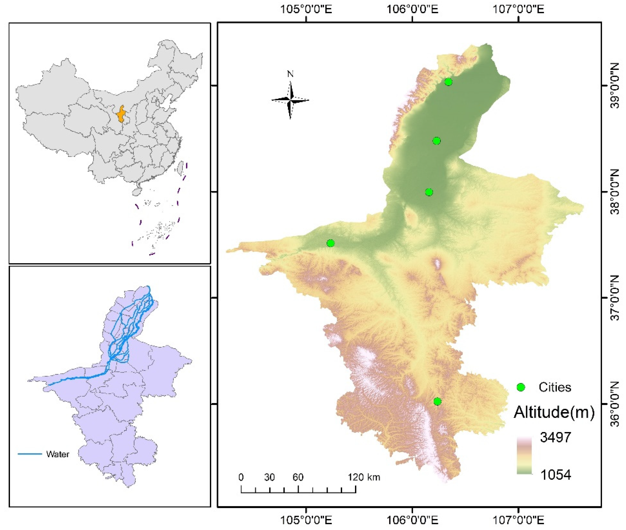
2.1. Study Area

This study was undertaken in Ningxia, a northwest province of China, bounded by Gansu Province, Shaanxi Province, and Inner Mongolia, covers the total area of about 66,400 km² extending from longitude 105°45′ E to 107°00′ E and latitude 38°20′ N to 39°30′ N [24] (Figure 1). Ningxia experiences average summer temperatures ranging between 17 and 24 °C and average winter temperatures dropping to between −7 and −15 °C [25]. Seasonal extreme temperatures can reach 39 °C in summer and −30 °C in winter with annual rainfall between 190 to 700 millimeters [26]. An arid to semiarid climatic pattern is visualized in the majority of counties except for the Yellow River basin which flows 397 km around 12 counties in the province [27]. Civilization is principally around the Yellow River and its tributaries and nearly half the GDP of the province is based on the production of grains and agricultural output value carried out in this basin while the rest of the area is of grasslands due to its semiarid climate [28]. The province has 22 county-level divisions for administrative purposes with 5 prefectural cities and the population is estimated to be around 7 million [29].

2.2. Data Used

We used Level-1 Landsat ETM+ (Enhanced Thematic Mapper) and OLI (Operational Linear Imaging) satellite imagery covering the study area for the years 2005, 2010, 2015, and 2020 with a 30 m resolution, obtained on the dates of 12 August 2005, 16 August 2010, 1 September 2015, and 13 August 2020, respectively. These datasets were acquired from the United States Geological Survey (USGS) portal [30]. The MODIS data were corrected for radiometric errors and downloaded from the National Aeronautics and Space Administration (NASA) earth data search portal with a resolution of 500 m for green and 250 m for red and near-infrared bands for the dates 21 August 2005, 15 August 2010, 21 August 2015, and 20 August 2020 [31]. The MODIS data were resampled to 250 m to reduce the computation difficulty and projected onto the common Universal Transverse Mercator (UTM) map projection system [32].

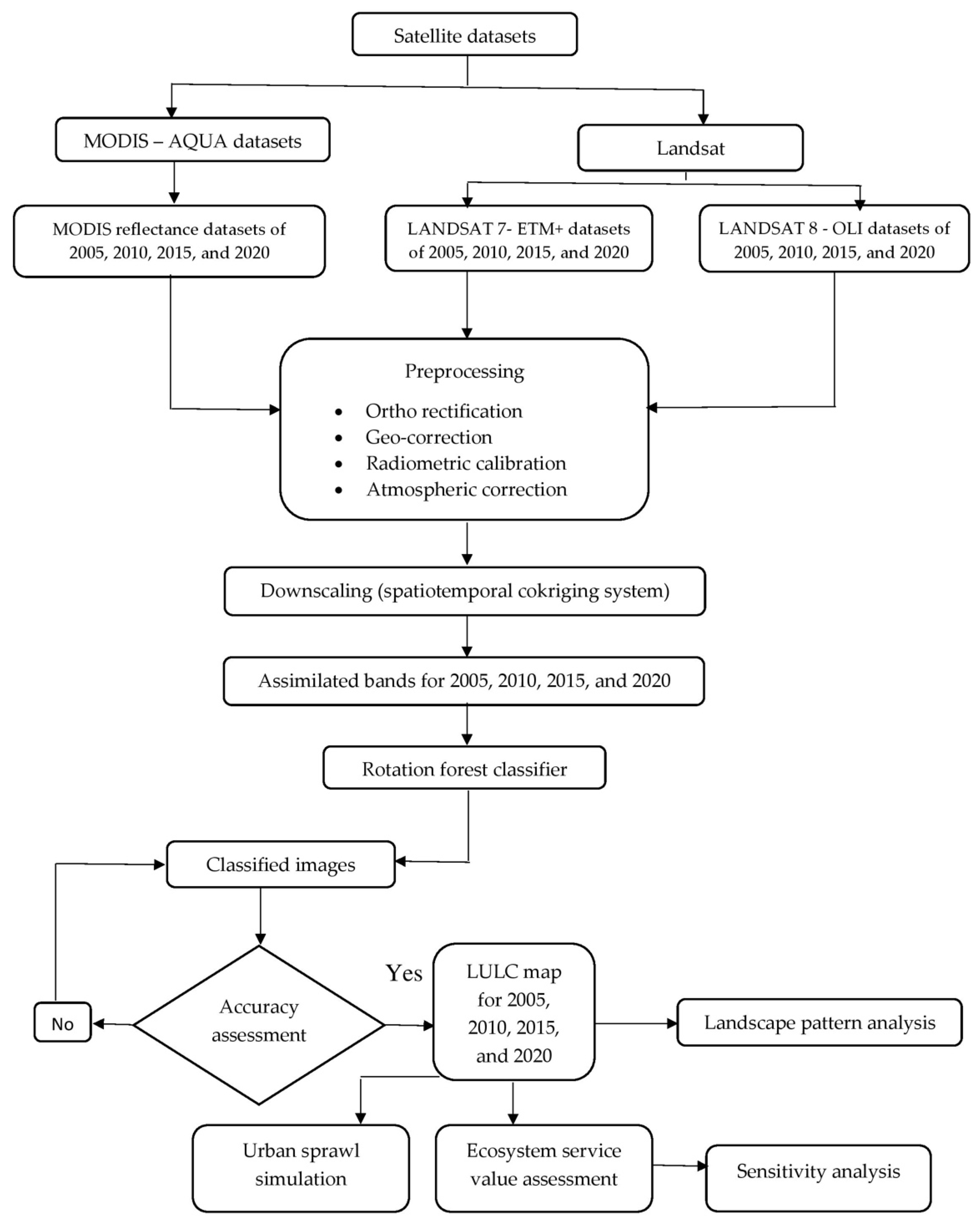
2.3. Research Design

To summarize our research design, we drew a schematic representation for the methodological framework used in this study (Figure 2), which is explained in the following subsections.

2.4. Satellite Data Preprocessing

We performed preprocessing of the images to obtain an accurate representation of the original scene by eliminating the various geometric and radiometric error sources that occurred during the acquisition of the data. Due to the failure of the scan-line corrector (SLC) in Landsat sensors from 2003, imageries obtained from 2005 and 2010 had data gaps, but they were still beneficial and upheld the same geometric and radiometric corrections; these imageries should be treated with Landsat 7 SLC off-gap function to fill the missing pixels then histogram correction can be used to rectify the filled data [33].

At first, geometric distortions occurred primarily because of variations in the altitude, velocity of the sensor platform, panoramic distortion, and earth curvature, and the atmospheric refraction was rectified [34]. Systematic distortions were corrected by deskewing while random distortions were corrected using well distributed GCP’s.

Next, we performed radiometric correction (conversion of digital number (DN) of the scene to reflectance values) and atmospheric correction (obscured fine details) by using the FLAASH modules and providing the elevation, scene center coordinates, sensor type, flight date and time, and information about the aerosol distribution, visibility, and water vapor condition as input from ancillary data. A topographic correction was applied to the MODIS datasets after extracting the reflectance data by the slope-match technique, which can be used to correct the disparities that arise due to very low sun angle and very low illumination in steep terrain. Once corrections were applied, the datasets could be used for further manipulation and analysis to extract data. We implemented all the atmospheric corrections and radiometric corrections in R software [35].

2.5. Image Fusion—Downscaling

Downscaling is a task performed to improve the resolving ability of any dataset. We used MODIS datasets as the coarse resolution data, and Landsat ETM+ and OLI datasets as fine resolution data to assimilate the data with a high spatial and temporal frequency. Consider the spatiotemporal (ST) cokriging system linear equation [36]

$$C\lambda =b$$

(1)

where λ consists of optimal coefficients ${\alpha }_{ij }$ and ${\beta }_{kl}$ to be estimated, b is a vector consisting of cross-variances between measured pixels, and C is the covariance matrix consisting of three elements with spatiotemporal functions. [14].

1. $C_p^{ij}$ is an N_i × N_j covariance matrix between the primary variable Z₁ at time t_i and t_j.

2. $C_{pc}^{ij}$ is an N_i × M_j cross-covariance matrix between the primary variable Z₁ at time t_i and the secondary variable Z₂ at time v_j.

3. $C_c^{ij}$ is the M_i × M_j covariance matrix between the secondary variable Z₂ at time v_i and v_j.

$${\widehat{Z}}_1(x_0, t_0)={{\displaystyle \sum }}_{i=1}^T·{{\displaystyle \sum }}_{j=1}^{N_i}{\alpha }_{ij}{Z}_1\left(s_{ij},t_i\right)+{{\displaystyle \sum }}_{k=1}^V·{{\displaystyle \sum }}_{l=1}^{M_k}{\beta }_{kl}{Z}_2\left(u_{kl},v_k\right)$$

(2)

where $\widehat{Z}$₁(x_0, t₀) is the predicted value for the pixel in the search window for the x₀ pixel at time t₀, $Z_1\left(s_{ij},t_i\right)$ is the primary variable for the $s_{ij}$ location at time $t_i$, and $Z_2\left(u_{kl},v_k\right)$ is the covariable for the $u_{kl}$ location at time $v_k$. The optimal coefficient of the Lagrange multipliers ${\alpha }_{ij }$ and ${\beta }_{kl}$ are determined using Equation (1), then the ST cokriging predictor ($\widehat{Z}$₁(x₀, t₀)) algorithm (Equation (2)) can be used to prepare the assimilated data by running a window of any desired size that is used by varying x₀ in the spatial domain at a certain time scale t₀. Another advantage is that the uncertainty estimate of the predicted value is also given in the form of a cokriging variance [37].

The assimilation was performed over the preprocessed 30 m resolution Landsat data with 250 m resolution MODIS data for three bands, namely, green, red, and NIR bands, with MODIS reflectance bands as primary variables and Landsat ETM+ and OLI bands as secondary or covariables, respectively. We first created an empirical spatial and temporal semi variogram using the observation, by creating a pixel pair between primary and covariable. Next, we fitted the semi variogram against the spatial lag to obtain the variance from the intercept, thereby obtaining all spatial–temporal cross-covariance functions in the covariance matrix namely $C_p^{ij}$, $C_{pc}^{ij}$, and $C_c^{ij}$ between Z₁ and Z_2. Next, a predictor window was allowed to run over the primary variable to obtain the ST cokriging-assimilated data [38]. All three assimilated bands were preserved to prepare the composites, to prepare the LULC map, and to portray the US. The two main things to consider in image fusion are that (i) the optimal color and spatial details must be separated and (ii) the spatial information should be manipulated to allow the adaptive enhancement of images. In order to check the accuracy of downscaling MODIS data from 250 m to 30 m, we used the root-mean-square Error (RMSE) model.

2.6. LULC Classification

We separated the landscape into six LULC classes (built-up area, woodland, farmland, grassland, water bodies, and unused land;

Table 1. Description of LULC classes.

ID	LULC Classes	LULC Description
1	Built-up area	Roads, man-made structures (stadiums, parks, and urban areas)
2	Woodland	Dense vegetation, forest and timberland
3	Farmland	Agriculture and productive lands
4	Unused land	Drylands, nonproductive lands, and nonirrigated lands
5	Water bodies	Rivers, streams, lakes, open water, and ponds
6	Grassland	Grazing area, bushes, and shrubbery

) which were the major parameters to evaluate ES and economic values [1,4,16], and we used a rotation forest (RF) classifier, which is a machine-learning-based classifier ensemble based on a feature extraction technique and it uses a decision tree approach with two parameters, i.e., number of iterations and splits, specified by the users to obtain enhanced predictive performance with fewer trees [39]. The steps involved in the RF algorithm are: (i) the total area is partitioned into k subsets based upon homogeneity; (ii) a principal component analysis (PCA) is applied on every subset to identify the relationships between subsets (i.e., variability information); (iii) the rotation matrix is formed with the coefficients of the obtained vectors and the accuracy of the RF algorithm depends on how well the rotation matrix is constructed with the linear transformed subsets [1].

We prepared an LULC map using assimilated data with six classes as shown in Table 1 and compared the LULC changes from 2005 to 2020. To assess the accuracy of classification we used Google Earth images obtained from the Google Earth Engine (GEE) gateway, a sample of 25 random points was selected for every class, and values were generated. The accuracy of the LULC map should be greater than 85% or a kappa coefficient greater than 0.7 to be acceptable [40]; we computed user and producer accuracy using a confusion matrix and the overall accuracy by using kappa in ERDAS IMAGINE to examine the accuracy of the classified LULC map [41].

2.7. Landscape Pattern Evaluation

2.7.1. Landscape Metrics

We used eleven landscape metrics to examine the landscape pattern information and characteristics of its structure and spatial configuration between 2005 and 2020 (

Table 2. Spatial metrics computed to examine the landscape patterns information.

Landscape Metrics	Formulas	Explanation	Values Range
Patch type area	$CA={\displaystyle {\displaystyle \sum }_{j=1}^n}{a}_{ij }\left(\frac{1}{\mathrm{10,000}}\right)$ aij = area measures in m2 of patch covering ij.	To quantitate the area of every patch in any particular class	CA > 0
Patch area ratio	$PLAND=P_{i }=\frac{{{\displaystyle \sum }}_{j=1}^n{a}_{ij}}{100}\left(100\right)$ Pi = total landscape occupied by different patches aij = area measures in m2 of patch covering ij	To proportionate the different landscape patches to the area of a patch	0 < PLAND ≤ 100
Number of patches	$NP=n_i$ ni = total number of patches in the region of patch type i	To quantify the number of the different patches present in the LULC map	NP ≥ 1
Landscape shape index	$LSI=\frac{e_i}{min e_i}$ ei= length of the different edges	To quantify relative amount of patch perimeter to landscape area	LSI 1 ≥ 1, without limit
Clumpiness index	$Clumpy=\left[(G_i-P_i\right)/P_{i }for G_{i }<P_i \& P_i$ < 5, else $G_i-P_i / 1-P_I$] gii = total number of similar connections among pixels, i based doubled progression and gik = total number of similar connections among pixels, k based doubled progression Pi = total landscape occupied by different patches	To depict the adjacency deviations from random distribution. Clumpiness shows the dispersion of patches in the map	−1 ≤ CLUMPY ≤ 1
Patch density	$PD=\frac{n_{i }}{A}\left(10,000\right)$ ni = total number of patches in the region of patch type i A = total area in the landscape measures in m2	To calculate density between every patch type in an image	PD > 0
Largest patch index	$LPI=\frac{ma{x}_{j=1 }^n\left(a_{ji }\right)}{A}\left(100\right)$ aij = area measures in m2 of patch covering ij A = total area in the landscape measures in m2	To get a percentile of the landscape comprised by the major patch in particular level	0 < LPI ≤ 100
Average patch area	$MN=\frac{{{\displaystyle \sum }}_{j=1}^n{X}_{ij}}{ni}$ ni = total number of patches in the region of patch type i	To examine the average area patches in a level	0 < MN ≤ 100
Shannon evenness index	$SHEI={\displaystyle {\displaystyle \sum }_i^m}\left(P_{i }\ast lnln (P_{i } \right))/ln\left(m\right)$ Pi = total landscape occupied by different patches m = total number of patch classes	To delineate the patches with high diversity	0 ≤ SHEI ≤ 1
Shannon’s diversity index	$SHDI={\displaystyle {\displaystyle \sum }_{i=1}^m}\left(P_{i } lnln P_{i } \right)$ Pi = total landscape occupied by different patches m = total number of patch classes	To portray the amount of information for every patch area	SHDI ≥ 1
Contagion index	$Contag=[1+{\displaystyle {\displaystyle \sum }_{i=1}^m}·{\displaystyle {\displaystyle \sum }_{k=1}^m}[\left(p_{i }\right)\{g_{ik}/{\displaystyle {\displaystyle \sum }_{k=1}^m}{g}_{ik}\}\{ln\left(p_i\right)[g_{ik}/{\displaystyle {\displaystyle \sum }_{k=1}^m}{g}_{ik}]/2ln \left(m\right) ]100$ gik = total number of similar connections among pixels, k based on doubled progression Pi = total landscape occupied by different patches m = total number of patch classes	To deduce the percentage of aggregation or clumpiness between patch types	Percent < Contag ≤ 100

). Landscape metrics (LM) are indices used to depict the map patterns influenced by biological and physical infrastructures [42]. LM exist in three levels, namely, patches, patch type, and landscape-level to detect and quantify spatial configuration patterns. The spatial configuration and composition affect the landscape ecology independently thus playing an influential role in land-use planning [43]. We identified and used eleven landscape metrics from different conceptual classes such as shape metrics, diversity metrics, and edge metrics to portray the landscape spatial configuration changes with its attribute between 2005 and 2020 for Ningxia Province using the FRAGSTATS package (Version 4.2). We used metrics such as patch type area (CA), patch area ratio (PLAND), number of patches (NP), landscape shape index (LSI), clumpiness index (CLUMPY), average patch area (AREA_MN), patch density (PD), largest patch index (LPI), Shannon diversity index (SHDI), Shannon evenness index (SHEI), and contagion index (CONTAG), to examine the landscape patterns in the LULC map.

2.7.2. Land-Use Degree

We used land-use degree (LUD) to conceptualize the degree of change of the landscape from one period to another based on the principle of how the land has evolved by human intervention and its consequences. A higher LUD indicates the landscape has undergone several changes which are unrecoverable and vice versa for lower degrees; the degree changes based on the human’s impact on natural landscapes are:

$$L_{\mathrm{u}}=100\times {\displaystyle \sum }_{i=1}^n\left(P_{\mathrm{i} }\times Q_{\mathrm{i} }\right)$$

(3)

where L_u is the index of LUD; $P_{\mathrm{i} }$is the grade I land-use degree grading index; and $Q_{\mathrm{i} }$is the percentage of LUD area.

2.8. Evaluation of Ecosystem Service

In general, LULC changes affect the process in the ecosystem lacking a sustainable development mechanism, thus the ecosystem service values (ESV) are also affected. We used a benefit transfer approach for the quantitative assessment of ecosystem service values for the whole of China; the elasticity economic ESV coefficient is computed by the formula:

$$V{C}_0=\frac{1}{7}\times P\times \frac{1}{n}{\displaystyle \sum }_{i=1}^n Q_{i }$$

(4)

where VC₀ is the value of the ESV equivalent factor (yuan km⁻² a⁻¹), the yuan (¥) is the monetary unit of China; P is the average grain price that varies for every year (yuan × kg⁻¹); Q is the average grain yield for every year (kg × km⁻²); and n is the number of years taken into consideration. The services available in the ecosystem for every class type were identified and a monetary value for any particular service based on socioeconomic conditions was provided for Ningxia Province; we used Formula (5) to compute ESV for every service:

$$ESV={\displaystyle \sum }_{k=1}^n\left(A_{k }\times V{C}_{k }\right)$$

(5)

where ESV is measured in yuan; $A_{k }$is the area in hm² of landscape type K; and $V{C}_{k }$is the ESV coefficient of that landscape (yuan km⁻² a⁻¹).

2.9. Sensitivity Analysis

Since the ESV do not effectively conjoin the LULC classes, there is some uncertainty in the value of the coefficient (VC), so the level of dependence of ESV upon the coefficient value was determined using the sensitivity analysis based upon the standard elasticity concept. We used Equation (6) to compute the coefficient of sensitivity (CS):

$$CS=\left|\frac{\left(ES{V}_{j }-ES{V}_{i }\right)/ ES{V}_{i }}{\left(V{C}_{jk }-V{C}_{ik }\right)/ V{C}_{ik } }\right|$$

(6)

where CS is the coefficient of sensitivity; ESV is ecosystem service values; VC is the ecological value coefficient; i and j are the initial value coefficients, and the adjusted coefficients; and k stands for different LULC classes. If CS > 1, then the ESV coefficient estimated is said to be elastic; if CS < 1, then the estimated ESV coefficient is inelastic thus, if any changes in the value of the coefficient in any proportion, then the ESV coefficient is also altered according to that proportion; in the case of a prominent alteration amount, then there must be more seriousness in the usage of a precise ESV coefficient.

2.10. Monitoring and Simulation of Urban Sprawl

2.10.1. Monitoring the Urban Sprawl

The uncontrolled and unplanned development of infrastructures on the fringes of the urban area is called urban sprawl and is also referred to as leapfrog development. US and ESV are negatively correlated, thus by using the US simulated model, the areas having a high sensitivity index for ESV must be handled with severe attention to reduce the ecological environmental damages. We used Renyi’s entropy to monitor the US in Ningxia Province, based on the dispersion level of urban areas. The RE value ranges between 0 and 1 from highly dense distributed area to dispersed distribution; RE was computed using the Equation (7):

$$H_{\alpha }=\frac{1}{1-\alpha } ln{\displaystyle \sum }_{i=1}^N{P}_i^{\alpha }$$

(7)

where N is the total number of patches for built-up and non-built-up areas in the aggregated LULC map, P_i is the corresponding perimeter in the LULC map, and$H_{\alpha }$is the Renyi’s entropy value calculated with condition $\alpha \ge$1 and $\alpha \ne 0$.

2.10.2. Simulation of Urban Sprawl

For the simulation of the US, we used a land-change modeler available in TerrSet (formerly IDRISI) software. Initially, we calibrated the land-change modeler by quantifying the LULC changes for the years 2005, 2010, and 2015. Then, we obtained the LULC changes map using transition modelling and the change probability grid was also obtained for 2015 and 2020. Next, the urban extent prediction model utilizing a Markov chain [44,45,46] was used to calibrate the change probability grid with the LULC map by using certain reference data for 2005–2020.

Then, the predicted urban extent for 2020 was compared with the original 2020 LULC map with kappa coefficients; if an acceptable accuracy was obtained then the urban extent of 2025 could be simulated, by considering the 2020 urban extent as the base and computing the simulated 2025 extent by combining the change map and change probability grid between 2020 and 2025 using the calibrated and validated urban extent and prediction modeler.

3. Results

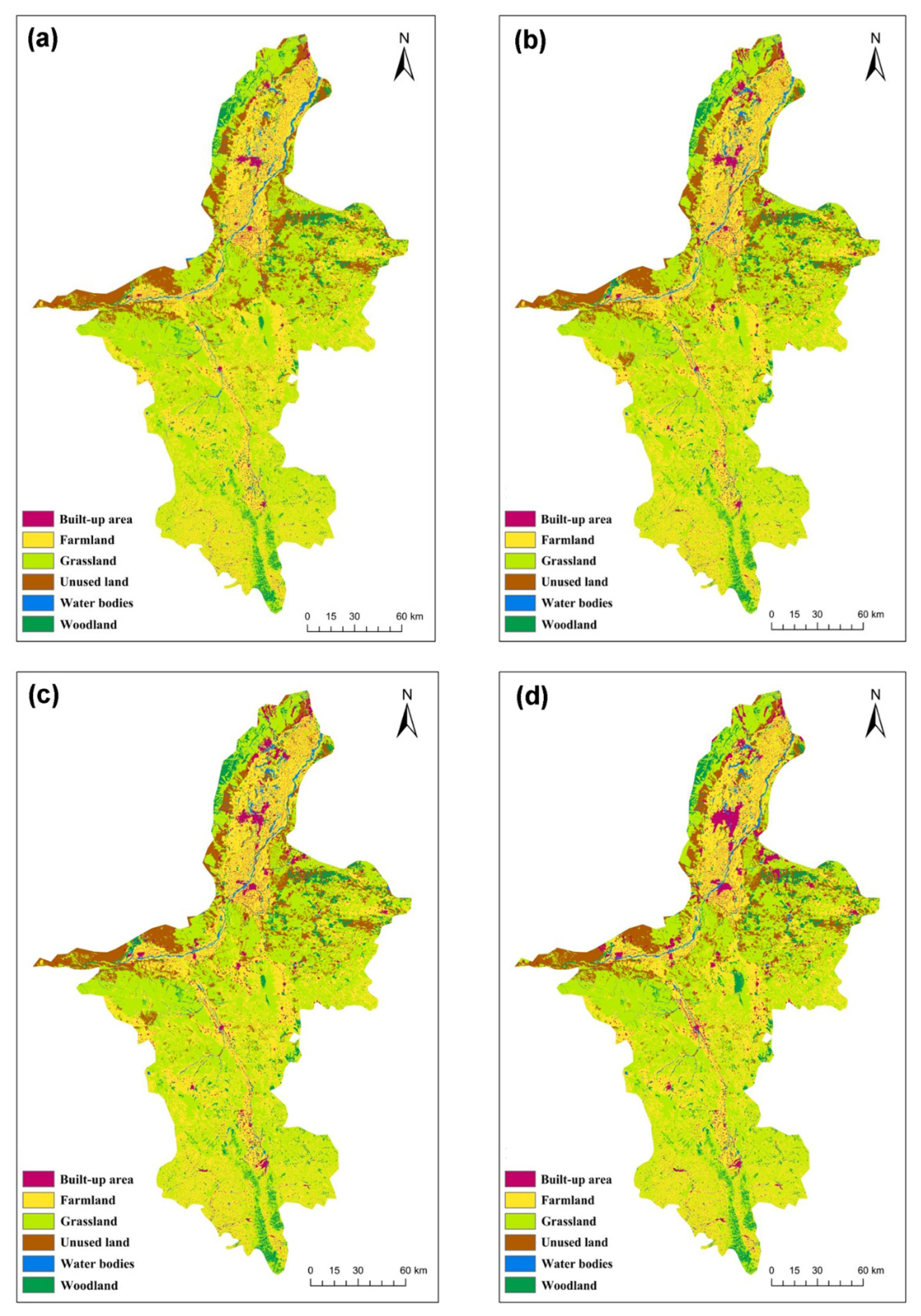
3.1. Evaluation of Landscape Changes

The accuracy of the downscaled MODIS dataset concerning Landsat 8 images exhibited a high accuracy with 0.90 for green, 0.93 for red, and 0.92 for NIR bands (

Table 3. Accuracy of assimilated datasets with respect to Landsat 8 reference image.

Band	Correlation Coefficient	Reflectance RMSE
Green	0.905	1.235
Red	0.934	1.47
NIR	0.924	1.364

). The LULC map (Figure 3) prepared by down sampling the data exhibited a greater accuracy with an overall accuracy of 88.3, 89.9, 87.3, and 87.9, and a kappa coefficient of 0.86, 0.88, 0.87, and 0.86 over the period of 2005, 2010, 2015, and 2020, respectively (

Table 4. Accuracy assessment values for the LULC using downscaled images by 2005, 2010, 2015, and 2020. Producer accuracy = PA; user accuracy = UA.

	2005		2010		2015		2020
Classes	PA	UA	PA	UA	PA	UA	PA	UA
Built-up area	82.2	83.9	90.2	87.2	88.6	84.4	89.1	84.5
Woodland	88.7	89.6	89.5	86.9	90.7	90.3	88.5	90.3
Farmland	90.7	93.8	88.3	90.2	91.2	93.2	87.6	88.6
Unused land	91.6	94.8	89.6	92.1	88.1	91.8	90.2	90.7
Water bodies	93.1	89.9	90.6	93.5	81.6	82.6	84.1	86.1
Grassland	93.1	95.1	92.7	93.8	83.3	84.2	90.5	94.6
Overall accuracy	88.3		89.9		87.3		87.9
Kappa	0.86		0.88		0.87		0.86

). When the kappa coefficient was greater than 0.85, then that particular LULC map could be used as a reference for any purposes or analysis, so we used this LULC map for the study of sensitivity analysis, ESV, and US results.

By analyzing the trend of the landscape terrain over a time frame of 2005–2020 in Ningxia Province, the farmland areas kept on reducing with a difference of 1,349,222 hectares (

Table 5. Land-area conversion and its specific percentage of each class of LULC during the study period (2005–2020).

Landscape	2005		2010		2015		2020
Type	Area	%	Area	%	Area	%	Area	%
	(km2)		(km2)		(km2)		(km2)
Farmland	17,593.254	33.84	17,817.687	34.27	17,892.768	34.41	23,665.578	45.52
Grassland	24,164.758	46.48	23,672.548	45.53	23,424.158	45.06	21,152.917	40.69
Woodland	2651.662	5.10	2780.862	5.34	2779.086	5.34	511.174	0.98
Built-up area	1184.49	2.27	1698.711	3.26	2026.928	3.89	2969.329	5.71
Water bodies	971.773	1.86	982.577	1.89	997.525	1.91	1204.207	2.31
Unused land	5417.804	10.42	5031.542	9.67	4863.013	9.35	2480.272	4.77
Total	51,983.743	100	51,983.743	100	51,983.743	100	51,983.743	100

), while the woodlands were rapidly growing with a change of around 956,805 hectares. The spatial distribution of grassland, water bodies, and unused land terrain were mostly undisturbed, while the urban landscape area was enlarged four times during the time frame, resulting in increased impervious layers.

3.2. Evaluation of Landscape Pattern

Landscape metrics were computed for every six LULC categories and are tabulated as shown in

Table 6. Change of LULC in Ningxia over 15 years (2005–2020), based on different landscape metrics.

Landscape Type	Year	Patch Type Area	Patch Area Ratio	Number of Patches	Patch Density	Max Patch Index	Landscape Shape Index	Mean Patch Area	Concentration
		CA	PLAND %	NP	PD	LPI	LSI	MN hm2	CLUMPY
		hm2
Farmland	2005	1,759,325.40	33.84	10,296	0.20	6.22	207.88	170.87	0.93
	2010	1,781,768.79	34.28	10,376	0.20	5.88	208.44	171.72	0.93
	2015	1,789,276.77	34.42	10,469	0.20	6.07	207.66	170.91	0.93
	2020	2,366,557.83	45.53	318,276	6.12	18.12	517.45	7.44	0.82
Woodland	2005	265,166.28	5.10	3705	0.07	0.25	99.57	71.57	0.94
	2010	278,086.23	5.35	3817	0.07	0.25	100.76	72.85	0.94
	2015	277,908.66	5.35	3882	0.07	0.21	100.70	71.59	0.94
	2020	51,117.48	0.98	10,041	0.19	0.12	93.16	5.09	0.88
Grassland	2005	2,416,475.88	46.49	3119	0.06	33.98	195.25	774.76	0.93
	2010	2,367,254.88	45.54	3506	0.07	27.52	195.61	675.20	0.93
	2015	2,342,415.78	45.06	3800	0.07	28.49	196.27	616.43	0.93
	2020	2,115,291.78	40.69	176,357	3.39	12.50	542.48	11.99	0.81
Water bodies	2005	97,177.32	1.87	975	0.02	0.65	73.96	99.67	0.93
	2010	98,257.77	1.89	1217	0.02	0.52	83.83	80.74	0.92
	2015	99,752.58	1.92	1353	0.03	0.53	84.60	73.73	0.92
	2020	120,420.72	2.32	19,954	0.38	0.57	137.82	6.03	0.88
Built-up area	2005	118,449.00	2.28	5952	0.11	0.18	98.00	19.90	0.91
	2010	169,871.13	3.27	6376	0.12	0.24	103.78	26.64	0.92
	2015	202,692.87	3.90	6596	0.13	0.26	103.40	30.73	0.93
	2020	296,932.95	5.71	82,044	1.58	0.68	203.59	3.62	0.88
Unused land	2005	541,780.47	10.42	1991	0.04	1.46	82.06	272.11	0.96
	2010	503,154.27	9.68	2306	0.04	1.35	87.69	218.19	0.96
	2015	486,301.32	9.35	2410	0.05	1.31	88.23	201.78	0.96
	2020	247,879.80	4.77	54,977	1.06	0.59	233.47	4.51	0.85

. The patches count changed significantly under every circumstance irrespective of their class and the patch density was related to the total number of patches directly along with the patch area ratio for every class. The patch type area increased for classes such as woodland, built-up areas, and water bodies while the trend was declining in the case of grassland, farmland, and unused land for 15 years between 2005 and 2020. The LSI value was primarily dependent on landscape changes occurring over the time frame, i.e., farmland, grassland, and unused land were showing downtrends and the trend was upward in the case of woodland, built-up areas, and water bodies.

The mean patch area showed that when the landscape change was abrupt, in certain cases MN increased. The maximum patch index (LPI) increased over a decade and was followed by a slight decrease in trend in the next quarter for grassland, farmland, and built-up areas while woodland exhibited exactly the opposite trend. Water bodies had LPI increasing over the time frame and the unused land had LPI declining over the years. The clumpiness, an aggregated index between the changes and all the classes, showed a downtrend oscillation, which was found only in the case of the barren landscape.

The aggregated table shows the different metrics evaluated between 2005 and 2020, from which we infer an increase in the number of patches by 3204, patch density by 0.55, and LPI by 8% (

Table 7. Aggregate changes on LULC in Ningxia over 15 years (2005–2020), based on different landscape metrics.

Year	Number of Patches	Patch Density	Maximum Patch Index	Landscape Shape Index	Mean Patch Area	Contagion Index	Patch Richness	Shannon Diversity Index	Shannon Evenness Index
	(NP)	(PD)	(LPI %)	(LSI)	(hm2)	(Contag)	(PR)	(SHDI)	(SHEI)
2005	26,038	0.50	33.98	165.50	199.65	58.58	6	1.27	0.71
2010	27,598	0.53	27.52	168.97	188.36	57.74	6	1.29	0.72
2015	28,510	0.55	28.49	169.52	182.33	57.36	6	1.31	0.73
2020	661,649	12.73	18.12	414.06	7.86	55.93	7	1.17	0.65

). The Shannon diversity value increased significantly while the evenness index showed stabilized values in the first decade followed by increased values. The mean patch area and contagion index also increased but the richness values remained constant.

3.3. Ecosystem Service Values

ESV show the impact of landscape changes on the ecosystem in the form of monetary value as shown in

Table 8. Value and change of ecosystem services in the landscape types from 2005 to 2020.

Landscape Type	ESV/× 105 (RMB/a)				2005–2010		2010–2015		2015–2020		2005–2020
	2005	2010	2015	2020	Change	Rate	Change	Rate	Change	Rate	Change	Rate
					(Yuan)	%	(Yuan)	%	(Yuan)	%	(Yuan)	%
Woodland	51,267.25	53,765.19	53,730.86	9883.05	−2497.94	−4.87%	−34.33	−0.06%	−43,847.81	−81.61%	−41,384.19	−80.72%
Grassland	154,811.53	151,658.18	150,066.87	135,516.17	3153.34	2.04%	−1591.32	−1.05%	−14,550.70	−9.70%	−19,295.36	−12.46%
Farmland	107,570.43	108,942.69	109,401.75	144,698.45	−1372.26	−1.28%	459.06	0.42%	35,296.70	32.26%	37,128.01	34.52%
Water bodies	39,528.24	39,967.72	40,575.76	48,982.81	−439.49	−1.11%	608.03	1.52%	8407.06	20.72%	9454.58	23.92%
Unused land	2012.17	1868.71	1806.12	921.17	143.46	7.13%	−62.59	−3.35%	−884.95	−49.00%	−1091.00	−54.22%
Total	355,189.62	356,202.50	355,581.36	340,001.65	−1012.89	−0.29%	−621.14	−0.17%	−15,579.70	−4.38%	−15,187.96	−4.28%

. The built-up areas generally do not have any ESV, so built-up areas were neglected in this analysis. In the context of sustainable development, ESV should be of the stabilized form; our evaluation results showed an increase in the value for water bodies and farmland and ESV declined for woodland, grassland, and unused land. Overall, the ESV change was −4.28 %, with an increment in the value of about 15,187.96 × 105 yuan in 15 years. In our study of the assessment of landscapes, the ESV of woodland decreased by −41,384.19 yuan with a rate of change of −80.7%. Grassland had the ESV fall off to 19,295.3 × 105 yuan at the decreasing rate of 12.46%. Farmland ESV increased by 34.5% with a monetary value of around 37,128.01 × 105 yuan. Water bodies exhibited a surge in ESV by 9454.58 × 105 yuan at the rate of 23.92%. Unused land had the most decreased ESV by 54.2% with an equivalent shrinkage of 1091 × 105 yuan.

The ESV on various ES are shown in

Table 9. Changes in the ecosystem service values (ESV) during the 15 years of the study period (2005–2020) in Ningxia.

Ecosystem Services	ESV/× 105 (Yuan/a)				2005–2010		2010–2015		2015–2020		2005–2020
	2005	2010	2015	2020	Change	Rate	Change	Rate	Change	Rate	Change	Rate
					(Yuan)	%	(Yuan)	%	(Yuan)	%	(Yuan)	%
Gas conditioning	33,101.69	33,252.67	33,104.55	27,026.91	150.9849499	0.46%	−148.1200283	−0.45%	−6077.642231	−18.36%	−6074.77731	−18.35%
Climate regulation	39,830.10	39,927.91	39,791.06	37,194.19	97.8136092	0.25%	−136.8516981	−0.34%	−2596.87594	−6.53%	−2635.914029	−6.62%
Water conservation	51,622.43	51,943.58	52,067.67	50,767.03	321.1486492	0.62%	124.0920275	0.24%	−1300.633524	−2.50%	−855.3928475	−1.66%
Soil formation and protection	73,680.09	73,559.84	73,219.25	68,891.43	−120.2494028	−0.16%	−340.5822689	−0.46%	−4327.823156	−5.91%	−4788.654828	−6.50%
Waste disposal	72,297.13	72,372.43	72,430.38	78,849.93	75.30526818	0.10%	57.94361298	0.08%	6419.550865	8.86%	6552.799746	9.06%
Biodiversity conservation	45,778.76	45,725.32	45,510.03	40,142.54	−53.44034607	−0.12%	−215.2886982	−0.47%	−5367.497104	−11.79%	−5636.226148	−12.31%
Food production	22,352.36	22,429.28	22,429.45	26,731.41	76.91105151	0.34%	0.17300232	0.00%	4301.958869	19.18%	4379.042923	19.59%
Raw materials	8734.05	9029.49	9021.20	4215.97	295.4381675	3.38%	−8.28795204	−0.09%	−4805.234161	−53.27%	−4518.083945	−51.73%
Entertainment culture	7793.01	7961.98	8007.76	6182.25	168.9744733	2.17%	45.77713704	0.57%	−1825.508276	−22.80%	−1610.756666	−20.67%
Aggregate	355,189.62	356,202.50	355,581.36	340,001.65	1012.88642	0.29%	−621.1448656	−0.17%	−15,579.70466	−4.38%	−15,187.9631	−4.28%

for the span of 15 years between 2005–2020. The results reveal that ESV for food production increased by 19.59% with a yield of 4379.04 × 105 yuan and climate-regulating services had the surge of 2635.9 × 105 yuan at the rate of 6.62%. Overall, the change of ESV was 15,187.96 × 105 yuan with a surge of 4.28%. By assessing the ESV in every quarter of our study, the maximum change of 100% was between 2015 and 2020, with the highest gain in the raw material services of 53.27%. The ESV gain of every service area accounted for in this research was sorted as climate regulation, entertainment culture, biodiversity conservation, waste disposal, water conservation, soil formation and protection, gas conditioning, and raw materials.

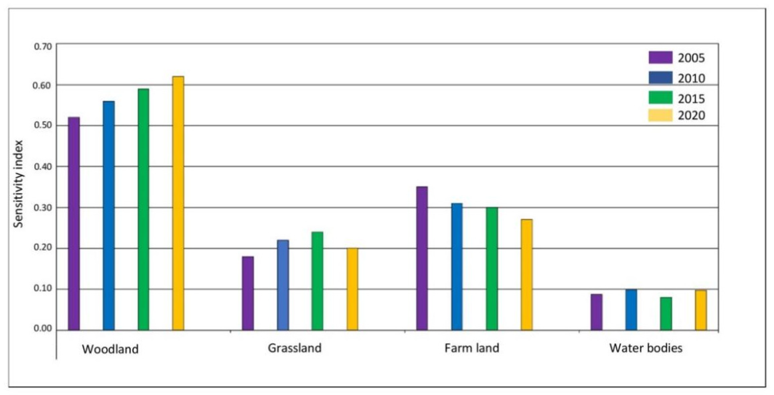
3.4. Sensitivity Analysis

The sensitivity index (CS) of different landscapes was below the range of 0.65 in the Ningxia Province for the years between 2005 and 2020 (Figure 4). Woodland had the highest sensitivity index value of 0.62 in 2020 and all the remaining landscapes had a value below 0.5. The sensitivity index portrays the reliability of ESV on LULC classes. If the value is below 1, then the ESV coefficient estimated is unchangeable with respect to its economic value; moreover, the study revealed the same, i.e., CS < 1, so the ESV estimated for different landscapes are credible with more reliability.

3.5. Level and Simulation of Urban Sprawl

US level was assessed by Renyi’s entropy. The entropy value for Ningxia Province in 2005 and 2010 was 0.35 and 0.56, respectively, which revealed the presence of fewer aggregated settlements, whereas in 2015 and 2020 the entropy values swelled by 0.78 and 0.91, respectively, showing dispersed settlements with a high level of encroachment along the urban fringes. This sustainable development is not feasible and leads to a strain on several multiutility services such as sewage management and drinking water facilities to the public.

The kappa coefficient between the classified and modelled LULC map was 84.8%, which was enough for obtaining a high-level accuracy in simulating the US using an urban extent prediction modeler. The predicted model of 2025 showed that the urban extent will be increased by 15.5%, leading to an increase in impervious layers, thereby resulting in a lack of ecosystem service value.

3.6. Effects of Urban Sprawl on ESV

The US and ESV are negatively correlated to each other, and the analysis revealed the same: as the US increased, the ecosystem values fell off to certain proportions. From 2005, after the fringes began to develop, the negative contribution of US on ESV was at the rate of 5.89% and increased to 27.89% in 2020 (

Table 10. Effects of ESV loss in consideration to the US from 2005 to 2020.

Effects	2005	2010	2015	2020
Urban expansion (km2)	20,566.87	26,487.69	31,897.25	35,478.25
Value loss (×105 yuan)	1567	2497	3189	3678
Contribution rate	5.89	14.47	21.67	27.89

). The US in the ecologically important landforms such as farmlands, forests, and grasslands were the main reason for the decline in ESV, thus the US was the very sensitive factor of ESV. US cannot be contained but should instead be mitigated by proper land-use planning by skipping out the water bodies and conservational landforms in the order of unused land, grassland, and woodland, thereby reducing the ESV loss.

4. Discussion

Our findings showed the degree of changes in the landscape pattern during the period 2005–2020 in Ningxia Province using the LULC map prepared from the downscaled data. The results showed that the farmlands were transformed into woodland and urban landscape, leading to severe urbanization in urban fringes and construction booming, with a lack of basic amenities. Urbanization and its impact on the ecosystem resulted in a fall of ESV and a lack of multiutility services available to the public generating middle-class demands. Ningxia Province experienced landscape degradation in certain classes due to human intervention with an increase in the number of patches and aggregation between them. Landscape transformations in certain cases added an advantage to the area–species relationship due to the growth of woodlands and grasslands resulting in a high biodiversity ranking. The Shannon diversity and evenness index delineated the patches and portrayed the information about patches with a high diversity during the period between 2005 and 2020.

Overall, it is evident that ESV decreased by 15,187.9 × 105 yuan in Ningxia Province at a rate of 4.28%. Generally, ESV decreased due to urbanization as revealed by other studies on Shenzhen from 1996 to 2004 with a loss of 231.3 million yuan due to the development of infrastructures in existing woodlands and water bodies, and Qianyang County also experienced an ES value decrease from RMB 19.165 billion in 2002 to RMB 18.814 billion by 2012. [47]. However, in this research, ESV grew up due to the conversion of farmland into woodland and water bodies, although there was a loss of ESV due to the conversion of cultivable lands, increasing the demand for food, ESV being primarily dependent on cropping type and the system used in those lands, which has majorly changed in several provinces of China including Qianyang, Hainan Island, and Hunan. So, a local government must promote agricultural practices with environmentally friendly goods to increase the transformation of woodland and water bodies into farmlands by providing incentives or subsidies.

Primarily, the transformation of grassland, farmland, and water bodies into built-up areas is inevitable in a fast-developing country with a high population density, resulting in the severe downfall of ESV. The ES study in the Hang-Jia-Hu region (Chinese province) indicated a loss of RMB 8.5 billion ESV per year between 1994 and 2003 due to rapid urbanization, even though there was a gain in GDP [48]. To mitigate these adverse effects, a proper management of landscapes should be done. The conversion between the farmland, grassland, and water bodies into built-up areas must be carried out with less environmental impact encouraging construction using green products, and simultaneously, when the grassland or farmland is converted into built-up areas, then new grasslands or farmlands should be generated from unused land. According to the payment for ecosystem services (PES) proposed by Zhang et al. [49]., cash subsidies can be provided to motivate the rural poor farmers for certain schemes such as the conversion of cropland to forest program (CCFP) and the ecological welfare forest program (EWFP), which must be formulated by the Chinese government to prevent soil erosion and habitat loss. By similar approaches, grassland can be transformed into woodland because grasses are prone to fire, which in turn may result in an increase in greenhouse gas concentration, and soil provision services value may be reduced.

The ESV for climate regulation were highest, followed by water conservation and soil formation and protection service. Food production had the lowest proportion in the study due to the conversion of farmland into various landscapes. Since the grassland and woodland spatial area was increased, the services of climatic regulation and water conservation automatically increased on a regional scale. The sensitivity index between the ESV and LULC classes revealed that both factors were considered as credible since the CS value was below 1.

The negative impact of the US on ESV was studied and we inferred that around 28% declination of ESV was due to the formation of high-density urban expansion fringes around the urban areas. The US was of linear pattern and leapfrog pattern in certain cases, which were fragmented and complex over a certain period due to anthropogenic activities. The simulated US for 2025 can be used extensively by planners and administrators to mitigate the adverse effects of urbanization, which is expected to be 15.5%. Proper plan proposals can be developed for the sewage management system for the population residing on the fringes of urban areas, potentially preventing urban floods, and basic amenity and utility services can be provided by a proper study on location-allocation analysis. Stringent protocols can be formulated and enforced for the development of housing on fringes without causing harm to biodiversity.

5. Conclusions

Our study developed an LULC map from downscaled satellite images with proper validations followed by an evaluation of landscape pattern changes and examined ESV for every class and certain ES over the period 2005–2020. The US is another causative factor in consideration with ESV, and the US was predicted for 2025 for a proper planning of resources available. From this research, it is evident that the deterioration of the spatial pattern of landform was prevented to a certain extent in 2015–2020 due to various plans enforced by the government for landscape and biodiversity protection. However, the urban landscapes tended to be increased in larger proportions due to the high population density in certain areas. The structure of the landscape pattern was studied with its spatial representation and revealed those patches, and its spatial composition was altered based upon the trend of the LULC changes, as when LULC changes more, the patches count will increase accordingly.

The ESV of Ningxia Province were greater than the national average ESV due to the financial incentives provided by the government to enrich the province with floristic diversity, even though the urban landscapes were increasing. Food production services had the least ESV, while climate regulation service had the highest ESV in our research. The followed ESV can be applied all over the world, especially in Africa and Asia for calculating any grain production.

US is another sensitive factor of ESV; the Renyi’s entropy was 0.91 indicating the presence of high encroachment in fringes in 2020 with a loss of nearly 28% of ESV. The study was done primarily to envisage the LULC changes, depict the relationship between the causative factor responsible for those changes, plan developmental proposals at the landscape level, and maintain the economic benefits and ecological gains of the different land-cover classes to enhance their ESV for Ningxia Province, requiring an interdisciplinary and science-based approach. This image fusion approach to estimate the landscape changes was limited to small-scale areas due to the disparity in large-scale areas. Thus, future research should consider different fusion data sets to estimate the landscape changes and their impacts on ES.

References

1. Padmanaban, R.; Bhowmik, A.K.; Cabral, P. Satellite image fusion to detect changing surface permeability and emerging urban heat islands in a fast-growing city. PLoS ONE 2019, 14, e0208949. [Google Scholar] [CrossRef]
2. Feller, I.C.; Friess, D.A.; Krauss, K.W.; Lewis, R.R. The state of the world’s mangroves in the 21st century under climate change. Hydrobiologia 2017, 803, 1–12. [Google Scholar] [CrossRef] [Green Version]
3. Padmanaban, R. Land Use and Land Cover Mapping and Shore Line Changes Studies in Tuticorin Coastal Area Using Remote Sensing. Cloud Publ. Int. J. Adv. Earth Sci. Eng. 2012, 1, 1–12. [Google Scholar]
4. Khare, D.; Patra, D.; Mondal, A.; Kundu, S. Impact of landuse/land cover change on run-off in a catchment of Narmada river in India. Appl. Geomat. 2014, 7, 23–35. [Google Scholar] [CrossRef]
5. Bhat, P.A.; ul Shafiq, M.; Mir, A.A.; Ahmed, P. Urban sprawl and its impact on landuse/land cover dynamics of Dehradun City, India. Int. J. Sustain. Built Environ. 2017, 6, 513–521. [Google Scholar] [CrossRef]
6. Charrua, A.B.; Padmanaban, R.; Cabral, P.; Bandeira, S.; Romeiras, M.M. Impacts of the Tropical Cyclone Idai in Mozambique: A Multi-Temporal Landsat Satellite Imagery Analysis. Remote Sens. 2021, 13, 201. [Google Scholar] [CrossRef]
7. Willis, K. The sustainable development goals. In The Routledge Handbook of Latin American Development; Routledge: Abingdon, UK, 2018. [Google Scholar]
8. Singh, M. Sustainable development. In The Palgrave Handbook of the Hashemite Kingdom of Jordan; Palgrave MacMillan: London, UK, 2019. [Google Scholar]
9. Shuangao, W.; Padmanaban, R.; Mbanze, A.A.; Silva, J.M.N.; Shamsudeen, M.; Cabral, P.; Campos, F.S. Using satellite image fusion to evaluate the impact of land use changes on ecosystem services and their economic values. Remote Sens. 2021, 13, 851. [Google Scholar] [CrossRef]
10. Che, X.; Feng, M.; Jiang, H.; Song, J.; Jia, B. Downscaling MODIS surface reflectance to improve water body extraction. Adv. Meteorol. 2015, 2015, 424291. [Google Scholar] [CrossRef] [Green Version]
11. Che, X.; Feng, M.; Yang, Y.; Xiao, T.; Huang, S.; Xiang, Y.; Chen, Z. Mapping extent dynamics of small lakes using downscaling MODIS surface reflectance. Remote Sens. 2017, 9, 82. [Google Scholar] [CrossRef] [Green Version]
12. Wang, Q.; Shi, W.; Atkinson, P.M.; Zhao, Y. Downscaling MODIS images with area-to-point regression kriging. Remote Sens. Environ. 2015, 166, 191–204. [Google Scholar] [CrossRef]
13. Pouteau, R.; Rambal, S.; Ratte, J.P.; Gogé, F.; Joffre, R.; Winkel, T. Downscaling MODIS-derived maps using GIS and boosted regression trees: The case of frost occurrence over the arid Andean highlands of Bolivia. Remote Sens. Environ. 2011, 115, 117–129. [Google Scholar] [CrossRef] [Green Version]
14. Hu, M.; Huang, Y. atakrig: An R package for multivariate area-to-area and area-to-point kriging predictions. Comput. Geosci. 2020, 139, 104471. [Google Scholar] [CrossRef]
15. Muad, A.M.; Foody, G.M. Super-resolution analysis for accurate mapping of land cover and land cover pattern. In Proceedings of the International Geoscience and Remote Sensing Symposium (IGARSS), Honolulu, HI, USA, 25–30 July 2010. [Google Scholar]
16. Walker, J.J.; De Beurs, K.M.; Wynne, R.H.; Gao, F. Evaluation of Landsat and MODIS data fusion products for analysis of dryland forest phenology. Remote Sens. Environ. 2012, 117, 381–393. [Google Scholar] [CrossRef]
17. Xu, Z.; Han, Y.; Yang, Z. Dynamical downscaling of regional climate: A review of methods and limitations. Sci. China Earth Sci. 2019, 62, 363–375. [Google Scholar] [CrossRef]
18. Liu, Y.; Li, J.; Zhang, H. An ecosystem service valuation of land use change in Taiyuan City, China. Ecol. Model. 2012, 225, 127–132. [Google Scholar] [CrossRef]
19. Jat, M.K.; Garg, P.K.; Khare, D. Monitoring and modelling of urban sprawl using remote sensing and GIS techniques. Int. J. Appl. Earth Obs. Geoinf. 2008, 10, 26–43. [Google Scholar] [CrossRef]
20. Lelieveld, J.; Klingmüller, K.; Pozzer, A.; Burnett, R.T.; Haines, A.; Ramanathan, V. Effects of fossil fuel and total anthropogenic emission removal on public health and climate. Proc. Natl. Acad. Sci. USA 2019, 116, 7192–7197. [Google Scholar] [CrossRef] [Green Version]
21. Padmanaban, R.; Bhowmik, A.K.; Cabral, P.; Zamyatin, A.; Almegdadi, O.; Wang, S. Modelling urban sprawl using remotely sensed data: A case study of Chennai city, Tamilnadu. Entropy 2017, 19, 163. [Google Scholar] [CrossRef] [Green Version]
22. Mundia, C.N.; Aniya, M. Dynamics of landuse/cover changes and degradation of Nairobi City, Kenya. Land Degrad. Dev. 2006, 17, 97–108. [Google Scholar] [CrossRef]
23. Sanli, F.B.; Abdikan, S.; Esetlili, M.T.; Sunar, F. Evaluation of image fusion methods using PALSAR, RADARSAT-1 and SPOT images for land use/land cover classification. J. Indian Soc. Remote Sens. 2017, 45, 591–601. [Google Scholar] [CrossRef]
24. Wan, J.; Liu, Y.; Chen, Y.; Hu, J.; Wang, Z. A tale of north and south: Balanced and sustainable development of primary education in Ningxia, China. Sustainability 2018, 10, 559. [Google Scholar] [CrossRef] [Green Version]
25. Tan, C.; Yang, J.; Wang, X.; Qin, D.; Huang, B.; Chen, H. Drought disaster risks under CMIP5 RCP scenarios in Ningxia Hui Autonomous Region, China. Nat. Hazards 2020, 100, 909–931. [Google Scholar] [CrossRef]
26. Tan, C.; Yang, J.; Li, M. Temporal-spatial variation of drought indicated by SPI and SPEI in Ningxia Hui Autonomous Region, China. Atmosphere 2015, 6, 1399–1421. [Google Scholar] [CrossRef] [Green Version]
27. Gu, Q.; Zhang, H.; Huang, S.; Zheng, F.; Chen, C. Tourists’ spatiotemporal behaviors in an emerging wine region: A time-geography perspective. J. Destin. Mark. Manag. 2021, 19, 100513. [Google Scholar] [CrossRef]
28. Guo, S.; Wang, Y.; Hou, H.; Wu, C.; Yang, J.; He, W.; Xiang, L. Natural capital evolution and driving forces in energy-rich and ecologically fragile regions: A case study of Ningxia Province, China. Sustainability 2020, 12, 562. [Google Scholar] [CrossRef] [Green Version]
29. Zhou, B.; Wen, S.; Sun, H.; Zhang, H.; Shi, R. Genetic affinity between Ningxia Hui and eastern Asian populations revealed by a set of InDel loci. R. Soc. Open Sci. 2020, 7, 190358. [Google Scholar] [CrossRef] [Green Version]
30. Kovalskyy, V.; Roy, D.P. The global availability of Landsat 5 TM and Landsat 7 ETM+ land surface observations and implications for global 30 m Landsat data product generation. Remote Sens. Environ. 2013, 130, 280–293. [Google Scholar] [CrossRef] [Green Version]
31. Didan, K. MOD13Q1 MODIS/Terra Vegetation Indices 16-Day L3 Global 250 m SIN Grid V006. NASA EOSDIS Land Processes DAAC; USGS: Reston, VA, USA, 2015; Volume 5, pp. 2002–2015.
32. He, T.; Liang, S.; Wang, D.; Cao, Y.; Gao, F.; Yu, Y.; Feng, M. Evaluating land surface albedo estimation from Landsat MSS, TM, ETM+, and OLI data based on the unified direct estimation approach. Remote Sens. Environ. 2018, 204, 181–196. [Google Scholar] [CrossRef]
33. Wijedasa, L.S.; Sloan, S.; Michelakis, D.G.; Clements, G.R. Overcoming limitations with landsat imagery for mapping of peat swamp forests in sundaland. Remote Sens. 2012, 4, 2595–2618. [Google Scholar] [CrossRef] [Green Version]
34. Barsi, J.A.; Markham, B.L.; Helder, D.L.; Chander, G. Radiometric calibration status of Landsat-7 and Landsat-5. In Proceedings of the Sensors, Systems, and Next-Generation Satellites XI, Florence, Italy, 17–20 September 2007; SPIE: San Francisco, CA, USA, 2007; Volume 6744, p. 67441F. [Google Scholar]
35. Chambers, J.M. Software for Data Analysis; Springer: Berlin/Heidelberg, Germany, 2008. [Google Scholar]
36. Long, A.E.; Myers, D.E. A new form of the cokriging equations. Math. Geol. 1997, 29, 685–703. [Google Scholar]
37. Atkinson, P.M. Downscaling in remote sensing. Int. J. Appl. Earth Obs. Geoinf. 2013, 22, 106–114. [Google Scholar] [CrossRef]
38. Vargas-Guzmán, J.A.; Yeh, T.C.J. Sequential kriging and cokriging: Two powerful geostatistical approaches. Stoch. Environ. Res. Risk Assess. 1999, 13, 416–435. [Google Scholar] [CrossRef]
39. Rodriguez, J.J.; Kuncheva, L.I.; Alonso, C.J. Rotation forest: A new classifier ensemble method. IEEE Trans. Pattern Anal. Mach. Intell. 2006, 28, 1619–1630. [Google Scholar] [CrossRef]
40. Hayes, M.M.; Miller, S.N.; Murphy, M.A. High-resolution landcover classification using random forest. Remote Sens. Lett. 2014, 5, 112–121. [Google Scholar] [CrossRef]
41. Gao, J. A hybrid method toward accurate mapping of mangroves in a marginal habitat from SPOT multispectral data. Int. J. Remote Sens. 1998, 19, 1887–1899. [Google Scholar] [CrossRef]
42. Shao, Z.; Sumari, N.S.; Portnov, A.; Ujoh, F.; Musakwa, W.; Mandela, P.J. Urban sprawl and its impact on sustainable urban development: A combination of remote sensing and social media data. Geo Spat. Inf. Sci. 2021, 24, 241–255. [Google Scholar] [CrossRef]
43. Grigorescu, I.; Kucsicsa, G.; Popovici, E.A.; Mitrică, B.; Mocanu, I.; Dumitraşcu, M. Modelling land use/cover change to assess future urban sprawl in Romania. Geocarto Int. 2021, 36, 721–739. [Google Scholar] [CrossRef]
44. Chettry, V.; Surawar, M. Assessment of urban sprawl characteristics in Indian cities using remote sensing: Case studies of Patna, Ranchi, and Srinagar. Environ. Dev. Sustain. 2021, 23, 11913–11935. [Google Scholar] [CrossRef]
45. Onilude, O.O.; Vaz, E. Urban Sprawl and Growth Prediction for Lagos Using GlobeLand30 Data and Cellular Automata Model. Science 2021, 3, 23. [Google Scholar] [CrossRef]
46. Kafy, A.A.; Naim, N.H.; Khan, M.H.H.; Islam, M.A.; Al Rakib, A.; Al-Faisal, A.; Sarker, M.H.S. Prediction of urban expansion and identifying its impacts on the degradation of agricultural land: A machine learning-based remote-sensing approach in Rajshahi, Bangladesh. In Re-Envisioning Remote Sensing Applications; CRC Press: Boca Raton, FL, USA, 2021; pp. 85–106. [Google Scholar]
47. Tianhong, L.; Wenkai, L.; Zhenghan, Q. Variations in ecosystem service value in response to land use changes in Shenzhen. Ecol. Econ. 2010, 69, 1427–1435. [Google Scholar] [CrossRef]
48. Su, S.; Xiao, R.; Jiang, Z.; Zhang, Y. Characterizing landscape pattern and ecosystem service value changes for urbanization impacts at an eco-regional scale. Appl. Geogr. 2012, 34, 295–305. [Google Scholar] [CrossRef]
49. Zhang, Q.; Bilsborrow, R.E.; Song, C.; Tao, S.; Huang, Q. Rural household income distribution and inequality in China: Effects of payments for ecosystem services policies and other factors. Ecol. Econ. 2019, 160, 114–127. [Google Scholar] [CrossRef]
Figure 1. Study area covering Ningxia, a northeastern province of China.
Land 11 01186 g001
Figure 2. Methodological framework for analyzing LULC changes and urban sprawl and their effect on the ecosystem services and economic values.
Land 11 01186 g002
Figure 3. LULC changed during the 15 years of the study period in Ningxia, a northeastern province of China: (a) 2005, (b) 2010, (c) 2015, and (d) 2020.
Land 11 01186 g003
Figure 4. Changes of the sensitivity index for the landscape types from 2005 to 2020.
Land 11 01186 g004