Article

Multi-Scale Effects of Landscape Stucture on Epigaeic Arthropods Diversity in Arable Land System: A Case in Changtu County of Northern China

1
College of Land and Environment, Shenyang Agricultural University, Shenyang 110866, China
2
Key Laboratory of Cultivated Land System Protection, Department of Natural Resources of Liaoning Province, Shenyang 110866, China
*
Author to whom correspondence should be addressed.
Land 2022, 11(7), 979; https://doi.org/10.3390/land11070979
Submission received: 28 May 2022 / Revised: 19 June 2022 / Accepted: 24 June 2022 / Published: 26 June 2022
(This article belongs to the Special Issue Arable Land System Resilience and Sustainable Use-Ways and Methods)

Abstract

:
Understanding the multi-scale effects of arable land landscape on epigaeic arthropod diversity is essential for biodiversity conservation and agroecosystem services. Our study explored the overall effect of landscape elements on epigaeic arthropod diversity at three scales of landscape, habitat, and field. We selected 11 areas to sample using the trap method, and construct models of landscape elements and biodiversity data. The results showed that: (1) On the landscape scale, 1500 m was the optimal radius. Shannon’s diversity index and interspersion and juxtaposition index can explain the diversity of epigaeic arthropods at the level of 76.7%. (2) On the habitat scale (the radius less than 100 m), habitat types significantly affected the species number, Pielou evenness index, and individual number of epigaeic arthropods (p < 0.05). The distribution of epigaeic arthropods had an obvious margin effect. (3) On the field scale, we also revealed The Shannon diversity index and Pielou evenness index of herb vegetation structure can explain the change of epigaeic arthropod community structure at the level of 69.1%. We believe that an appropriate scale is the best lever to protect agricultural biodiversity. Our research can promote multi-scale integrated conservation of regional biodiversity and sustainable development of agricultural systems.

1. Introduction

The arable land system of sustainable development can greatly reduce the negative environmental impact caused by the continuous population growth. The arable land system is composed of intensive farmland and non-crop habitats (such as ditches, woodlands, grasslands, and among others.) [1,2,3]. The arable land system coexists with the surrounding physical space (e.g., different land use types), and at the same time coexists with the natural ecology and other factors, and exchanges material energy and information to form micro-ecological space. In the past few decades, the increase in crop yields has been mainly achieved through agricultural intensification. A homogeneous arable land system has brought considerable productivity and also led to the loss of biodiversity [4,5]. The unsustainability of the arable land system is becoming more and more obvious in the context of the global popularity of COVID-19. Replanning a multi-functional landscape to form a reasonable landscape structure is an effective way to enhance the sustainability of the arable land system [6,7].
As the dominant species in terrestrial ecosystems, arthropods provide a wide range of ecosystem services such as pest control, crop pollination, and decomposition to maintain soil fertility [8,9]. The non-crop habitats within an agro-ecological mosaic landscape have the potential to provide biodiversity and ES, which directly affect the stability of arable land system landscape structure and ecosystem [10,11]. The farmland landscape is the main component of the arable land system landscape, providing key ecosystem services, especially in the form of food. Compared with farmland, non-crop habitats have more diverse species, so they are considered the key areas for biodiversity conservation. Non-crop habitats can form corridor networks, connecting fragmented, isolated, or residual patches into a whole ecological region, which is convenient for biological migration in a landscape, thereby increasing gene exchange and the selection and utilization of different resource patches to maintain population stability [12]. For example, shrublands, flower strips, and grasslands around farmland provide food sources for predators such as spiders and pelagic beetles, and overwintering sites, thereby regulating pests promptly by maintaining a stable population of natural enemies, and providing alternative food sources such as pollen for pollinators such as bees [13,14]. Bosch-Serra et al. summarized through a large number of cases that more than 63% of the species living in farmland depended on non-crop habitats [15]. Studies have also shown that 20% of non-crop habitats in agricultural landscapes are the threshold for ecosystem processes associated with biodiversity conservation [16,17].
ES provided by agrobiodiversity and functional biodiversity can be enhanced by diversifying landscape elements such as non-crop habitats surrounding the fields [18,19]. Abundance, species richness, and evenness of epigaeic arthropods are all influenced by both habitat scale and landscape scale characteristics, although not necessarily to the same extent [20,21]. In regions with single landscape composition and configuration, biodiversity is more sensitive to landscape heterogeneity. The optimal scale of landscape heterogeneity affecting pollinator diversity in plain landform-dominated areas is 500 m [22,23], while in hilly landform-dominated areas, the optimal scale is 2000 m [24]. In addition, compared with the habitat scale, the landscape (geomorphic type) scale has a more significant impact on pollinator diversity. The spatial scale has gradually become a key factor in the study of arthropod ecosystem services. In recent years, scholars have further proved that the increase in land-use intensity is beneficial to pests at the landscape scale by exploring the effects of agricultural intensification on crop insects and biological control at different scales [25,26]. However, low agricultural intensity management measures at the field scale, such as pesticide use, rotation intercropping, and organic farming, can alleviate these effects. The degree of biological control potentially achieved in afield is thus dependent on how epigaeic arthropods respond to these multi-scale factors, so determining the ideal arable land system landscape that would favor biodiversity conservation and ecosystem production becomes a complex task [27,28,29].
On the landscape scale, the landscape index is considered to be an effective means to describe the landscape structure. There is an optimal scale for the response of epigaeic arthropod diversity to the landscape structure, but the optimal scale is not immutable [30,31]. It is mainly affected by the natural background characteristics such as topography, the characteristics of biological groups, and the differences in seasons and agricultural production behaviors [32,33]. At the same time, there is a minimum scale of landscape scale research, for example, scholars have found that there is no significant correlation between landscape heterogeneity and the interaction between predators and pests of epigaeic arthropods at the scale of 1000 m in the plain area [34]. In this case, the study at the habitat scale can more appropriately reflect the impact of non-crop habitats on arthropods. The diversity of epigaeic arthropods at the habitat scale is mainly affected by habitat types and farmland margin characteristics. The results of the study on the effects of agroforestry systems on predatory arthropods showed that the abundance and diversity of arthropods in forest habitats were significantly higher than those in cultivated land [35,36]. Different types of habitat margins formed a variety of farmland margins, which have complex vegetation structures as a channel connecting adjacent two habitats. It not only has the common biological populations of adjacent two habitats, but also has its unique species, so it can support more abundant biological communities than the habitat center [37]. The effects of landscape and habitat factors should be considered at the scale of significant correlation influence, because the outcome in terms of biological control ultimately depends on trophic and non-trophic links within interaction networks, which is a rarely addressed but important element to consider [38,39,40].
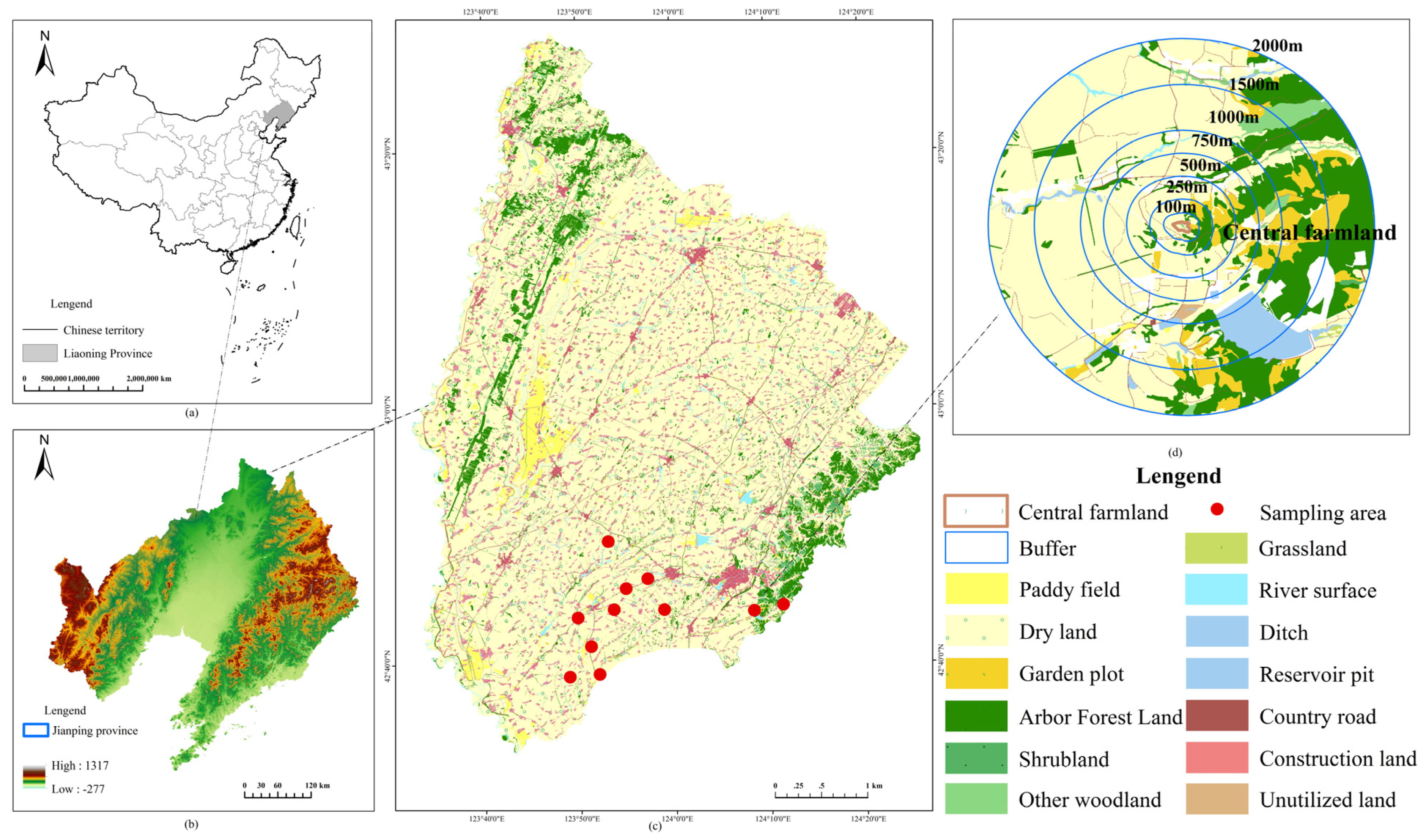
In this study, to make landscape design on the spatial scale related to arthropod species, we focused on the influence mechanism of landscape structure at different scales (landscape and habitat) on the diversity of epigaeic arthropods. More specifically, we propose the following research objectives: (1) On the landscape scale, we analyze the scale effect of the response of epigaeic arthropod diversity to landscape heterogeneity, and determine the optimal scale and minimum scale of the impact. (2) On the habitat scale, we predicted that: (i) the differences in epigaeic arthropod community structures in different habitat types were analyzed. (ii) The margin effect affects the distribution of epigaeic arthropods. (3) On the field scale, the vegetation structure of field margin strips was the main factor affecting the differences in epigaeic arthropods. (4) Clarify the landscape and environmental factors affecting epigaeic arthropods at two scales and construct the optimal model.

2. Materials and Methods

This study is carried out from three scales of landscape, habitat, and field, respectively, to explore the impact of landscape pattern, habitat type, and vegetation structure characteristics on epigaeic arthropod diversity, and to summarize the multi-scale effects of landscape structure on epigaeic arthropod diversity in the same area. At different scales, there are differences in the landscape structure affecting epigaeic arthropods, and the materials methods are also different.

2.1. Study Area

Changtu County is located in the south of Northeast China Plain (123°32′–124°26′ E, 42°3′–43°2′ N), with an administrative area of 4317 km2 and a total cultivated land area of 2667 km2 (Figure 1). It is a famous agricultural county in China. The county is dominated by an arable land system landscape, which is a typical dry farming area in the northern plain. It is the world’s “golden corn belt” and the largest peanut distribution center in Northeast China, which is also the significance of this study. The landform of the whole county transits from east to west from the hilly area to Liaohe plain area. The soil types mainly include dark brown soil, black soil, meadow soil, and aeolian sandy soil. The mangang plain in the central and southern part of the county is one of the key grain-producing areas in the county with a deep soil layer and developed agriculture. Changtu county belongs to the middle temperate humid monsoon continental climate, the average annual temperature is 7.0 °C, and the average annual rainfall is 607.5 mm [41]. Spring and autumn monsoon, long cold period, long crop growth cycle, and sparse natural vegetation. There are broad-leaved forest-based farmland shelterbelt systems and other non-crop habitats around farmland. Due to intensive farming methods, the homogenization of arable land system landscape is deepened and the sustainability of the agricultural system is reduced.

2.2. Biodiversity Sampling

In 2021, we selected 11 sampling areas to plant maize crops (Figure 2). According to the difference in habitat (2 orchards, 3 native grasslands, 3 other woodlands, 3 arbor woodlands) around cultivated land, it can be divided into 8 types of habitats: orchard, adjacent to an orchard, native grassland, adjacent to native grassland, other woodland, adjacent to other woodland, arbor forest land, adjacent to arbor forest land.
Epigaeic arthropods diversity sampling: the ‘five-point sampling method’ was used in the cultivated land. Three sampling points were set in the farmland margin and adjacent habitats, and three trap bottles (trap spacing greater than 10 m) were set at each sampling point, a total of 363 (0). Specific layout method: A 500 mL plastic cup with a bottom diameter of 5 cm, a top diameter of 10 cm, and a height of 12 cm was buried in the soil. The mouth of the cup was flat with the surface, and 150–200 mL ethylene glycol solution (20% concentration) and detergent (a drop) were poured into the cup. A plastic cover was installed above each trap and fixed with iron wire to play a protective role. After 6 days of trap placement, the captured epigaeic arthropods were stored in a PE bottle containing 75% alcohol until indoor identification. Vegetation diversity sampling: the farmland margin in the study area is mostly the transition zone between farmland and non-crop habitats. According to the different adjacent habitats of farmland, farmland margin can be divided into four types: farmland-orchard, farmland-native grassland, farmland-other woodland, and farmland-tree woodland. Six sampling plots of herb vegetation were randomly arranged around the trap of farmland margin in the sampling area. Considering the width of the vegetation zone (0.8–1.5 m) between the non-crop habitat and the farmland in the plot, as well as the composition and homogenization of herbaceous plants, we chose a plot of 0.5 × 0.5 m. The name, number of plants (clumps), average height (AH), and coverage (AC) of vegetation in the plots were recorded. In addition to directly reflecting biodiversity by the number of species (S), we use the Shannon diversity index (H) to reflect the number of species in a sample of a certain size. Differently, the Margalef richness index (Ma) reflects the chance of an individual appearing in a sample that includes all species in the community and was therefore chosen to characterize vegetation diversity. In addition, the species evenness index (E) is used to reflect the relative density of species in the sample, and to measure the proximity of different species in quantity. The diversity indices were calculated using PAST software [42]. The specific formula is as follows:
H = P i ln P i
E = H / ln S
M a = ( S 1 ) / ln N
Pi is the proportion of the number of individuals in group i, S is the number of species groups, and N is the total number of individuals.

2.3. Landscape Metrics

To comprehensively consider the impacts of land use (social attribute) and land cover (natural attribute), we reclassify the land use/cover in the study area into 10 first-level categories and 14 second-level categories based on the “LUCC classification system” (Appendix A). In particular, to reflect the degree of heterogeneity of the landscape, we selected 8 landscape structure indices: largest patch index (LPI), landscape shape index (LSI), Shannon’s diversity index (SHDI), patch richness density (PRD), contagion index (CONTAG), interspersion and juxtaposition index (IJI), landscape division index (DIVISION), aggregation index (AI). To obtain the landscape index, the land vector data of the study area is rasterized in ArcGIS 10. 2 (ESRI Geoinformatik, Hannover, Germany). The size of the particle is the key to effectively extracting information. We determine the optimal conversion particle size is 5 m, and Fragstats 4.2 software was used to calculate the concentric buffer (radius of 100, 250, 500, 750, 1000, and 1500 m) to describe the surrounding landscape indicators. The formulas used were as follows:
LPI = n m a x ( a i j ) j = 1 A ( 100 )
LSI = e i m i n e i
SHDI = i = 1 m [ P i ln ( P i ) ]
PRD = m / A
CONTAG = [ 1 + i = 1 m j = 1 n P i j ln ( P i j ) 2 ln ( m ) ] ( 100 )
IJI = i = 1 m k = i + 1 m [ ( e i k E ln e i k E ) ] ln ( m 1 ) ( 100 )
DIVISION = [ g i j m a x g i j ] ( 100 )
AI = [ g i j m a x g i j ] ( 100 )  
where, i and j are the number of patch types; m and n are the number of patch types; Pij is the probability that belongs to types i and j; aij is the area of a particular type of landscape; gij is the number of similar adjacent patches of corresponding landscape types, ei is the margin length of i element; A is the area of the whole landscape; N is the total number of patches in the landscape.

2.4. Statistical Analyses

Pearson correlation analysis was conducted between the diversity of farmland epigaeic arthropods and the landscape indices under different radii to analyze the impact of landscape variables on the diversity of farmland epigaeic arthropods at the landscape scale, and determine the optimal radius of this impact and the research scale of habitat scale. The index related to epigaeic arthropods is selected as the dependent variable, and the landscape index related to its obvious indigenousness is selected as the independent variable. Ridge regression analysis is used to solve the collinearity problem of independent variables in linear regression analysis. Then, the optimal model is selected according to the Akaike Information Criterion for small samples (AICc, the smaller the AICc value is, the better the model is).
Hierarchical clustering was used to analyze the similarity of epigaeic arthropod community structures in different habitats, which was completed in R software [43]. The effects of different habitats on the diversity of epigaeic arthropods were analyzed by one-way ANOVA. The linear regression model was constructed by selecting the epigaeic arthropod correlation index as the dependent variable and removing the linear herb vegetation structure factor as the independent variable. This analysis is completed by SPSS software. In addition, a Redundancy analysis (RDA) was used to explore the relationship between the structural factors of herb vegetation on farmland margin and the dominant species of common epigaeic arthropod species, and the two-dimensional ranking diagram of dominant and common species—key environmental factors were plotted. This analysis is calculated by CANOCO 5.

3. Results

We obtained the optimal radius at the landscape scale, the research scope at the habitat scale, and the characteristics of the plot scale itself, and analyzed the influence of environmental factors on epigaeic arthropods at various scales.

3.1. Arthropods and Plant Communities

We captured 9389 epigaeic arthropods, including 2148 in farmland, 4403 in the margin, and 2838 in non-crop habitats, belonging to 5 classes, 10 orders, 25 families, and 44 species (Appendix C). When individuals accounted for more than 20% of the total catch, it was considered the dominant group; when the proportion is 1–20%, it was considered the common group; when less than 1%, it was considered the rare group. The study captured mainly Gryllidae, accounting for 60% of the total, followed by Carabidae, accounting for 20% of the total. Formicidae, Theridiidae, and other three families constituted a common group. The remaining 18 families formed a rare group.
In terms of plant diversity, we collected 2569 herb plants, belonging to 3 classes, 21 orders, 21 families, and 42 species (Appendix B). Gramineae were mainly collected in this study, accounting for 44% of the total, followed by Asteraceae and Asterales, accounting for 18% and 10% of the total, respectively. Commelinaceae, Cyperaceae, Asclepiadaceae, and five other families formed a common group. The remaining 14 families formed a rare group.

3.2. Scale Responses of Epigaeic Arthropods Diversity on the Landscape Scale

There was no significant correlation between biodiversity index and landscape index at a 100 m radius (Table 1). At 1500 m radius, the correlation between the biodiversity index of epigaeic arthropods and the landscape index was the most significant. Species number (Sa) was negative correlated with LPI (p < 0.05) and CONTAG (p < 0.01), but positively correlated with IJI (p < 0.01), PRD (p < 0.05) and SHDI (p < 0.01). Shannon diversity index (Ha) was significantly positively correlated with PRD and SHDI (p < 0.05). Therefore, 100 m is the scale to study the diversity of epigaeic arthropods on the habitat scale. The 1500 m which the landscape index has the highest correlation with the biodiversity index, is the optimal radius to study the influence of landscape heterogeneity on epigaeic arthropod diversity on the landscape scale (Table 1).
Based on this, under the radius of 1500 m, the biodiversity index of epigaeic arthropods was used as the dependent variable, and the landscape index significantly related to it was used as the independent variable for ridge regression analysis, and the optimal model was selected according to the AICc value (Table 2). The species number (Sa) of epigaeic arthropods and five landscape indices including LPI, PRD, CONTAG, IJI, and SHDI, established 31 models, among which IJI and SHDI could explain the species number (S) of epigaeic arthropods at 76.7% level. The Shannon diversity index (Ha) of epigaeic arthropods and two landscape indices including PRD and SHDI were used to construct three models, among which PRD could explain the Shannon diversity (Ha) of epigaeic arthropods at 32% level.

3.3. Effects on Epigaeic Arthropods on the Habitat Scale

3.3.1. Effects of Habitat Types on Epigaeic Arthropods Community Structure

According to the hierarchical distance cluster analysis results (Figure 3), the eight types of habitats can be divided into two categories. The habitats adjacent to orchard farmland (HT1) and orchard (HT2) are one category, and the other types are another. The results showed that native grassland (HT4), shrubland (HT6), arbor forest land (HT8), and their adjacent farmlands had similar epigaeic arthropod community structure. The composition of epigaeic arthropods in farmlands adjacent to shrubland (HT5) was the closest to that in farmlands adjacent to arbor forest land (HT7), while the composition of epigaeic arthropods in farmlands adjacent to orchards (HT1) and orchards (HT2) was significantly different from that in other habitats.
The results of single factor analysis of variance (Table 3) showed that habitat types had significant effects on species number (Sa), Pielou evenness index (Ea), and individual number (N) of epigaeic arthropods (p < 0.05), but had no significant effect on Shannon diversity index (H). According to Figure 4, shrubland (HT6) had the most obvious effect on increasing the number of epigaeic arthropod individuals, and adjacent native grassland farmland (HT3) had the worst effect. The adjacent orchard farmland (HT1) had the largest number of epigaeic arthropod species (S), and the adjacent arbor forest farmland (HT7) had the smallest number. The distribution of epigaeic arthropods of the orchard (HT2) was the most uniform, and the evenness of (HT5) adjacent shrubland farmland was the smallest.

3.3.2. Margin Effect of Epigaeic Arthropods

The number of individuals and species (S) of epigaeic arthropods at the farmland margin of four types were significantly higher than those in adjacent farmland and non-crop habitats (Figure 5). In addition to the orchard type sample area, the Shannon diversity index (H) of epigaeic arthropods at the farmland margin was higher. For the different biodiversity indexes of epigaeic arthropods, the four types of farmland boundaries are shown as follows, the number of epigaeic arthropods: farmland–shrubland > farmland–arbor forest > farmland–native grassland > farmland–orchard; Shannon diversity index (H) of epigaeic arthropods: farmland land-orchard > farmland land-native grassland > farmland land-forest > farmland land-shrubland; species number of epigaeic arthropods (S): farmland land-shrubland > farmland land-arbor forest > farmland land-orchard > farmland land-native grassland; pielou evenness index (E): farmland land-orchard > farmland land-native grassland > farmland land-forest > farmland land-shrubland. Epigaeic arthropods have obvious margin effects. The field margin strips of the study area were the transition zone between non-crop habitat and farmland habitat. The herb vegetation structure was the main factor for this effect.

3.4. Effects of Epigaeic Arthropods on the Field Scale

3.4.1. Effects of Herb Vegetation Structure on Epigaeic Arthropod Diversity

To further understand the relationship between epigaeic arthropods and herb vegetation characteristic factors, we calculated Pearson’s correlation coefficients (Table 4). The Shannon diversity index of epigaeic arthropods (Hs) was significantly positively correlated with the Shannon diversity index (Hv), Average height (AH), Average cover (AC), and Margalef richness (Ma) of herb vegetation, while significantly negatively correlated with Pielou evenness (Ev). Pielou evenness (Es) of epigaeic arthropods was significantly positively correlated with species number (Sv) and Pielou evenness (Ev) of herb vegetation, while significantly negatively correlated with Average height (AH), Average cover (AC), and Margalef richness (Ma).
In addition, the variance expansion factor was used to test whether six characteristic variables which represent herb vegetation structure showed collinearity among groups. The results showed that there was collinearity between herb vegetation characteristic variables (Table 5). Stepwise linear regression was used to exclude variables that lead to multicollinearity. Finally, four variables are input into the linear regression model. Since the variance expansion factor (VIF) of all covariates in the model is less than 10, there is no multicollinearity problem in the modeling process.
The biodiversity index of epigaeic arthropods was used as the dependent variable, and the structural factors of herb vegetation related to its obvious indigenousness were used as independent variables for linear regression analysis, and the optimal model was screened according to the AICc value (Table 6). Epigaeic arthropod diversity (Hs), Pielou evenness (Es) herb vegetation Shannon diversity (Hv), average height (AH), coverage (AC), and Margalef richness (Ma) were constructed in 15 models, respectively. Hv and Ma can explain epigaeic arthropod Shannon diversity (Hs) at the level of 77.3%, and Hv, Ma, AC, and AH can explain Pielou evenness (Es) of epigaeic arthropod at the level of 97.2%.

3.4.2. Effects of Herb Vegetation Structure on Distribution of Epigaeic Arthropod Community

The sum of eigenvalues of the four axes of RDA is 0.8124, which cumulatively explains 100% of the species-environment relationship. Monte Carlo test shows that (First Axis, F = 16.8, P = 0.046; All Axis, F = 5.2, P = 0.042) can better explain the relationship between the herb vegetation structure on farmland margin and the distribution of epigaeic arthropod community. The results of partial RDA analysis (Table 7) showed that the effects of herb vegetation Shannon diversity (Hv) and Pielou evenness (Ev) on the distribution of epigaeic arthropod community reached the significant indigenous level (F = 6.5, P = 0.028, F = 30.5, P = 0.014), and the two explained 69.1% of the various number of epigaeic arthropod communities. RDA two-dimensional sort graph (Figure 6) with four explanatory variables was drawn.

4. Discussion

The arable land system can be interpreted as a heterogeneous region composed of habitat patches with certain biodiversity and intensive agricultural land, and the regional scope is the key. The interaction between species and environment at different scales is different, and the appropriate scale analysis is particularly important [35,44]. Studies have shown that landscape structure affects the dynamic evolution and species richness of complex populations on a large scale [21,45,46]. The analysis of plant and bird diversity in the agricultural landscape in Europe shows that landscape heterogeneity has a scale effect on biodiversity [3]. Species diversity has a strong scale dependence on landscape heterogeneity, due to the limited range of activities, the research on epigaeic arthropods is mostly on a small scale [47,48]. The studies on epigaeic arthropods at the habitat scale show that the implementation of compound planting pattern and other methods is conducive to the formation of microhabitats suitable for survival such as natural enemies (such as spiders, armor), and plays an important role in increasing biodiversity, especially natural enemy diversity. In addition to increasing crop diversity, on the field scale, the construction of adjacent non-crop habitats in farmland is the key to affecting natural enemy diversity and pest biological control in farmland [49,50]. Therefore, the diversity and community composition of epigaeic arthropods in arable land system landscapes are affected by different scale factors, and landscape reconstruction should be carried out from multiple scales.
In general, most of the current studies on agricultural biodiversity at home and abroad focused on large-scale sampling [51,52,53], while in small and medium-scale, different habitat types were used to distinguish and discuss [54,55]. How to combine margin characteristics, habitat types, and landscape structure to comprehensively discuss the landscape at different levels, which requires profound exploration and solution.
For studies aiming to describe the arable land system landscape structure, we propose metrics that reveal more information about connectivity, fragmentation, and diversity, such as contagion index, patch richness density, and Shannon’s diversity index, as they jointly reflect how a given matrix facilitates or hinders migration and re-colonization of habitat patches or remnants [56]. In this study, the relationship between the diversity of epigaeic arthropods and landscape structure in the northern plains was found at different landscape scales, which supported the previous study [57]. The smaller the degree of human disturbance, the higher the connectivity, the richer the patch types, the greater the number of epigaeic arthropod species, and the greater the Shannon diversity index. The higher the landscape heterogeneity, the richer the diversity of epigaeic arthropods.
Landscape attributes are significantly different with the different landscape scales concerned by the research. The larger the selected landscape scale is, the closer the landscape attributes are to the global common level. The smaller the selected landscape scale is, the more obvious the uniqueness of landscape attributes is [58]. Therefore, there is an optimal scale for the response of biodiversity to landscape structure at the landscape scale, but this scale is not unique. In the existing studies, Clough et al. considered that the radius range of 500 m was the appropriate scale to study the response of spiders to landscape structure [22], and there were also studies on the impact of landscape elements on the distribution of beetle diversity at the scale of about 1000 m [59]. In this study, when the radius is 100 m, the landscape elements have no significant impact on the diversity of epigaeic arthropods. Between 250 m and 1500 m, with the increase of radius, the correlation between each landscape index and biodiversity index increased as a whole, and the correlation was the most obvious at 1500 m, and the correlation decreased at 2000 m. Therefore, we believe that 1500 m is the optimal scale of landscape elements affecting the diversity of epigaeic arthropods. Multi-scale studies are conducive to eliminating misjudgments under general rules, so as to comprehensively evaluate species diversity and find appropriate scales for biodiversity conservation [60,61].
In terms of which scale should be used in future works that address how landscape features affect epigaeic arthropods (e.g., [62,63,64]), we found an optimal scale for the landscape scale. For the habitat scale, domestic and foreign scholars have done a lot of research on the impact of different habitats on epigaeic arthropods, mainly concentrating on the natural, semi-natural, and artificial three habitat types, and discussed the impact of different habitat types on the diversity of epigaeic arthropods [65,66,67]. A large number of studies have found that different land use types have different impacts on soil fauna communities, especially the distribution characteristics of dominant groups and common groups in various land-use types [68,69].
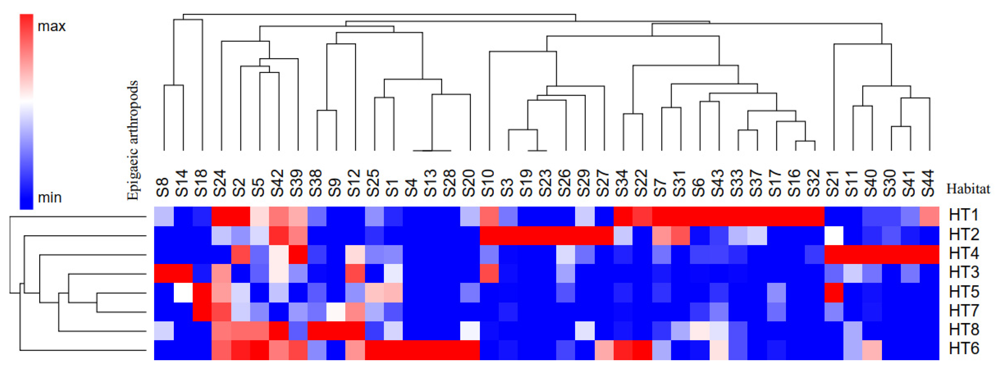
This is further complemented in our study, for example, according to the distribution characteristics of habitat classification, Harpalus sinicus, Pheropsophus occiptalis, Holotrichia oblita Faldermann, Chrysacris liaoningensis, etc., as the same category, mainly distributed in the orchard. Non-crop habitats have more epigaeic arthropod diversity [70] due to their own vegetation conditions and less human disturbance, namely margin effects. At the same time, the spillover effect also affects the diversity of epigaeic arthropods in the surrounding farmland habitats. We concluded that the community structure of epigaeic arthropods in grassland, shrubland, arbor land, and their adjacent farmland habitats in the arable land system landscape of the plain area was similar.
As a way of spatial connection of different types of habitats, the margin is of great significance in the ecological process, and its community groups and the overall number are higher than those of adjacent habitats, namely the margin effect [37,71]. Margin not only contains the characteristics and components of adjacent habitats, but also forms more environmental characteristics that are not included in adjacent habitats according to their characteristics, resulting in more functions and characteristics [72]. In this study, the number of individuals and species (S) of epigaeic arthropods at the margin of four types of non-crop-farmland habitats (orchard, shrub land, arbor forest land, and grassland) were significantly higher than those of adjacent farmland and other non-tillage habitats, and the margin effect was significant. The study area benefited from the three-north shelter forest system in northern China. Previous studies focused on the impact of farmland shelter forests on biodiversity or arable land yield. Constrained by the inherent thinking of local farmers, herbaceous plant clumps separated from farmland management (fertilization, pesticides, etc.) are considered negative factors of the agricultural ecosystem. This study provides a new idea for farmers to implement farmland management measures on the habitat scale.
Vegetation structure in non-crop habitats, as a major habitat control factor, is considered to be an environmental variable affecting biodiversity and ecosystem services in farmland [73,74,75]. Garratt et al. argued that complex and continuous understory vegetation can significantly improve the diversity of pollinators and natural enemy groups of epigaeic arthropods in farmland [71]. Tougeron et al. believed that at the habitat scale, the margin type or the distance to the margin affected the activity density and parasitic rate of beetles and spiders [3]. On the habitat scale, we found that there was a significant relationship between the distribution of epigaeic arthropod community and the vegetation structure through the redundancy analysis (RDA). The Shannon diversity and Pielou evenness of herb vegetation were important factors affecting the composition of the epigaeic arthropod community. The composition of heterogeneous herb vegetation structure can often provide diversified microhabitats for a variety of taxonomic groups, thus providing a broader niche for the habitat survival of more organisms [61,76,77]. In addition, due to the weak migration ability of most epigaeic arthropods, it is necessary to strengthen the protection of habitat scale, especially the restoration and protection of plant diversity in habitat, so as to play a positive role in improving the biodiversity of epigaeic arthropod communities in arable land system landscape to a certain extent.
In the main grain-producing areas of northern China, the plain area represented by Changtu County in the study area undertakes the important task of ensuring regional and even national food security. Agricultural production is characterized by a small number of planting plants and livestock species to replace the natural state of biodiversity, resulting in a wide range of environmental structure that tends to simplify and single [78,79]. In addition, due to China’s relevant policies, the farmland management measures implemented by farmers are limited to the arable land they own, which makes the management of arable land a single scale and lacks systematicness and integrity. Our research results clarify the key points of cropland system protection at multiple scales, and provide a detailed reference for the implementation of policies related to the sustainable development of cropland systems in northern China in the future. Optimizing arable land system landscape structure and enhancing landscape heterogeneity are effective ways to protect biodiversity and ecosystem services [80]. Of course, there is no “one-size-fits-all” answer to the preservation of agricultural biodiversity. The appropriate scale is the optimal lever for the protection of agricultural biodiversity, which promotes the accurate implementation of agricultural management measures at different scales. Combined with the macro layout at the landscape scale and the dynamic adjustment at the habitat scale, the overall landscape layout, and microenvironment control can be used to maintain regional agricultural biodiversity and enhance the sustainability of the agricultural system, so as to improve the agricultural ecological environment and ensure the safety of the food system.
In the future, this study can classify and discuss epigaeic arthropods, and further clarify the interaction between different functional groups at different scales. In addition, climate, soil, and other environmental variables can also be introduced to make a more comprehensive discussion of other regions. In addition, this study chose to obtain biodiversity data during the crop maturity period (September). In future research, data from other seasons can be combined to enhance the broad applicability of the research conclusions.

5. Conclusions

Discussing the response of epigaeic arthropod diversity to environmental changes at multiple spatial scales in detail is essential for the sustainable development of the arable land system in the context of global change and biodiversity crisis. Based on landscape data and biodiversity data, from the perspective of biodiversity conservation, we used scale leverage (landscape, habitat, and field) to clarify the direction of efficient implemen-tation of agricultural system management measures in the northern plains of China.
We conclude that at the landscape scale, the landscape structure has a significant scale effect on the diversity of epigaeic arthropods, and 1500 m is the optimal radius for improving the biodiversity level by optimizing the landscape structure. On this scale, the largest patch index, patch richness density, contagion index, interspersion and juxtaposi-tion index, and Shannon diversity index significantly affected the biodiversity of epigaeic arthropods. The greater the landscape heterogeneity, the higher the level of epigaeic ar-thropod diversity. This result can point out the direction for the large-scale changes in landscape patterns in the study area. 100 m radius is the habitat scale to explore the factors affecting the diversity of epigaeic arthropods. On this scale, habitat types affect the diver-sity of epigaeic arthropods, and have a significant impact on the abundance and commu-nity structure richness of epigaeic arthropods, as well as the relative density between spe-cies. The number of epigaeic arthropods in the shrubland is the most abundant, the farmland adjacent to the orchard has the largest number of species, and the number of epigaeic arthropods of different species in the orchard is more evenly distributed. The rational layout of non-crop habitat patches and farmland is an effective way to protect the diversity of epigaeic arthropods at the field scale. To some extent, our study showed that field margin strips should be the unique cornerstones of agro-ecological landscape design strategies on this scale. The species and quantity distribution of epigaeic arthropods have obvious margin effects, and the herb vegetation structure of farmland margin is the main influencing factor for this effect. On the field scale, Shannon diversity, Pielou even-ness, average height, average cover, and Margalef richness of herb vegetation are important environmental factors affecting the diversity and community structure of epigaeic arthro-pods.
Biodiversity is the basis for a sustainable arable land system. Our findings underscore that, in agricultural landscapes dominated by arable land, combining precise implementation at various scales with comprehensive coordination at multiple scales has greater potential to support regional biodiversity than focusing on a single scale. We believe that using spatial scales to protect biodiversity is consistent with the reality of agricultural management, which is of great significance to the rational distribution of the arable land system.

Author Contributions

Conceptualization, Z.B.; methodology, Y.Y; software, Y.Y. and Y.Z.; validation, S.W.; formal analysis, Y.Y. and Y.Z.; investigation, Y.Y. and Y.Z.; resources, Y.Y.; data curation, Y.Z.; writing—original draft preparation, Y.Z.; writing—review and editing, Z.B. and Y.Z.; visualization, Y.Y. and Y.Z.; supervision, S.W.; project administration, Z.B.; funding acquisition, Z.B. All authors have read and agreed to the published version of the manuscript.

Funding

This research was funded by Natural Science Foundation of Liaoning Province (Grant No. 2019-ZD-0709).

Institutional Review Board Statement

Not applicable.

Informed Consent Statement

Not applicable.

Data Availability Statement

The data used to support the findings of this study are available from the corresponding author upon request.

Acknowledgments

Thank you to the reviewers for their valuable feedback on the manuscript. Thank you to the team members for their hard work in field sampling.

Conflicts of Interest

The authors declare no conflict of interest.

Appendix A

Table A1. Land use and cover type division in Changtu County.
Serial NumberLevel 1 TypeSerial NumberLevel 2 Type
01Cultivated land011Paddy field
012Dry land
02Garden plot020Garden plot
03Forest031Arbor Forest Land
032Shrubland
033Other woodland
04Grassland040Grassland
05River and canal051River surface
052Ditch
06Reservoir pit060Reservoir pit
07Tidal flat070Tidal flat
08Country road080Country road
09Construction land090Construction land
10Unutilized land100Unutilized land

Appendix B

Table A2. Statistical table of herb vegetation.
Herb VegetationLatin Names
Monocots Oales SmallPoaceae BarnhartEleusine indica (L.) Gaertn.
Digitaria sanguinalis (L.) Scop.
Cynodon dactylon (L.) Pers.
Echinochloa crus-galli (L.) P. Beauv
Etaria viridis (L.) Beauv.
FarinosaeSubordo CommelinineaeCommelina communis L.
CyperalesCyperaceae Juss.Cyperaceae
Cyperusrotundus L.
Dicotyledoneae EuphorbialesEuphorbiaceae Juss.Acalypha australis L.
CampanulalesAsteraceae Bercht. & J. PreslCirsium japonicum Fisch. ex DC.
Ixeris polycephala Cass.
Erigeron canadensis L.
Artemisia caruifolia Buch.-Ham. ex Roxb
Ambrosia artemisiifolia L.
Aster tataricus L. f.
Xanthium sibiricum Patrin ex Widder
Artemisia mongolica (Fisch. ex Bess.) Nakai
Ambrosia trifida L.
Siegesbeckia orientalis L.
Chrysanthemum indicum L.
ContortaeAsclepiadaceaeMetaplexis japonica (Thunb.) Makino
Rosales Bercht. & J. PreslLeguminosaeSesbania cannabina (Retz.) Poir.
ubiflorae ConvolvulaceaeConvolvulus arvensis L.
Asterales Link Asteraceae Bercht. & J. PreslBidens pilosa L.
Artemisia argyi Lévl. et Van.
Urticales Moraceae Gaudich.Humulus scandens (Lour.) Merr.
entrospermae ChenopodiaceaeDysphania ambrosioides (Linnaeus) Mosyakin & Clemants
Kochia scoparia (L.) Schrad.
Polygonales PolygonaceaePolygonum perfoliatum L.
Polygonum aviculare L.
Rumexacetosa L.
Lamiales Bromhead Lamiaceae MartinovLeonurus japonicus Houtt
Lagopsis supina (Steph. ex Willd.) Ik.-Gal. ex Knorr.
Santalales R. Br. Santalaceae R. Br.Thesium chinense Turcz.
Malvales Juss. Malvaceae Juss.Abutilon theophrasti Medicus
Geraniales Juss. Geraniaceae Juss.Geranium wilfordii Maxim.
Apiales Nakai Apiaceae Lindl.Cnidium monnieri (L.) Cuss.
ParietalesViolaceae Batsch Viola hamiltoniana D.Don
Asterales Link Asteraceae Bercht. & J. PreslCirsium setosum
Artemisiaselengensis Turcz.
Caryophyllales ChenopodiaceaeChenopodium album L.
Sphenopsida Equisetales Equisetaceae Michx. ex DC.Equisetum arvense L.

Appendix C

Table A3. Statistical table of epigaeic arthropod types and numbers in different habitats.
Epigaeic ArthropodsNumber (Families)Latin NamesNumber (Specie)
InsectaColeopteraCarabidaeSP1Chlaenius micansS1
Harpalus pallidipennisS2
Harpalus sinicusS3
Calosoma maximovicziS4
Dolichus halensisS5
Harpalus rubefactusS6
Harpalus griseusS7
Chlaenius praefectusS8
Chlaenius junceusS9
Pheropsophus occipitalisS10
Lachnolebia cribricollisS11
Harpalus calceatusS12
Callida splendidulaS13
HydrophiloideaSP2Laccobius inopinusS14
StaphylinidaeSP3Pinophilus punctatissimusS15
Scydmaeninae OligotaS16
TenebrionindaeSP4Opatrum subaratumS17
Gonocephalum reticulatumS18
MelolonthidaeSP5Holotrichia oblitaS19
Trematodes tenebrioides PallasS20
ChrysomelidaeSP6Monolepta hieroglyphicaS21
shining leafchaferSP7Anomala aulax WiedemannS22
CetoniidaeSP8Oxycetonia jucunda FaldermannS23
OrthopteraGryllidaeSP9Teleogryllus emmaS24
Loxoblemmus doenitziSteinS25
AcrididaeSP10HaplofropisS26
Chrysacris liaoningensisS27
CatantopidaeSP11Calliptamus abbreviatus IkonnS28
Shirakiacris shirakiiS29
PyrgomorphidaeSP12Atractomorpha sinensis BolvarS30
GryllotalpidaeSP13Gryllotalpa sppsS31
DersmapteraLabiduridaeSP14Earwig FurficulidaeS32
HymenopteraFormicidaeSP15Camponotus japonicusS33
Formica japonicaS34
HemipteraNepidaeSP16Ranatra chinensis MayrtS35
AradidaeSP17flat bugS36
CoreidaeSP18Corizus albomarginatus BlöteS37
ArachnoideaOpilionesPhalangiidaeSP19 S38
AraneaeAgelenidaeSP20 S39
TheridiidaeSP21 S40
DiplopodaPolydesmidaParadoxosomatidaeSP22Asiomorpha coarctataS41
StrongylosomidaeSP23Prospirobolus joannsiS42
MyriapodaGeophilomorphaScolopendridaeSP24Scolopendra mutilansS43
MalacostracaIsopodaOnsicidaeSP25Armadillidium vulgareS44
Note: Identification of epigaeic arthropods to the species level (spiders identified to families level) used Zeiss stereomicroscope (ZEIS: Stemi 2000-C).

References

  1. Fahrig, L.; Girard, J.; Duro, D.; Pasher, J.; Smith, A.; Javorek, S.; King, D.; Lindsay, K.F.; Mitchell, S.; Tischendorf, L. Farmlands with smaller crop fields have higher within-field biodiversity. Agric. Ecosyst. Environ. 2015, 200, 219–234. [Google Scholar] [CrossRef]
  2. Gurgel, A.C.; Reilly, J.; Blanc, E. Agriculture and forest land use change in the continental United States: Are there tipping points? iScience 2021, 24, 102772. [Google Scholar] [CrossRef] [PubMed]
  3. Tougeron, K.; Couthouis, E.; Marrec, R.; Barascou, L.; Baudry, J.; Boussard, H.; Burel, F.; Couty, A.; Doury, G.; Francis, C.; et al. Multi-scale approach to biodiversity proxies of biological control service in European farmlands. Sci. Total Environ. 2022, 822, 153569. [Google Scholar] [CrossRef] [PubMed]
  4. Badenhausser, I.; Gross, N.; Mornet, V.; Roncoroni, M.; Saintilan, A.; Rusch, A. Increasing amount and quality of green infrastructures at different scales promotes biological control in agricultural landscapes. Agric. Ecosyst. Environ. 2020, 290, 106735. [Google Scholar] [CrossRef]
  5. Galpern, P.; Vickruck, J.; Devries, J.H.; Gavin, M.P. Landscape complexity is associated with crop yields across a large temperate grassland region. Agric. Ecosyst. Environ. 2020, 290, 106724. [Google Scholar] [CrossRef]
  6. Haan, N.L.; Zhang, Y.; Landis, D.A. Predicting landscape configuration effects on agricultural pest suppression. Trends Ecol. Evol. 2020, 35, 175–186. [Google Scholar] [CrossRef] [Green Version]
  7. Thomine, E.; Mumford, J.; Rusch, A.; Desneux, N. Using crop diversity to lower pesticide use: Socio-ecological approaches. Sci. Total Environ. 2021, 804, 150156. [Google Scholar] [CrossRef]
  8. Newbold, T.; Hudson, L.N.; Hill, S.L.; Contu, S.; Lysenko, I.; Senior, R.A.; Börger, L.; Bennett, D.J.; Choimes, A.; Collen, B.; et al. Global effects of land use on local terrestrial biodiversity. Nature 2015, 520, 45–50. [Google Scholar] [CrossRef] [Green Version]
  9. Delabre, I.; Rodriguez, L.O.; Smallwood, J.M.; Scharlemann, J.P.W.; Alcamo, J.; Antonarakis, A.S.; Rowhani, P.; Hazell, R.J.; Aksnes, D.L.; Balvanera, P.; et al. Actions on sustainable food production and consumption for the post-2020 global biodiversity framework. Sci. Adv. 2021, 7, eabc8259. [Google Scholar] [CrossRef]
  10. Kirwan, L.; Connolly, J.; Finn, J.A.; Brophy, C.; Lüscher, A.; Nyfeler, D.; Sebastià, M.-T. Diversity–interaction modeling: Estimating contributions of species identities and interactions to ecosystem function. Ecology 2009, 90, 2032–2038. [Google Scholar] [CrossRef]
  11. Haan, N.L.; Iuliano, B.G.; Gratton, C.; Landis, D.A. Designing agricultural landscapes for arthropod-based ecosystem services in North America. Adv. Ecol. Res. 2021, 64, 191–250. [Google Scholar] [CrossRef]
  12. Aviron, S.; Lalechère, E.; Duflot, R.; Parisey, N.; Poggi, S. Connectivity of cropped vs. semi-natural habitats mediates biodiversity: A case study of carabid beetles communities. Agric. Ecosyst. Environ. 2018, 268, 34–43. [Google Scholar] [CrossRef]
  13. Torma, A.; Gallé, R.; Bozsó, M. Effects of habitat and landscape characteristics on the arthropod assemblages (Araneae, Orthoptera, Heteroptera) of sand grassland remnants in Southern Hungary. Agric. Ecosyst. Environ. 2014, 196, 42–50. [Google Scholar] [CrossRef]
  14. Albrecht, M.; Williams, N.M.; Tschumi, M. The effectiveness offlower strips and hedgerows on pest control, pollination services and crop yield: A quantitative synthesis. Ecol. Lett. 2020, 11, 1488–1498. [Google Scholar] [CrossRef]
  15. Bosch-Serra, À.D.; Padró, R.; Boixadera-Bosch, R.R.; Orobitg, J.; Yagüe, M.R. Tillage and slurry over-fertilization affect oribatid mite communities in a semiarid mediterranean environment. Appl. Soil Ecol. 2014, 84, 124–139. [Google Scholar] [CrossRef] [Green Version]
  16. Tscharntke, T.; Klein, A.M.; Kruess, A.; Dewenter, I.; Thies, C. Landscape perspectives on agricultural intensification and biodiversity-ecosystem service management. Ecol. Lett. 2005, 8, 857–874. [Google Scholar] [CrossRef]
  17. Fahrig, L.; Baudry, J.; Brotons, L.; Burel, F.G.; Crist, T.O.; Fuller, R.J.; Sirami, C.; Siriwardena, G.M.; Martin, J. Functional landscape heterogeneity and animal iodiversity in agricultural landscapes. Ecol. Lett. 2011, 14, 101–112. [Google Scholar] [CrossRef]
  18. Holland, J.M.; Storkey, J.; Lutman, P.J.W.; Birkett, T.C. Utilisation of agri-environment scheme habitats to enhance invertebrate ecosystem service providers. Agric. Ecosyst. Environ. 2014, 183, 103–109. [Google Scholar] [CrossRef]
  19. Muneret, L.; Mitchell, M.; Seufert, V.; Aviron, S.; Djoudi, E.A.; Pétillon, J.; Plantegenest, M.; Thiéry, D.; Rusch, A. Evidence that organic farming promotes pest control. Nat. Sustain. 2018, 1, 361–368. [Google Scholar] [CrossRef]
  20. Jonsson, M.; Straub, C.S.; Didham, R.K.; Buckley, H.L.; Case, B.S.; Hale, R.J.; Gratton, C.; Wratten, S.D. Experimental evidence that the effectiveness of conservation biological control depends on landscape complexity. J. Appl. Ecol. 2015, 52, 1274–1282. [Google Scholar] [CrossRef]
  21. Larsen, A.E.; Noack, F. Impact of local and landscape complexity on the stability of field-level pest control. Nat. Sustain. 2020, 4, 120–128. [Google Scholar] [CrossRef]
  22. Clough, Y.; Kruess, A.; Kleijn, D.; Tscharntke, T. Spider diversity in cereal fields: Comparing factors at local, landscape and regional scales. J. Biogeogr. 2005, 32, 2007–2014. [Google Scholar] [CrossRef]
  23. Schmidt, M.H.; Tscharntke, T. The role of perennial habitats for Central European farmland spiders. Agric. Ecosyst. Environ. 2005, 105, 235–242. [Google Scholar] [CrossRef]
  24. Liu, Y.M.; Lu, X.L.; Ding, S.Y.; Zhou, L.Y.; Zhang, C.C. Distribution pattern of pollination community under different agricultural landscape context. Acta Ecol. Sin. 2020, 40, 2376–2385. [Google Scholar] [CrossRef]
  25. Navarro, L.M.; Fernández, N.; Guerra, C.; Guralnick, R.; Kissling, W.D.; Londoño, M.C.; Muller-Karger, F.; Turak, E.; Balvanera, P.; Costello, M.J.; et al. Monitoring biodiversity change through effective global coordination. Curr. Opin. Environ. Sustain. 2017, 29, 158–169. [Google Scholar] [CrossRef]
  26. Martel, G.; Aviron, S.; Joannon, A.; Lalechère, E.; Roche, B.; Boussard, H. Impact of farming systems on agricultural landscapes and biodiversity: From plot to farm and landscape scales. Eur. J. Agron. 2019, 107, 53–62. [Google Scholar] [CrossRef]
  27. Bianchi, F.J.J.; Booij, C.J.H.; Tscharntke, T. Sustainable pest regulation in agricultural landscapes: A review on landscape composition, biodiversity and natural pest control. Proc. R. Soc. B Biol. Sci. 2006, 273, 1715–1727. [Google Scholar] [CrossRef] [Green Version]
  28. Chaplin-Kramer, R.; O’Rourke, M.E.; Blitzer, E.J.; Kremen, C. A meta-analysis of crop pest and natural enemy response to landscape complexity: Pest and natural enemy response to landscape complexity. Ecol. Lett. 2011, 14, 922–932. [Google Scholar] [CrossRef]
  29. Rosenfield, M.F.; Brown, L.M.; Anand, M. Increasing cover of natural areas at smaller scales can improve the provision of biodiversity and ecosystem services in agroecological mosaic landscapes. J. Environ. Manag. 2022, 303, 114248. [Google Scholar] [CrossRef]
  30. Aviron, S.; Burel, F.; Baudry, J.; Schermann, N. Carabid assemblages in agricultural landscapes: Impacts of habitat features, landscape context at different spatial scales and farming intensity. Agric. Ecosyst. Environ. 2005, 108, 205–217. [Google Scholar] [CrossRef]
  31. Li, Y.; Dong, S.; Liu, S.; Su, X.; Wang, X.; Zhang, Y.; Zhao, Z.; Gao, X.; Li, S.; Tang, L. Relationships between plant diversity and biomass production of alpine grasslands are dependent on the spatial scale and the dimension of biodiversity. Ecol. Eng. 2018, 127, 375–382. [Google Scholar] [CrossRef]
  32. Gabriel, D.; Thies, C.; Tscharntke, T. Local diversity of arable weeds increases with landscape complexity. Perspect. Plant. Ecol. 2005, 7, 85–93. [Google Scholar] [CrossRef]
  33. Maisonhaute, J.; Peres-Neto, P.; Lucas, É. Influence of agronomic practices, local environment and landscape structure on predatory beetle assemblage. Agric. Ecosyst. Environ. 2010, 139, 500–507. [Google Scholar] [CrossRef]
  34. Bian, Z.X.; Zhang, Y.F.; Yang, Y.B.; Yu, M. The effect of agricultural landscape structure on the qualitative food web structure of corn pests and predatory natural enemies. Chin. J. Eco-Agric. 2020, 28, 1475–1487. [Google Scholar] [CrossRef]
  35. Tscharntke, T.; Brandl, R. Plant-insect interactions in fragmented landscapes. Annu. Rev. Entomol. 2004, 49, 405–430. [Google Scholar] [CrossRef] [PubMed]
  36. Pardon, P.; Reheul, D.; Mertens, J.; Reubens, B.; De Frenne, P.; De Smedt, P.; Proesmans, W.; Van Vooren, L.; Verheyen, K. Gradients in abundance and diversity of ground-dwelling arthropods as a function of distance to tree rows in temperate arable agroforestry systems. Agric. Ecosyst. Environ. 2019, 270–271, 114–128. [Google Scholar] [CrossRef]
  37. Tscharntke, T.; Bommarco, R.; Clough, Y.; Crist, T.O.; Kleijn, D.; Rand, T.A.; Tylianakis, J.M.; Nouhuys, S.V.; Vidali, S. Conservation biological control and enemy diversity on a landscape scale. Biol. Control. 2007, 43, 294–309. [Google Scholar] [CrossRef]
  38. Hawksworth, D.L.; Bull, A.T.; Caruso, T.; Pigino, G.; Migliorini, M. The Berger-Parker index as an effective tool for monitoring the biodiversity of disturbed soils: A case study on Mediterranean oribatid (Acari; Oribatida) assemblagea. Biodivers. Conserv. 2007, 16, 3277–3285. [Google Scholar] [CrossRef]
  39. Djoudi, E.A.; Marie, A.; Mangenot, A.; Puech, C.; Aviron, S.; Plantegenest, M.; Pétillon, J. Farming system and landscape characteristics differentially affect two dominant taxa of predatory arthropods. Agric. Ecosyst. Environ. 2018, 259, 98–110. [Google Scholar] [CrossRef]
  40. Heij, S.E.D.; Willenborg, C.J. Connected carabids: Network interactions and their impact on biocontrol by carabid beetles. Bioscience 2020, 70, 490–500. [Google Scholar] [CrossRef]
  41. Guo, X.; Bian, Z.X.; Wang, S.; Wang, Q.B.; Zhang, Y.F.; Zhou, J.; Yu, M. Prediction of the spatial distribution of soil arthropods using a random forest model: A case study in Changtu County, Northeast China. Agric. Ecosyst. Environ. 2020, 292, 106818. [Google Scholar] [CrossRef]
  42. Hammer, Ø.; Harper, D.A.T.; Ryan, P.D. PAST: Palacontological Statistics software package for education and data analysis. Palaeontol. Electron. 2001, 4, 4–9. Available online: https://palaeo-electronica.org/2001_1/past/issue1_01.htm (accessed on 1 March 2022).
  43. RStudio Team. RStudio: Integrated Development for R; RStudio, PBC: Boston, MA, USA, 2020; Available online: http://www.rstudio.com (accessed on 15 March 2022).
  44. Bosem, A.B.; Tscharntke, T.; Clough, Y.; Batáry, P. Landscape-scale interactions of spatial and temporal cropland heterogeneity drive biological control of cereal aphids. J. Appl. Ecol. 2017, 54, 1804–1813. [Google Scholar] [CrossRef] [Green Version]
  45. Benton, T.G.; Vickery, J.A.; Wilson, J.D. Farmland biodiversity: Is habitat heterogeneity the key? Trends Ecol. Evol. 2003, 18, 182–188. [Google Scholar] [CrossRef]
  46. Gurr, G.M.; Wratten, S.D.; Landis, D.A.; You, M. Habitat management to suppress pest populations: Progress and prospects. Annu. Rev. Entomol. 2017, 62, 91–109. [Google Scholar] [CrossRef] [PubMed]
  47. Schindler, S.; Wehrden, H.V.; Poirazidis, K.; Wrbka, T.; Kati, V. Multiscale performance of landscape metrics as indicators of species richness of plants, insects and vertebrates. Ecol. Indic. 2013, 31, 41–48. [Google Scholar] [CrossRef]
  48. Sarthou, J.-P.; Badoz, A.; Vaissière, B.; Chevallier, A.; Rusch, A. Local more than landscape parameters structure natural enemy communities during their overwintering in semi-natural habitats. Agric. Ecosyst. Environ. 2014, 194, 17–28. [Google Scholar] [CrossRef]
  49. Landis, D.A.; Wratten, S.D.; Gurr, G.M. Habitat management to conserve natural enemies of arthropod pests in agriculture. Annu. Rev. Entomol. 2000, 45, 175–201. [Google Scholar] [CrossRef]
  50. Montgomery, I.; Caruso, T.; Reid, N. Hedgerows as ecosystems: Service delivery, management, and restoration. Annu. Rev. Ecol. Evol. Syst. 2020, 51, 012120–100346. [Google Scholar] [CrossRef]
  51. Kolozsvary, M.B.; Swihart, R.K. Habitat fragmentation and the distribution of amphibians: Patch and landscape correlates in farmland. Can. J. Zool. 1999, 77, 1288–1299. [Google Scholar] [CrossRef]
  52. Kleijn, D.; Verbeek, M. Factors affecting the species richness of arable field boundary vegetation. J. Appl. Ecol. 2000, 37, 256–266. [Google Scholar] [CrossRef]
  53. Peng, Y.; Qing, F.T.; Mi, K.; Xue, D.Y. Study progress on spatial scale effects and coupling relationships of different levels in biodiversity. Acta Ecol. Sin. 2013, 35, 577–583. [Google Scholar] [CrossRef]
  54. Vannier, C.; Vasseur, C.; Hubert-Moy, L.; Baudry, J. Multiscale ecological assessment of remote sensing images. Landsc. Ecol. 2011, 26, 1053–1069. [Google Scholar] [CrossRef]
  55. Loureiro, A.M.; Nams, V.O.; White, S.N.; Cutler, G.C. Short-term dispersal and long-term spatial and temporal patterns of carabidae (Coleoptera) in lowbush blueberry fields. Environ. Entomol. 2020, 49, 572–579. [Google Scholar] [CrossRef]
  56. Hoffmann, H.; Peter, F.; Herrmann, J.D.; Donath, T.W.; Diekötter, T. Benefits of wildflower areas as overwintering habitats for ground-dwelling arthropods depend on landscape structural complexity. Agric. Ecosyst. Environ. 2021, 314, 107421. [Google Scholar] [CrossRef]
  57. Riitters, K.; Vogt, P.; Soille, P.; Estreguil, C. Landscape structures from mathematical morphology on maps with contagion. Landsc. Ecol. 2009, 24, 699–709. [Google Scholar] [CrossRef]
  58. Pasher, J.; Mitchell, S.W.; King, D.J.; Fahrig, L.; Smith, A.C.; Lindsay, K.E. Optimizing landscape selection for estimating relative effects of landscape variables on ecological responses. Landsc. Ecol. 2000, 28, 371–383. [Google Scholar] [CrossRef]
  59. Zhao, Z.H.; Wang, Y.; He, D.H.; Guan, X.Q.; Xin, M. Responses of wheat aphids and parasitic wasps to agricultural landscape structures and analysis of key landscape factors. Acta Ecol. Sin. 2012, 32, 472–482. [Google Scholar] [CrossRef]
  60. Jackson, H.B.; Fahrig, L. Are ecologists conducting research at the optimal scale? Glob. Ecol. Biogeogr. 2015, 24, 52–63. [Google Scholar] [CrossRef]
  61. Wilson, M.C.; Hu, G.; Jiang, L.; Liu, J.; Jin, Y.; Yu, M.; Wu, J. Assessing habitat fragmentation’s hierarchical effects on species diversity at multiple scales: The case of Thousand Island Lake, China. Landsc. Ecol. 2020, 35, 501–512. [Google Scholar] [CrossRef]
  62. Mendes, E.S.; Fonseca, C.; Marques, S.F.; Maia, D.; Ramos Pereira, M.J. Bat richness and activity in heterogeneous landscapes: Guild-specific and scale-dependent? Landsc. Ecol. 2017, 32, 295–311. [Google Scholar] [CrossRef]
  63. Happe, A.; Riesch, F.; Rösch, V.; Gallé, R.; Tscharntke, T.; Batáry, P. Small-scale agricultural landscapes and organic management support wild bee communities of cereal field boundaries. Agric. Ecosyst. Environ. 2018, 254, 92–98. [Google Scholar] [CrossRef] [Green Version]
  64. Emery, S.E.; Jonsson, M.; Silva, H.; Ribeiro, A.; Mills, N.J. High agricultural intensity at the landscape scale benefits pests, but low intensity practices at the local scale can mitigate these effects. Agric. Ecosyst. Environ. 2021, 306, 107199. [Google Scholar] [CrossRef]
  65. Pfiffner, L.; Luka, H. Overwintering of arthropods in soils of arable fields and adjacent semi-natural habitats. Agric. Ecosyst. Environ. 2000, 78, 215–222. [Google Scholar] [CrossRef]
  66. Knapp, M.; Řezáč, M. Even the smallest non-crop habitat islands could be beneficial: Distribution of carabid beetles and spiders in agricultural landscape. PLoS ONE 2015, 10, 0123052. [Google Scholar] [CrossRef] [PubMed]
  67. Harlio, A.; Kuussaari, M.; Heikkinen, R.K.; Arponen, A. Incorporating landscape heterogeneity into multi-objective spatial planning improves biodiversity conservation of semi-natural grasslands. J. Nat. Conserv. 2019, 49, 37–44. [Google Scholar] [CrossRef]
  68. Ferraro, D.O.; Ghersa, C.M. Exploring the natural and human-induced effects on the assemblage of soil microarthropod communities in Argentina. Eur. J. Soil. Biol. 2007, 43, 109–119. [Google Scholar] [CrossRef]
  69. Mmor, M.; Cianciolo, J. Diversity of soil mites along a gradient of land use types in New York. Appl. Soil Ecol. 2007, 35, 140–153. [Google Scholar] [CrossRef]
  70. Duflot, R.; Daniel, H.; Aviron, S.; Alignier, A.; Beaujouan, V.; Burel, F.; Cochard, A.; Ernoult, A.; Pain, G.; Pithon, J. Adjacent woodlands rather than habitat connectivity influence grassland plant, carabid and bird assemblages in farmland landscapes. Biodivers. Conserv. 2018, 27, 1925–1942. [Google Scholar] [CrossRef]
  71. Garratt, M.P.D.; Senapathi, D.; Coston, D.J.; Mortimer, S.R. The benefits of hedgerows for pollinators and natural enemies depends on hedge quality and landscape context. Agric. Ecosyst. Environ. 2017, 247, 363–370. [Google Scholar] [CrossRef] [Green Version]
  72. Dainese, M.; Martin, E.A.; Aizen, M.A.; Albrecht, M.; Bartomeus, I.; Bommarco, R.; Carvalheiro, L.G.; Chaplin-Kramer, R.; Gagic, V.; Garibaldi, L.A. A global synthesis reveals biodiversity-mediated benefits for crop production. Sci. Adv. 2019, 5, eaax0121. [Google Scholar] [CrossRef] [PubMed] [Green Version]
  73. Jeanneret, P.; Schüpbach, B.; Pfiffner, L.; Walter, T. Arthropod reaction to landscape and habitat features in agricultural landscapes. Landsc. Ecol. 2003, 18, 253–263. [Google Scholar] [CrossRef]
  74. Zaitsev, A.S.; Wolters, V.; Waldhard, R.; Dauber, J. Long term succession of oribatid mites after conversion of croplands to grasslands. Appl. Soil. Ecol. 2006, 34, 230–239. [Google Scholar] [CrossRef]
  75. Plath, E.; Rischen, T.; Mohr, T.; Fischer, K. Biodiversity in agricultural landscapes: Grassy field margins and semi-natural fragments both foster spider diversity and body size. Agric. Ecosyst. Environ. 2021, 316, 107457. [Google Scholar] [CrossRef]
  76. Li, L.T.; Liu, W.P.; Xiao, H.; Liu, Y.H.; Yu, Z.R. Construction and management of plant hedges in agricultural landscapes. Soil Water Conserv. China 2012, 6, 26–29. [Google Scholar] [CrossRef]
  77. Martin, E.A.; Seo, B.; Park, C.R.; Reineking, B.; Steffan-Dewenter, I. Scale-dependent effects of landscape composition and configuration on natural enemy diversity, crop herbivory, and yields. Ecol. Appl. 2016, 26, 448–462. [Google Scholar] [CrossRef]
  78. Martinson, H.M.; Fagan, W.F. Trophic disruption: A meta-analysis of how habitat fragmentation affects resource consumption in terrestrial arthropod systems. Ecol. Lett. 2014, 17, 1178–1189. [Google Scholar] [CrossRef]
  79. Jiang, P.; Cheng, Q.; Zhuang, Z.; Tang, H.; Li, M.C.; Cheng, L.; Jin, X.L. The dynamic mechanism of landscape structure change of arable landscape system in China. Agric. Ecosyst. Environ. 2018, 251, 26–36. [Google Scholar] [CrossRef]
  80. Monteiro, A.T.; Fava, F.; Gonçalves, J.; Huete, A.; Gusmeroli, F.; Parolo, G.; Spano, D.; Bocchi, S. Landscape context determinants to plant diversity in the permanent meadows of Southern European Alps. Biodivers. Conserv. 2013, 22, 937–958. [Google Scholar] [CrossRef]
Figure 1. Location map of study area. (a) Location in China; (b) Location in Liaoning Province; (c) Changtu County land-use status map and the location of each sampling area; (d) Specific design of sampling area. Indicators representing the surrounding landscape are calculated in the concentric buffer zone around each central farmland (radius 100−2000 m).
Land 11 00979 g001
Figure 2. Sample plot and trap layout scheme. (a) is the profile diagram of the 4 types of sampling areas, and the overall structure is non-crop habitat-margin-farmland. Non-crop habitats are divided into native grassland, arbor forest, shrubland and orchard. (b) is the specific method of trap layout in each sample area.
Land 11 00979 g002
Figure 3. Heatmap of normalized number of epigaeic arthropods in different habitats. HT1 is adjacent to orchard farmland, HT2 is orchard, HT3 is adjacent to native grassland farmland, HT4 is native grassland, HT5 is adjacent to shrubland farmland, HT6 is shrubland, HT7 is adjacent to forest farmland, HT8 is arbor forest land. S1–S44 are epigaeic arthropod species, and the names are shown in the Appendix C. Use color depth to present proportion.
Land 11 00979 g003
Figure 4. Analysis of the impact of habitat on epigaeic arthropod diversity. HT1 is adjacent to orchard farmland, HT2 is orchard, HT3 is adjacent to native grassland farmland, HT4 is native grassland, HT5 is adjacent to shrubland farmland, HT6 is shrubland, HT7 is adjacent to forest farmland, HT8 is arbor forest land.
Land 11 00979 g004
Figure 5. Effect of margin effect on epigaeic arthropod diversity. FL, farmland; O, orchard, G, native grassland; S, shrubland; F, arbor forest, B, margin. (a,b) respectively compared the biodiversity index values of four different margin types. (a) farmland-margin-orchard, (b) farmland-margin-native grassland, (c) farmland-margin-shrubland, (d) farmland-margin-arbor forest, and (e) four different types of margin.
Land 11 00979 g005
Figure 6. The RDA two-dimensional ordination diagram of the relationships of the environmental variables with distribution of epigaeic arthropods. SP1-SP25 represent different families of epigaeic arthropods, as detailed in Appendix B. Sv, Hv, Ev, Ma represent pecies, Shannon diversity index, Pielou evenness index, and Margalef richness index of herb vegetation.
Land 11 00979 g006
Table 1. Correlation analysis between farmland epigaeic arthropod diversity and landscape indices at different scales.
Buffer RadiusBiodiversity IndicesAverage ValueLPILSICONTAGIJIDIVISIONPRDSHDIAI
100 mSa16.55−0.255−0.329−0.1000.0280.2520.4240.021−0.285
Ha1.77−0.105−0.2070.0050.3530.1000.283−0.069−0.238
Ea0.380.031−0.1290.1640.449−0.0420.075−0.160−0.048
250 mSa16.55−0.680 *0.139−0.5280.3550.636 *0.5070.530−0.392
Ha1.77−0.2990.099−0.1880.0950.2620.3150.191−0.289
Ea0.380.132−0.0750.223−0.149−0.1520.040−0.213−0.016
500 mSa16.55−0.5900.290−0.816 **0.873 **0.5720.4190.775 **−0.532
Ha1.77−0.0440.255−0.4010.524 *0.0340.1030.310−0.435
Ea0.380.4550.0070.1370.025−0.465−0.180−0.228−0.106
750 mSa16.55−0.5920.631 *−0.820 **0.752 **0.5460.4950.821 **−0.743 **
Ha1.77−0.0350.315−0.3050.157−0.0140.2950.308−0.410
Ea0.380.468−0.0630.235−0.389−0.5130.007−0.2400.003
1000 mSa16.55−0.5900.581−0.809 **0.698 *0.5260.651 *0.820 **−0.645 *
Ha1.77−0.0430.387−0.3450.173−0.0200.4280.370−0.434 *
Ea0.380.4650.0670.194−0.379−0.5140.075−0.170−0.095
1500 mSa16.55−0.622 *0.123−0.841 **0.780 **0.5640.651 *0.864 **−0.230
Ha1.77−0.0690.355−0.4870.3240.0270.566 *0.525 *−0.422
Ea0.380.4510.3820.019−0.223−0.4720.2670.016−0.406
2000 mSa16.55−0.663 *0.028−0.849 **0.743 **0.5630.5190.862 **−0.109
Ha1.77−0.1570.423−0.531 *0.3310.0580.5580.571 *−0.439
Ea0.380.3890.539−0.019−0.200−0.4530.3560.067−0.513
Note: ** indicates significant relationship between two variables with p < 0.01; * significant relationship between two variables with p < 0.05. LPI, largest patch index; LSI, landscape shape index; CONTAG, contagion index; IJI, interspersion and juxtaposition index; DIVISION, landscape division index; PRD, patch richness density; SHDI, Shannon’s diversity index; AI, aggregation index. Sa, Ha, Ea represent species, Shannon diversity index, and Pielou evenness index of epigaeic arthropods, respectively.
Table 2. Ridge regression model and optimal model selection of landscape index and biodiversity index.
Dependent VariableOptimal Model EquationR2Sp2kinAICc
SaSa = −1.783 + 0.190 × IJI + 7.606 × SHDI0.76741.35941150.945
HaHa = 0.138 + 1.256 × PRD0.3201.58231113.046
Note: Sa and Ha represent species and Shannon diversity index of epigaeic arthropods. IJI, interspersion and juxtaposition index; PRD, patch richness density; SHDI, Shannon’s diversity index. R2, coefficient of determination; Sp2, sum of squares of model residuals, ki, model order. n, number of samples. AICc, Akaike Information Criterion.
Table 3. Variance analysis of epigaeic arthropod diversity index in different habitats.
Habitat TypesSaHaEaNa
HT121.50 ± 2.122.18 ± 0.040.42 ± 0.0663.10 ± 18.24
HT218.00 ± 1.412.16 ± 0.120.49 ± 0.1044.67 ± 6.60
HT313.00 ± 2.652.09 ± 0.250.58 ± 0.0931.07 ± 6.47
HT417.00 ± 2.651.91 ± 0.360.43 ± 0.0340.90 ± 6.20
HT513.33 ± 2.081.39 ± 0.530.40 ± 0.0836.87 ± 2.72
HT617.00 ± 4.361.53 ± 0.600.29 ± 0.1165.22 ± 13.11
HT711.33 ± 2.521.44 ± 0.240.38 ± 0.0431.33 ± 10.08
HT814.00 ± 4.001.85 ± 0.200.47 ± 0.0737.29 ± 20.64
F2.9972.0903.7813.439
p0.038 *0.1140.016 *0.023 *
Note: * significant relationship between two variables with p < 0.05. The value in the table is mean ± standard deviation. Sa, Ha, Ea, Na represent species, Shannon diversity index, Pielou evenness index and numbers of epigaeic arthropods, respectively. HT1 is adjacent to orchard farmland, HT2 is orchard, HT3 is adjacent to native grassland farmland, HT4 is native grassland, HT5 is adjacent to shrubland farmland, HT6 is shrubland, HT7 is adjacent to forest farmland, HT8 is arbor forest land.
Table 4. Pearson’s correlation coefficients of herb vegetation characteristic index and epigaeic arthropod diversity characteristic index.
VariablesSaHaEaSvHvEvACAH
Ha0.636 *
Ea−0.136−845 **
Sa0.2160.731 *0.809 **
Hv0.0490.091−0.1180.472
Ev−0.103−791 **0.942 **−0.665 *−0.313
AC0.3980.762 **−725 *0.685 *−0.027−0.760 **
AH0.0540.788 **−0.964 **0.699 *−0.252−0.942 **0.654 *
Ma0.2410.745 **−0.799 **0.979 **0.441−0.669 *0.640 *0.685 *
Note: ** indicates significant relationship between two variables with p < 0.01; * significant relationship between two variables with p < 0.05. Sa, Ha, Ea, represent species, Shannon diversity index and Pielou evenness index of epigaeic arthropods, respectively. Sv, Hv, Ev, AC, AH, Ma represent pecies, Shannon diversity index, Pielou evenness index, Average heigh, Average cover and Margalef richness index of herb vegetation.
Table 5. Variance inflation factors for the test of collinearity.
Vegetation CharacteristicsHvACAHMaSvEv
VIF126.0375.98628.13138.90722.31648.272
VIF24.7362.1226.3739.181--
Note: VIF 1, variance inflation factors before removing variables; VIF 2, variance inflation factors after removing variables. Sv, Hv, Ev, AC, AH represent pecies, Shannon diversity index, Pielou evenness index, Average heigh, Average cover of herb vegetation. R2, coefficient of determination; Sp2, sum of squares of model residuals, ki, model order. n, number of samples. AICc, Akaike Information Criteron for small samples.
Table 6. Linear regression optimal model screening.
Dependent VariableOptimal Model EquationR2Sp2kinAICc
HaHa = 1.483 − 0.916 × Ma + 1.026 × Hv0.7730.4944112.243
EaEa = 1.970 + 0.932 × Hv − 0.787 × Ma − 0.100 × AC + 0.002 × AH0.9720.004611−46.736
Note: Ha, Ea represent Shannon diversity index and Pielou evenness index of epigaeic arthropods. Hv, AH, AC, Ma represent Shannon diversity index, Average heigh, Average cover and Margalef richness index of herb vegetation. R2, coefficient of determination; Sp2, sum of squares of model residuals, ki, model order. n, number of samples. AICc, Akaike Information Criterion.
Table 7. Partial RDA of relative contribution of each herbaceous vegetation structure factors to variation of the distribution of the epigaeic arthropod community.
NameExplains (%)Contribution (%)FP
Hv42.147.46.50.028
Ev2730.570.014
Ma6.271.80.220
Sv5.96.71.90.216
Note: Sv, Hv, Ev, Ma represent pecies, Shannon diversity index, Pielou evenness index, and Margalef richness index of herb vegetation.
Publisher’s Note: MDPI stays neutral with regard to jurisdictional claims in published maps and institutional affiliations.

