Article

Relationship between Urban Land Use Efficiency and Economic Development Level in the Beijing–Tianjin–Hebei Region

1
School of Land Science and Technology, China University of Geosciences (Beijing), Beijing 100083, China
2
Beijing Key Laboratory of the Land Resources Information Research and Exploration, Beijing 100083, China
*
Author to whom correspondence should be addressed.
Land 2022, 11(7), 976; https://doi.org/10.3390/land11070976
Submission received: 7 May 2022 / Revised: 22 June 2022 / Accepted: 23 June 2022 / Published: 26 June 2022
(This article belongs to the Section Land Socio-Economic and Political Issues)

Abstract

:
Due to limited land resources, it is necessary to balance urban economic development and efficient land use. Clarifying the relationship between the two is crucial to improving both economic efficiency and land use efficiency. Considering the undesirable output of urban land use, this paper adopts a super efficiency SBM model to quantify the urban land use efficiency (ULUE) of the Beijing–Tianjin–Hebei (BTH) region from 1999 to 2019, and analyzes the relationship between ULUE and economic development level (EDL) by combining the Tapio model and the environmental Kuznets curve (EKC) model. The results show the following: (1) During the study period, the ULUE showed a fluctuating upward trend on the temporal scale, with the lowest and highest inflection points occurring in 2002 and 2018, respectively, and a distribution pattern of “high in the southeast and low in the northwest” on the spatial scale. (2) The decoupling relationship between ULUE and EDL showed repeated fluctuations between decoupling and coupling states on the temporal scale, but the overall showed a transition trend from decoupling state to coupling state. On the spatial scale, from north to south, there were a strong decoupling state (SDS), weak decoupling state (WDS), strong decoupling state (SDS), and weak decoupling state (WDS) in order, showing a regular interval repetition distribution pattern. (3) The relationship between ULUE and EDL showed an EKC “U-shaped” curve, that is, ULUE decreases first and then increases with the increases in EDL. The results of this study can provide a reference for the coordinated and sustainable development of the BTH region.

1. Introduction

Urban land is a natural space for urban construction and development, as well as the material basis for urban socioeconomic development [1]. Since the reform and opening-up of China, with the rapid development of the economy [2], urban scale has expanded unceasingly [3]. According to the “China Urban Statistical Yearbook”, the built-up area of Chinese cities grew from 22,400 km2 in 2000 to 61,000 km2 in 2020, which requires the occupation of a large amount of land resources on the periphery of cities [4], inducing conflicts between urban land use and suburban land use, such as the arable land caused by urban expansion being forced to move uphill due to urban expansion [5], which has to some extent raised the utilization cost. The limitation of land resources and the urgent demand for economic development has become a significant contradiction in urban development [6]. Based on this, in 2014, the Chinese government proposed three red lines of land use, namely, the basic farmland red line, the urban expansion boundary line, and the ecological red line [7]. The three proposed red lines objectively require improving the utilization efficiency of urban land resources and optimizing the urban spatial layout. Therefore, based on China’s basic national conditions and the objective needs of economic development [8], it is very important to study ULUE and analyze the relationship between ULUE and EDL for realizing the sustainable development of urban land and economy. For example, Babenko et al. (2021) examined how the negative effects of land use and economic conditions affected the sustainable development of Ukraine [9].
Efficiency was first used in the field of physics to express the ratio of useful power to input power during mechanical action. Since then, it has been gradually extended to other fields, such as production efficiency in economics and administrative efficiency in management [10,11]. In the field of land science, some scholars defined land use efficiency as the proportional relationship between the output under the actual land resource input and the planned optimal output [12,13], while others defined it as the economic output efficiency or the integrated output efficiency that includes social and ecological dimensions under a certain level of input to land [14,15,16]. In this study, ULUE is a comparative evaluation process of the comprehensive output level and resource input level of urban land in the use process according to its economic, social, and ecological benefits [17]. This efficiency value reflects the rationality of various kinds of resource allocation of input factors in the process of urban land use, and also reflects the realization degree of urban land output benefit. The early ULUE indicators continued the indicator system of land intensification evaluation, and quantified ULUE by assigning weights to the indicator system [18]. However, this method is too subjective, and different research subjects have differences in research efficiency for the same area. There has been a significant development of quantitative methods for ULUE, such as the stochastic preamble production function model [19], but it is not suitable for assessing multiple output efficiency [20]. In contrast, data envelopment analysis (DEA) achieves the quantification of efficiency by considering multiple input factors and multiple output factors, which is widely used because of its marked superiority in avoiding subjective factors and reducing errors [21]. However, the traditional DEA model cannot further distinguish the decision-making units with an efficiency greater than 1 [22,23]. Therefore, more and more scholars choose the super efficiency DEA model derived from the traditional DEA model. Some studies use an SBM super efficiency DEA model based on slack variables to incorporate undesirable outputs in land use processes, such as pollutant emissions, into the indicator system to make the quantification of efficiency more accurate [24,25].
According to the connotation of ULUE, cities with high economic efficiency of land use have better economic level conditions [26], but high ULUE does not necessarily indicate a better economic level [12,27,28]. In other words, ULUE and EDL are not always coordinated. For example, Xue et al. (2022) analyzed the “U-shaped” curve relationship between ULUE and EDL in the Yellow River Basin based on the Tobit model, and demonstrated that there is a Kuznets curve effect between ULUE and EDL [15]. Cao et al. (2019) used the GWR model to analyze the contribution of per capita GDP impact factors to improve or reduce ULUE relative to other impact factors [29]. Han et al. (2020) selected the spatial econometric model to explore the significant positive significant indigenous effect between the EDL and ULUE in Central, Western, and Northeastern China, and found no significant indigenous effect between the EDL and ULUE in the eastern region, that is, there was spatial heterogeneity in the relationship between ULUE and EDL [30]. In general, there are many studies that examine EDL as one of the many influencing factors of ULUE and explore the impact of EDL on ULUE through many influencing factors using spatial econometric analysis so as to realize the research on the relationship between ULUE and EDL.
In other fields of natural sciences, some scholars have studied the interrelationship between two variables based on the Tapio model, such as Wang et al. (2019), who studied the decoupling relationship between urban industrial water use and economic growth in Beijing and Shanghai based on the Tapio decoupling model [31]. Song et al. (2020) used the Tapio model to study the decoupling state between CO2 and GDP at the provincial level in China [32], and Zhang et al. (2020) investigated the decoupling state between energy footprint and economic growth in 29 countries worldwide based on the Tapio index [33]. Meanwhile, the Tapio model is often combined with the EKC model to refine the nonlinear relationship between natural resources and economic development. Thus, the Tapio model is suitable for studying the interrelationship between natural resources and economic development, although there are specific applications in the field of land resources; for example, Yu et al. (2019) used the Tapio model to analyze the relationship between land use and economic growth [28], but it is rarely used in ULUE. Analyzing the decoupling state between ULUE and a certain resource from the perspective of Tapio model can be the research priorities of scholars in the future.
Therefore, this paper explored the relationship between ULUE and EDL based on the Tapio model and EKC regression model using panel data for 13 cities in the BTH region from 1999 to 2019. First, a super efficiency SBM model was constructed to quantify the ULUE from 1999 to 2019, considering the undesirable output of land use. Second, the decoupling state between ULUE and EDL was explored based on the Tapio model. Finally, an EKC regression model was constructed to analyze the “U-shaped” relationship between ULUE and EDL.

2. Materials and Methods
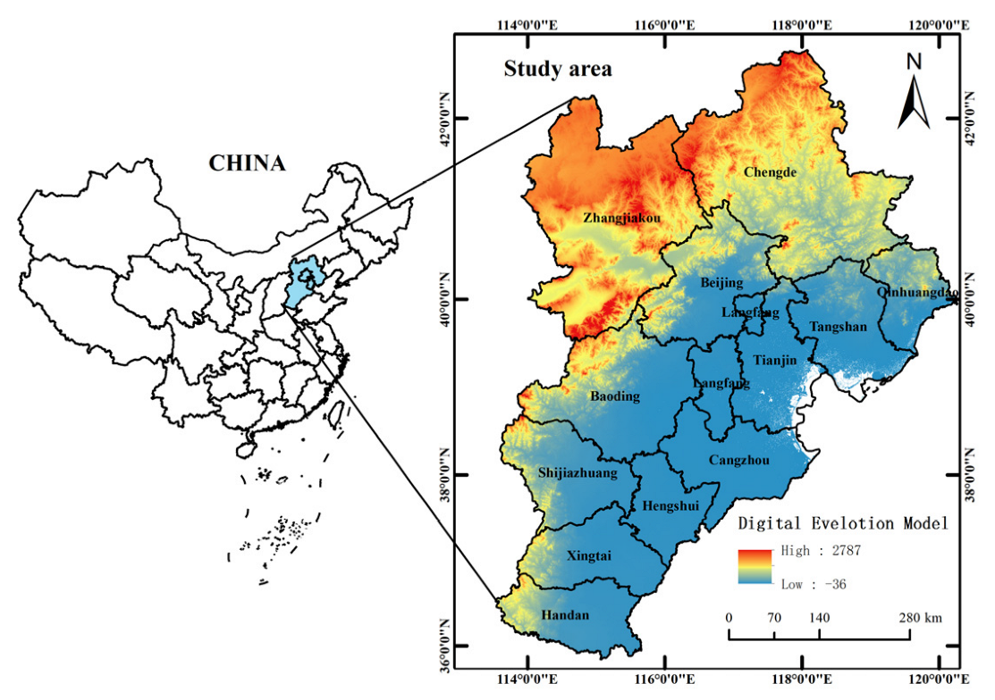
2.1. Study Area

The BTH region is China’s “Capital Economic Circle”, consisting of Beijing, Tianjin, and Hebei Province, with a total area of 218,000 square kilometers (Figure 1). The overall landscape situation is high in the northwest and low in the southeast, dominated by plains, with an average elevation of about 300 m. The dam area and the Yanshan and Taihang Mountains in the west and north are the main ecological barriers of the North China Plain, whose functions of water conservation, soil conservation, and wind and sand control directly affect the security of the ecosystem of the BTH region and even the North China Plain. In 2019, the resident population of the BTH region was 113.08 million, and the regional GDP was CNY 84,580 billion, accounting for 8.54% of the national GDP. Its urbanization rate was 66.7%, with a high urbanization level and population density. Since the proposal of the Coordinated Development Strategy of the BTH region in 2014, the rapid development of the BTH region urban agglomeration has led to more prominent conflicts between humans and land, which objectively requires studying ULUE and analyzing the relationship between it and EDL to provide suggestions for optimizing land resource allocation and achieving sustainable synergistic development in the BTH region.

2.2. Data Sources and Indicator Selection

2.2.1. Data Sources

The basic data in this paper mainly include the following categories: (1) ULUE input and output indicators data were collected from the “China Urban Statistical Yearbook” from 2000 to 2020, in which the missing indicator data of some cities in the yearbook were replaced by the mean method and linear interpolation method for calculation. (2) The vector data of administrative boundaries of municipalities were obtained from the Resource and Environment Science and Data Center. (3) DEM raster data of 30 m × 30 m were obtained from the Geospatial Data Cloud.

2.2.2. Indicator Selection

ULUE, as an indicator to measure the relative amount of input and output in the process of land use [28], is essentially the sum of economic, social, and ecological benefits that can be generated by the input of a unit area of land [34]. Based on this, the evaluation of ULUE should not only focus on desirable outputs, such as economic, social, and ecological benefits of the land use process, but also consider undesirable outputs resulting from the land use process [35]. Combining the previous research results and the development status of the BTH region, this paper selected the construction land area, fixed asset investment, and persons employed in urban non-private units per year to quantify the input indicators of ULUE, GDP, average wage, and area of green land to quantify the desirable output indicators of ULUE. Meanwhile, sulfur dioxide emissions, industrial wastewater emissions, and industrial soot emissions were selected to quantify the undesirable output indicators. Relevant details of indicators are listed in Table 1.

2.3. Methodology

2.3.1. Super Efficiency SBM Model

The super efficiency SBM model has the following advantages over the traditional data envelopment analysis (DEA) model [15,27,28]: (1) Slack variables are added to the SBM model with undesirable outputs, which can effectively solve the measurement error caused by the traditional radially oriented DEA model [36]. (2) When using the traditional DEA model to measure the efficiency, there are multiple decision-making units with an efficiency value of 1, and it is impossible to compare and rank the decision-making units in DEA effectively. The super efficiency SBM model is proposed to solve this problem [37]. Firstly, the decision-making units with an efficiency value of 1 are eliminated, and secondly, the super efficiency value is derived from the frontier surface composed of the remaining decision-making units, at which time the super efficiency value is generally greater than 1 and can be further compared. The super efficiency SBM model can incorporate multiple undesirable output indicators into the ULUE evaluation system and can more accurately evaluate the ULUE where undesirable output problems exist. Its model expression is as follows:
ULUE = m i n ( 1 1 m i = 1 m S i x i k ) 1 + 1 p 1 + p 2 ( r = 1 p 1 S r + y r k + h = 1 p 2 S h b b h k )
s . t . { x k = X λ + S y k = Y λ S + b k = B λ + S b λ 0 ,   S 0 ,   S + 0 ,   S b 0
where each city represents a decision-making unit. Each decision-making unit contains m inputs, p1 desirable outputs, and p2 undesirable outputs; S, S+, and Sb represent the slack variables of inputs, desirable outputs, and undesired outputs, respectively; X, Y, and B represent the input matrix, desirable output matrix, and undesirable output matrix, respectively; λ represents the weight vector; and ULUE is the urban land use efficiency of each city in the study area. The larger the ULUE, the higher the efficiency.

2.3.2. Coefficient of Variation

The coefficient of variation is applied to quantify the degree of variation of ULUE in the BTH region, and the calculation formula is as follows:
CV = i = 1 n ( X i X ) 2 n X
where CV is the coefficient of variation value; Xi is the ULUE value of each city in the BTH region; X is the average value of ULUE of each city during the study period; n is the number of cities. A larger CV value indicates a larger difference in ULUE among cities and a poorer equilibrium; a smaller CV value indicates a smaller difference in ULUE among cities and a better equilibrium. The CV values on the time series can be used to characterize the trend of heterogeneity or convergence in the development of ULUE in the BTH region [38].

2.3.3. Gravity Center Model

The gravity center characterizes the spatially distributed point of synergy of an object element, which can be regarded to some extent as the focal point of a phenomenon or activity in the region [39]. The migration of the gravity center can characterize the spatial evolution of an object element and reflect the trend of the development of a phenomenon or activity in the region [40]. In this paper, we study the gravity center of ULUE in the BTH region based on the gravity center model and explain the development direction of ULUE in the BTH region by quantifying the migration distance of the gravity center. The calculation formula is as follows:
l o n t = i = 1 n u l u e i t l o n i i = 1 n u l u e i t
l a t t = i = 1 n u l u e i t l a t i i = 1 n u l u e i t
d = ρ l o n t + m l o n t 2 + l a t t + m l a t t 2
where (loni, lati) is the longitude and latitude coordinates of the city i, respectively, ulueit is the urban land use efficiency of the city i in year t, (lont, latt) is the longitude and latitude coordinates of the gravity center of ULUE in year t of the BTH region, respectively, and d is the migration distance of the gravity center from year t to year t + m.

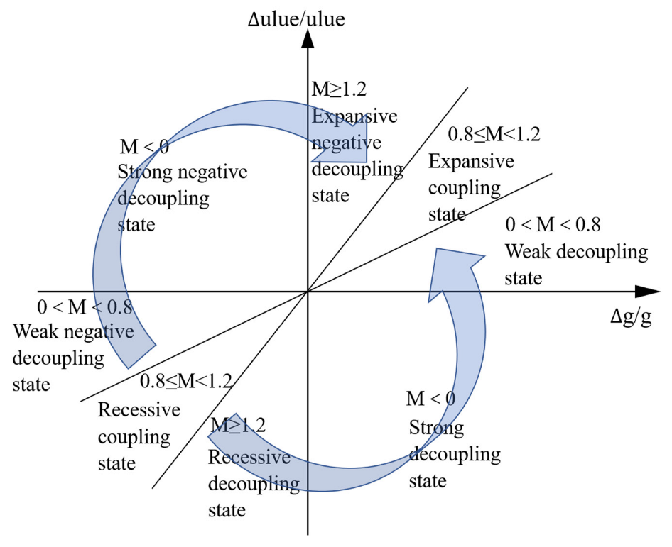
2.3.4. Tapio Decoupling Model

The Tapio decoupling model can be used to analyze the response relationship between the two variables [41]. In this paper, the relationship between ULUE and EDL in the BTH region is studied based on the Tapio decoupling model. The model is constructed as follows:
M t = Δ u l u e / u l u e Δ g / g = ( u l u e t + 1 u l u e t ) / u l u e t ( g t + 1 g t ) / g t
where Mt is the decoupling index between ULUE and EDL; Δulue, Δg are the amount of ULUE change and GDP change from t to t + 1 time period; uluet, gt are the ULUE and GDP at the beginning of the time period, respectively; and uluet+1, gt+1 are the ULUE and GDP at the end of the time period, respectively. Referring to the existing research results, the criteria for defining the decoupling state of the study were determined as shown in Table 2 and Figure 2.

2.3.5. Environmental Kuznets Curve Model

The environmental Kuznets curve (EKC) is a model proposed by the American economists Grossman and Kneger in 1991 to explain economic development and environmental pollution [42]. After the EKC model was proposed, many scholars extended the application of the EKC model to other fields [43,44,45,46,47]. In recent years, some scholars have introduced the EKC model into the field of land use, for example, Qu et al. (2022) analyzed the relationship between intensive rural land use and agricultural nonpoint source pollution based on the Tapio model and the EKC model [48]. Esposito et al. (2018) analyzed the U-shaped EKC relationship between land consumption and economic development based on an econometric model [49]. Therefore, in order to further clarify the relationship between ULUE and EDL in the BTH region, this paper applies panel data to conduct EKC curve research based on the theoretical study of EKC curve and the expansion of related fields [50], and the expression is as follows:
E 1 : u l u e t = λ 0 + λ 1 g t + λ 2 g t 2 + λ 3 g t 3
E 2 : u l u e t = λ 0 + λ 1 g t + λ 2 g t 2
where uluet is the urban land use efficiency (ULUE) at time t, gt is the GDP at time t, and GDP represents the level of urban economic development (EDL). λ0, λ1, λ2, λ3 are constant terms, and different positive and negative combinations of λ1, λ2, λ3 will affect the shape of the final curve.

3. Results

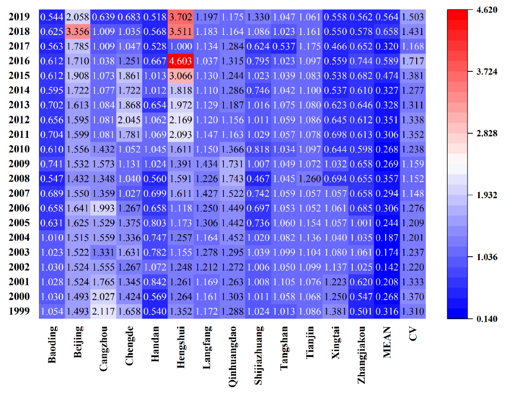
3.1. Analysis of Spatiotemporal Evolution Characteristics of ULUE

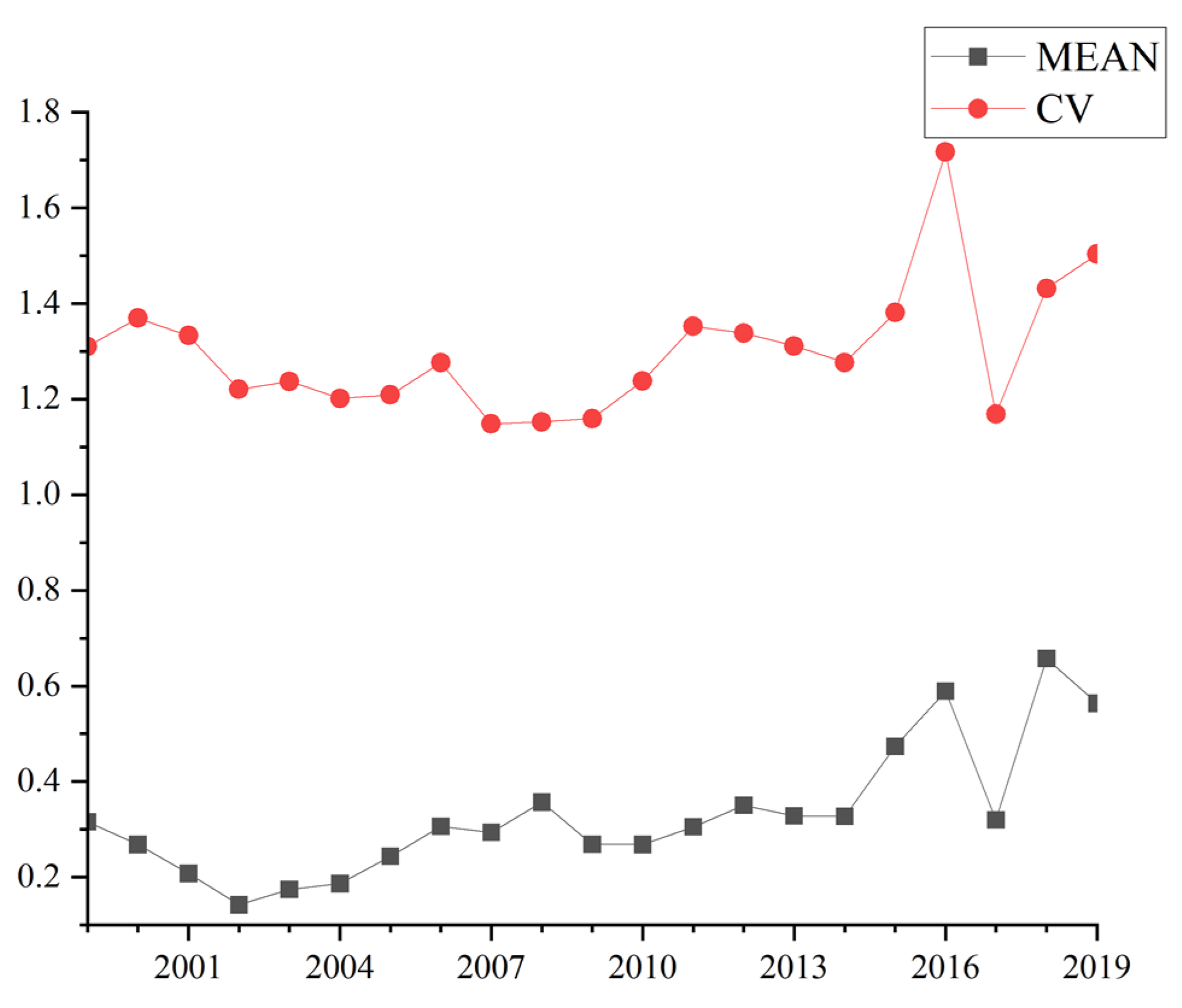
3.1.1. Temporal Evolution Characteristics of ULUE

In this paper, we measured the ULUE of the BTH region from 1999 to 2019 based on MaxDEA software (The publisher is in Beijing, China), and calculated the average value of ULUE and its coefficient of variation by year; the results are shown in Figure 3 and Figure 4.
Firstly, it can be seen from Figure 3 that the decrease rates of ULUE from 1999 to 2019 in Baoding, Cangzhou, Chengde, Handan, Qinhuangdao, Tianjin, and Xingtai were 48.4%, 69.83%, 58.78%, 4.06%, 8.76%, 2.25%, and 59.6%, respectively, while the increase rates of ULUE in Beijing, Hengshui, Langfang, Shijiazhuang, Tangshan, and Zhangjiakou from 1999 to 2019 were 37.82%, 173.72%, 2.1%, 29.83%, 3.35%, and 12.3%, respectively. In other words, Hengshui had the largest increase in ULUE, while Cangzhou had the largest decrease in ULUE, and Hengshui had the highest ULUE in 2016.
As can be seen from Figure 4, the ULUE of the BTH region showed a fluctuating upward trend from 1999 to 2019, and its lowest and highest inflection points appeared in 2002 and 2018, respectively. Before 2002, the mean ULUE of 13 cities decreased year by year, from 0.316 in 1999 to 0.142 in 2002, with an average annual decrease rate of 23.41%. From 2002 to 2016, the average ULUE increased from 0.142 to 0.589, with an average annual growth rate of 10.7%. From 2016 to 2019, the ULUE showed a ‘horizontal S’ trajectory, first dropping sharply in 2017, then rising to the highest value in 20 years in 2018, and then dropping in 2019. Meanwhile, from the coefficient of variation of ULUE in each year, the overall difference of ULUE in the BTH region increased from 1.31 in 1999 to 1.503 in 2019, indicating that the dispersion of ULUE in each city has been increasing and spatial heterogeneity has gradually appeared.

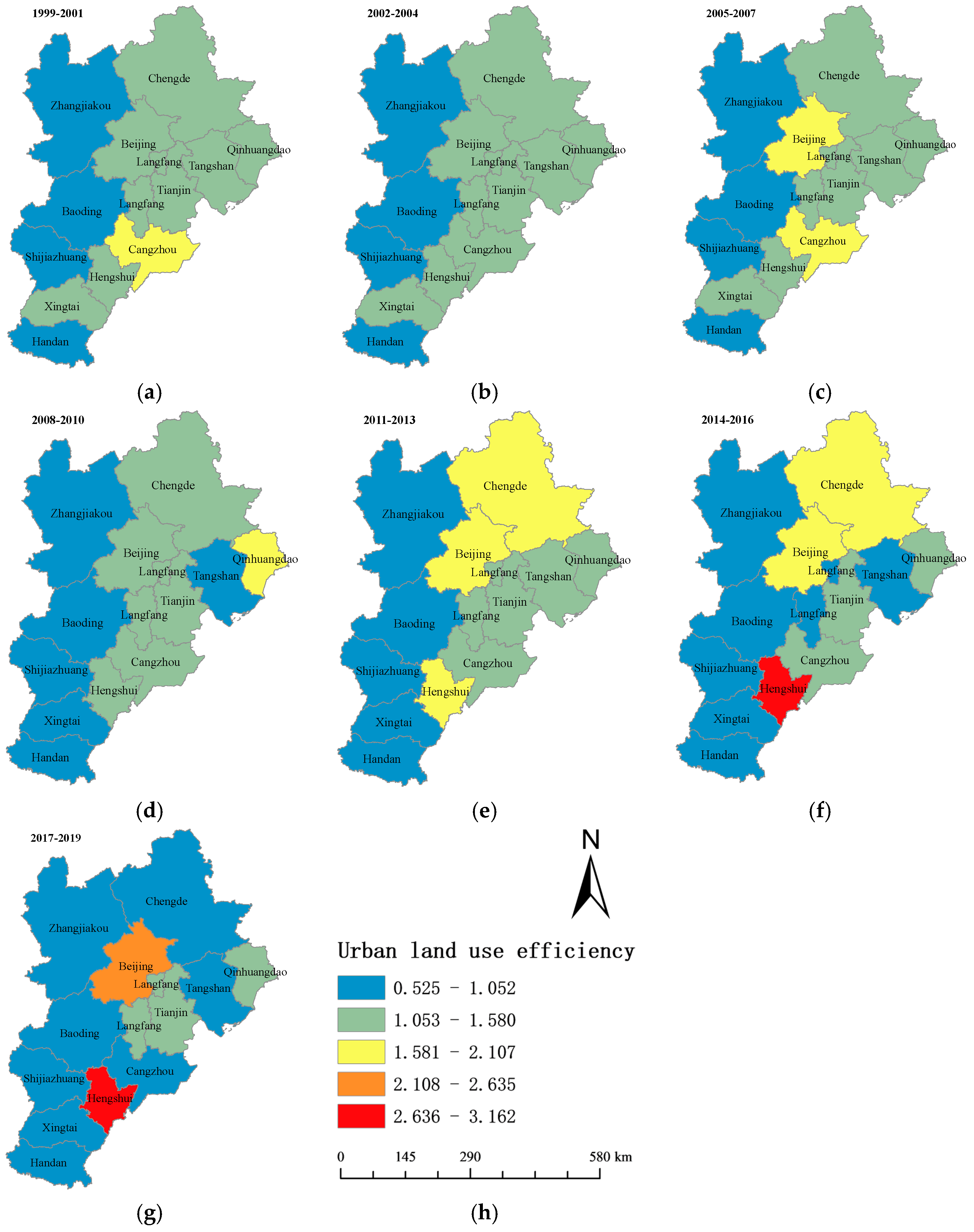
3.1.2. Spatial Distribution Characteristics of ULUE

To further study the spatial characteristics of ULUE, this paper divided the period 1999 to 2019 into seven stages, with one stage spanning three years (Figure 5). From the spatial scale, the ULUE of the BTH region had a distribution pattern of “high in the southeast and low in the northwest”, and the differentiation of ULUE among cities was gradually significant during the study period.
Considering the geographical background of each city, the eastern cities of Qinhuangdao, Tangshan, Tianjin, and Cangzhou are located along the Bohai Sea, the coastal geographical background has promoted local economic development, and the limited land resources have also promoted land intensification in the region to a certain extent, which has improved the ULUE of these cities. Baoding, Shijiazhuang, Xingtai, and Handan, as inland cities in the BTH region, have a weaker frequency of resource exchange and economic industry types than coastal areas. Thus, economic development is slower, and economic backwardness leads to the phenomenon of land finance through income from the concession of land use rights to maintain local fiscal expenditures and the expansion of construction land by attracting projects at lower land prices, resulting in excessive waste of land. Beijing, as the economic, cultural, and political center of China, has a strong contradiction between people and land [51], and the development and utilization of land in three dimensions (i.e., surface, above, and below ground) has greatly improved the efficiency of land resources.
The coordinates of the gravity center, the migration direction, and the migration distance of the ULUE in the BTH region were obtained according to the calculation method of the gravity center model, and these are shown in Table 3. In 1999 to 2019, the gravity center of the ULUE in the BTH region was located near the geometric center of the BTH region (116°18′40″ E, 39°04′10″ N), showing spatial equilibrium. From the migration direction and migration distance of the gravity center of ULUE from 1999 to 2019, the ULUE had migrated in northwest, southeast, and southwest directions, but the migration differences in the northwest direction were larger than those in the southeast and southwest directions, indicating that the differences in ULUE were mainly reflected in the northwest cities. However, these differences were not sufficient to induce the gravity center of ULUE to undergo longer distance migration. At the same time, the gravity center of ULUE shifted the largest distance in the southeast direction from 2004 to 2007, indicating that the ULUE differences in the southeast increased in that period.

3.2. Relationship between ULUE and EDL

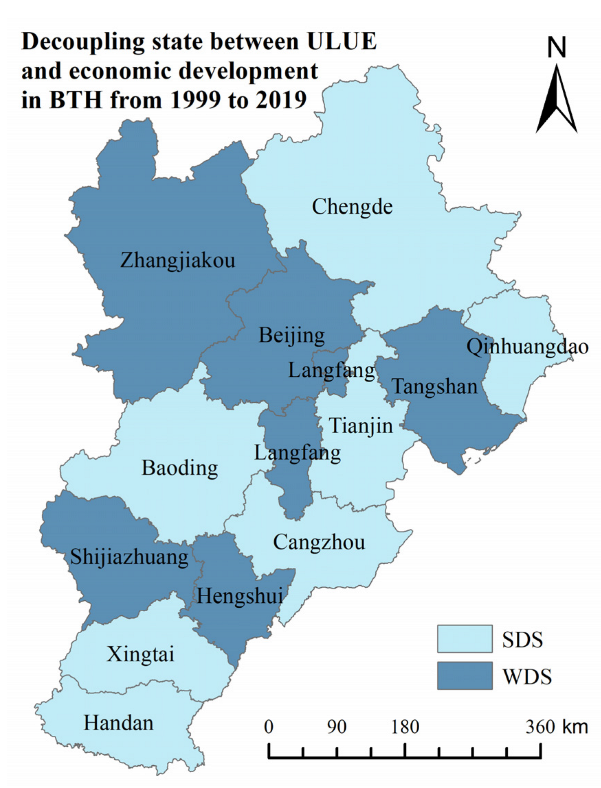
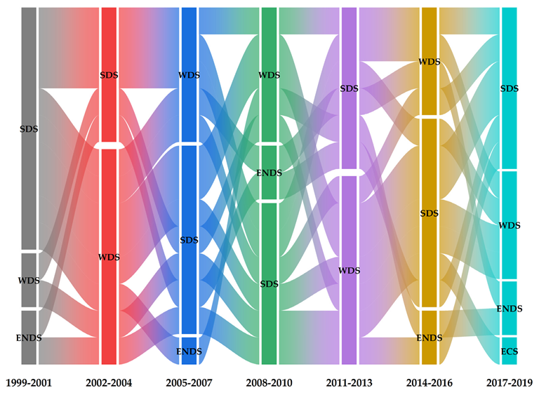
3.2.1. Decoupling Analysis of the ULUE and EDL

The Tapio model was used to explore the relationship between ULUE and EDL in the BTH region, and the decoupling index was first calculated with a window width of 3 years (except the first and last years). Then, the decoupling index was calculated for the whole study period, and the decoupling states were classified according to Table 2. The results of the decoupling states calculated with a window width of 3 years are shown in Figure 6.
From 1999 to 2019, the relationship between ULUE and EDL in the BTH region mainly showed four states, namely, strong decoupling state (SDS), weak decoupling state (WDS), expansive negative decoupling state (ENDS), and expansive coupling state (ECS). From the horizontal evolution structure of the decoupling relationship in Figure 6, the relationship between ULUE and EDL in the BTH region fluctuated repeatedly between decoupling state and coupling state. As of 2019, there were still a small number of cities in SDS, but overall, it basically showed a transitioning trend from decoupling state to coupling state in the end, that is, during 20 years, with the development of economy, ULUE was on the rise, which is consistent with the description in Section 3.1.1. The increase in ULUE may depend on the implementation of relevant land management measures by the government, but a series of scientific and technological measures and policy instruments are still needed to improve ULUE in the future, in order to maintain the stability of the coupling relationship and promote the coordinated development of ULUE and the economy. From the perspective of the vertical composition structure of the decoupling relationship shown in Figure 6, there was spatial heterogeneity in the decoupling relationship among different cities in each time period.
The spatial distribution of the decoupling relationship between ULUE and EDL was quantified for 13 cities in the BTH region with a window width of the whole study period, as shown in Figure 7. Over 20 years, the seven cities, Chengde, Qinhuangdao, Tianjin, Baoding, Cangzhou, Xingtai, and Handan, showed SDS and a negative correlation between ULUE and EDL, and therefore need to formulate relevant policies to improve ULUE. The six cities, Zhangjiakou, Beijing, Langfang, Tangshan, Shijiazhuang, and Hengshui showed WDS, and their ULUE was in an upward trend, but the rising rate is far lower than the rate of EDL, that is, the economic development trend is good, but there is still a great potential to improve the land use efficiency.

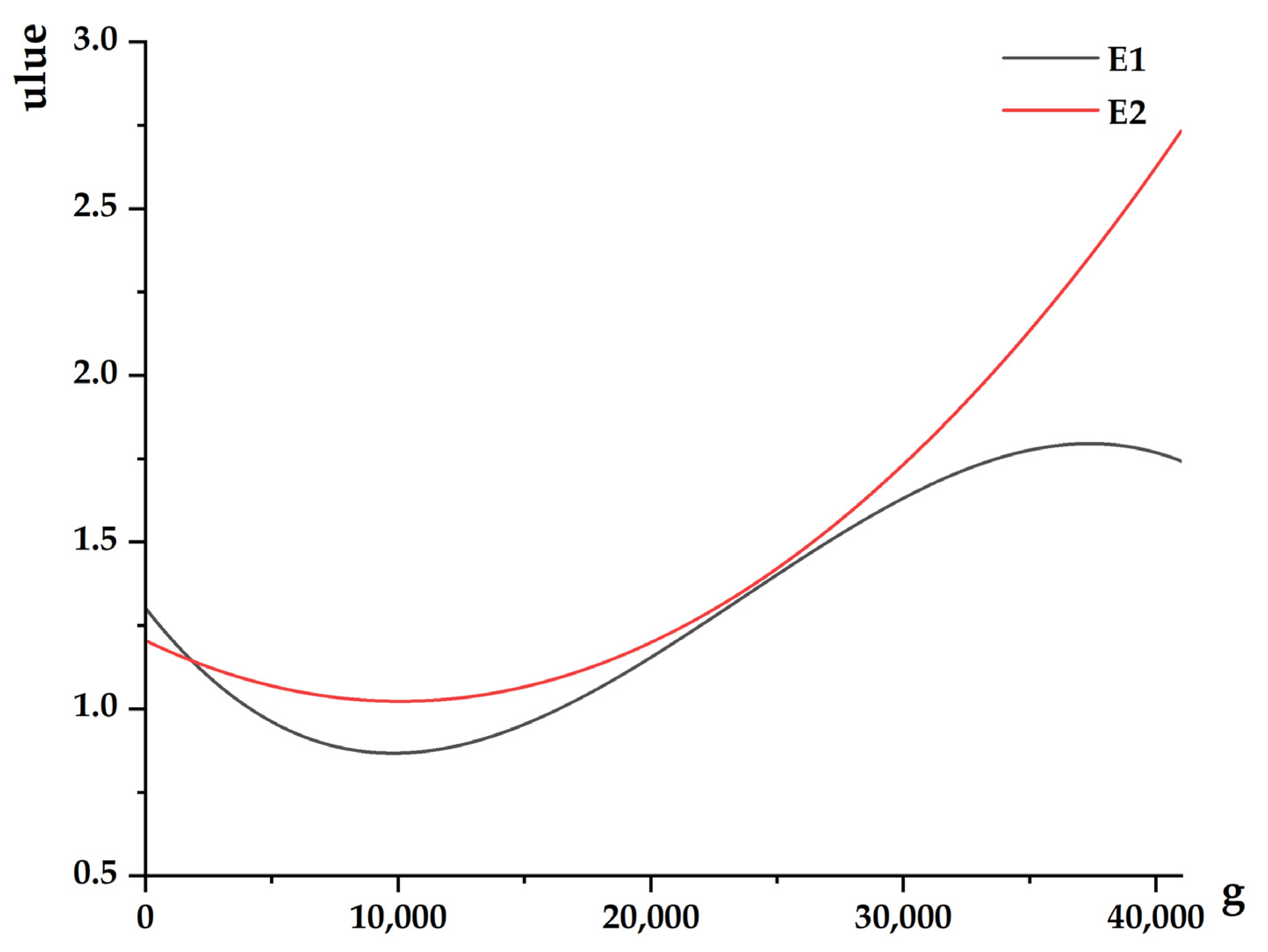
3.2.2. EKC Curve Relationship Test between ULUE and EDL

Before establishing the EKC model, the panel data of ULUE and EDL need to be subjected to a unit heel test to assess the data’s smoothness. In this paper, an ADF test, PP test, and IPS test were conducted on the panel data based on EViews 8 software (The publisher is in Englewood, USA), and the tests showed that the first-order difference values of all variables were significant at the 1% test level. A Pedroni cointegration test was conducted on this basis, and the results showed that all variables had cointegration relationships. By Hausman test, the original hypothesis of random effect was rejected, and a fixed effect regression model was adopted. The model estimation results are shown in Table 4. The E1 and E2 regression models are as follows. Since the correlation coefficient of the three-term g3 of the E1 model is not significant, the E2 model was used for analysis in this paper.
E 1 : u l u e t = 1.302924 ( 9.74   ×   10 5 ) g t + ( 6.27   ×   10 9 ) g t 2 ( 8.86   ×   10 14 ) g t 3
E 2 : u l u e t = 1.204806 ( 3.61   ×   10 5 ) g t + ( 1.79   ×   10 9 ) g t 2
From the E2 curve in Figure 8, it can be seen that between 1999 and 2019, ULUE and EDL showed a EKC “U-shaped” curve, and its inflection point was (10,083.81, 1.02). Moreover, the inflection point of the E1 curve was also located near the EDL value of 10,000. This indicates that the ULUE decreases with the increases in EDL before the inflection point of EDL, which may be due to the excessive land use by the local government in the early stage of economic development due to the excessive pursuit of economic growth and the granting of a large amount of land to attract investment [52,53]. After the EDL value reaches the inflection point, the ULUE increases with the increases in EDL, which may be due to the limited urban land resources at a certain stage of economic development and related policies that gradually intensify land use and thus improve ULUE [54]. The EKC “U” curve reflects the development process of “increasing the quantity of land use first, and then improving the quality of land use”, and also implies the transformation of the relationship between ULUE and EDL from “decoupling state” to “coupling state”, which is also consistent with the analysis of the decoupling results in Section 3.2.1. The EKC curve model is arguably a complementary illustration of the above decoupling analysis.

4. Discussion

4.1. ULUE in the BTH Region

From 1999 to 2019, the ULUE of the BTH region as a whole showed a fluctuating upward trend, with its lowest and highest inflection points occurring in 2002 and 2018, respectively, in which land policy played an important role [55].
On the one hand, some scholars have shown that the marketization of land transfer can improve the ULUE [56], which can explain the fluctuating upward trend of ULUE in this paper (Figure 4). In 1999, China issued a series of relevant policies, such as the “Notice on Further Implementation of Bidding and Auction for the Transfer of State-owned Land Use Right”, “Several Opinions on Standardizing State-owned Land Leasing”, and “Provisional Regulations on the Transfer and Transfer of State-owned Land Use Right in Towns”, all of which were intended to improve the method of using land use rights for compensation, but in reality, administrative allocation and agreement granting were still the most important methods of land supply at that time, and the market mechanism could hardly be mobilized, which might also be a reason for the low ULUE. At the end of 2001, China joined the WTO and began to promote the marketization of the economy as a whole, and land, as an important factor of production, also participated in the reform of the market. Moreover, the former Ministry of Land and Resources issued the “Catalogue of Allocated Land”, specifying that construction land not conforming to the allocated catalogue should be used for compensation, seeking to change the situation of low market allocation of land assets. Due to the time lag of the policy [57], the ULUE was still not high at the end of 2002, but after 2002, the ULUE began to gradually improve, the market mechanism gradually started to operate, and operational construction land gradually transitioned from non-market to market allocation. After that, China gradually improved the secondary market of land transfer, mortgage, and lease, and issued policy documents such as the “Notice on Promoting Economical and Intensive Land Use” and “Guiding Opinions on Promoting Economical and Intensive Land Use”, which to a certain extent promoted the enhancement of ULUE afterwards.
On the other hand, some scholars have suggested that urban agglomeration development could exert a beneficial “1 + 1” >2 effect on cities and contribute to the improvement of economic performance among cities within urban agglomerations [58]. Meanwhile, some scholars believe that urban agglomerations can achieve economic growth without expanding urban land area, thereby improving ULUE [59,60,61,62], which was why ULUE increased after the BTH region Coordinated Development Strategy was proposed by China in 2014. However, other scholars argue that the development of urban agglomerations then represents a larger-scale reuse and remodeling of land resources, which may have a series of negative ecological effects [63,64]. We can combine these two different views, carry out deeper research on policies related to the coordinated development of the BTH urban agglomeration, strengthen scientific and technological innovation, and achieve urban economic growth while reducing the negative effects of land remodeling, thus improving ULUE and ensuring the synergistic development of ULUE and economy.
In terms of spatial distribution, ULUE had a distribution pattern of “high in the southeast and low in the northwest”, and the relevant literature shows that the geographical characteristics of cities in terms of natural resource endowment and socioeconomic structure are very important for ULUE [65], which supports the research results of spatial distribution pattern of ULUE in the BTH region in this paper.

4.2. Spatial Distribution Characteristics of Decoupling Relationship

It can be seen from Figure 7 that from 1999 to 2019, the decoupling relationship between ULUE and EDL in the BTH region was closely related to its spatial location. From the north to the south, it was SDS, WDS, SDS, and WDS, showing a regular interval repetition distribution pattern. At the same time, the cities showing SDS and the cities showing WDS showed agglomeration effects in spatial distribution. Referring to the first law of geography [66], the main reason may be that these cities are closer in spatial location, and their ULUE as well as EDL may be more similar, so these cities presented a consistent decoupling state. Moreover, some related research found that there is a significant spatial spillover effect of ULUE [16]. As can be seen from Figure 6, the decoupling relationship between ULUE and EDL improved in 2014, after the BTH region Coordinated Development Strategy was proposed, which indicates that the agglomeration development of urban clusters can promote the synergistic development of ULUE and EDL to a certain extent and improve their decoupling state.

4.3. EKC “U-Shaped” Curve Model

The curve relationship test between ULUE and EDL can be fitted and simulated by the EKC model. This model is consistent with the “U-shaped” curve model (E2 curve in Figure 8), and also conforms to the change rule of the “N-shaped” curve model (E1 curve in Figure 8). This is because, over a long time scale, the “U-shaped” curve may only be a part of the “N-shaped” curve or the “M-shaped” curve (i.e., the possibility of multiple inflection points). After crossing the first inflection point, EDL will still lead to a decrease in ULUE. However, in this paper, from the specific time period 1999 to 2019, the values of EDL in the BTH region are taken to range from 159 to 35,371, and both E1 and E2 curves show a “U-shaped” curve relationship between ULUE and EDL. That is, as the EDL increases, the ULUE tends to decrease first and then increase. This is also consistent with Xue et al. (2022), who showed a “U-shaped” curve relationship between economic development and ULUE in the Yellow River basin [15]. However, the relationship between ULUE and EDL is spatially heterogeneous [30], and the relationship between them may be an inverted “U-shape” in other regions, for example, Han et al. (2020) found an inverted “U-shaped” relationship between economic development and ULUE at the national scale [30]. That is, as the economy grows, the efficiency of ULUE may first increase rapidly, then grow slowly, and then level off or even decline.

4.4. Research Limitations and Prospects

The influence factors and driving mechanisms of ULUE are complex, and the selected indicators are important for quantifying the results. This paper quantified the ULUE of the BTH region based on the super efficiency SBM model with reference to the selection of indicators from other related research, but no sensitivity or robustness analysis was conducted on the ULUE results based on the software MaxDEA. At the same time, with regard to the scale of the study (such as provincial, municipal, county, township, and even grid scale), whether the measurement of ULUE will be different at different scales in the same region, which scale is the most accurate at quantifying ULUE, and which scale we should use to quantify ULUE are all worthy of further consideration and research.

5. Conclusions

In this study, we quantified the ULUE of the BTH region from 1999 to 2019 based on the super efficiency SBM model, considering the undesirable output of land use, and analyzed the decoupling state of ULUE and EDL over 20 years by combining the Tapio decoupling model, and analyzed the nonlinear relationship between ULUE and EDL by constructing the EKC model. The main research results are summarized as follows.
In 1999–2019, from the temporal scale, the ULUE of the BTH region shows a fluctuating upward trend, with the lowest and highest inflection points appearing in 2002 and 2018, respectively, and the differentiation of ULUE among cities is gradually significant. From the spatial scale, the ULUE of BTH region has a spatial distribution pattern of “high in the southeast and low in the northwest”, and the eastern coastal cities of Qinhuangdao, Tangshan, Tianjin, and Cangzhou have relatively faster economic development and higher ULUE. The cities of Baoding, Xingtai, Shijiazhuang, and Handan in the west have weaker resource exchange frequency and economic industry type than the coastal areas, so their economic development is slower and their ULUE is lower.
In 1999–2019, from the temporal scale, the decoupling relationship between ULUE and EDL in the BTH region shows repeated fluctuations between the decoupling state and coupling state, but overall, it basically shows a transition trend from decoupling state to coupling state in the end. From the spatial scale, the decoupling relationships are SDS, WDS, SDS, and WDS from north to south, showing a regular interval repetitive distribution pattern, while cities presenting as SDS and cities presenting as WDS show clustering distribution in space. Seven cities, namely, Chengde, Qinhuangdao, Tianjin, Baoding, Cangzhou, Xingtai, and Handan, exhibit SDS, which shows a negative correlation between ULUE and economic growth, and therefore need to formulate relevant policies to improve ULUE. Six cities, namely, Zhangjiakou, Beijing, Langfang, Tangshan, Shijiazhuang, and Hengshui, exhibit WDS, and their ULUE has an increasing trend, but the rate of increase is much lower than the rate of increase of EDL.
The relationship between ULUE and EDL in the BTH region presents a “U-shaped” EKC curve, that is, ULUE decreases first and then increases with the increases of EDL. EKC “U-shape” reflects the economic development process of “increasing the quantity of land use first, and then improving the quality of land use”.
Based on the above research findings, the following insights can be obtained: (1) Local governments should combine relevant national land policies, optimize urban land resource allocation, strengthen law enforcement and disposal of low-utility land, and improve the secondary land market to revitalize stock land resources and promote effective land transfer. (2) Strengthen scientific technological innovation, explore the development and utilization of non-traditional agricultural land resources, efficient and intensive urban construction land utilization (such as the utilization of urban three-dimensional space), reuse technology of abandoned land resources, etc., and thus improve the efficiency of land resource utilization. (3) Strengthen the linkage development between the BTH urban agglomerations, promote the flow of resource elements between cities in the east and west as well as between industries, so that the economic ties between cities can be gradually strengthened, drive the full utilization of limited land resources through the economy, and thus improve the efficiency of land resources while developing the economy.

Author Contributions

Conceptualization, S.L., Y.X. and C.W.; methodology, S.L., Y.X., C.W., M.F. and Y.T.; software, S.L., Y.X. and C.W.; formal analysis, S.L., Y.X. and C.W.; investigation, S.L, Y.X. and C.W.; data curation, S.L., Y.X. and C.W.; writing—original draft preparation, S.L., Y.X., C.W., M.F. and Y.T.; writing—review and editing, S.L. and M.F.; visualization, S.L.; project administration, M.F. All authors have read and agreed to the published version of the manuscript.

Funding

This research received no external funding.

Institutional Review Board Statement

Not applicable.

Informed Consent Statement

Not applicable.

Data Availability Statement

Not applicable.

Acknowledgments

Thanks for the constructive suggestions from editor and anonymous reviewers, which were helpful for improving our research.

Conflicts of Interest

The authors declare no conflict of interest.

References

  1. Li, Y.; Li, Y.; Westlund, H.; Liu, Y. Urban-rural transformation in relation to cultivated land conversion in China: Implications for optimizing land use and balanced regional development. Land Use Policy 2015, 47, 218–224. [Google Scholar] [CrossRef]
  2. Cheng, L.; Jiang, P.; Chen, W.; Li, M.; Wang, L.; Gong, Y.; Pian, Y.; Xia, N.; Duan, Y.; Huang, Q. Farmland protection policies and rapid urbanization in China: A case study for Changzhou City. Land Use Policy 2015, 48, 552–566. [Google Scholar] [CrossRef]
  3. Urban Growth Models: Progress and Perspective|SpringerLink. Available online: https://link.springer.com/article/10.1007/s11434-016-1111-1 (accessed on 6 May 2022).
  4. Yin, C.; Meng, F.; Yang, X.; Yang, F.; Fu, P.; Yao, G.; Chen, R. Spatio-temporal evolution of urban built-up areas and analysis of driving factors—A comparison of typical cities in north and south China. Land Use Policy 2022, 117, 106114. [Google Scholar] [CrossRef]
  5. Chen, H.; Tan, Y.; Xiao, W.; Li, G.; Meng, F.; He, T.; Li, X. Urbanization in China drives farmland uphill under the constraint of the requisition–compensation balance. Sci. Total Environ. 2022, 831, 154895. [Google Scholar] [CrossRef] [PubMed]
  6. Meng, F.; Wang, D.; Meng, X.; Li, H.; Liu, G.; Yuan, Q.; Hu, Y.; Zhang, Y. Mapping urban energy–water–land nexus within a multiscale economy: A case study of four megacities in China. Energy 2022, 239, 122038. [Google Scholar] [CrossRef]
  7. Zhang, Y.; Liu, Y.; Zhang, Y.; Kong, X.; Jing, Y.; Cai, E.; Zhang, L.; Liu, Y.; Wang, Z.; Liu, Y. Spatial Patterns and Driving Forces of Conflicts among the Three Land Management Red Lines in China: A Case Study of the Wuhan Urban Development Area. Sustainability 2019, 11, 2025. [Google Scholar] [CrossRef] [Green Version]
  8. Liu, T.; Liu, H.; Qi, Y. Construction land expansion and cultivated land protection in urbanizing China: Insights from national land surveys, 1996–2006. Habitat Int. 2015, 46, 13–22. [Google Scholar] [CrossRef]
  9. Babenko, V.; Zomchak, L.; Nehrey, M. Ecological and economic aspects of sustainable development of Ukrainian regions. E3S Web Conf. 2021, 280, 02003. [Google Scholar] [CrossRef]
  10. Farafonova, N.V. Essence and Components of Economic Efficiency of Business Activities Within Agrarian Sector. Actual Probl. Econ. 2011, 124, 176–185. [Google Scholar]
  11. Ren, C. Discussion on the Relationship of Administrative Efficiency and Administrative Efficacy. In Proceedings of the 2014 International Conference on Global Economy, Finance and Humanities Research, Tianjin, China, 27–28 March 2014; Zheng, F., Ed.; Atlantis Press: Paris, France, 2014; Volume 112, pp. 238–240. [Google Scholar]
  12. Liu, J.; Jin, X.; Xu, W.; Gu, Z.; Yang, X.; Ren, J.; Fan, Y.; Zhou, Y. A new framework of land use efficiency for the coordination among food, economy and ecology in regional development. Sci. Total Environ. 2020, 710, 135670. [Google Scholar] [CrossRef]
  13. Herzig, A.; Nguyen, T.T.; Ausseil, A.-G.E.; Maharjan, G.R.; Dymond, J.R.; Arnhold, S.; Koellner, T.; Rutledge, D.; Tenhunen, J. Assessing resource-use efficiency of land use. Environ. Model. Softw. 2018, 107, 34–49. [Google Scholar] [CrossRef]
  14. Li, Q.; Wang, Y.; Chen, W.; Li, M.; Fang, X. Does improvement of industrial land use efficiency reduce PM2.5 pollution? Evidence from a spatiotemporal analysis of China. Ecol. Indic. 2021, 132, 108333. [Google Scholar] [CrossRef]
  15. Xue, D.; Yue, L.; Ahmad, F.; Draz, M.U.; Chandio, A.A.; Ahmad, M.; Amin, W. Empirical investigation of urban land use efficiency and influencing factors of the Yellow River basin Chinese cities. Land Use Policy 2022, 117, 106117. [Google Scholar] [CrossRef]
  16. Zhang, W.; Wang, B.; Wang, J.; Wu, Q.; Wei, Y.D. How does industrial agglomeration affect urban land use efficiency? A spatial analysis of Chinese cities. Land Use Policy 2022, 119, 106178. [Google Scholar] [CrossRef]
  17. Jingxin, G.; Jinbo, S.; Lufang, W. A new methodology to measure the urban construction land-use efficiency based on the two-stage DEA model. Land Use Policy 2022, 112, 105799. [Google Scholar] [CrossRef]
  18. Meng, Y.; Zhang, F.-R.; An, P.-L.; Dong, M.-L.; Wang, Z.-Y.; Zhao, T. Industrial land-use efficiency and planning in Shunyi, Beijing. Landsc. Urban Plan. 2008, 85, 40–48. [Google Scholar] [CrossRef]
  19. Baráth, L.; Fertő, I. Heterogeneous technology, scale of land use and technical efficiency: The case of Hungarian crop farms. Land Use Policy 2015, 42, 141–150. [Google Scholar] [CrossRef] [Green Version]
  20. Den, X.; Gibson, J. Sustainable land use management for improving land eco-efficiency: A case study of Hebei, China. Ann. Oper. Res. 2020, 290, 265–277. [Google Scholar] [CrossRef]
  21. Built-up land efficiency in urban China: Insights from the General Land Use Plan (2006–2020). Habitat Int. 2016, 51, 31–38. [CrossRef]
  22. Chen, Y. Measuring super-efficiency in DEA in the presence of infeasibility. Eur. J. Oper. Res. 2005, 161, 545–551. [Google Scholar] [CrossRef]
  23. Li, S.; Jahanshahloo, G.R.; Khodabakhshi, M. A super-efficiency model for ranking efficient units in data envelopment analysis. Appl. Math. Comput. 2007, 184, 638–648. [Google Scholar] [CrossRef]
  24. Kuang, B.; Lu, X.; Zhou, M.; Chen, D. Provincial cultivated land use efficiency in China: Empirical analysis based on the SBM-DEA model with carbon emissions considered. Technol. Forecast. Soc. Chang. 2020, 151, 119874. [Google Scholar] [CrossRef]
  25. Jiang, H. Spatial–temporal differences of industrial land use efficiency and its influencing factors for China’s central region: Analyzed by SBM model. Environ. Technol. Innov. 2021, 22, 101489. [Google Scholar] [CrossRef]
  26. Lu, X.; Chen, D.; Wang, Y. Is Urban Sprawl Decoupled from the Quality of Economic Growth? Evidence from Chinese Cities. Sustainability 2020, 12, 218. [Google Scholar] [CrossRef] [Green Version]
  27. Saikku, L.; Mattila, T.J. Drivers of land use efficiency and trade embodied biomass use of Finland 2000–2010. Ecol. Indic. 2017, 77, 348–356. [Google Scholar] [CrossRef]
  28. Yu, J.; Zhou, K.; Yang, S. Land use efficiency and influencing factors of urban agglomerations in China. Land Use Policy 2019, 88, 104143. [Google Scholar] [CrossRef]
  29. Cao, X.; Liu, Y.; Li, T.; Liao, W. Analysis of Spatial Pattern Evolution and Influencing Factors of Regional Land Use Efficiency in China Based on ESDA-GWR. Sci. Rep. 2019, 9, 520. [Google Scholar] [CrossRef]
  30. Han, X.; Zhang, A.; Cai, Y. Spatio-Econometric Analysis of Urban Land Use Efficiency in China from the Perspective of Natural Resources Input and Undesirable Outputs: A Case Study of 287 Cities in China. Int. J. Environ. Res. Public Health 2020, 17, 7297. [Google Scholar] [CrossRef] [PubMed]
  31. Wang, X.; Li, R. Is Urban Economic Output Decoupling from Water Use in Developing Countries?-Empirical Analysis of Beijing and Shanghai, China. Water 2019, 11, 1335. [Google Scholar] [CrossRef] [Green Version]
  32. Song, Y.; Sun, J.; Zhang, M.; Su, B. Using the Tapio-Z decoupling model to evaluate the decoupling status of China’s CO2 emissions at provincial level and its dynamic trend. Struct. Chang. Econ. Dyn. 2020, 52, 120–129. [Google Scholar] [CrossRef]
  33. Zhang, M.; Li, H.; Su, B.; Yang, X. Using a new two-dimensional decoupling model to evaluate the decoupling state of global energy footprint. Sustain. Cities Soc. 2020, 63, 102461. [Google Scholar] [CrossRef]
  34. Liu, Y.; Zhang, Z.; Zhou, Y. Efficiency of construction land allocation in China: An econometric analysis of panel data. Land Use Policy 2018, 74, 261–272. [Google Scholar] [CrossRef]
  35. Yang, B.; Wang, Z.; Zou, L.; Zou, L.; Zhang, H. Exploring the eco-efficiency of cultivated land utilization and its influencing factors in China’s Yangtze River Economic Belt, 2001–2018. J. Environ. Manag. 2021, 294, 112939. [Google Scholar] [CrossRef] [PubMed]
  36. Fang, H.-H.; Lee, H.-S.; Hwang, S.-N.; Chung, C.-C. A slacks-based measure of super-efficiency in data envelopment analysis: An alternative approach. Omega-Int. J. Manag. Sci. 2013, 41, 731–734. [Google Scholar] [CrossRef]
  37. Tone, K.; Toloo, M.; Izadikhah, M. A modified slacks-based measure of efficiency in data envelopment analysis. Eur. J. Oper. Res. 2020, 287, 560–571. [Google Scholar] [CrossRef]
  38. Shao, J.; Ge, J. Investigation into Relationship between Intensive Land Use and Urban Heat Island Effect in Shijiazhuang City Based on the Tapio Decoupling Theory. J. Urban Plann. Dev. 2020, 146, 04020043. [Google Scholar] [CrossRef]
  39. Yang, W.; Yaning, C.; Zhi, L. Evolvement Characteristics of Population and Economic Gravity Centers in Tarim River Basin, Uygur Autonomous Region of Xinjiang, China. Chin. Geogr. Sci. 2013, 23, 765–772. [Google Scholar] [CrossRef] [Green Version]
  40. How do population and land urbanization affect CO2 emissions under gravity center change? A spatial econometric analysis. J. Clean. Prod. 2018, 202, 510–523. [CrossRef]
  41. Yasmeen, H.; Tan, Q. Assessing Pakistan’s energy use, environmental degradation, and economic progress based on Tapio decoupling model. Environ. Sci. Pollut Res. 2021, 28, 68364–68378. [Google Scholar] [CrossRef] [PubMed]
  42. Grossman, G.; Krueger, A. Economic-Growth and the Environment. Q. J. Econ. 1995, 110, 353–377. [Google Scholar] [CrossRef] [Green Version]
  43. Xie, Q.; Xu, X.; Liu, X. Is there an EKC between economic growth and smog pollution in China? New evidence from semiparametric spatial autoregressive models. J. Clean. Prod. 2019, 220, 873–883. [Google Scholar] [CrossRef]
  44. Ajanaku, B.A.; Collins, A.R. Economic growth and deforestation in African countries: Is the environmental Kuznets curve hypothesis applicable? For. Policy Econ. 2021, 129, 102488. [Google Scholar] [CrossRef]
  45. Mills Busa, J.H. Dynamite in the EKC tunnel? Inconsistencies in resource stock analysis under the environmental Kuznets curve hypothesis. Ecol. Econ. 2013, 94, 116–126. [Google Scholar] [CrossRef]
  46. Badeeb, R.A.; Lean, H.H.; Shahbaz, M. Are too many natural resources to blame for the shape of the Environmental Kuznets Curve in resource-based economies? Resour. Policy 2020, 68, 101694. [Google Scholar] [CrossRef]
  47. Sesma-Martín, D.; Puente-Ajovín, M. The Environmental Kuznets Curve at the thermoelectricity-water nexus: Empirical evidence from Spain. Water Resour. Econ. 2022, 39, 100202. [Google Scholar] [CrossRef]
  48. Qu, Y.; Zhang, Q.; Zhan, L.; Jiang, G.; Si, H. Understanding the nonpoint source pollution loads’ spatiotemporal dynamic response to intensive land use in rural China. J. Environ. Manag. 2022, 315, 115066. [Google Scholar] [CrossRef]
  49. Esposito, P.; Patriarca, F.; Salvati, L. Tertiarization and land use change: The case of Italy. Econ. Model. 2018, 71, 80–86. [Google Scholar] [CrossRef]
  50. Wang, K.; Zhu, Y.; Zhang, J. Decoupling economic development from municipal solid waste generation in China’s cities: Assessment and prediction based on Tapio method and EKC models. Waste Manag. 2021, 133, 37–48. [Google Scholar] [CrossRef]
  51. Li, Y.; Kong, X.; Zhu, Z. Multiscale analysis of the correlation patterns between the urban population and construction land in China. Sustain. Cities Soc. 2020, 61, 102326. [Google Scholar] [CrossRef]
  52. Hou, S.; Song, L.; Wang, J.; Ali, S. How Land Finance Affects Green Economic Growth in Chinese Cities. Land 2021, 10, 819. [Google Scholar] [CrossRef]
  53. Gao, H. Public land leasing, public productive spending and economic growth in Chinese cities. Land Use Policy 2019, 88, 104076. [Google Scholar] [CrossRef]
  54. Jin, W.; Zhou, C.; Luo, L. Impact of Land Input on Economic Growth at Different Stages of Development in Chinese Cities and Regions. Sustainability 2018, 10, 2847. [Google Scholar] [CrossRef] [Green Version]
  55. Feng, D.; Li, J.; Li, X.; Zhang, Z. The Effects of Urban Sprawl and Industrial Agglomeration on Environmental Efficiency: Evidence from the Beijing-Tianjin-Hebei Urban Agglomeration. Sustainability 2019, 11, 3042. [Google Scholar] [CrossRef] [Green Version]
  56. Chen, W.; Shen, Y.; Wang, Y.; Wu, Q. The effect of industrial relocation on industrial land use efficiency in China: A spatial econometrics approach. J. Clean. Prod. 2018, 205, 525–535. [Google Scholar] [CrossRef]
  57. Bao, H.X.H.; Robinson, G.M. Behavioural land use policy studies: Past, present, and future. Land Use Policy 2022, 115, 106013. [Google Scholar] [CrossRef]
  58. Shen, L.; Cheng, G.; Du, X.; Meng, C.; Ren, Y.; Wang, J. Can urban agglomeration bring “1 + 1 > 2Effect”? A perspective of land resource carrying capacity. Land Use Policy 2022, 117, 106094. [Google Scholar] [CrossRef]
  59. Sun, Y.; Ma, A.; Su, H.; Su, S.; Chen, F.; Wang, W.; Weng, M. Does the establishment of development zones really improve industrial land use efficiency? Implications for China’s high-quality development policy. Land Use Policy 2020, 90, 104265. [Google Scholar] [CrossRef]
  60. Liu, D.; Zheng, X.; Wang, H.; Zhang, C.; Li, J.; Lv, Y. Interoperable scenario simulation of land-use policy for Beijing–Tianjin–Hebei region, China. Land Use Policy 2018, 75, 155–165. [Google Scholar] [CrossRef]
  61. Wong, Z.; Li, R.; Zhang, Y.; Kong, Q.; Cai, M. Financial services, spatial agglomeration, and the quality of urban economic growth-based on an empirical analysis of 268 cities in China. Financ. Res. Lett. 2021, 43, 101993. [Google Scholar] [CrossRef]
  62. Huang, Y.; Hong, T.; Ma, T. Urban network externalities, agglomeration economies and urban economic growth. Cities 2020, 107, 102882. [Google Scholar] [CrossRef]
  63. Influential Intensity of Urban Agglomeration on Evolution of Eco-Environmental Pressure: A Case Study of Changchun, China|SpringerLink. Available online: https://link.springer.com/article/10.1007/s11769-017-0891-9 (accessed on 6 May 2022).
  64. Surya, B.; Salim, A.; Hernita, H.; Suriani, S.; Menne, F.; Rasyidi, E.S. Land Use Change, Urban Agglomeration, and Urban Sprawl: A Sustainable Development Perspective of Makassar City, Indonesia. Land 2021, 10, 556. [Google Scholar] [CrossRef]
  65. Song, Y.; Yeung, G.; Zhu, D.; Xu, Y.; Zhang, L. Efficiency of urban land use in China’s resource-based cities, 2000–2018. Land Use Policy 2022, 115, 106009. [Google Scholar] [CrossRef]
  66. Hecht, B.; Moxley, E. Terabytes of Tobler: Evaluating the First Law in a Massive, Domain-Neutral Representation of World Knowledge. In Proceedings of the Spatial Information Theory, Proceedings, Aber Wrac’h, France, 21–25 September 2009; Hornsby, K.S., Claramunt, C., Denis, M., Ligozat, G., Eds.; Springer: Berlin, Germany, 2009; Volume 5756, pp. 88–105. [Google Scholar]
Figure 1. Location map of the study area.
Land 11 00976 g001
Figure 2. Decoupling state between ULUE and EDL in the BTH region.
Land 11 00976 g002
Figure 3. ULUE and coefficient of variation in the BTH region from 1999 to 2019. (Note: DEA is a linear algebra solution and will result in no solution value. The ULUE of Hengshui in 2017 was unsolvable, it is defaulted to 1 in the Maxdea’s calculation results.
Land 11 00976 g003
Figure 4. Trends of average ULUE and coefficient of variation in the BTH region from 1999 to 2019.
Land 11 00976 g004
Figure 5. Spatial distribution pattern of ULUE in the BTH region (h) in (a) 1999 to 2001, (b) 2002 to 2004, (c) 2005 to 2007, (d) 2008 to 2010, (e) 2011 to 2013, (f) 2014 to 2016, (g) 2017 to 2019.
Land 11 00976 g005
Figure 6. Evolution of the decoupling relationship between ULUE and EDL in the BTH region from 1999 to 2019.
Land 11 00976 g006
Figure 7. Decoupling state between ULUE and EDL in the BTH region from 1999 to 2019 (the whole research period is the window width).
Land 11 00976 g007
Figure 8. Fitting curve of ULUE and EDL.
Land 11 00976 g008
Table 1. Input–output indicators system of ULUE in the BTH region.
TypeIndicatorsReason for Selection
Input indicatorsConstruction land area/km2Reflect natural resource inputs
Fixed asset investment/billionReflect capital factors inputs
Persons employed in urban non-private units per year/millionReflect human resource inputs
Desirable output indicatorsGDP/billionReflect economic benefits outputs
Average wage/CNYReflect social benefits outputs
Area of green land/hectareReflect positive ecological benefits outputs
Undesirable output indicatorsVolume of sulfur dioxide emission/tonReflect negative ecological effects outputs
Volume of industrial wastewater emission/10,000 tonsReflect negative ecological effects outputs
Volume of industrial soot emission/tonReflect negative ecological effects outputs
Table 2. Detailed explanation of each decoupling state.
Decoupling StatesExplanations
Expansive negative decoupling state (ENDS)The change rate of ULUE (positive value) is obviously bigger than that of EDL.
Recessive decoupling state (RDS)The change rate of ULUE (negative value) is obviously smaller than that of EDL.
Expansive coupling state (ECS)The change rate of ULUE (positive value) is approximately equal to that of EDL.
Recessive coupling state (RCS)The change rate of ULUE (negative value) is approximately equal to that of EDL.
Weak decoupling state (WDS)The change rate of ULUE (positive value) is obviously smaller than that of EDL.
Weak negative decoupling state (WNDS)The change rate of ULUE (negative value) is obviously bigger than that of EDL.
Strong decoupling state (SDS)ULUE declines while EDL increases.
Strong negative decoupling state (SNDS)ULUE increases while EDL declines.
Table 3. Migration of gravity center of ULUE in the BTH region from 1999 to 2019.
YearLongitudeLatitudeMigration DirectionMigration Distance
1999–2001116°29′12″39°05′48″
2002–2004116°26′23″39°10′15″Northwest12.016 km
2005–2007116°33′58″39°09′48″Southeast14.177 km
2008–2010116°35′32″39°07′06″Southeast7.153 km
2011–2013116°30′07″39°10′53″Northwest13.484 km
2014–2016116°29′20″39°05′50″Southwest12.153 km
2017–2019116°27′36″39°07′06″Northwest4.491 km
Table 4. Fixed effect estimation results of E1 model and E2 model.
MethodsFixed Effects
ModelE1E2
Constant term ( λ 0 )1.3029241.204806
(13.87186) ***(21.54487) ***
g−9.74 × 10⁻⁵−3.61 × 10⁻⁵
(−1.851827) *(−1.550219) *
g26.27 × 10−91.79 × 10⁻⁹
(1.782909) *(2.599233) ***
g3−8.86 × 10⁻¹⁴-
(−1.299166)
R20.5504020.567271
DW1.0386381.056241
F-test8.632249 ***8.811032 ***
Inflection pointg1 = 9804.83, g2 = 37,373.5g = 10,083.81
Curve Type“N”“U”
Note: *, *** indicate significant at the 10% and 1% levels, respectively. The values in parentheses are t-statistics.
Publisher’s Note: MDPI stays neutral with regard to jurisdictional claims in published maps and institutional affiliations.

