
Diachronic Mapping of Soil Organic Matter in Eastern Croatia Croplands


Abstract
:1. Introduction
2. Materials and Methods
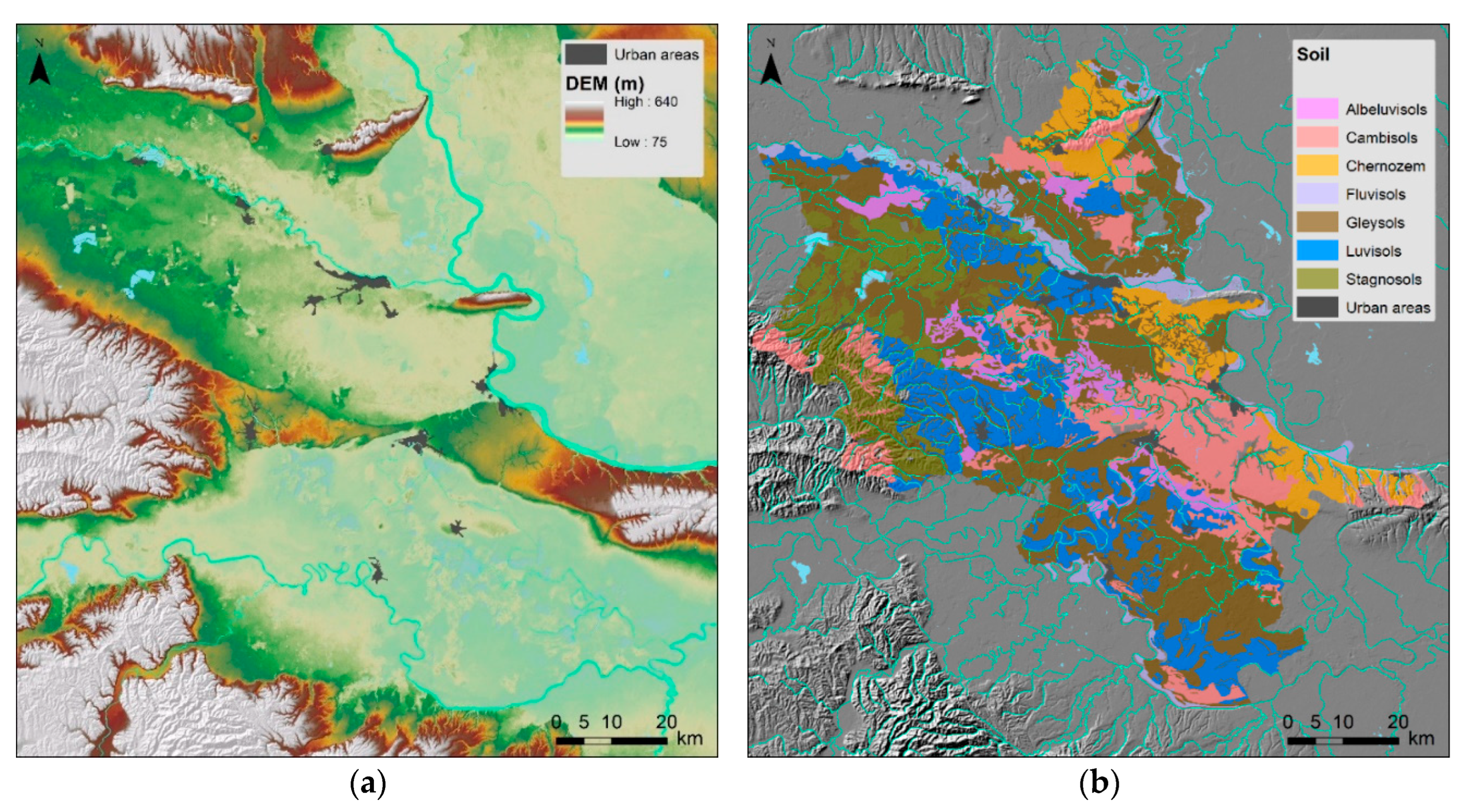
2.1. Study Site
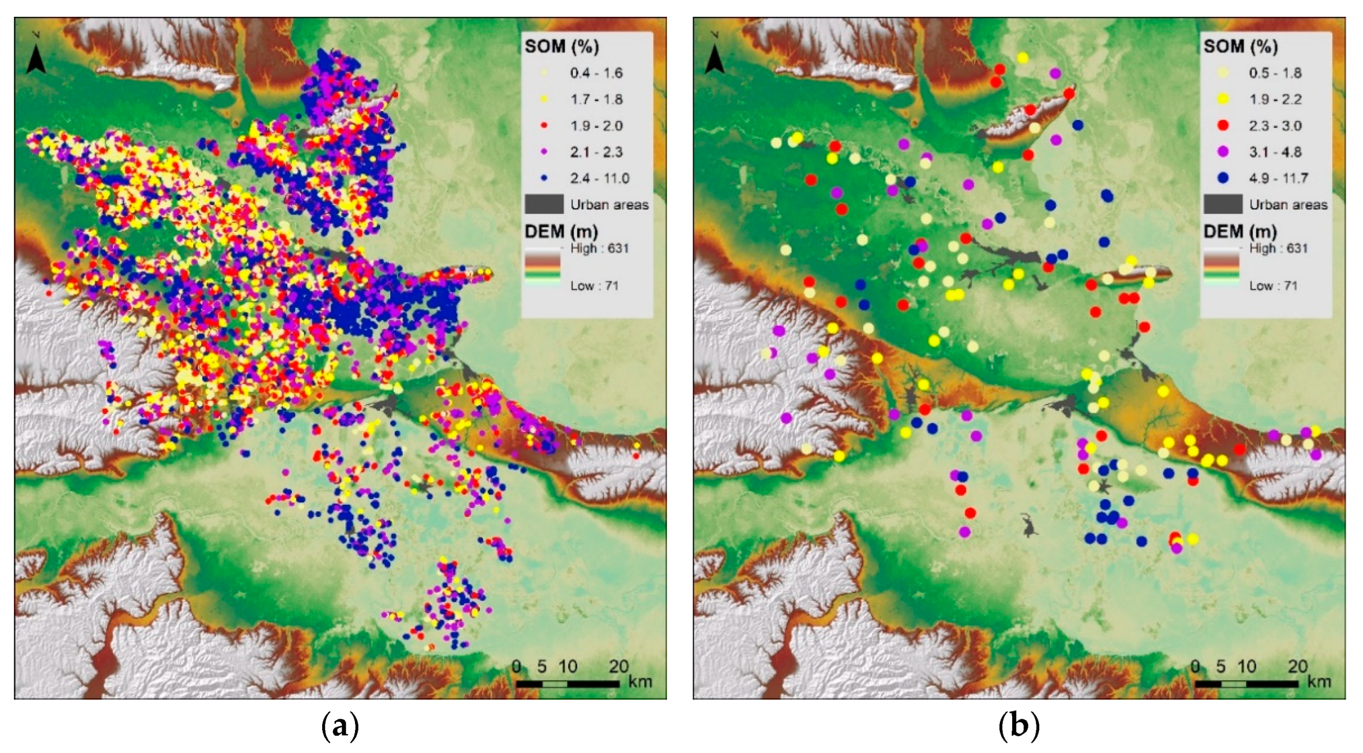
2.2. Soil Data Sets
2.2.1. SOM2010
2.2.2. SOM1970
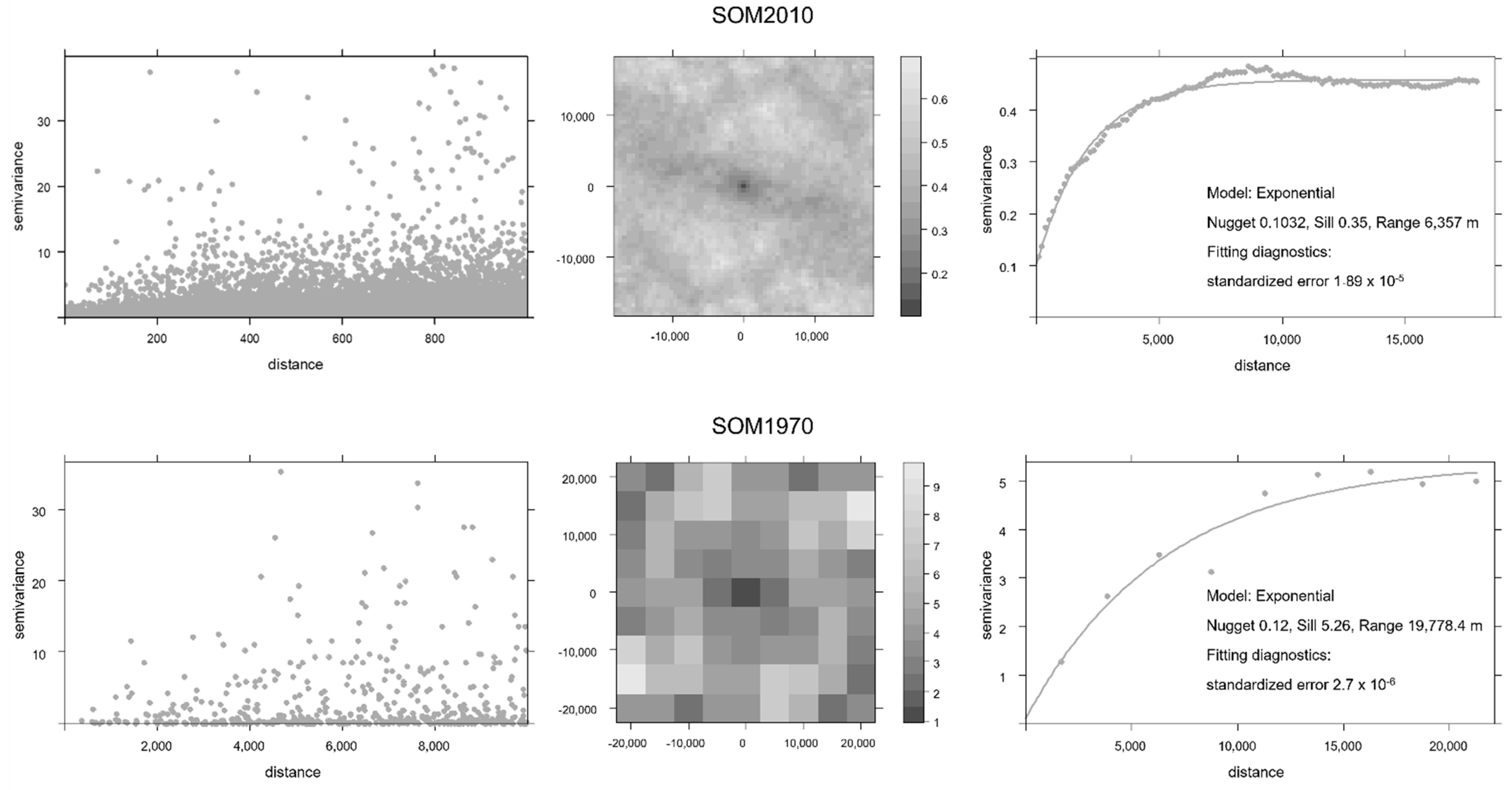
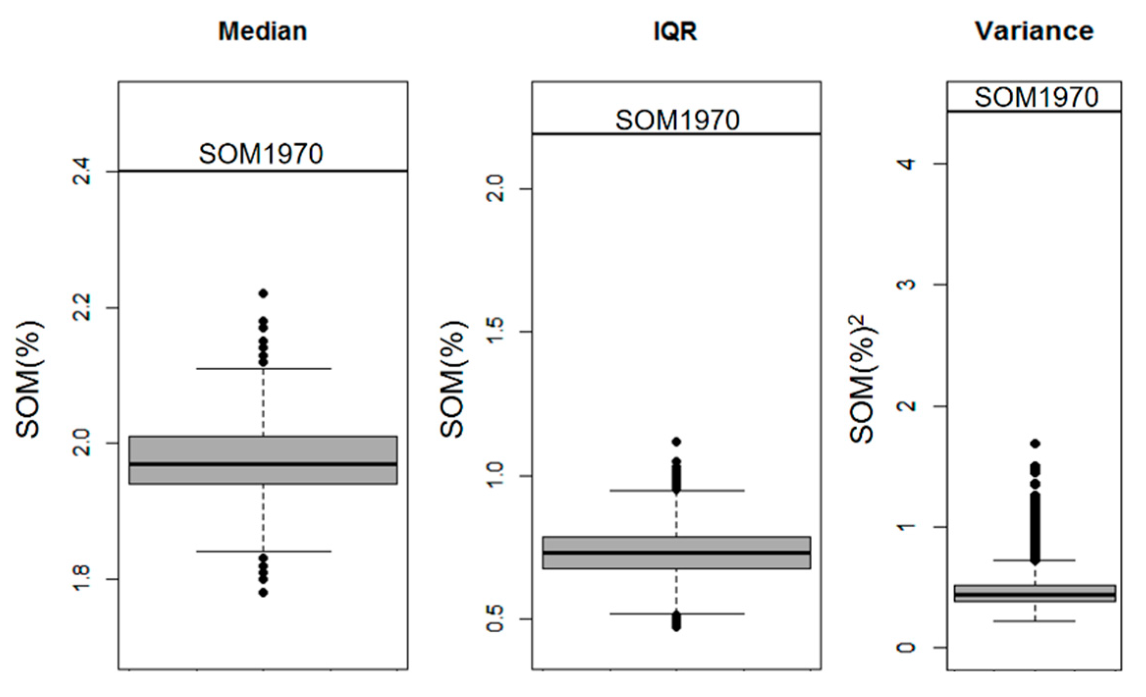
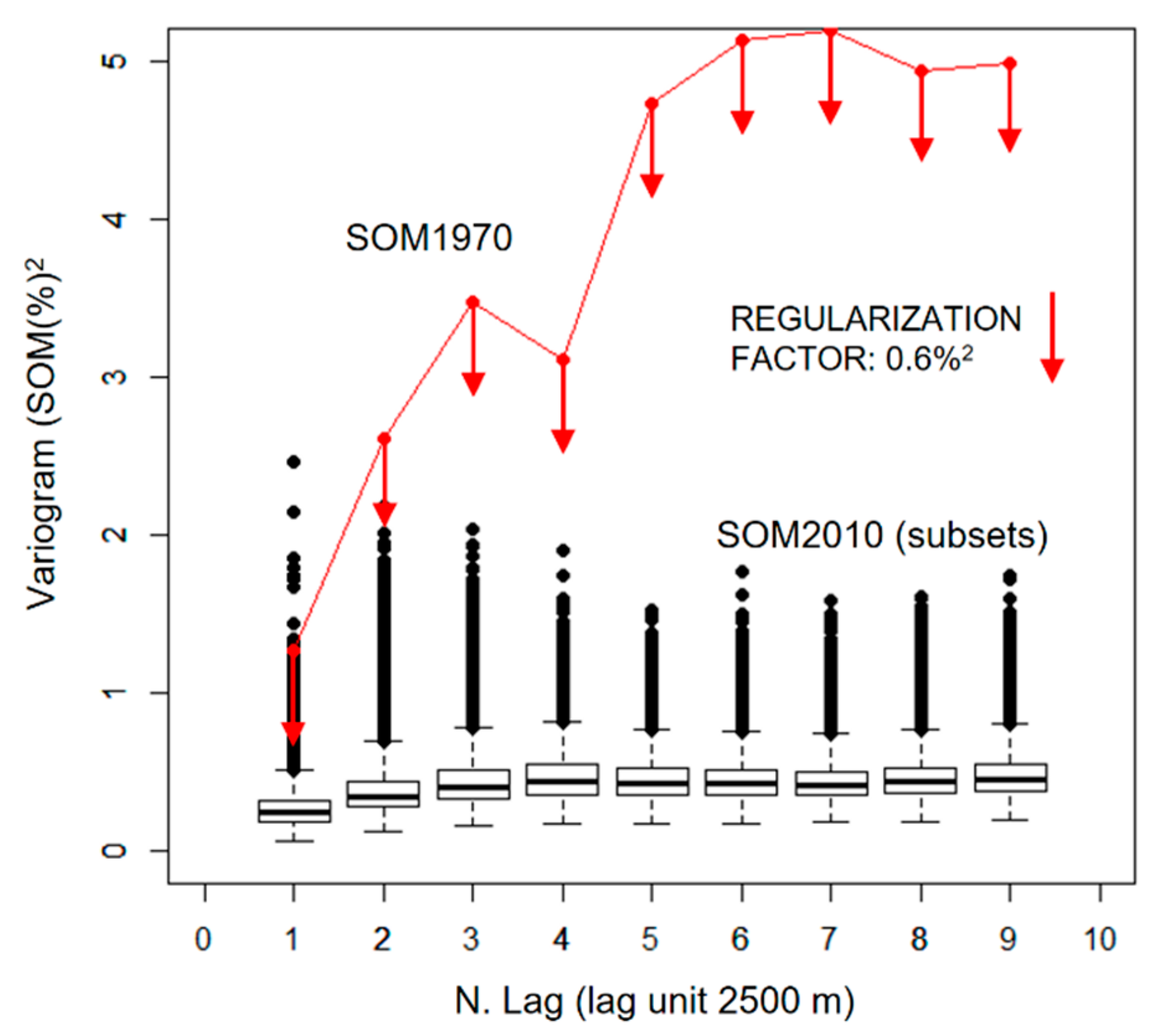
2.3. Geostatistical Analysis and Mapping
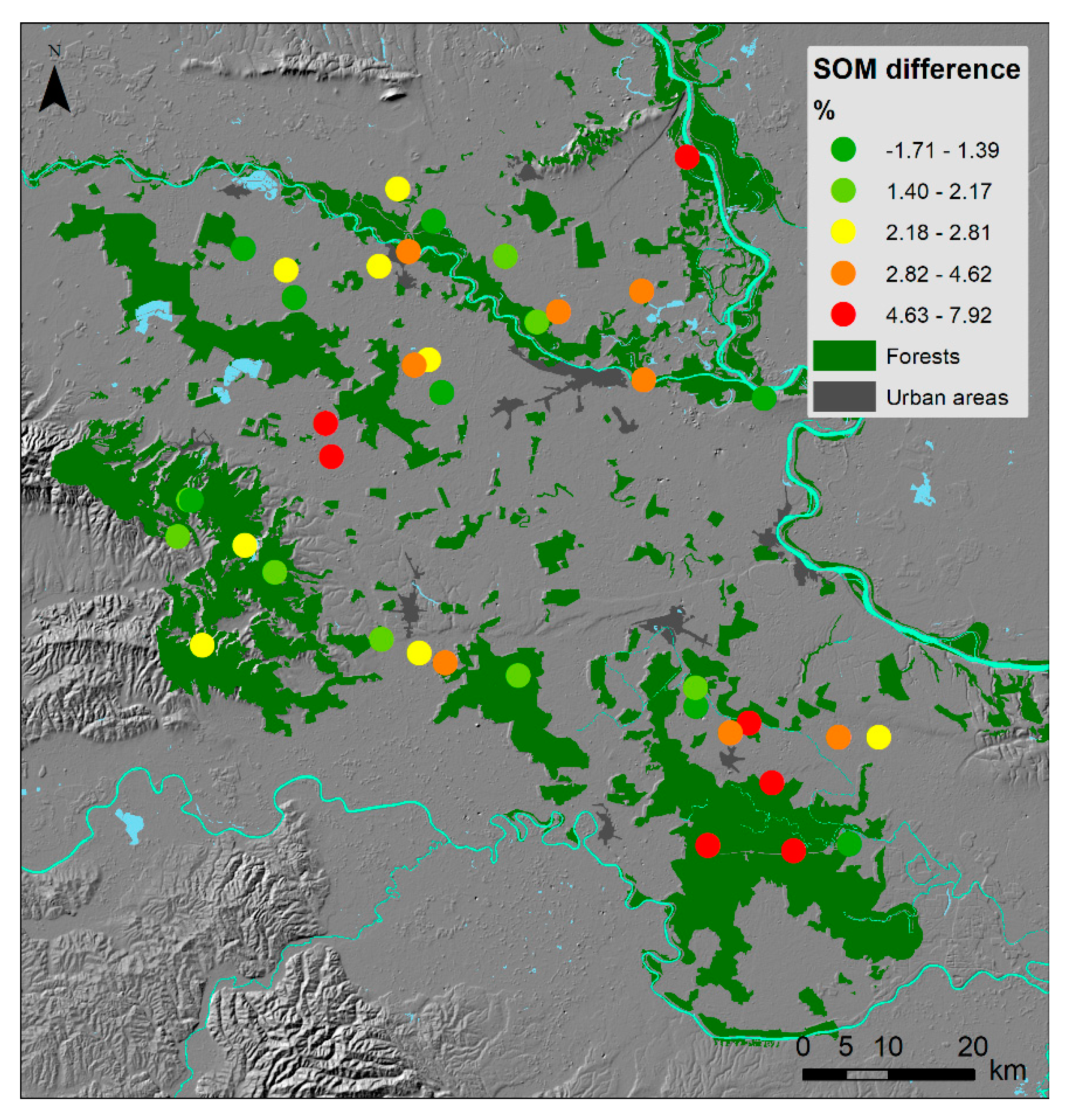
2.4. Comparison between SOM2010 and SOM1970 Datasets
3. Results and Discussion
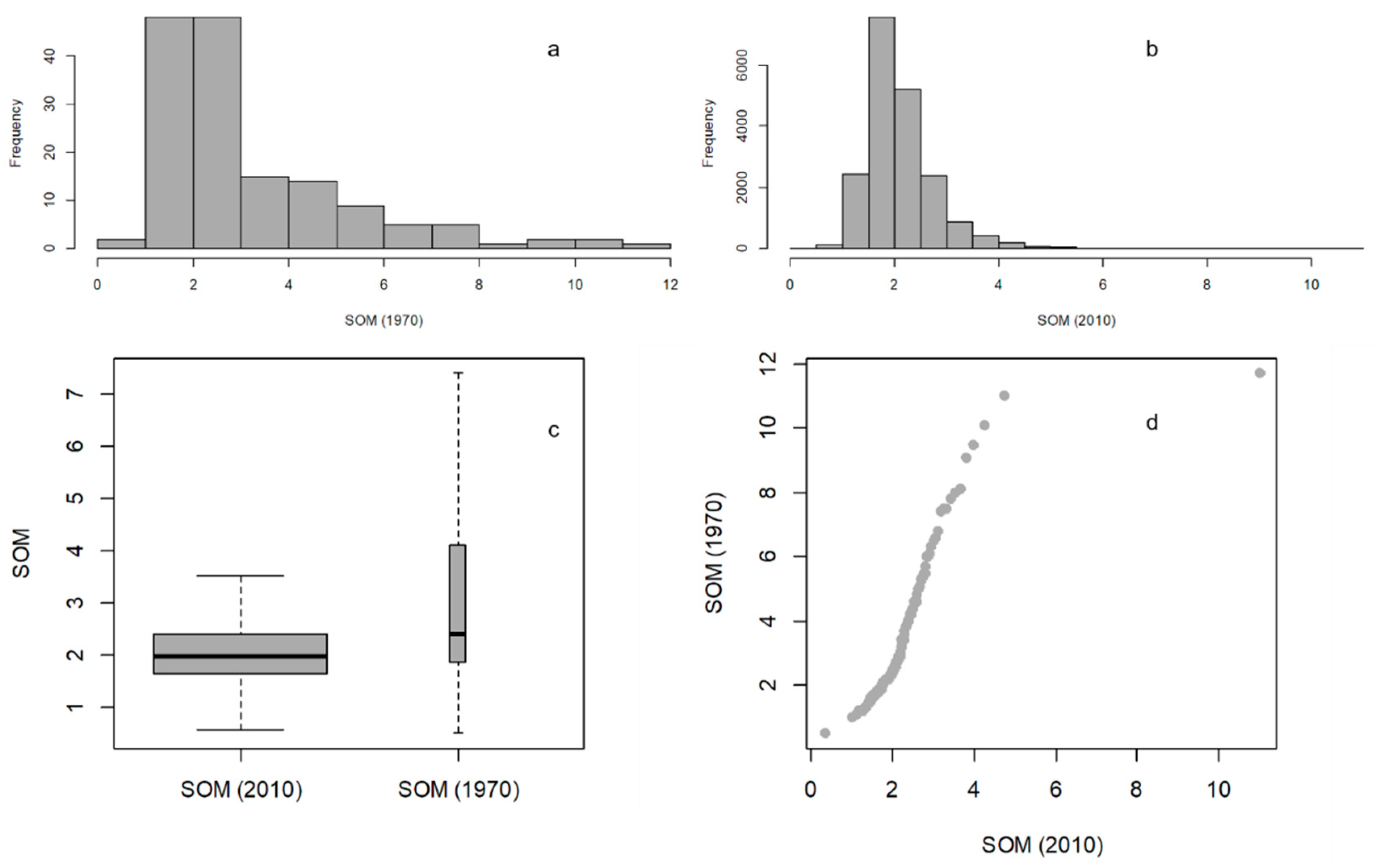
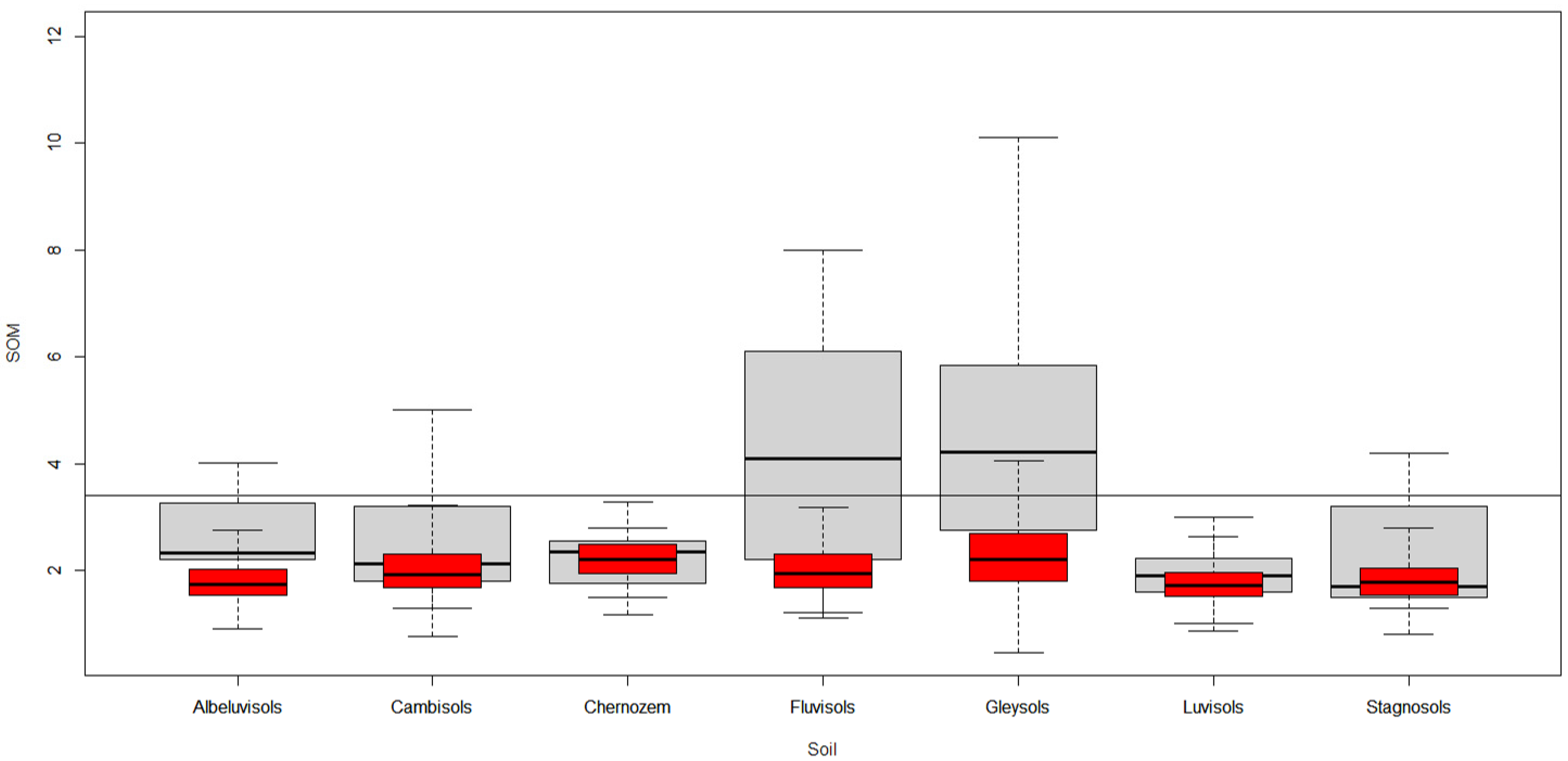
3.1. SOM Content
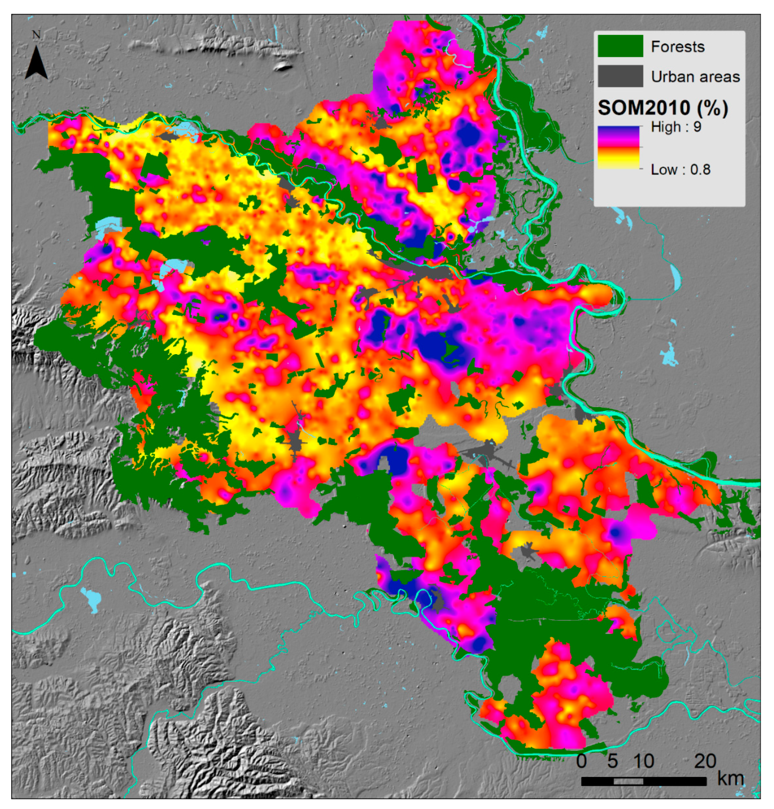
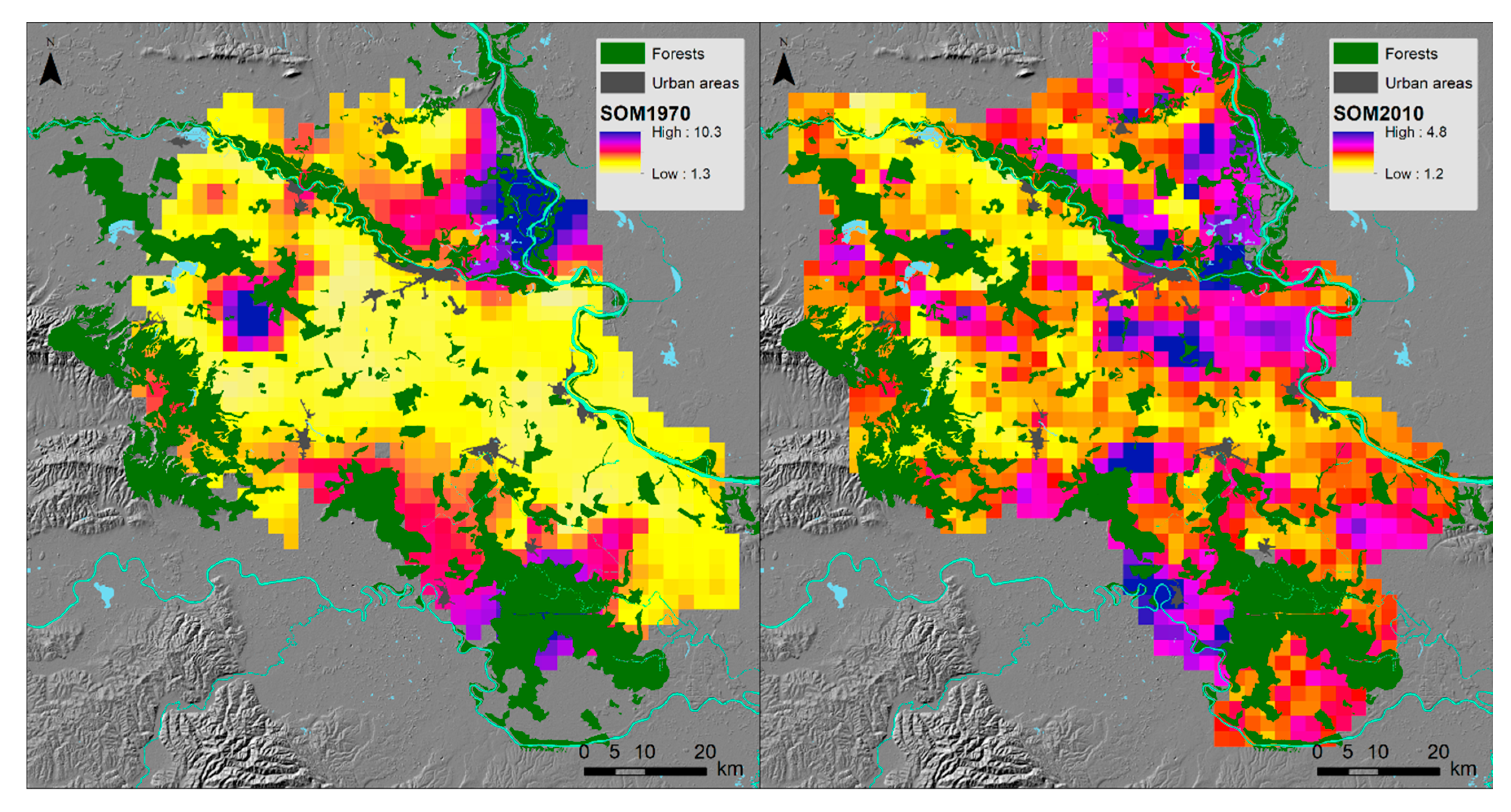
3.2. Mapping SOM2010 and SOM1970
4. Conclusions
Author Contributions
Funding
Institutional Review Board Statement
Informed Consent Statement
Data Availability Statement
Acknowledgments
Conflicts of Interest
References
- FAO. Healthy Soils Are the Basis for Healthy Food Production; Food and Agriculture Organization of the United Nations: Rome, Italy, 2015; Available online: http://www.fao.org/3/a-i4405e.pdf (accessed on 14 September 2021).
- Van de Broek, M.; Henriksen, C.B.; Ghaley, B.B.; Lugato, E.; Kuzmanovski, V.; Trajanov, A.; Debeljak, M.; Sandén, T.; Spiegel, H.; Decock, C.; et al. Assessing the climate regulation potential of Agricultural soils using a decision support tool adapted to stakeholders’ needs and possibilities. Front. Environ. Sci. 2019, 7, 131. [Google Scholar] [CrossRef] [Green Version]
- FAO; ITPS. Status of the World’s Soil Resources (Main Report); No. 608; Food and Agriculture Organization of the United Nations: Rome, Italy, 2015. [Google Scholar]
- Pacheco, F.A.L.; Fernandes, L.F.S.; Junior, R.F.V.; Valera, C.A.; Pissarra, T.C.T. Land degradation: Multiple environmental consequences and routes to neutrality. Curr. Opin. Environ. Sci. Health 2018, 5, 79–86. [Google Scholar] [CrossRef]
- Bogunovic, I.; Trevisani, S.; Pereira, P.; Vukadinovic, V. Mapping soil organic matter in the Baranja region (Croatia): Geological and anthropic forcing parameters. Sci. Total Environ. 2018, 643, 335–345. [Google Scholar] [CrossRef]
- Piikki, K.; Söderström, M. Digital soil mapping of arable land in Sweden–Validation of performance at multiple scales. Geoderma 2019, 352, 342–350. [Google Scholar] [CrossRef]
- Behera, S.K.; Mathur, R.K.; Shukla, A.K.; Suresh, K.; Prakash, C. Spatial variability of soil properties and delineation of soil management zones of oil palm plantations grown in a hot and humid tropical region of southern India. Catena 2018, 165, 251–259. [Google Scholar] [CrossRef]
- Li, X.; Shao, M.A.; Zhao, C.; Liu, T.; Jia, X.; Ma, C. Regional spatial variability of root-zone soil moisture in arid regions and the driving factors—A case study of Xinjiang, China. Can. J. Soil Sci. 2019, 99, 277–291. [Google Scholar] [CrossRef]
- Schillaci, C.; Acutis, M.; Lombardo, L.; Lipani, A.; Fantappie, M.; Märker, M.; Saia, S. Spatio-temporal topsoil organic carbon mapping of a semi-arid Mediterranean region: The role of land use, soil texture, topographic indices and the influence of remote sensing data to modelling. Sci. Total Environ. 2017, 601, 821–832. [Google Scholar] [CrossRef]
- He, S.; Zhu, H.; Shahtahmassebi, A.R.; Qiu, L.; Wu, C.; Shen, Z.; Wang, K. Spatiotemporal variability of soil nitrogen in relation to environmental factors in a low hilly region of southeastern China. Int. J. Environ. Res. Public Health 2018, 15, 2113. [Google Scholar] [CrossRef] [Green Version]
- Li, C.; Sanchez, G.M.; Wu, Z.; Cheng, J.; Zhang, S.; Wang, Q.; Li, F.; Sun, G.; Meentemeyer, R.K. Spatiotemporal patterns and drivers of soil contamination with heavy metals during an intensive urbanization period (1989–2018) in southern China. Environ. Pollut. 2020, 260, 114075. [Google Scholar] [CrossRef]
- Trevisani, S.; Omodeo, P.D. Earth Scientists and Sustainable Development: Geocomputing, New Technologies, and the Humanities. Land 2021, 10, 294. [Google Scholar] [CrossRef]
- Bogunovic, I.; Trevisani, S.; Seput, M.; Juzbasic, D.; Durdevic, B. Short-range and regional spatial variability of soil chemical properties in an agro-ecosystem in eastern Croatia. Catena 2017, 154, 50–62. [Google Scholar] [CrossRef]
- Bai, Y.; Zhou, Y. The main factors controlling spatial variability of soil organic carbon in a small karst watershed, Guizhou Province, China. Geoderma 2020, 357, 113938. [Google Scholar] [CrossRef]
- Owusu, S.; Yigini, Y.; Olmedo, G.F.; Omuto, C.T. Spatial prediction of soil organic carbon stocks in Ghana using legacy data. Geoderma 2020, 360, 114008. [Google Scholar] [CrossRef]
- Zhao, Z.; Yang, Q.; Sun, D.; Ding, X.; Meng, F.R. Extended model prediction of high-resolution soil organic matter over a large area using limited number of field samples. Comput. Electron. Agric. 2020, 169, 105172. [Google Scholar] [CrossRef]
- Jin, X.; Song, K.; Du, J.; Liu, H.; Wen, Z. Comparison of different satellite bands and vegetation indices for estimation of soil organic matter based on simulated spectral configuration. Agric. For. Meteorol. 2017, 244, 57–71. [Google Scholar] [CrossRef]
- Meng, X.; Bao, Y.; Liu, J.; Liu, H.; Zhang, X.; Zhang, Y.; Wang, P.; Tang, H.; Kong, F. Regional soil organic carbon prediction model based on a discrete wavelet analysis of hyperspectral satellite data. Int. J. Appl. Earth Obs. Geoinf. 2020, 89, 102111. [Google Scholar] [CrossRef]
- Venter, Z.S.; Hawkins, H.J.; Cramer, M.D.; Mills, A.J. Mapping soil organic carbon stocks and trends with satellite-driven high resolution maps over South Africa. Sci. Total Environ. 2021, 771, 145384. [Google Scholar] [CrossRef]
- Dugan, I.; Pereira, P.; Barcelo, D.; Telak, L.J.; Filipovic, V.; Filipovic, L.; Kisic, I.; Bogunovic, I. Agriculture management and seasonal impact on soil properties, water, sediment and chemicals transport in hazelnut orchard (Croatia). Sci. Total Environ. 2022, 839, 156346. [Google Scholar] [CrossRef]
- Diodato, N.; Bellocchi, G.; Bertolin, C.; Camuffo, D. Climate variability analysis of winter temperatures in the central Mediterranean since 1500 AD. Theor. Appl. Climatol. 2014, 116, 203–210. [Google Scholar] [CrossRef]
- Hartemink, A.E.; Krasilnikov, P.; Bockheim, J.G. Soil maps of the world. Geoderma 2013, 207, 256–267. [Google Scholar] [CrossRef]
- Brevik, E.C.; Calzolari, C.; Miller, B.A.; Pereira, P.; Kabala, C.; Baumgarten, A.; Jordán, A. Soil mapping, classification, and pedologic modeling: History and future directions. Geoderma 2016, 264, 256–274. [Google Scholar] [CrossRef]
- Camuffo, D.; Bertolin, C.; Schenal, P. A novel proxy and the sea level rise in Venice, Italy, from 1350 to 2014. Clim. Chang. 2017, 143, 73–86. [Google Scholar] [CrossRef]
- Bogunovic, I.; Kisic, I. Compaction of a Clay Loam Soil in Pannonian Region of Croatia under Different Tillage Systems. J. Agric. Sci. Technol. 2017, 19, 475–486. [Google Scholar]
- Dekemati, I.; Simon, B.; Bogunovic, I.; Vinogradov, S.; Modiba, M.M.; Gyuricza, C.; Birkás, M. Three-Year Investigation of Tillage Management on the Soil Physical Environment, Earthworm Populations and Crop Yields in Croatia. Agronomy 2021, 11, 825. [Google Scholar] [CrossRef]
- Jug, D.; Đurđević, B.; Birkás, M.; Brozović, B.; Lipiec, J.; Vukadinović, V.; Jug, I. Effect of conservation tillage on crop productivity and nitrogen use efficiency. Soil Tillage Res. 2019, 194, 104327. [Google Scholar] [CrossRef]
- Bogunovic, I.; Telak, L.J.; Pereira, P. Experimental comparison of runoff generation and initial soil erosion between vineyards and croplands of Eastern Croatia: A case study. Air Soil Water Res. 2020, 13, 1178622120928323. [Google Scholar] [CrossRef]
- Telak, L.J.; Bogunovic, I. Tillage-induced impacts on the soil properties, soil water erosion, and loss of nutrients in the vineyard (Central Croatia). J. Cent. Eur. Agric. 2020, 21, 589–601. [Google Scholar] [CrossRef]
- Telak, L.J.; Dugan, I.; Bogunovic, I. Soil Management and Slope Impacts on Soil Properties, Hydrological Response, and Erosion in Hazelnut Orchard. Soil Syst. 2021, 5, 5. [Google Scholar] [CrossRef]
- Loveland, P.; Webb, J. Is there a critical level of organic matter in the agricultural soils of temperate regions: A review. Soil Tillage Res. 2003, 70, 1–18. [Google Scholar] [CrossRef]
- Lehmann, J.; Kleber, M. The contentious nature of soil organic matter. Nature 2015, 528, 60–68. [Google Scholar] [CrossRef] [PubMed]
- Murphy, B.W. Impact of soil organic matter on soil properties—A review with emphasis on Australian soils. Soil Res. 2015, 53, 605–635. [Google Scholar] [CrossRef]
- Ács, F. On Twenty-First Century Climate Classification: European Multiregional Analyses; LAP Lambert Academic Publishing: Beau Bassin, Mauritius, 2017. [Google Scholar]
- Zaninović, K.; Gajić-Čapka, M.; Perčec Tadić, M.; Vučetić, M.; Milković, J.; Bajić, A.; Cindrić, K.; Cvitan, L.; Katušin, Z.; Kaučić, D.; et al. Climate Atlas of Croatia: 1961–1990, 1971–2000; Croatian Meteorological and Hydrological Service: Zagreb, Croatia, 2008. [Google Scholar]
- Škorić, A.; Anić, J.; Beštak, T.; Bišof, R.; Bogunović, M.; Cestar, D.; Čižek, J.; Dekanić, I.; Kovačević, J.; Licul, R.; et al. Soils of Slavonia and Baranja; Projektni Savjet Pedološke Karte SR Hrvatske: Zagreb, Croatia, 1977. (In Croatian) [Google Scholar]
- Bačani, A.; Šparica, M.; Velić, J. Quaternary deposits as the hydrogeological system of Eastern Slavonia. Geol. Croat. 1999, 52, 141–152. [Google Scholar]
- Velić, I.; Vlahović, I. Geological Map of the Republic of Croatia 1: 300.000; Croatian Geological Survey: Zagreb, Croatia, 2009. [Google Scholar]
- Bašić, F. The Soils of Croatia; Springer: Dordrecht, The Netherlands; Heidelberg, Germany; New York, NY, USA; London, UK, 2013. [Google Scholar]
- IUSS Working Group WRB. World Reference Base for Soil Resources 2014, Update 2015: International Soil Classification System for Naming Soils and Creating Legends for Soil Maps; World Soil Resources Reports No. 106; FAO: Rome, Italy, 2015; pp. 150–200. [Google Scholar]
- Isaaks, E.H.; Srivastava, R.M. Applied Geostatistics; Oxford University: London, UK, 1989. [Google Scholar]
- Nelson, D.W.; Sommers, L.E. Total carbon, organic carbon, and organic matter. Part II. Chemical and Microbiological Properties. In Methods of Soil Analysis, 2nd ed.; Page, A.L., Miller, R.H., Keeney, D.R., Eds.; American Society of Agronomy: Madison, WI, USA, 1982; pp. 539–579. [Google Scholar]
- Bogunović, M.; Vidaček, Ž.; Husnjak, S.; Sraka, M. Inventory of soils in Croatia. Agric. Conspec. Sci. 1998, 63, 105–112. [Google Scholar]
- Pansu, M.; Gautheyrou, J. Handbook of Soil Analysis: Mineralogical, Organic and Inorganic Methods; Springer Science & Business Media: Berlin/Heidelberg, Germany, 2007. [Google Scholar] [CrossRef]
- Hengl, T.; MacMillan, R.A. Predictive Soil Mapping with R; OpenGeoHub Foundation: Wageningen, The Netherlands, 2019; Available online: https://soilmapper.org/PSMwR_lulu.pdf (accessed on 16 November 2021).
- Pebesma, E.J. Multivariable geostatistics in S: The gstat package. Comput. Geosci. 2004, 30, 683–691. [Google Scholar] [CrossRef]
- Ploner, A. The use of the variogram cloud in geostatistical modelling. Environmetrics 1999, 10, 413–437. [Google Scholar] [CrossRef]
- Hengl, T.; Heuvelink, G.B.; Stein, A. A generic framework for spatial prediction of soil variables based on regression-kriging. Geoderma 2004, 120, 75–93. [Google Scholar] [CrossRef] [Green Version]
- Goovaerts, P. Geostatistical tools for characterizing the spatial variability of microbiological and physico-chemical soil properties. Biol. Fertil. Soils 1998, 27, 315–334. [Google Scholar] [CrossRef] [Green Version]
- Hastie, T.; Tibshirani, R.; Friedman, J. The Elements of Statistical Learning: Data Mining, Inference, and Prediction, 2nd ed.; Springer: New York, NY, USA, 2009. [Google Scholar]
- Atkinson, P.M. Regularizing Variograms of Airborne MSS Imagery. Can. J. Remote Sens. J. 1995, 21, 225–233. [Google Scholar] [CrossRef]
- Körschens, M.; Albert, E.; Armbruster, M.; Barkusky, D.; Baumecker, M.; Behle-Schalk, L.; Bischoff, R.; Čergan, Z.; Ellmer, F.; Herbst, F.; et al. Effect of mineral and organic fertilization on crop yield, nitrogen uptake, carbon and nitrogen balances, as well as soil organic carbon content and dynamics: Results from 20 European long-term field experiments of the twenty-first century. Arch. Agron. Soil Sci. 2013, 59, 1017–1040. [Google Scholar] [CrossRef]
- Bogunovic, I.; Filipovic, L.; Filipovic, V.; Kisic, I. Agricultural Land Degradation in Croatia. In Impact of Agriculture on Soil Degradation I—A European Perspective , 1st ed.; The Handbook of Environmental, Chemistry; Pereira, P., Muñoz-Rojas, M., Bogunovic, I., Zhao, W., Eds.; Springer: Cham, Switzerland, 2022; in press. [Google Scholar]
- Telak, L.J.; Pereira, P.; Bogunovic, I. Management and seasonal impacts on vineyard soil properties and the hydrological response in continental Croatia. Catena 2021, 202, 105267. [Google Scholar] [CrossRef]
- Bogunovic, I.; Pereira, P.; Kisic, I.; Sajko, K.; Sraka, M. Tillage management impacts on soil compaction, erosion and crop yield in Stagnosols (Croatia). Catena 2018, 160, 376–384. [Google Scholar] [CrossRef]
- Filipovic, D.; Husnjak, S.; Kosutic, S.; Gospodaric, Z. Effects of tillage systems on compaction and crop yield of Albic Luvisol in Croatia. J. Terramech. 2006, 43, 177–189. [Google Scholar] [CrossRef]
- Baltruschat, H.; Santos, V.M.; da Silva, D.K.A.; Schellenberg, I.; Deubel, A.; Sieverding, E.; Oehl, F. Unexpectedly high diversity of arbuscular mycorrhizal fungi in fertile Chernozem croplands in Central Europe. Catena 2019, 182, 104135. [Google Scholar] [CrossRef]
- Husnjak, S. Sistematika Tala Hrvatske; Hrvatska Sveučilišna Naklada: Zagreb, Croatia, 2014. (In Croatian) [Google Scholar]
- Teklić, T.; Vukadinović, V.; Lončarić, Z.; Rengel, Z.; Dropulić, D. Model for optimizing fertilization of sugar beet, wheat, and maize grown on Pseudogley soils. J. Plant Nutr. 2002, 25, 1863–1879. [Google Scholar] [CrossRef]
- Žimbrek, T. Consultancy services in Croatian agriculture. Agric. Conspec. Sci. 1997, 62, 267–274. [Google Scholar]
- Croatian Bureau of Statistics. Census of Agriculture 1969. Available online: http://www.popispoljoprivrede.hr/povijest.html (accessed on 1 February 2022).
- Eurostat. Eurostat Regional Yearbook 2013. European Commission. 2013. Available online: https://ec.europa.eu/eurostat/documents/3217494/5784301/KS-HA-13-001-EN.PDF (accessed on 1 February 2022).
- Machmuller, M.B.; Kramer, M.G.; Cyle, T.K.; Hill, N.; Hancock, D.; Thompson, A. Emerging land use practices rapidly increase soil organic matter. Nat. Commun. 2015, 6, 6995. [Google Scholar] [CrossRef]
- Wang, X. Changes in Cultivated Land Loss and Landscape Fragmentation in China from 2000 to 2020. Land 2022, 11, 684. [Google Scholar] [CrossRef]
- Birkás, M.; Szemők, A.; Antos, G.; Neményi, M. Environmentally-Sound Adaptable Tillage; Akadémiai Kiadó: Budapest, Hungary, 2008. [Google Scholar]
- Balesdent, J.; Chenu, C.; Balabane, M. Relationship of soil organic matter dynamics to physical protection and tillage. Soil Tillage Res. 2000, 53, 215–230. [Google Scholar] [CrossRef]


| Dataset | n | Spatial Spacing (m) | Min | 1st Quartile | Median | Mean | 3rd Quartile | Max | |
|---|---|---|---|---|---|---|---|---|---|
| Mean | Median | ||||||||
| SOM1970 | 152 | 2595.6 | 2955.4 | 0.50 | 1.87 | 2.40 | 3.25 a | 4.07 | 11.70 |
| SOM2010 | 19,386 | 147 | 164 | 0.32 | 1.66 | 1.97 | 2.11 b | 2.40 | 11.00 |
| SOM2010 | SOM1970 | |||
|---|---|---|---|---|
| Error | Absolute Error | Error | Absolute Error | |
| RMSE | 0.41 | 1.66 | ||
| RMSSE | 1.03 | 1.06 | ||
| Minimum | −8.30 | 0.0 | −5.63 | 0.02 |
| 1st Qu. | −0.16 | 0.08 | −0.68 | 0.29 |
| Median | 0.03 | 0.19 | 0.18 | 0.84 |
| Mean | 0.0 | 0.27 | 0.0 | 1.22 |
| 3rd Qu. | 0.21 | 0.35 | 0.85 | 1.82 |
| Maximum | 6.10 | 8.30 | 4.47 | 5.63 |
Publisher’s Note: MDPI stays neutral with regard to jurisdictional claims in published maps and institutional affiliations. |
© 2022 by the authors. Licensee MDPI, Basel, Switzerland. This article is an open access article distributed under the terms and conditions of the Creative Commons Attribution (CC BY) license (https://creativecommons.org/licenses/by/4.0/).
Share and Cite
Trevisani, S.; Bogunovic, I. Diachronic Mapping of Soil Organic Matter in Eastern Croatia Croplands. Land 2022, 11, 861. https://doi.org/10.3390/land11060861
Trevisani S, Bogunovic I. Diachronic Mapping of Soil Organic Matter in Eastern Croatia Croplands. Land. 2022; 11(6):861. https://doi.org/10.3390/land11060861
Chicago/Turabian StyleTrevisani, Sebastiano, and Igor Bogunovic. 2022. "Diachronic Mapping of Soil Organic Matter in Eastern Croatia Croplands" Land 11, no. 6: 861. https://doi.org/10.3390/land11060861
APA StyleTrevisani, S., & Bogunovic, I. (2022). Diachronic Mapping of Soil Organic Matter in Eastern Croatia Croplands. Land, 11(6), 861. https://doi.org/10.3390/land11060861