Article

Predictive Mapping of Electrical Conductivity and Assessment of Soil Salinity in a Western Türkiye Alluvial Plain

1
Department of Soil Science and Plant Nutrition, Faculty of Agriculture, Isparta University of Applied Sciences, Isparta 32260, Türkiye
2
European Commission, Joint Research Centre, Via E. Fermi, 2749, 21027 Ispra, VA, Italy
3
Laboratory of Remote Sensing and GIS, Department of Soil Science, University of Tehran, P.O. Box 4111, Karaj 31587-77871, Iran
*
Author to whom correspondence should be addressed.
Land 2022, 11(12), 2148; https://doi.org/10.3390/land11122148
Submission received: 30 September 2022 / Revised: 9 November 2022 / Accepted: 25 November 2022 / Published: 28 November 2022

Abstract

:
The increase in soil salinity due to human-induced processes poses a severe threat to agriculture on a regional and global scale. Soil salinization caused by natural and anthropogenic factors is a vital environmental hazard, specifically in semi-arid and arid regions of the world. The detection and monitoring of salinity are critical to the sustainability of soil management. The current study compared the performance of machine learning models to produce spatial maps of electrical conductivity (EC) (as a proxy for salinity) in an alluvial irrigation plain. The current study area is located in the Isparta province (100 km2), land cover is mainly irrigated, and the dominant soils are Inceptisols, Mollisols, and Vertisols. Digital soil mapping (DSM) methodology was used, referring to the increase in the digital representation of soil formation factors with today’s technological advances. Plant and soil-based indices produced from the Sentinel 2A satellite image, topographic indices derived from the digital elevation model (DEM), and CORINE land cover classes were used as predictors. The support vector regression (SVR) algorithm revealed the best relationships in the study area. Considering the estimates of different algorithms, according to the FAO salinity classification, a minimum of 12.36% and a maximum of 20.19% of the study area can be classified as slightly saline. The low spatial dependence between model residuals limited the success of hybrid methods. The land irrigated cover played a significant role in predicting the current level of EC.

1. Introduction

The increase in soil salinity seriously threatens agriculture on a regional and global scale [1]. Soil salinization caused by natural and anthropogenic factors is an essential environmental hazard, especially in arid and semi-arid regions of the world. There is a consensus on the need for the most accurate determination and monitoring of soil information to support sustainable development within the goals specified by the Sustainable Development Goals (SDGs) [2].
In soil salinization, a distinction is made between the primary (natural) and secondary (human-induced) processes [3,4,5]. In the primary formation process, salinization is associated with natural climatic conditions such as a lack of precipitation and an excess of evapotranspiration in semi-arid and arid climates and with the parent geological material [6,7]. The secondary process is caused by human activities such as irrigation and poor drainage conditions using low-quality irrigation waters [8]. The characteristic cause of soil salinization relies on the local soil properties of the area and the topography that plays an active role in groundwater transport processes. These factors vary with climate, land cover, different agricultural activities, different irrigation methods, and related soil and water management practices [9,10]. As a result of irresponsible irrigation and low-quality irrigation waters, capillarity, the soil dynamic system, is prone to increasing soil salinity on the soil surface in arid and semi-arid regions [5].
The rise in the frequency of adverse climatic conditions, such as higher temperatures in summer and changes in precipitation patterns, increased irrigated land to meet the food demand, especially in Mediterranean regions with arid and semi-arid climates [11,12]. The combination of the high water-consuming conventional irrigation methods and inadequate drainage systems will potentially increase soil salinity problems in many arable lands with climate change on a global scale [13,14,15].
Irrigation in arid and semi-arid areas is crucial to sustaining agricultural production [16]. In the irrigated areas of semi-arid regions, monitoring soil salinity [17,18] is extremely important to avoid loss of yields and increase degradation processes that can turn fertile land into badlands in the short term. The soil science community have been interested in producing the most accurate spatial information on the current state of soil salinity to warn policy stakeholders that in the near future, irrigated agricultural activities might suffer from salinity and therefore not be so adapted for food production. At a global scale, studies have been carried out to guide the management of saline soils better, e.g., the FAO’s new GSAS (Global Map of Salt-Affected Soils) map v1.0 is a forefront partnership to foster research on salinity, identifying salt-affected areas and where sustainable soil management practices should be adopted [19].
The fact that spatial representation in a digital form of the soil-forming factors has become probable makes the DSM framework effectively usable [20]. The relationship of socio-ecological differences with irrigation and using land cover classes as a covariate [21] is being investigated [22]. Furthermore, multispectral satellite images with higher spatial resolution are used for cost-effective detection and monitoring of the current state of soil salinity [23]. It is important to know two distinctions regarding remote sensing (RS) products. Firstly, direct methods can be used in studies to detect and monitor the primary salinization process based on the reflective properties of salts and crusts on the bare soil surface [24]. Secondly, areas with and without salt on the bare soil surface can be discriminated due to the high reflectivity of the salt-covered regions in the visible region of the electromagnetic spectrum.
However, direct methods are less useful in agricultural areas due to different land cover types. Therefore, the focus is on indirect RS methods for soil salinity monitoring [5]. Indirect methods such as canopy spectral reflectance can often determine root zone salinity based on plant growth and health. The visible or infrared spectra reflection usually differs for healthy and salt-stressed plants. Regression-based machine learning models can be utilized to predict soil salinity levels from remote sensing imagery if a relationship can be established between the soil surface EC and the spectral response [5].
Land use/land cover (LULC) maps are critical geospatial data decision makers needed to monitor environmental change at a regional or global scale and quantify the risk to sustainable livelihoods and development [25]. These data can be used as environmental variables in detecting and monitoring the current state of dynamic soil properties in DSM processes [3,22,26]. Land cover/use information can represent biotic and anthropogenic activities and the driving forces that are effective in the formation of salinization in the soil due to a secondary (human-induced) process [3]. Integrated with remote sensing land cover classes, DSM can provide valuable insights to produce maps of soil salinity and track changes in soil salinity over time [27]. Land cover data must be known over a long period to be used as an environmental variable. The availability of spatial data based on such a long observation reduces the potential to underestimate the spatial variability of the salinity under the categories [28].
Accurate and reliable case-based DSM mapping studies have been performed using various combinations of soil formation factors for a quarter of a century, using multiple machine learning techniques within the framework of DSM [29]. Maleki et al. [30] used a random forest (RF) model within the framework of DSM to examine the spatial–temporal change processes in soil salinity and alkalinity. They determined groundwater properties, urban structure, and distance from the road as the most influential environmental variables. Naimi et al. [31] compared the effectiveness of different machine learning algorithms and environmental covariate scenarios to predict spatial soil salinity by deriving information from RS data, DEM, and proximal sensing (PS). They reported the best estimation accuracy for the RF model in the scenario using all environmental variables. In addition, they said that topography as an environmental variable is of great importance in their study. Furthermore, Zhao et al. [32] reported the successful integration of soil properties, such as exchangeable cations and cation exchange capacity [33] as well as soil particle fractions [34], which may be related to electrical conductivity at different depths, into digital soil mapping methodology by utilizing proximal sensing techniques.
Hybrid methods can significantly improve modelling results when model residuals show moderate or spatial solid autocorrelation [35]. Yang et al. [36] compared the multiple linear regression (MLR) model and the regression-kriging approach and reported that the regression-kriging method, which considers the model residuals, produces more accurate model results.
In DSM studies, algorithms that have the capacity to capture linear and non-linear relationships in the study area are used comparatively, and the maps they produce are evaluated in the experience of soil scientists [37].
FAO has developed guidelines, and EC can be used as a proxy for salinity [3]. The science of digital soil mapping is in the development stage in Türkiye, where the current study is located [38,39]. Studies are rare on the prediction of salinity in areas where irrigated agriculture has been conducted for many years. However, the use of open-source CORINE data as environmental variables in EC estimation was not investigated in the country and Mediterranean biogeography of the study area. Specifically, the current study was carried out to spatially estimate salinity development in an alluvial plain where there is irrigated farming. We aimed (i) to determine the value of CORINE land cover class data, which have been open access for many years, in estimating anthropogenic salinity development, and (ii) to compare the performance of algorithms (random forests and support vector regression) based on different mathematical bases to explore the relationship between soil-forming factors and EC measurements. (iii) In line with the GIS analysis to be carried out on the obtained digital maps, we also aimed to evaluate the areas with high salinity risk at the plain scale for spatial decision support.

2. Materials and Methods
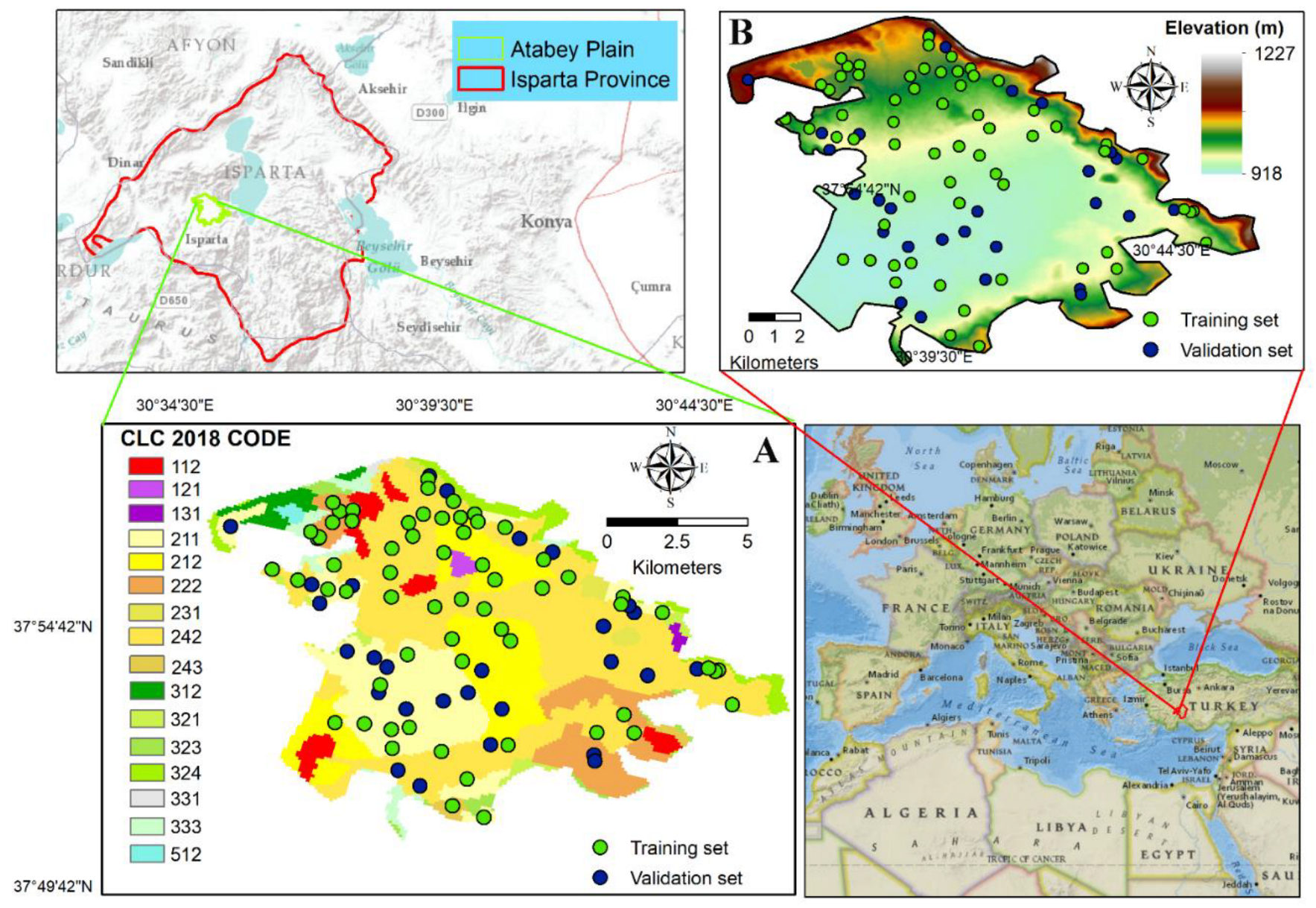
2.1. Study Area

The current study area was in the Mediterranean region in the west of Türkiye. This covers an area of about 100 km2 located between the coordinates of the World Geodetic System (WGS), bounded by latitudes 37°50′30″ and 37°58′00″ N, and longitudes 30°35′00″ and 30°46′00″ E (Figure 1). According to the Java Newhall simulation model (NSM), the study area has a xeric soil moisture regime and a mesic soil temperature regime (Supplementary Material Figure S1) [40]. The Java Newhall simulation model takes the weather stations’ monthly average temperature and precipitation data and simulates the humidity profile’s behavior [40]. Isparta Atabey plain is arable land that has been irrigated for half a century [41]. The climate type of the region is hot-summer Mediterranean (Csa) according to the Köppen–Geiger climate classification system, with an average annual temperature of 12.80 °C [42]. The mean annual rainfall and evaporation are 448.83 mm and 737.18 mm, respectively. In the study area, the central and southwest clayey soil (associated with USDA soil taxonomy Vertic Haploxerolls and Udic Haploxererts) with aged alluvial deposits are characterized by its texture. The young alluvial bed region of the study area is characterized by a partially loamy and coarser soil texture (associated with USDA soil taxonomy Typic Calcixerepts). Colluvial foothills to the east of the study area are characterized by a coarser texture [43].
According to the Newhall simulation model, an acceleration arising from soil capillarity for salinity is expected when unsuitable irrigation activities and low drainage conditions are combined in the soil’s moisture section during the irrigation period from mid-June to mid-August (Supplementary Material Figure S1).
The distribution of CORINE land cover classes (CLCC) of the current study area is given in Figure 1. Approximately 84% of the study area is arable land [44]. In this area, the crop pattern includes apple, cherry, wheat, sugar beet, walnut, and rose. The current study area consists mainly of Holocene-aged deposits. This structure is comprised of Mesozoic–Tertiary limestone surrounding the plain. Alluvial, colluvial, and fluvial deposits formed on this parent material. These coarse deposits are arranged on limestone hillslopes, surrounded by fine-structured deposits in the middle of the Atabey plain in the form of a closed bowl. In the context of geomorphology, the alluvial plain of Atabey is affected by the sediments of the Akçay River [45].

2.2. Soil Sampling and Analysis

The surface soil samples were collected from the 0–30 cm depth interval, performed using a stratified (soil series) random sampling method [46]. GPS Magellan eXplorist XL recorded coordinates for all sampling locations. Ninety-one soil samples were collected in November 2019, and EC (µS cm−1) was measured by a conductivity meter (Orion Star A112; Thermo Fisher Scientific, Waltham, MA, USA) in saturated paste [47]. In addition, the soil saturation percentage (SSP) value was recorded as the amount of water added divided by the soil weight. Soil texture analysis was carried out in the laboratory via the Bouyoucos hydrometer method, and clay (<0.002 mm), silt (0.002–0.05 mm), and sand (0.05–2 mm) were determined as percentages [48]. Cation exchange capacity (CEC) was measured with reference to the sodium acetate method [49,50]. Soil sampling locations and spatial distribution of training set (green circles) and validation set (blue circles) are shown on CORINE land cover class 2018 data in Figure 1.

2.3. Environmental Covariates

The current study’s topographic variables [51] were derived from DEM, soil and vegetation-based indices generated from Sentinel 2A-MSI satellite images, representing organisms, and parent material [52]. CORINE 2018 land cover classes [44], which can play a dominant role in explaining the variability of human impact at the regional scale in the EC, were used as environmental covariates. The DSM approach is based on the SCORPAN concept (soil, climate, organisms, topography, parent material, and spatial location) [20]. Climate variables (C), specific to the study area, are not generally used because they do not provide sufficient variations. Adequate evidence for this has been carefully presented in previous studies [53]. Our study chose not to use it due to the low variation, considering the field size.

2.3.1. Topographic Derivatives

In general, the effect of primary (basic land-surface parameters) and secondary (related to the concavity and convexity of the surface) topographic derivatives obtained from a digital elevation model on EC is well defined [54,55]. We integrated primary and secondary topographic derivatives (Table 1) into the model to evaluate this covariate’s influence on EC’s spatial distribution. The topographic features of the study area were derived for DEM resolution of 12.5 × 12.5 m (https://search.asf.alaska.edu/ (accessed on 5 September 2021)) [56]. Following Schillaci et al. [51] and Gruber and Peckham [57], terrain derivatives were calculated from the DEM and used as the covariates in the modelling process (Table 1).

2.3.2. Remote Sensing-Based Indices

Remote sensing indexes represent organism and parent material for estimating soil EC in the digital soil mapping methodology [5]. We produced the indices in Table 1, which are generally used in the literature. Sentinel 2A MSI images were obtained near the soil samples date November 2019 [58]. The Sentinel 2A MSI spectral wavelength spans from 442.7 to 2202.4 nm and spectral resolution of the bands spans from 10 to 60 m [58]. The current study used product ID: S2A_MSIL2A_20191116T085231_N0213_R107_T36STH. S2A is the mission ID, Level 2A denotes the product level, N0213 denotes the processing baseline number, and R107 defines orbit number [58].
Table 1. Environmental covariates used in this study.
Soil-Forming FactorsEnvironmental CovariatesDefinition
Topography (R)Elevation (m)Often indicative of climatic processes.
Slope (%)The variable is the angle formed between any part of the earth and the horizontal.
Aspect (0° to 360°)The variable was defined as the slope direction.
PRCProfile curvature affects the deceleration and acceleration of the flow.
PLCPlanform curvature affects the decomposition and convergence of the flow.
TWI T W I = l n A s t a n β (1)
As, specific catchment area; tanβ, specific catchment area slope; in radians.
Parent material (P)TGSI [59] R e d     G r e e n B l u e   +   G r e e n   +   R e d (2)
BI [60] ( B l u e 2   +   G r e e n 2   +   R e d 2 )   3 (3)
Parent material (P)NDCI [61] S W I R 1     S W I R 2 S W I R 1   +   S W I R 2 (4)
Organism (O)NDVI [61] N e a r   I n f r a r e d     R e d N e a r   I n f r a r e d   +   R e d (5)
Anthropogenic factorCORINE LCCTime series land cover class data.
Abbreviations: PRC: profile curvature, PLC: planform curvature, TWI: topographic wetness index, TGSI: topsoil grain size index, BI: brightness index, NDCI: normalized clay index, NDVI: normalized difference vegetation index, SWIR: short-wave infrared, LCC: land cover Class.

2.3.3. Land Cover Class Data

The study area irrigated [41] since 1974 can be spatially represented by the CORINE land cover class map, which can be accessed from 1990 (Supplementary Material Figure S2) [44]. According to CORINE temporal land cover maps, there is not much variation in permanently irrigated land class. For this reason, CORINE CLC 2018 data closest to the taking date of soil samples were used as environmental variables in the modelling process. CORINE land cover class data were recoded into dummy variables for the modelling process [28,62]. All covariates used in this study were adjusted to the same grid cell resolution and extent using ArcGIS 10.8 software modules [63]. Here, a 30 m grid was used, and grids were aligned using nearest neighbor resampling method. The WGS 1984 UTM Northern Zone 36N (EPSG:32636) projection reference system was used in the current study.

2.4. Modelling Process

The flowchart of the current study for producing soil EC maps in the study is presented in Supplementary Material Figure S3. To create a data matrix, the R Core Environment Software (version 3.6.1) [64] with the “stack” function of the “utils” package was used in the environmental covariates as a single layer. The environmental variable values at the locations of 91 coordinated points were obtained using the “extract” function contained in the raster package [65]. Descriptive statistics parameters were determined by using the “describe” function in the “psych” package [66]. To investigate whether there is a significant correlation between EC and some chemical and physical soil properties (clay, sand, CEC, SSP) whose relationships with soil salinity are well known [67], Spearman correlations were calculated via the “cor” function in R Core Environment Software [64].
For modelling process, the sampled dataset was split into two subsets. Data-splitting ratio of 70% (n = 63) for training and 30% (n = 28) for validation [28]. Similar modelling strategies have been common in soil salinity mapping studies [68]. The subsets of the dataset were established through a random sampling process to evaluate the estimation performance by the regression models.

2.5. Spatial Prediction of Soil EC Using Machine Learning Algorithms

2.5.1. Random Forest Algorithm

The random forest (RF) algorithm—developed by Breiman [69]—has been used many times as a regression approach for predicting soil EC in DSM studies [30,31]. In this study, the “randomForest” package [70] was used in the R environment. A tuning vector was calculated containing the possible values of “mtry”, “ntree”, “nodesize” and then a repeated 10-fold cross-validation was used for assessing the performance of predicting EC. “mtry” was searched between 2 and 16 (total covariates number); “ntree” was searched between 10 and 1000; “nodesize” was searched between 1 and 5 using the expand.grid() function [71]. As a result, optimal “mtry”, “ntree”, and “nodesize” tuning parameters for the random forest regression were determined based on the lowest mean square errors of 10, 100, and 5, respectively. Using these specified parameter values, the final RF model was used to comprehensively estimate the EC spatially at the soil surface. The importance of the environmental variables used in the model was determined for each model with the “importance” function available in the “randomForest” package [70]. Two important measures, %IncMSE and IncNodePurity, are frequently computed. For detailed information on importance measures, refer to Biau and Scornet [71].

2.5.2. Support Vector Regression

Support vector machine (SVM) is a supervised machine learning method developed by Cortes and Vapnik [72]. SVM uses learning algorithms based on statistical learning theory and optimization theory. These theories enable computer programs to learn how to extensively achieve classification problems, which is one of the first purposes of usage. Drucker et al. [73] detailed the use of support vector regression. Optimal values for the cost (C) and gamma hyperparameters in the SVR equations [73] were carefully adjusted to obtain accurate modelling results and avoid overfitting. These parameters are used to define the shape of the hyperplane. These parameters can be searched in a user-defined hyperparametric range with cross-validation. “svmRadial” kernel method was selected for support vector regression with radial basis function. A tuning vector was calculated containing the possible values of “cost” and “gamma”, and then a repeated 10-fold cross-validation was used for assessing the performance of predicting EC. “gamma” was searched between 2−8 and 22; “cost” was searched between 2−8 and 210 using “square” sequential intervals in the expand.grid() function. As a result, optimal “cost” and “gamma” tuning parameters for the support vector regression were determined based on the lowest mean square errors, 1 and 0.016, respectively. Using these specified parameter values, the final SVR model was used to comprehensively estimate the EC spatially at the soil surface. The modelling process of support vector regression was performed using the “svm” function in the “e1071” package, which enables the LIBSVM library [74] to be applied in the R interface [75]. The important variables in the model were calculated and interpreted as stated in [28].

2.6. Spatial Prediction of EC Using Hybrid Methods (Regression-Kriging)

Regression-kriging (RK) is a hybrid spatial method that optimizes the prediction of soil properties at unsampled locations [76]. In the current study, the regression-kriging process performs the summation of the regression value of EC and the kriging values of model residuals. Summation of the residual kriging to the maps created by the models, maps of EC value estimated by RF–regression-kriging and SVR–regression-kriging were generated. The model and performance assessing measure were calculated in the validation datasets. The equation specific to the current study can be expressed as [77]:
Z R K R F , S V R = Z R F , S V R E C + Z O r d i n a r y   K r i g i n g E C
where ZRK-RF,SVR is the soil EC value estimated by RK-(RF, SVR), Z,RF,SVR (EC) is the soil EC value by random forest (RF) and support vector regression (SVR), and ZOrdinary Kriging (EC) is the kriged residuals of RF and SVR models.
The residuals are accepted errors and constitute the element of a model that cannot be explained by the deterministic approach [35]. Using ArcGIS 10.8-Geostatistical Wizard tool [63], range, sill, and nugget values were calculated for the model residuals of the samples with coordinates in the training set. Semi-variogram model and graphics were generated through the “gstat” [78] package in the R Core Environment program using these values. In the spatial variation structure, the semi-variogram for each of the pairs of points is calculated using the following equation:
γ h = 1 2 n h n = 1 n [ Z ( X i ) Z X i + h ] 2
where n is the number of pairs of the sample separated by the distance h and Z (Xi) the value of sampled point in ith point (i = 1, 2, 3, …, n).
The ordinary kriging method was used to predict the data at unsampled locations by the weighted average of data from neighboring sample points [79]. To estimate model residuals at unsampled points:
Z μ = i = 1 n λ i Z ( μ i )
where Z(μ) is the estimated value of unsampled point; Z(μi) is the ith point by measured value; λi is the ith point by undefined weight for the predicted value; n is the number of sampled values. The spatial distribution maps of model residuals were produced using ordinary kriging technique with the “gstat” package in R [78].

2.7. Model Accuracy of Regression-Based Algorithms

Root Mean Square Error:
RMSE = i = 1 n O i P i 2 n
where Oi and Pi are, respectively, the observed and predicted values, and n is the sample count. The RMSE comparison may be insufficient, especially since values such as soil salinity, generally reported in dS cm−1 units, are reported as µS cm−1 of EC values in different studies.
Normalized root mean square error (NRMSE) as a normalization value between predicted and observed values using dataset descriptive statistics values [80]:
NRMSE = 100 × RMSE Normconstant
In the current study, we used the “nrmse” function in the “hydroGOF” with package in the R Core Environment program, and NRMSE values were determined. The “Normconstant” is defined as the standard deviation of the observations in the current study datasets.
Lin’s concordance correlation coefficient (LCCC) assesses the strength of the agreement between the observed and predicted values given as [81]:
LCCC = 2 ρ σ o b s σ p r e d σ 2 o b s + σ 2 p r e d + μ o b s μ p r e d 2
where μobs and σobs are the mean and variance of the observed soil EC with the corresponding values of the predicted values being μpred and σpred, and ρ is the correlation coefficient between the observed and predicted soil EC.

2.8. Salinization Risk Map

“Soil salinity risk maps” were produced by converting the limit values of the notifications into condition expressions in the GIS environment in the latest publication of FAO, “Mapping of salt-affected soils—Technical Manual” [3]. Pixels with an EC value of 750 µS cm−1 and lower were assigned as “None”, and pixels with an EC value between 750 and 2000 µS cm−1 were designated as “Slight”. Soil salinity risk map was created using ArcGIS 10.8—Arctoolboox—Spatial Analyst Tools—Map Algebra—Raster Calculator [63]. Modules in ArcGIS 10.8 software were used for area calculations of soil salinity risk maps [63].

3. Results and Discussion

3.1. Statistical Description of the Sampled Data

Table 2 lists the descriptive statistics of the EC in surface soil samples in the current study. The modelling process was carried out throughout in the training set. In the current training dataset, the EC value showed a wide range of values between 110 and 1692 µS cm−1. The coefficient of variation is 40.49% in the training set and is defined as high variability higher than the 36% reported by Wilding [82]. In the validation dataset, the EC value showed a wide range of values between 152 and 2068 µS cm−1, similar to the training set (Table 2). The coefficient of variation values of the validation set is approximately 50% higher than the training set.
This situation was not interfered with because the training and validation sets were randomly divided. Bilgili [18] reported that the EC value showed a very high variation with a coefficient of 200% in the surface soil samples in the Harran plain, where the irrigated farming area in the southeast of Türkiye has a semi-arid climate. Additionally, according to Table 2, it is clear that there is a positive high skewness in the EC data in both the training and validation sets of the study area. This solid positive skewness indicates the presence of several EC values, which are incredibly high relative to the dataset average and, therefore, may affect the performance of machine learning models. When the density graph of the calibration and verification dataset is examined (Supplementary Material Figure S4), it is seen that high EC values are present in both subsets. Since the assumption of normality is not a requirement in the machine learning models, the transformation is not performed [76]. The descriptive statistics show that the high variations can be attributed to various factors that affect soil salinity [83]. Indeed, Nosetto et al. [84] reported that land use could exert effects on salinization that may be even more influential than the widely known effects of topography and climate.
The diversity of land cover in our study area may have caused high variation (Figure 1). Again, Jiang et al. [85] reported that the high variation of EC in the region of Xinjiang province in northeast China arises from land use type. Supplementary Material Figure S5 shows boxplot graphs of EC contents according to the CLCC in which the soil samples fall within the boundaries of our study area. The highest average EC value was obtained in permanently irrigated lands. It has been under the same land cover for over a quarter of a century (Supplementary Material Figure S2). Considering the EC values in the pastureland cover class, it is noteworthy that it shows high EC values on lands under irrigated agricultural activities for many years (Supplementary Material Figure S2).
While the SSP values of almost half of the 91 soil samples examined were <40%, the rest had an SSP > 40%. A level of SSP > 40% indicates that it is mainly associated with fine-textured soils [86]. This difference is due to the clear separation of two different physiographic units such as colluvial and alluvial in the current study area. As shown in Supplementary Material Table S1, EC is strongly correlated with CEC as the Spearman correlation coefficient is 0.65 (p < 0.05). In addition, there was a strong positive correlation between SSP and clay content with a Spearman coefficient of 0.81 (p < 0.05), while there was a strong negative correlation between SSP and sand content (−0.77; p < 0.05). Similar results were reported by Kargas et al. [86], who have a study area of Mediterranean biogeography dominated by similar physiography and land use.

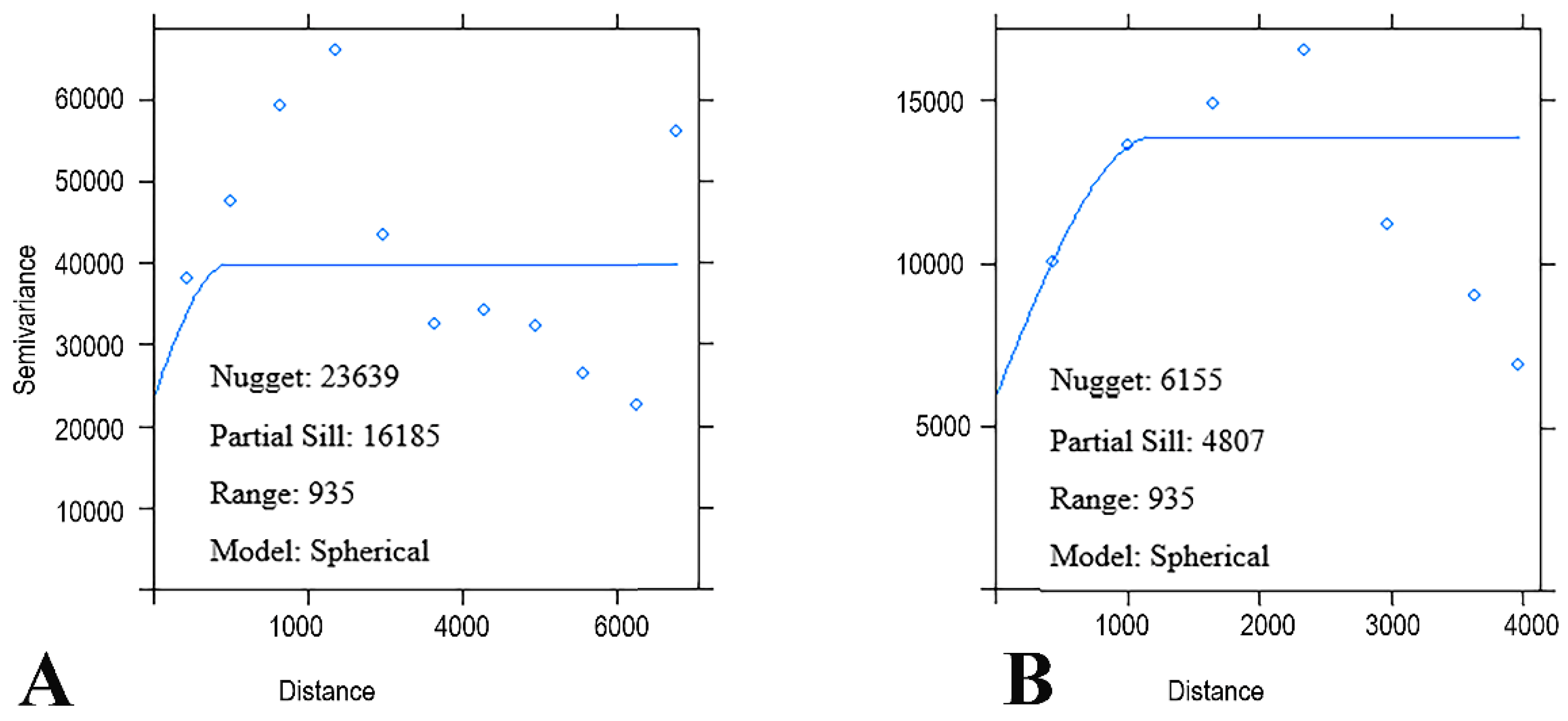
3.2. Spatial Prediction of Model Residuals

The model residuals of the two models were investigated with a multidirectional variogram. The nugget/sill ratio (N:S), which expresses the degree of spatial autocorrelation, is calculated as 59.35% and 56.14% for SVR and RF, respectively (Figure 2). The sill is the nugget plus the partial sill. Cambardella et al. [87] reported that if the N:S (nugget/sill ratio) is less than or equal to 25%, it will decisively mean strongly (S) dependent, moderately (M) spatially dependent between 25% and 75%, and >75%, weakly (W) dependent. However, it should be noted that these suggested thresholds are arbitrary, as there are no statistically defined N:S classes [36]. In our study, it is seen that the model residuals show moderate and weak spatial relationships in the two algorithms. In contrast to our values, Yang et al. [36] calculated the N:S ratio of the model residuals of the MLR as 25.98% in the Heihe river basin in north-western China. This difference is associated with the performance of different factors in estimating the environmental variable set that they used in their studies. We have produced a map of the residuals of two models using ordinary spatial kriging as a somewhat naive estimator, which provides a geostatistical foundation [35,78].

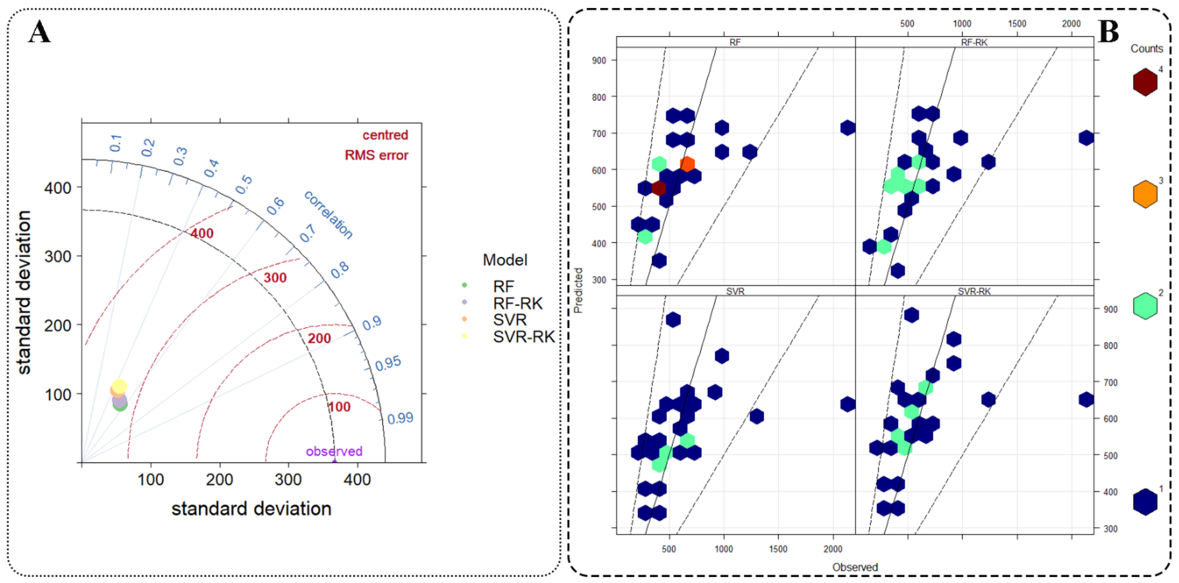
3.3. Performance of Regression-Based Algorithms and Hybrid Methods

Two algorithms evaluated the model prediction accuracy in training and validation sets on surface samples. In addition, validation was performed only on the validation dataset for the hybrid technique (Table 3 and Figure 3) [88].
As for the results, the LCCC values, which assess the agreement between the predicted and the actual values, were between 0.54 and 0.87 in the training set, while this situation changed to between 0.18 and 0.28 in the validation set (Table 3). The highest LCCC value in the training and validation sets was obtained with the RF algorithm (Table 3).
The accuracy of the modelling predictions for the validation and hybrid model validation sets was further analyzed via the Taylor diagram [89]. The Taylor diagram was used as a distinguishing tool to analyze the performance of the RF and SVR models to estimate soil EC in the validation and hybrid model validation datasets. In addition to Table 3, we report the soil salinity distribution plots measured versus the calculated soil salinity for the validation and hybrid model validation dataset with different models in Figure 3.
Literature comparisons were made according to NRMSE values because the EC value can be measured in different units, and conversions are made. Indeed, the NRMSE is related to the distributions of the training and validation sets. Taghadosi et al. [90] discussed the results of the MLR and SVR models in their study in which they used the indices calculated from Landsat 8 OLI and Sentinel 2 data as environmental variables. They received 52% NRMSE values for the training set in MLR and 44% NRMSE values for the validation set. They also found NRMSE values of 36% for the training set and 4% for the validation set using the radial basis kernel function (RBF) of SVR. Although the absence of descriptive statistics of the training and validation sets in their studies restricts the comparison with our results, lower NRMSE values compared to our study results may be attributed to the fact that they may have worked in a more homogeneous field. This inference was made from the map showing the distribution of soil samples as reported in Figure 2 in [90]. The hybrid approach, which considers the models’ residuals, slightly improved our model results. It was well known that the spatial autocorrelation degrees of the model residuals of the samples in the randomly divided training set before modelling were low [35]. Boudibi et al. [10], in their study using support vector machines (SVM) to estimate topsoil salinity in the El Outaya plain located in the northeast of Algeria, used environmental covariates including physical properties of soil, geochemical properties of groundwater, a digital elevation model, and remote sensing derivatives. They also evaluated different environmental variable combinations, and NRMSE values (SD was considered) varied between 57% and 82% for the training set and between 37% and 76% for the validation set. Considering that the coefficient of variation of EC values in their study areas is over 100% [10], our results show similarity. The reason for the NRMSE increases in our validation set in all algorithms in our study is related to the fact that the coefficient of variation is 50% higher in the validation set than in the training set. Indeed, Boudibi et al. [10] had lower CV and NRMSE values in their validation sets. Wang et al. [68] compared the 12 algorithms found in SVR and RF in their study in which they estimated the soil EC value using climate (land-surface temperature) variables, remote sensing derivatives, DEM derivatives, and landforms as environmental variables in the north-western part of the Tarim Basin in southern Xinjiang, China. In their study, NRMSE values (SD was considered) were 52% and 60% for SVR, and 49% and 56% for RF, in the training and validation set, respectively. Although these are highly similar to our results, the lower NRMSE values can be attributed to the use of their studies, a larger number of representative environmental variables, and the size of the dataset. Naimi et al. [31] investigated the effectiveness of five unique machine learning models, including the RF model, in soil salinity estimation. They reported that the NRMSE value of 34.11% (average, approximately 22% if SD was considered) produced the most successful predictions. The efficiency of cross-validation and data-splitting methods can also partially differ [28]. For sparse datasets, data splitting can be ineffective as the information in the dataset is not fully utilized for both calibration and validation. Since it is not clear how to divide the dataset, different methods are compared to confirm map accuracy [91].

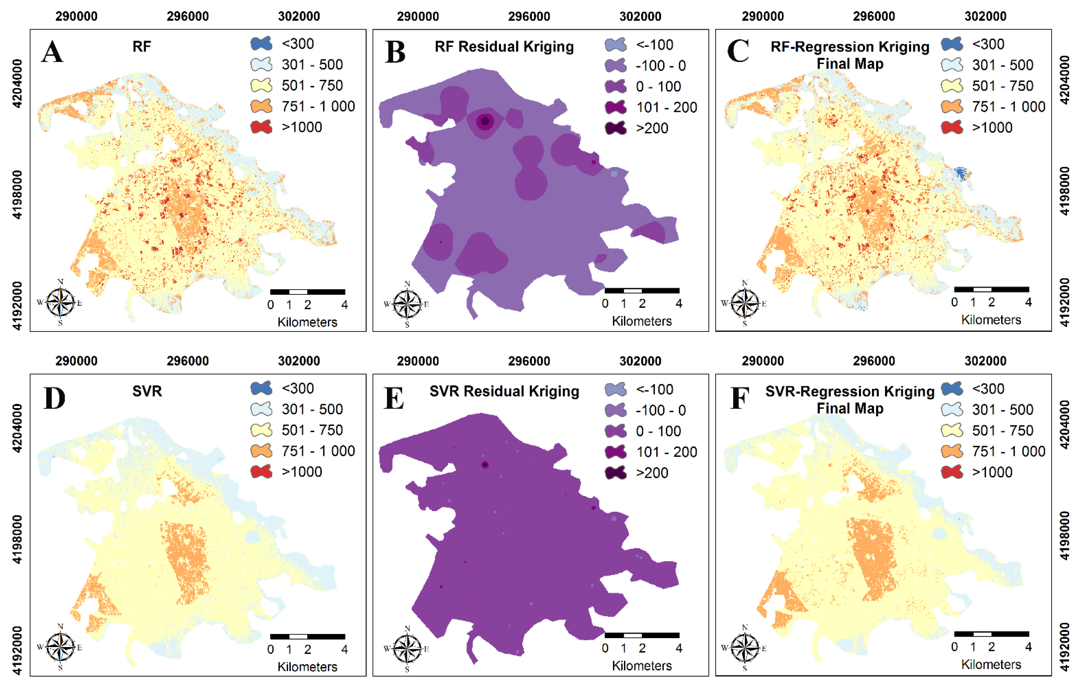
3.4. Spatial Patterns of Soil EC Dynamics

The performance of regression models derived from the machine learning algorithm was analyzed separately for SVR and RF in this study to determine the spatial distribution of soil EC.

3.4.1. Random Forest

Machine learning techniques such as RF, which can also reveal non-linear relationships, have been widely used in soil salinity mapping [31,68]. It has produced the most accurate model results and the most meaningful output soil salinity maps among the algorithms. These accuracy levels are due to the algorithm’s ability to display non-linear relationships between land observations and environmental variables. The prediction maps produced by the RF algorithm show the contribution of DEM (Figure 1b) and land cover variables to the modelling process. Low EC values are primarily distributed in the eastern parts of the current study area, where the elevation and slope are relatively high (Figure 4a). These areas have high slopes and are used as natural pastures. High EC values in depression areas of the alluvial plain were located in the irrigated agriculture areas that have been prominent for many years. Some salt discharge is likely added from the northern and eastern regions to the upper parts of the low-altitude land because of geomorphological characteristics, which result in the salt accumulation on the upper lands of the study area that have high slopes and a coarse soil texture [45], and low salt absorbability. Naimi et al. [31] reported that regions with low EC values were located at higher elevations with steeper slopes and alluvial ranges when mapping soil salinity in the Afzar region of southern Iran using the RF model. The minimum and maximum values of the EC values of the training dataset were 110 and 1692 µS cm−1, respectively (Table 2). The RF-RK hybrid method predicted the area’s minimum and maximum EC values as 172 and 1511 µS cm−1, respectively. In addition, the moderate spatial autocorrelation of the RF model residuals (Figure 4b) contributed to a better representation of the minimum and maximum value ranges in the final map. In this case, it was found to be significant when considered in terms of uncertainty assessment. The RF algorithm predicted the low EC values appropriately. However, this algorithm relatively underestimated the high EC values found in small numbers in the dataset (Figure 4c). Based on the inference information, it determined that the map produced as a result of the model created by the RF algorithm and the final map created as a result of the summing of the kriging of the model residuals could predict the areas with high salinization risk more accurately. However, it should not be forgotten that this accuracy cannot be achieved in other case studies due to the different effects of soil formation processes in different areas. For this reason, we want to draw attention to including RF algorithms in the comparative results of linear and non-linear algorithms in case studies.

3.4.2. Support Vector Regression

Support vector regression is increasingly used in spatial estimation studies of soil salinity with its different kernel functions [90,92]. The map produced by applying the SVR model to the environmental variable set in our study area was partially similar to the RF algorithm (Figure 4a,d). However, it draws back behind RF in representing the minimum and maximum values. Again, categorical environmental variables affected the SVR algorithm more (Figure 4d). Taghadosi et al. [90] reported that the most helpful soil salinity estimation maps were produced in the study areas due to using the RBF kernel function in the SVR technique. The weak spatial autocorrelation of the model residuals of the SVR did not contribute to the improvement in the final map (Figure 4f). The SVR’s map categorized distinctive areas with low salinity, high slopes, and elevation (Figure 4d,f). This research focused on comparing the performance of non-linear algorithms and how to improve the model accuracy and spatial maps of land cover classes based on long-year observation. We investigated in depth whether the model’s accuracy could describe the spatial variation in soil properties by environmental variables. Not affected or little affected soils from salinity were primarily observed in the eastern and north-eastern regions of the study area. These areas have microclimatic conditions (i.e., owing to the elevation of higher precipitation), indicating more leaching and less salt accumulation in the soil surfaces (Figure 4a,d). High soil salinity was observed around the land cover classes where permanently irrigated. Previously, especially in studies using RS indices, it was estimated that areas with bare salt cover in lakes where salinity occurs naturally contain high salt. In contrast, areas with agricultural activity with vegetation were directly defined as salt-free or slightly salty [23]. Soil salinity predictions are based on determining spectral signatures from bare surfaces or surfaces with crystals formed in remote sensing images. In this case, it is not expected that the NDVI value can indirectly determine the salinity level with soil samples taken when the annual NDVI is below the average, such as in our study area. However, our study generally found high EC values in the yearly cereal crops and perennial vegetation lands that were irrigated for many years with different irrigation methods. In such a case, the low efficiency of remote sensing data may be increased by the CLCC map. Habibi et al. [93] reported that plants such as alfalfa and cucurbits are grown in regions where the soil salinity maps produced by different machine learning algorithms are below 2000 µS cm−1 in their study comparing the distribution of salinity maps under different land uses in the Saveh plain north of Iran. In our field of study, it is necessary to develop product strategies in farming, considering the current and future water resources in the projection for the future. Considering the current spatial distribution of salinity around permanent irrigated land cover classes, it is presumed that it will cause alternative crop change in the future.

3.5. Importance of Environmental Covariates for Different Machine Learning Algorithms

The measured importance of the investigated prediction variables in the modelling process of two different machine learning algorithms is presented in Supplementary Material Figure S6. Overall, the CORINE land cover class, RS-based indices, and DEM played an essential role in developing the semi-arid region’s salinity distribution map of the alluvial plain (Supplementary Material Figure S6). Previous studies have reported that vegetation and associated covariates significantly affect soil salinity, making it an indispensable guide variable [94]. The most crucial variable in the %IncMSE significance indicator of the RF algorithm was always determined to be the permanently irrigated land (Supplementary Material Figure S6a). Aspect, NDVI, and elevation were at the forefront of ranking the most critical variables (Supplementary Material Figure S6a). In the %IncNodePurity value, which considers the squares of the residuals measuring the node impurity, the NDVI and elevation variables were maximum values. It is expected that the highest NDVI values were taken from the parcels with permanently irrigated lands in the study area. Lands of orchards, corn, sugar beet, or alfalfa may have higher NDVI values than bare soil in that period (October–November) (Supplementary Material Figure S7).
Such a case may cause significant environmental variables along with land cover classes. When receiving the satellite image, the plants mentioned above are usually in the permanent crop cover class areas. Except for the coniferous forest northwest of the study area, the plants mentioned earlier may be present in the parcels with high NDVI values (Supplementary Material Figure S6). Although we studied on a flat alluvial plain, our results expressly indicated that topographic features contribute to explaining the variability of surface soil salinity (Supplementary Material Figure S6). The increasing accessibility and quality of remote sensing products with multispectral features [95] with advancing technological advances shows promise for soil salinity estimation. However, topographic variables need to be included in the modelling process. Considering the %IncMSE value, which considers the changes in the mean square errors of the permutation-based variables in OOB, it is seen that the land cover classes representing the land use are the most critical variable. It should be emphasized that the effect of land use on salinization forecasting in agricultural areas may be more substantial than the controls of climate and topography on salinity at short distances [84]. Organic or inorganic fertilization, irrigation strategies, and crop rotation affect mineral input into the soil and surface deposition of EC in the local soil environment, resulting in significant differences in EC between different land use types. Considering the variables necessary for the support vector regression model, elevation and slope were determined (Supplementary Material Figure S6c). The CLCC categorical variables (Supplementary Material Figure S5) with codes 231, pastures, and 243, which have the lowest EC values, were higher (Supplementary Material Figure S6c). Taghizadeh-Mehrjardi et al. [94] and Abdullah et al. [96] described that covariates such as slope and NDVI are essential for soil surface salinity mapping. Since it is scarce in the literature, our study provides pioneering information demonstrating the effectiveness of land cover classes. Considering the importance levels in modelling, it can be expressed that RS-based indexes can create noise in areas with mixed land uses, and a more generalizing structure of land cover classes can improve salinity estimates using non-linear modelling algorithms.

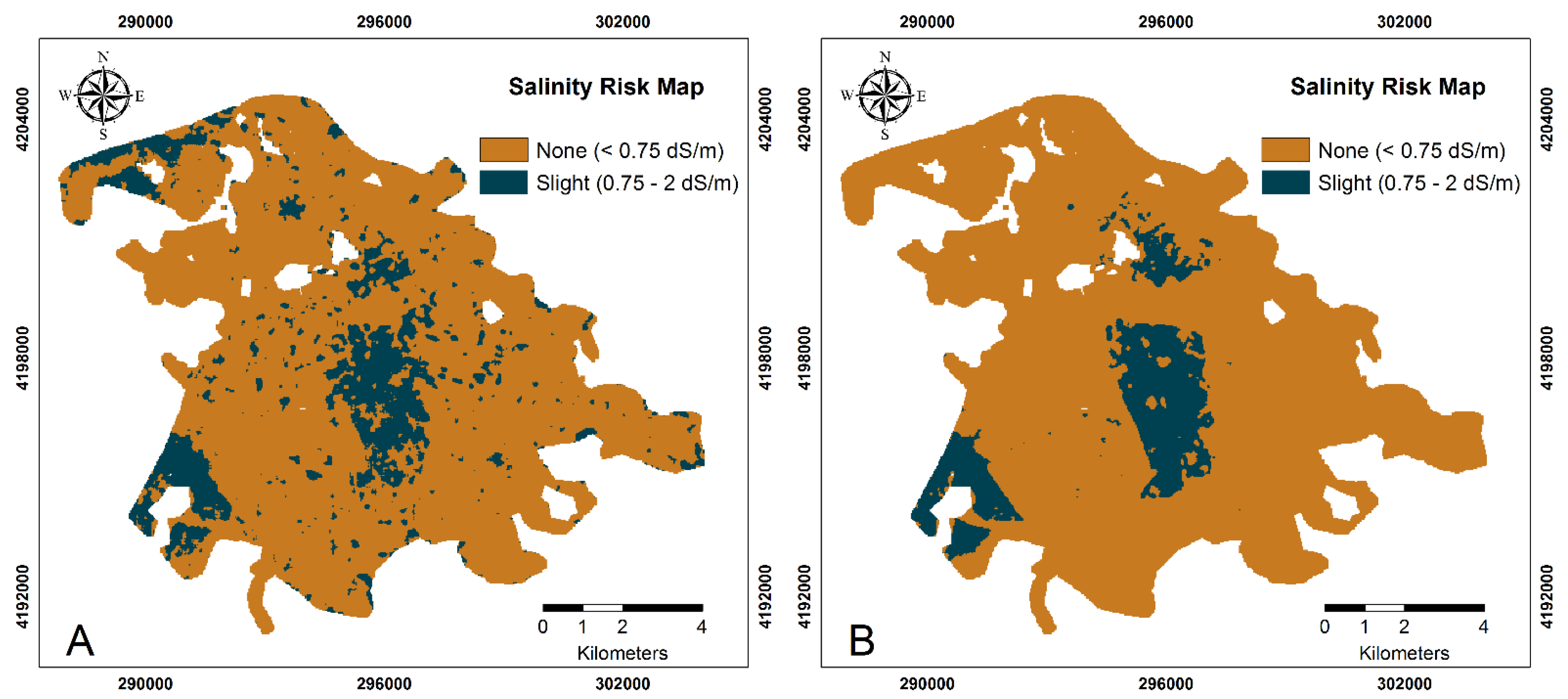
3.6. Salinity Risk Assessment

Strategic sustainable agriculture can be found in the current study area because the ground is generally almost flat, and different water resources and different irrigation methods are used effectively. Tillage agriculture is suitable in our study area, and no severe salinization problem has been detected yet. However, future concerns may arise in land cover classes where irrigated farming activities have been carried out for many years. This situation constitutes the primary motivation source of our work. Information sharing is essential for detecting or monitoring the development of salt-affected soils. Soils where salinity development is present can be determined using a parameter such as soil EC [3]. Risk maps showing the status of salinity problems in the area mapped in our current study area can be helpful for spatial information (Figure 5). The classification of the soil EC maps was produced as a result of the estimation capabilities of different algorithms with GIS tools; small risk areas were defined in various sized areas in the study area. Areas at risk of “slight” salinity were determined by the SVR in a minor area, while the highest by the RF (Figure 5 and Supplementary Material Figure S8). As a result of estimating the EC using the RF algorithm, the high EC values of the “Coniferous Forest” land cover class in the northeast of the current study area caused it to be classified as “slight” on the risk map. This is due to the RF algorithm associating the EC values with the NDVI values. This area is not an expected “slight” risk situation in the natural environment. The common aspect of the risk maps generated as a result of the two models is the determination of the “slight” salinization status in the permanently irrigated areas.

3.7. Challenges of the Case-Based Studies and Outlook Perspectives for Salinity Status Detection

Previously, researchers, for instance, Aksoy et al. [23], reported that mapping topsoil EC via multispectral satellite data could be applicable. However, the heterogeneity of the study area can significantly limit or increase the effectiveness of remote sensing data. If a salinity estimation study is carried out on the edge of a saline lake, in areas where the lake becomes smaller and land increases over time due to the decrease in precipitation and the ever-increasing evaporation rate, direct remote sensing methods through the reflection of salt crystals on the surface can be used effectively. Therefore, using a multidate series of multispectral satellite data is recommended to better represent spatial heterogeneity in areas such as our study area, where various agricultural activities have been carried out for many years [97]. In our study, the leading issue is investigating the effectiveness of land cover data for many years. In the current study area, where irrigated farming activities have been available for many years, different socio-cultural effects have shaped the land cover. Land cover classes have been prioritized to reflect these socio-cultural effects. In this regard, using single-date satellite data close to the soil sampling date constitutes one of the study’s main limitations.
We report that it does not make much sense to find out whether there is a spatial autocorrelation among the model residuals and to add these residuals with hybrid modelling techniques in the absence of spatial autocorrelation.
To comprehend the process of land deterioration and formulate efficient remediation strategies in light of the unpredictability of the future climate, it is of utmost importance to know the probability of the occurrence of salt-affected soils on the scale of the spatio-temporal distribution [14]. Therefore, determining soil EC values is progressively significant for studies to obviate soil salinization [15]. Proven methods are needed to map the spatial variability of soil EC and to manage the processes that drive soil salt transport into the root zone.
The risk of soil salinization caused by decreased water quality and increased soil salt concentrations is one of the greatest dangers to the long-term viability of agriculture that relies on irrigation. This risk ultimately results in lower crop yields and the initiation of processes that result in soil degradation. One of the most significant land-disturbing threats to harm soil fertility, stability, and biodiversity is soil salinization [14]. In the agricultural areas of the Mediterranean region, especially with summer warming being 40% faster than the global average [13], there is a higher risk of salinization in conditions of inadequate water management due to climate change. This form of soil deterioration in the Mediterranean region may become widespread in the next years. The long-term use of unsuitable irrigated agriculture, which is essential for food security (SDG 2) and adequate drinking water (SDG 6), is threatened by salinization. Due to climate change, salinization may enhance a higher problem in Mediterranean regions [98].
The spatial distribution of the salinity process of soils relies not only on factors such as land topography and climate but also on land use, which includes the human factor. Our current study reveals the effectiveness of land use by considering the long-term records of land cover in modelling. A suggestion for outlook-dedicated works on salinity is that studies should be performed to compare the potency of global land use/land cover data [25] as an open source in predicting salinity development [96].
Spatial pixel size of public or commercial satellite images has significantly progressed in the current century [95]. Thus, the commercial PlanetScope [99] is advised to use satellites, which can extend open access to spatial and radiometrically higher resolution scientific studies that can better exhibit the heterogeneous situation of salinity in agricultural areas [100].
To achieve the sustainability of agricultural systems with intensive irrigated farming activities dominant in the Mediterranean biogeography, it is necessary to determine the current situation of soil salinity in the best way possible. To this end, it is also necessary to understand the complex relationship between salinity parameters, including salinity chemistry (Cl, SO42−, HCO3, and Na+, Ca2+, Mg2+), and to identify the relevant chemical and mineralogical processes operating in soil water systems [67,86].
EC may change over time. Our research focuses on increased EC values due to irrigation, causing salinity areas to form. For this reason, more than one measurement and systematic modelling study will be the most appropriate methodology for future studies.

4. Conclusions

This current study examined the spatial assessment of the current soil EC using machine learning models in a semi-arid region of Türkiye, and environmental variables based on long-year observation in an alluvial plain irrigated for half a century. The SVR produced the most valuable and accurate maps by demonstrating the effectiveness of the LCC variable. In the current study area, LCC showed higher efficiency in modelling processes than RS and topographic features indicating the effect of long-term human activities. Although the satellite image was obtained from the barest period of the soil surface, a low correlation was found between the soil surface reflection and the EC value. The salt accumulation has not reached a level to affect the reflectance of soil surface morphology. Therefore, our results showed that land cover classes had a more substantial influence than other environmental variables in modelling anthropogenic soil salinity. We were recommended to combine land cover classes, RS data, and topographic features to reflect long-year field observations. The generated methodology would be helpful on the scale of reconnaissance studies to identify hot spots that may develop a salinity hazard because these data types are open-source and can be used for soil salinity in future projections. As a result of the study, it is possible to foresee the integration of topographic features, land cover classes, and RS data can be used successfully in the projection of other dynamic soil properties in arable land. Using this approach, information can be primarily generalized, thereby reducing the time and cost spent on obtaining the result of laboratory analysis. This approach is an important stage for the prediction of soil properties of land with no soil information and that is small-scale fragmented.
LCC-based salinization forecasting can give policymakers a chance to plan ahead to counteract the risks of climate change. As a temporal variable, CORINE may offer a chance to take this approach.

Supplementary Materials

The following supporting information can be downloaded at: www.mdpi.com/article/10.3390/land11122148/s1, Figure S1: The study area climograph (above) and model report (below) produced using jNSM v1.6.0; Figure S2: CORINE datasets for many years of study area (A:1990, B:2000; C:2006; D:2012); Figure S3: Flowchart of the methodology; Figure S4: Density graph of the EC values of the samples in the training and validation set; Figure S5. Comparison of EC values of soil samples according to land cover classes; Figure S6: Variable importance for each algorithm. A: random forest—%IncMSE; B: random forest—%IncNodePurity, C: support vector regression. Figure S7: NDVI variable map used in the study. Figure S8. Salinity risk levels (a) percent of area, (b) field size. RF: Random forest, SVR: support vector regression. Table S1: Spearman correlation coefficients among the EC and some physical and chemical soil properties for all soil samples.

Author Contributions

Conceptualization, F.K. and L.B.; methodology, F.K. and L.B.; software, F.K.; formal analysis, F.K.; investigation, F.K. resources, F.K.; data curation, F.K. and C.S.; writing—original draft preparation, F.K. and C.S; writing—review and editing, F.K., C.S., L.B. and A.K.; visualization, F.K. and C.S; supervision, L.B. All authors have read and agreed to the published version of the manuscript.

Funding

This research received no external funding.

Institutional Review Board Statement

Not applicable.

Informed Consent Statement

Not applicable.

Data Availability Statement

Data available on request due to restrictions.

Acknowledgments

The first phase of this study was the abstract presented at the virtual Global Symposium on Salt-affected Soils (GSAS21); “Spatial predictability of salinity hazard with machine learning algorithms and digital data in the Irrigation Plain”, THEME 1: Assessment, mapping, and monitoring of salt-affected soils, online, 20–22 October 2021. We would like to thank the participants who contributed with their valuable comments in Day 2 Parallel session 1. Fuat KAYA is member of SAS & Assessment working group of INSAS (INTERNATIONAL NETWORK ON SALT-AFFECTED SOILS). All authors have read and agreed to the acknowledgement section.

Conflicts of Interest

The authors declare no conflict of interest.

References

  1. Ivushkin, K.; Bartholomeus, H.; Bregt, A.K.; Pulatov, A.; Kempen, B.; de Sousa, L. Global Mapping of Soil Salinity Change. Remote Sens. Environ. 2019, 231, 111260. [Google Scholar] [CrossRef]
  2. Bouma, J.; Bonfante, A.; Basile, A.; van Tol, J.; Hack-ten Broeke, M.J.D.; Mulder, M.; Heinen, M.; Rossiter, D.G.; Poggio, L.; Hirmas, D.R. How Can Pedology and Soil Classification Contribute towards Sustainable Development as a Data Source and Information Carrier? Geoderma 2022, 424, 115988. [Google Scholar] [CrossRef]
  3. Omuto, C.T.; Vargas, R.R.; el Mobarak, A.M.; Mohamed, N.; Viatkin, K.; Yigini, Y. Mapping of Salt-Affected Soils: Technical Manual, 1st ed.; FAO: Rome, Italy, 2020. [Google Scholar]
  4. Omuto, C.T.; Vargas, R.R.; Elmobarak, A.A.; Mapeshoane, B.E.; Koetlisi, K.A.; Ahmadzai, H.; Abdalla Mohamed, N. Digital Soil Assessment in Support of a Soil Information System for Monitoring Salinization and Sodification in Agricultural Areas. Land Degrad. Dev. 2022, 33, 1204–1218. [Google Scholar] [CrossRef]
  5. Hopmans, J.W.; Qureshi, A.S.; Kisekka, I.; Munns, R.; Grattan, S.R.; Rengasamy, P.; Ben-Gal, A.; Assouline, S.; Javaux, M.; Minhas, P.S.; et al. Critical Knowledge Gaps and Research Priorities in Global Soil Salinity. Adv. Agron. 2021, 169, 1–191. [Google Scholar] [CrossRef]
  6. Ghiglieri, G.; Carletti, A.; Pittalis, D. Analysis of Salinization Processes in the Coastal Carbonate Aquifer of Porto Torres (NW Sardinia, Italy). J. Hydrol. 2012, 432–433, 43–51. [Google Scholar] [CrossRef]
  7. Konyushkova, M.; Alavipanah, S.; Heidari, A.; Kozlov, D.; Yu, M.; Semenkov, I. Spatial and Seasonal Salt Translocation in the Young Soils at the Coastal Plains of the Caspian Sea. Quat. Int. 2021, 590, 15–25. [Google Scholar] [CrossRef]
  8. FAO-ITPS Salt-Affected Soils Are a Global Issue. Available online: https://www.fao.org/3/cb4809en/cb4809en.pdf (accessed on 7 September 2022).
  9. Manuel, R.; Machado, A.; Serralheiro, R.P.; Alvino, A.; Freire, M.I.; Ferreira, R. Soil Salinity: Effect on Vegetable Crop Growth. Management Practices to Prevent and Mitigate Soil Salinization. Horticulturae 2017, 3, 30. [Google Scholar] [CrossRef] [Green Version]
  10. Boudibi, S.; Sakaa, B.; Benguega, Z.; Fadlaoui, H.; Othman, T.; Bouzidi, N. Spatial Prediction and Modeling of Soil Salinity Using Simple Cokriging, Artificial Neural Networks, and Support Vector Machines in El Outaya Plain, Biskra, Southeastern Algeria. Acta Geochim. 2021, 40, 390–408. [Google Scholar] [CrossRef]
  11. Iglesias, A.; Quiroga, S.; Moneo, M.; Garrote, L. From Climate Change Impacts to the Development of Adaptation Strategies: Challenges for Agriculture in Europe. Clim. Chang. 2012, 112, 143–168. [Google Scholar] [CrossRef]
  12. Haddeland, I.; Heinke, J.; Biemans, H.; Eisner, S.; Flörke, M.; Hanasaki, N.; Konzmann, M.; Ludwig, F.; Masaki, Y.; Schewe, J.; et al. Global Water Resources Affected by Human Interventions and Climate Change. Proc. Natl. Acad. Sci. USA 2014, 111, 3251–3256. [Google Scholar] [CrossRef]
  13. Cramer, W.; Guiot, J.; Fader, M.; Garrabou, J.; Gattuso, J.P.; Iglesias, A.; Lange, M.A.; Lionello, P.; Llasat, M.C.; Paz, S.; et al. Climate Change and Interconnected Risks to Sustainable Development in the Mediterranean. Nat. Clim. Chang. 2018, 8, 972–980. [Google Scholar] [CrossRef] [Green Version]
  14. Hassani, A.; Azapagic, A.; Shokri, N. Predicting Long-Term Dynamics of Soil Salinity and Sodicity on a Global Scale. Proc. Natl. Acad. Sci. USA 2020, 117, 33017–33027. [Google Scholar] [CrossRef] [PubMed]
  15. Okur, B.; Örçen, N. Soil Salinization and Climate Change. In Climate Change and Soil Interactions; Elsevier: New York, NY, USA, 2020; pp. 331–350. [Google Scholar] [CrossRef]
  16. Kendirli, B.; Cakmak, B.; Ucar, Y. Salinity in the Southeastern Anatolia Project (GAP), Turkey: Issues and Options. Irrig. Drain. 2005, 54, 115–122. [Google Scholar] [CrossRef]
  17. Çullu, M.A.; Aydemir, S.; Qadir, M.; Almaca, A.; Öztürkmen, A.R.; Bilgiç, A.; Aǧca, N. Implication of Groundwater Fluctuation on the Seasonal Salt Dynamic in the Harran Plain, South-Eastern Turkey. Irrig. Drain. 2010, 59, 465–476. [Google Scholar] [CrossRef]
  18. Bilgili, A.V. Spatial Assessment of Soil Salinity in the Harran Plain Using Multiple Kriging Techniques. Environ. Monit Assess 2013, 185, 777–795. [Google Scholar] [CrossRef] [PubMed]
  19. FAO GSASmap v1.0, Global Map of Salt-Affected Soils. Available online: https://www.fao.org/3/cb7247en/cb7247en.pdf (accessed on 7 September 2022).
  20. McBratney, A.B.; Mendonça Santos, M.L.; Minasny, B. On Digital Soil Mapping. Geoderma 2003, 117, 3–52. [Google Scholar] [CrossRef]
  21. Mponela, P.; Snapp, S.; Villamor, G.B.; Tamene, L.; Le, Q.B.; Borgemeister, C. Digital Soil Mapping of Nitrogen, Phosphorus, Potassium, Organic Carbon and Their Crop Response Thresholds in Smallholder Managed Escarpments of Malawi. Appl. Geogr. 2020, 124, 102299. [Google Scholar] [CrossRef]
  22. Bakacsi, Z.; Tóth, T.; Makó, A.; Barna, G.; Laborczi, A.; Szabó, J.; Szatmári, G.; Pásztor, L. National Level Assessment of Soil Salinization and Structural Degradation Risks under Irrigation. Hung. Geogr. Bull. 2019, 68, 141–156. [Google Scholar] [CrossRef]
  23. Aksoy, S.; Yildirim, A.; Gorji, T.; Hamzehpour, N.; Tanik, A.; Sertel, E. Assessing the Performance of Machine Learning Algorithms for Soil Salinity Mapping in Google Earth Engine Platform Using Sentinel-2A and Landsat-8 OLI Data. Adv. Space Res. 2022, 69, 1072–1086. [Google Scholar] [CrossRef]
  24. Bannari, A.; Abuelgasim, A. Potential and Limits of Vegetation Indices Compared to Evaporite Mineral Indices for Soil Salinity Discrimination and Mapping. SOIL Discuss. 2021, 1–48. [Google Scholar] [CrossRef]
  25. Karra, K.; Kontgis, C.; Statman-Weil, Z.; Mazzariello, J.C.; Mathis, M.; Brumby, S.P. Global Land Use/Land Cover with Sentinel 2 and Deep Learning. In Proceedings of the 2021 IEEE International Geoscience and Remote Sensing Symposium IGARSS, Brussels, Belgium, 11–16 July 2021; pp. 4704–4707. [Google Scholar] [CrossRef]
  26. Zhang, T.T.; Zeng, S.L.; Gao, Y.; Ouyang, Z.T.; Li, B.; Fang, C.M.; Zhao, B. Assessing Impact of Land Uses on Land Salinization in the Yellow River Delta, China Using an Integrated and Spatial Statistical Model. Land Use Policy 2011, 28, 857–866. [Google Scholar] [CrossRef]
  27. Poggio, L.; de Sousa, L.; Genova, G.; D’Angelo, P.; Schwind, P.; Heiden, U. Soil organic carbon modelling with digital soil mapping and remote sensing for permanently vegetated areas. In Proceedings of the 2021 IEEE International Geoscience and Remote Sensing Symposium IGARSS, Brussels, Belgium, 11–16 July 2021; pp. 492–494. [Google Scholar] [CrossRef]
  28. FAO Soil Organic Carbon Mapping Cookbook. Available online: https://www.fao.org/documents/card/en/c/I8895EN/ (accessed on 7 September 2022).
  29. Davis, E.; Wang, C.; Dow, K. Comparing Sentinel-2 MSI and Landsat 8 OLI in Soil Salinity Detection: A Case Study of Agricultural Lands in Coastal North Carolina. Int. J. Remote Sens. 2019, 40, 6134–6153. [Google Scholar] [CrossRef]
  30. Maleki, S.; Fathizad, H.; Karimi, A.; Taghizadeh-Mehrjardi, R.; Pourghasemi, H.R. Monitoring of Spatiotemporal Changes of Soil Salinity and Alkalinity in Eastern and Central Parts of Iran. In Computers in Earth and Environmental Sciences; Elsevier: New York, NY, USA, 2022; pp. 547–561. [Google Scholar]
  31. Naimi, S.; Ayoubi, S.; Zeraatpisheh, M.; Dematte, J.A.M. Ground Observations and Environmental Covariates Integration for Mapping of Soil Salinity: A Machine Learning-Based Approach. Remote Sens. 2021, 13, 4825. [Google Scholar] [CrossRef]
  32. Zhao, D.; Arshad, M.; Wang, J.; Triantafilis, J. Soil Exchangeable Cations Estimation Using Vis-NIR Spectroscopy in Different Depths: Effects of Multiple Calibration Models and Spiking. Comput. Electron. Agric. 2021, 182, 105990. [Google Scholar] [CrossRef]
  33. Zhao, D.; Li, N.; Zare, E.; Wang, J.; Triantafilis, J. Mapping Cation Exchange Capacity Using a Quasi-3d Joint Inversion of EM38 and EM31 Data. Soil Tillage Res. 2020, 200, 104618. [Google Scholar] [CrossRef]
  34. Zhao, D.; Zhao, X.; Khongnawang, T.; Arshad, M.; Triantafilis, J. A Vis-NIR Spectral Library to Predict Clay in Australian Cotton Growing Soil. Soil Sci. Soc. Am. J. 2018, 82, 1347–1357. [Google Scholar] [CrossRef]
  35. Hengl, T.; Nussbaum, M.; Wright, M.N.; Heuvelink, G.B.M.; Gräler, B. Random Forest as a Generic Framework for Predictive Modeling of Spatial and Spatio-Temporal Variables. PeerJ 2018, 2018, e5518. [Google Scholar] [CrossRef]
  36. Yang, S.H.; Liu, F.; Song, X.D.; Lu, Y.Y.; Li, D.C.; Zhao, Y.G.; Zhang, G.L. Mapping Topsoil Electrical Conductivity by a Mixed Geographically Weighted Regression Kriging: A Case Study in the Heihe River Basin, Northwest China. Ecol. Indic. 2019, 102, 252–264. [Google Scholar] [CrossRef]
  37. Wadoux, A.M.J.C.; Román-Dobarco, M.; McBratney, A.B. Perspectives on Data-Driven Soil Research. Eur. J. Soil Sci. 2021, 72, 1675–1689. [Google Scholar] [CrossRef]
  38. Kaya, F.; Başayiğit, L. Using Machine Learning Algorithms to Mapping of the Soil Macronutrient Elements Variability with Digital Environmental Data in an Alluvial Plain. In Artificial Intelligence and Smart Agriculture Applications; Kose, U., Prasath, V.B.S., Mondal, M.R.H., Podder, P., Subrato, B., Eds.; Auerbach Publications: Boca Raton, FL, USA, 2022; pp. 107–136. [Google Scholar]
  39. Kaya, F.; Başayiğit, L.; Keshavarzi, A.; Francaviglia, R. Digital Mapping for Soil Texture Class Prediction in Northwestern Türkiye by Different Machine Learning Algorithms. Geoderma Reg. 2022, 31, e00584. [Google Scholar] [CrossRef]
  40. van Wambeke, A.R. JNSM—Java Newhall Simulation Model JNSM—The Newhall Simulation Model for Estimating Soil Moisture & Temperature Regimes; USDA: Indianapolis, IN, USA, 2000; pp. 1–9.
  41. GDSHW. Isparta Atabey Plain Irrigation Rehabilitation Project Resettlement Action Plan. 2020. Available online: https://jagomart.net/item/25154/isparta-atabey-plain-irrigation-rehabilitation-project-first-phase-resettlement-action-plan-may-2021 (accessed on 7 September 2022).
  42. TSMS. Climate of Turkey According to Köppen Climate Classification. Available online: https://www.mgm.gov.tr/FILES/iklim/iklim_siniflandirmalari/koppen.pdf (accessed on 7 September 2022).
  43. Soil Survey Staff Keys to Soil Taxonomy, 12th ed.; USDA-Natural Resources Conservation Service: Washington, DC, USA, 2014.
  44. European Union. C.L.M.S. Corine Land Cover Class 2018 V 2.0 Data. Available online: https://land.copernicus.eu/pan-european/corine-land-cover (accessed on 7 September 2022).
  45. Kaya, F.; Başayiğit, L. Spatial Prediction and Digital Mapping of Soil Texture Classes in a Floodplain Using Multinomial Logistic Regression. In Intelligent and Fuzzy Techniques for Emerging Conditions and Digital Transformation; Kahraman, C., Cebi, S., Onar Cevik, S., Oztaysi, B., Tolga, A.C., Sari, I.U., Eds.; Springer: Berlin/Heidelberg, Germany, 2022; pp. 463–473. [Google Scholar]
  46. Soil Science Division Staff. Soil Survey Manual; Ditzler, C., Scheffe, K., Monger, H.C., Eds.; USDA Handbook 18; Government Printing Office: Washington, DC, USA, 2017.
  47. Rhoades, J.D.; Chanduvi, F.; Lesch, S. Soil Salinity Assessment: Methods and Interpretation of Electrical Conductivity Measurements. Available online: https://www.fao.org/3/x2002e/x2002e.pdf (accessed on 7 September 2022).
  48. Bouyoucos, G.J. Hydrometer Method Improved for Making Particle Size Analyses of Soils1. Agron. J. 1962, 54, 464–465. [Google Scholar] [CrossRef]
  49. EPA. Available online: https://www.epa.gov/sites/default/files/2015-12/documents/9081.pdf (accessed on 21 November 2022).
  50. Kacar, B. Fiziksel ve Kimyasal Toprak Analizler, 1st ed.; Nobel: Ankara, Turkey, 2016; ISBN 9786053204305. [Google Scholar]
  51. Schillaci, C.; Braun, A.; Kropáček, J. Terrain Analysis and Landform Recognition. In Geomorphological Techniques (Online Edition); Clarke, N.E., Nield, J.M., Eds.; British Society for Geomorphology: London, UK, 2015. [Google Scholar]
  52. Mulder, V.L.; de Bruin, S.; Schaepman, M.E.; Mayr, T.R. The Use of Remote Sensing in Soil and Terrain Mapping—A Review. Geoderma 2011, 162, 1–19. [Google Scholar] [CrossRef]
  53. Silva, B.P.C.; Silva, M.L.N.; Avalos, F.A.P.; de Menezes, M.D.; Curi, N. Digital Soil Mapping Including Additional Point Sampling in Posses Ecosystem Services Pilot Watershed, Southeastern Brazil. Sci. Rep. 2019, 9, 13763. [Google Scholar] [CrossRef] [PubMed] [Green Version]
  54. Yahiaoui, I.; Douaoui, A.; Zhang, Q.; Ziane, A. Soil Salinity Prediction in the Lower Cheliff Plain (Algeria) Based on Remote Sensing and Topographic Feature Analysis. J. Arid Land 2015, 7, 794–805. [Google Scholar] [CrossRef]
  55. Ma, G.; Ding, J.; Han, L.; Zhang, Z.; Ran, S. Digital Mapping of Soil Salinization Based on Sentinel-1 and Sentinel-2 Data Combined with Machine Learning Algorithms. Reg. Sustain. 2021, 2, 177–188. [Google Scholar] [CrossRef]
  56. ASF DAAC. ALOS PALSAR_Radiometric_Terrain_Corrected_high_res; Includes Material © JAXA/METI 2007. Available online: https://asf.alaska.edu/data-sets/derived-data-sets/alos-palsar-rtc/alos-palsar-radiometric-terrain-correction/ (accessed on 5 September 2021). [CrossRef]
  57. Gruber, S.; Peckham, S. Chapter 7 Land-Surface Parameters and Objects in Hydrology. In Developments in Soil Science; Elsevier: New York, NY, USA, 2009; Volume 33, pp. 171–194. [Google Scholar]
  58. Sentinel-2 User Handbook; 1.2; European Space Agency (ESA): Paris, France, 2015.
  59. Xiao, J.; Shen, Y.; Tateishi, R.; Bayaer, W. Development of Topsoil Grain Size Index for Monitoring Desertification in Arid Land Using Remote Sensing. Int. J. Remote Sens. 2007, 27, 2411–2422. [Google Scholar] [CrossRef]
  60. Hounkpatin, K.O.L.; Schmidt, K.; Stumpf, F.; Forkuor, G.; Behrens, T.; Scholten, T.; Amelung, W.; Welp, G. Predicting Reference Soil Groups Using Legacy Data: A Data Pruning and Random Forest Approach for Tropical Environment (Dano Catchment, Burkina Faso). Sci. Rep. 2018, 8, 9959. [Google Scholar] [CrossRef] [Green Version]
  61. Brown, K.S.; Libohova, Z.; Boettinger, J. Digital Soil Mapping. In Soil Survey Manual; Ditzler, C., Scheffe, K., Monger, H.C., Eds.; USDA Handbook 18; Government Printing Office: Washington, DC, USA, 2017. [Google Scholar]
  62. Ließ, M.; Gebauer, A.; Don, A. Machine Learning With GA Optimization to Model the Agricultural Soil-Landscape of Germany: An Approach Involving Soil Functional Types With Their Multivariate Parameter Distributions Along the Depth Profile. Front. Environ. Sci. 2021, 9, 212. [Google Scholar] [CrossRef]
  63. ESRI. ArcGIS User’s Guide. 2022. Available online: http://www.esri.com (accessed on 15 September 2022).
  64. R Core Team. R: A Language and Environment for Statistical Computing; R Foundation for Statistical Computing: Vienna, Austria, 2019; Available online: https://www.r-project.org/ (accessed on 6 July 2022).
  65. Hijmans, R.J. Raster: Geographic Data Analysis and Modeling. 2022. Available online: https://cran.r-project.org/web/packages/raster/raster.pdf (accessed on 6 July 2022).
  66. Revelle, W. Psych: Procedures for Psychological, Psychometric, and Personality Research. 2022. Available online: https://www.scholars.northwestern.edu/en/publications/psych-procedures-for-personality-and-psychological-research (accessed on 6 July 2022).
  67. Ismayilov, A.I.; Mamedov, A.I.; Fujimaki, H.; Tsunekawa, A.; Levy, G.J. Soil Salinity Type Effects on the Relationship between the Electrical Conductivity and Salt Content for 1:5 Soil-to-Water Extract. Sustainability 2021, 13, 3395. [Google Scholar] [CrossRef]
  68. Wang, F.; Shi, Z.; Biswas, A.; Yang, S.; Ding, J. Multi-Algorithm Comparison for Predicting Soil Salinity. Geoderma 2020, 365, 114211. [Google Scholar] [CrossRef]
  69. Breiman, L. Random Forests. Mach. Learn. 2001, 45, 5–32. [Google Scholar] [CrossRef] [Green Version]
  70. Liaw, A.; Wiener, M. Classification and Regression by RandomForest. R News 2002, 2, 18–22. [Google Scholar]
  71. Biau, G.; Scornet, E. A Random Forest Guided Tour. Test 2016, 25, 197–227. [Google Scholar] [CrossRef] [Green Version]
  72. Cortes, C.; Vapnik, V.; Saitta, L. Support-Vector Networks. Mach. Learn. 1995, 20, 273–297. [Google Scholar] [CrossRef]
  73. Drucker, H.; Burges, C.J.; Kaufman, L.; Smola, A.; Vapnik, V. Support Vector Regression Machines. Adv. Neural Inf. Process. Syst. 1996, 9, 155–161. [Google Scholar]
  74. Chang, C.C.; Lin, C.J. LIBSVM. ACM Trans. Intell. Syst. Technol. (TIST) 2011, 2, 27. [Google Scholar] [CrossRef]
  75. Meyer, D.; Dimitriadou, E.; Hornik, K.; Weingessel, A.; Leisch, F. E1071: Misc Functions of the Department of Statistics; Probability Group (Formerly: E1071), TU Wien: Vienna, Austria, 2022. [Google Scholar]
  76. Hengl, T.; Macmillan, R.A. Predictive Soil Mapping with R; OpenGeoHub Foundation: Wageningen, The Netherlands, 2019; pp. 227–273. [Google Scholar]
  77. Tziachris, P.; Aschonitis, V.; Chatzistathis, T.; Papadopoulou, M. Assessment of Spatial Hybrid Methods for Predicting Soil Organic Matter Using DEM Derivatives and Soil Parameters. Catena 2019, 174, 206–216. [Google Scholar] [CrossRef]
  78. Gräler, B.; Pebesma, E.; Heuvelink, G. Spatio-Temporal Interpolation Using Gstat. R J. 2016, 8, 204. [Google Scholar] [CrossRef]
  79. Keshavarzi, A.; Tuffour, H.O.; Oppong, J.C.; Zeraatpisheh, M.; Kumar, V. Dealing with Soil Organic Carbon Modeling: Some Insights from an Agro-Ecosystem in Northeast Iran. Earth Sci. Inf. 2021, 14, 1833–1845. [Google Scholar] [CrossRef]
  80. Zambrano-Bigiarini, M. HydroGOF: Goodness-of-Fit Functions for Comparison of Simulated and Observed Hydrological Time Series. 2020. Available online: https://www.rforge.net/hydroGOF/git.html (accessed on 6 July 2022).
  81. Lin, L.I.-K. A Concordance Correlation Coefficient to Evaluate Reproducibility. Biometrics 1989, 45, 255. [Google Scholar] [CrossRef] [PubMed]
  82. Wilding, L.P. Spatial Variability: Its Documentation, Accommodation, and Implication to Soil Surveys. In Soil Spatial Variability; Nielsen, D.R., Bouma, J., Eds.; Pudoc: Wageningen, The Netherlands, 1985; pp. 166–193. [Google Scholar]
  83. Fathizad, H.; Ali Hakimzadeh Ardakani, M.; Sodaiezadeh, H.; Kerry, R.; Taghizadeh-Mehrjardi, R. Investigation of the Spatial and Temporal Variation of Soil Salinity Using Random Forests in the Central Desert of Iran. Geoderma 2020, 365, 114233. [Google Scholar] [CrossRef]
  84. Nosetto, M.D.; Acosta, A.M.; Jayawickreme, D.H.; Ballesteros, S.I.; Jackson, R.B.; Jobbágy, E.G. Land-Use and Topography Shape Soil and Groundwater Salinity in Central Argentina. Agric. Water Manag. 2013, 129, 120–129. [Google Scholar] [CrossRef]
  85. Jiang, Q.; Peng, J.; Biswas, A.; Hu, J.; Zhao, R.; He, K.; Shi, Z. Characterising Dryland Salinity in Three Dimensions. Sci. Total Environ. 2019, 682, 190–199. [Google Scholar] [CrossRef]
  86. Kargas, G.; Londra, P.; Sotirakoglou, K. The Effect of Soil Texture on the Conversion Factor of 1:5 Soil/Water Extract Electrical Conductivity (EC1:5) to Soil Saturated Paste Extract Electrical Conductivity (ECe). Water 2022, 14, 642. [Google Scholar] [CrossRef]
  87. Cambardella, C.A.; Moorman, T.B.; Novak, J.M.; Parkin, T.B.; Karlen, D.L.; Turco, R.F.; Konopka, A.E. Field-Scale Variability of Soil Properties in Central Iowa Soils. Soil Sci. Soc. Am. J. 1994, 58, 1501–1511. [Google Scholar] [CrossRef]
  88. Malone, B.P.; Minasny, B.; McBratney, A.B. Continuous Soil Attribute Modeling and Mapping. In Using R for Digital Soil Mapping; Springer: Cham, Switzerland, 2017; pp. 117–149. [Google Scholar]
  89. Mishra, G.; Sulieman, M.M.; Kaya, F.; Francaviglia, R.; Keshavarzi, A.; Bakhshandeh, E.; Loum, M.; Jangir, A.; Ahmed, I.; Elmobarak, A.; et al. Machine Learning for Cation Exchange Capacity Prediction in Different Land Uses. Catena 2022, 216, 106404. [Google Scholar] [CrossRef]
  90. Taghadosi, M.M.; Hasanlou, M.; Eftekhari, K. Retrieval of Soil Salinity from Sentinel-2 Multispectral Imagery. Eur. J. Remote Sens. 2019, 52, 138–154. [Google Scholar] [CrossRef] [Green Version]
  91. Wadoux, A.M.J.C.; Heuvelink, G.B.M.; de Bruin, S.; Brus, D.J. Spatial Cross-Validation Is Not the Right Way to Evaluate Map Accuracy. Ecol. Model. 2021, 457, 109692. [Google Scholar] [CrossRef]
  92. Wang, J.; Peng, J.; Li, H.; Yin, C.; Liu, W.; Wang, T.; Zhang, H. Soil Salinity Mapping Using Machine Learning Algorithms with the Sentinel-2 MSI in Arid Areas, China. Remote Sens. 2021, 13, 305. [Google Scholar] [CrossRef]
  93. Habibi, V.; Ahmadi, H.; Jafari, M.; Moeini, A. Machine Learning and Multispectral Data-Based Detection of Soil Salinity in an Arid Region, Central Iran. Environ. Monit. Assess. 2020, 192, 759. [Google Scholar] [CrossRef] [PubMed]
  94. Taghizadeh-Mehrjardi, R.; Schmidt, K.; Toomanian, N.; Heung, B.; Behrens, T.; Mosavi, A.; Band, S.; Amirian-Chakan, A.; Fathabadi, A.; Scholten, T. Improving the Spatial Prediction of Soil Salinity in Arid Regions Using Wavelet Transformation and Support Vector Regression Models. Geoderma 2021, 383, 114793. [Google Scholar] [CrossRef]
  95. Burke, M.; Driscoll, A.; Lobell, D.B.; Ermon, S. Using Satellite Imagery to Understand and Promote Sustainable Development. Science 2021, 371, 6535. [Google Scholar] [CrossRef] [PubMed]
  96. Abdullah, A.Y.M.; Biswas, R.K.; Chowdhury, A.I.; Billah, S.M. Modeling Soil Salinity Using Direct and Indirect Measurement Techniques: A Comparative Analysis. Environ. Dev. 2019, 29, 67–80. [Google Scholar] [CrossRef]
  97. Szatmári, G.; Bakacsi, Z.; Laborczi, A.; Petrik, O.; Pataki, R.; Tóth, T.; Pásztor, L. Elaborating Hungarian Segment of the Global Map of Salt-Affected Soils (GSSmap): National Contribution to an International Initiative. Remote Sens. 2020, 12, 4073. [Google Scholar] [CrossRef]
  98. Keesstra, S.; Mol, G.; de Leeuw, J.; Okx, J.; Molenaar, C.; de Cleen, M.; Visser, S. Soil-Related Sustainable Development Goals: Four Concepts to Make Land Degradation Neutrality and Restoration Work. Land 2018, 7, 133. [Google Scholar] [CrossRef] [Green Version]
  99. Planet Team Planet Application Program Interface. Available online: https://www.planet.com/explorer/ (accessed on 8 September 2022).
  100. Avdan, U.; Kaplan, G.; Küçük Matcı, D.; Yiğit Avdan, Z.; Erdem, F.; Tuğba Mızık, E.; Demirtaş, İ. Soil Salinity Prediction Models Constructed by Different Remote Sensors. Phys. Chem. Earth Parts A/B/C 2022, 128, 103230. [Google Scholar] [CrossRef]
Figure 1. The location of the study area and the spatial distribution of the soil samples are overlaid on a CORINE 2018 land cover map (A) and DEM (B).
Land 11 02148 g001
Figure 2. Strength of the spatial autocorrelation among evaluated model residuals for EC. SVR: support vector regression (A), RF: random forest (B).
Land 11 02148 g002
Figure 3. Taylor diagram for validation and hybrid model validation dataset (A). Predicted vs. observed soil EC in validation and hybrid model validation datasets (B). Abbreviations: SVR: support vector regression, RF: random forest, RK: regression-kriging.
Land 11 02148 g003
Figure 4. Predicted soil EC map for two algorithms and hybrid techniques. (AC) Random forest predicted EC map, model residuals of RF kriging map, RF-RK final map, respectively. (DF) Support vector regression indicated EC map, model residuals of SVR kriging map, SVR-RK final map, respectively.
Land 11 02148 g004
Figure 5. Salinity risk assessment maps. A: Random forest, B: support vector regression.
Land 11 02148 g005
Table 2. Descriptive statistics of EC and some physical and chemical soil properties.
VariableDatasetMeanSDCVMinimumMaximumSkewnessKurtosis
ECTraining616.30249.6040.49110.01692.01.294.47
Validation602.80366.6060.82152.02068.02.649.14
Clay (%)All36.9113.6837.0613.2873.760.82−0.22
Sand (%)37.2915.0140.256.3569.30−0.34−0.87
Silt (%)25.817.1627.7412.4751.941.131.64
CEC (cmolc kg−1)22.756.7529.679.3440.240.710.05
SSP (%)36.765.9316.1320.5050.00−0.18−0.22
Abbreviations: EC: electrical conductivity (µS cm−1); CV: coefficient of variation (%); SD: standard deviation; CEC: cation exchange capacity; SSP: soil saturation percentage.
Table 3. Comparison of model performance criteria of different algorithms in predicting EC.
Soil PropertyModelTrainingValidationHybrid Model Validation
LCCCRMSENRMSELCCCNRMSELCCCNRMSE
ECSVR0.50198.0579.40.2589.60.2688.7
RF0.87102.8341.20.2885.60.2985.4
Abbreviations: EC: electrical conductivity, LCCC: Lin’s concordance correlation coefficient, RF: random forest, RMSE: root mean square error, N: normalized, SVR: support vector regression.
Publisher’s Note: MDPI stays neutral with regard to jurisdictional claims in published maps and institutional affiliations.

