
Optimization of Modelling Population Density Estimation Based on Impervious Surfaces

 ,
,  ,
,  ,
,
Abstract
1. Introduction
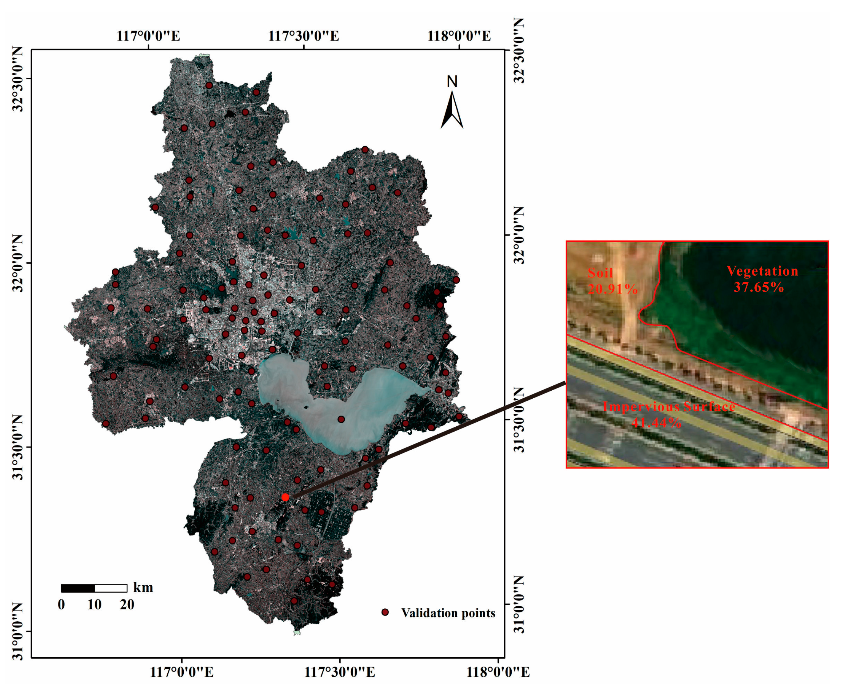
2. Study Area
3. Data and Methods
3.1. Data Collection
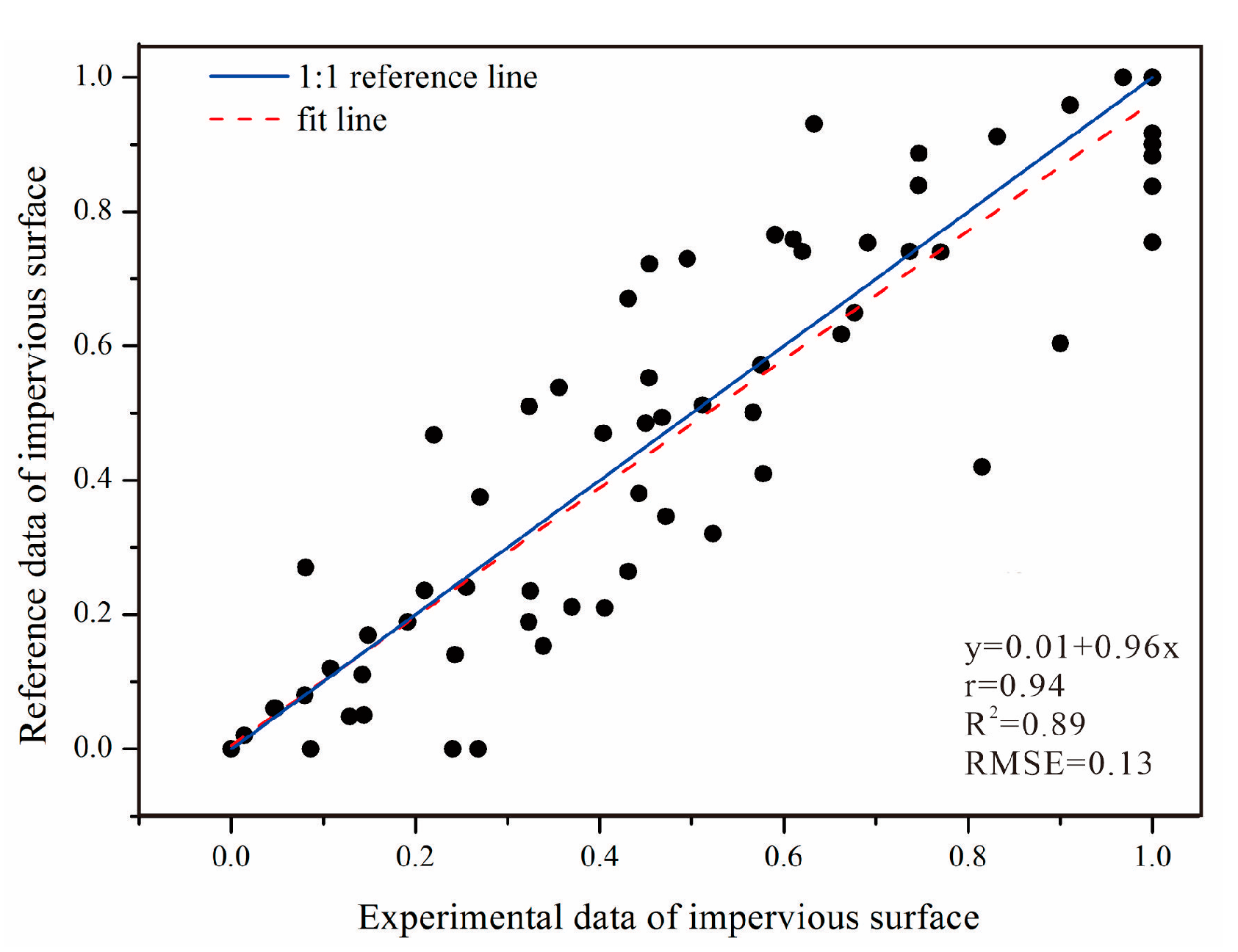
3.2. Mapping is Distribution and Validating the Results
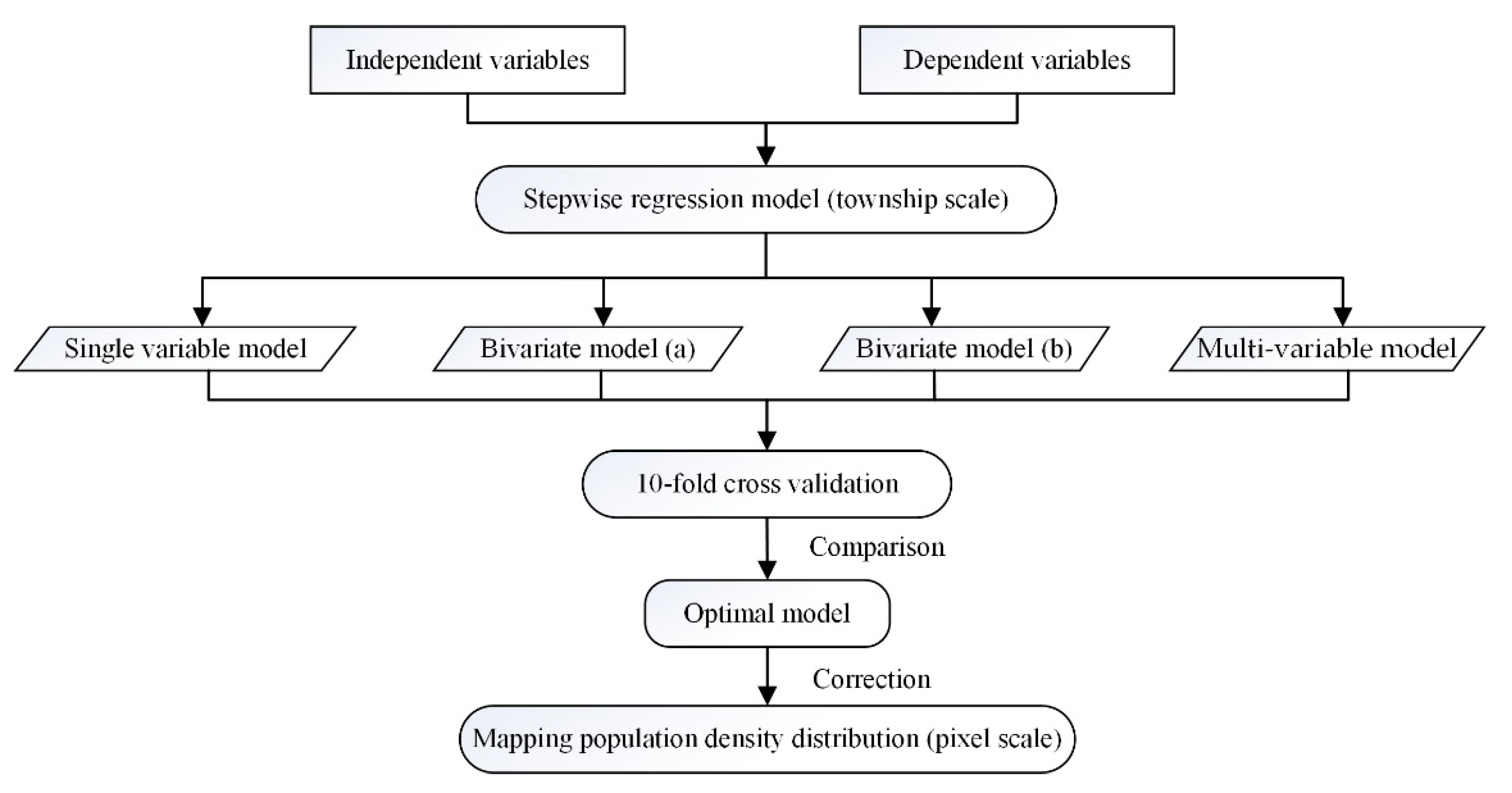
3.3. Modelling Population Density Estimation Using Stepwise Linear Regression
3.3.1. Data Preparation for Modelling
3.3.2. Model Concept and Validation
4. Results
4.1. Analysis of is Distribution and Assessment
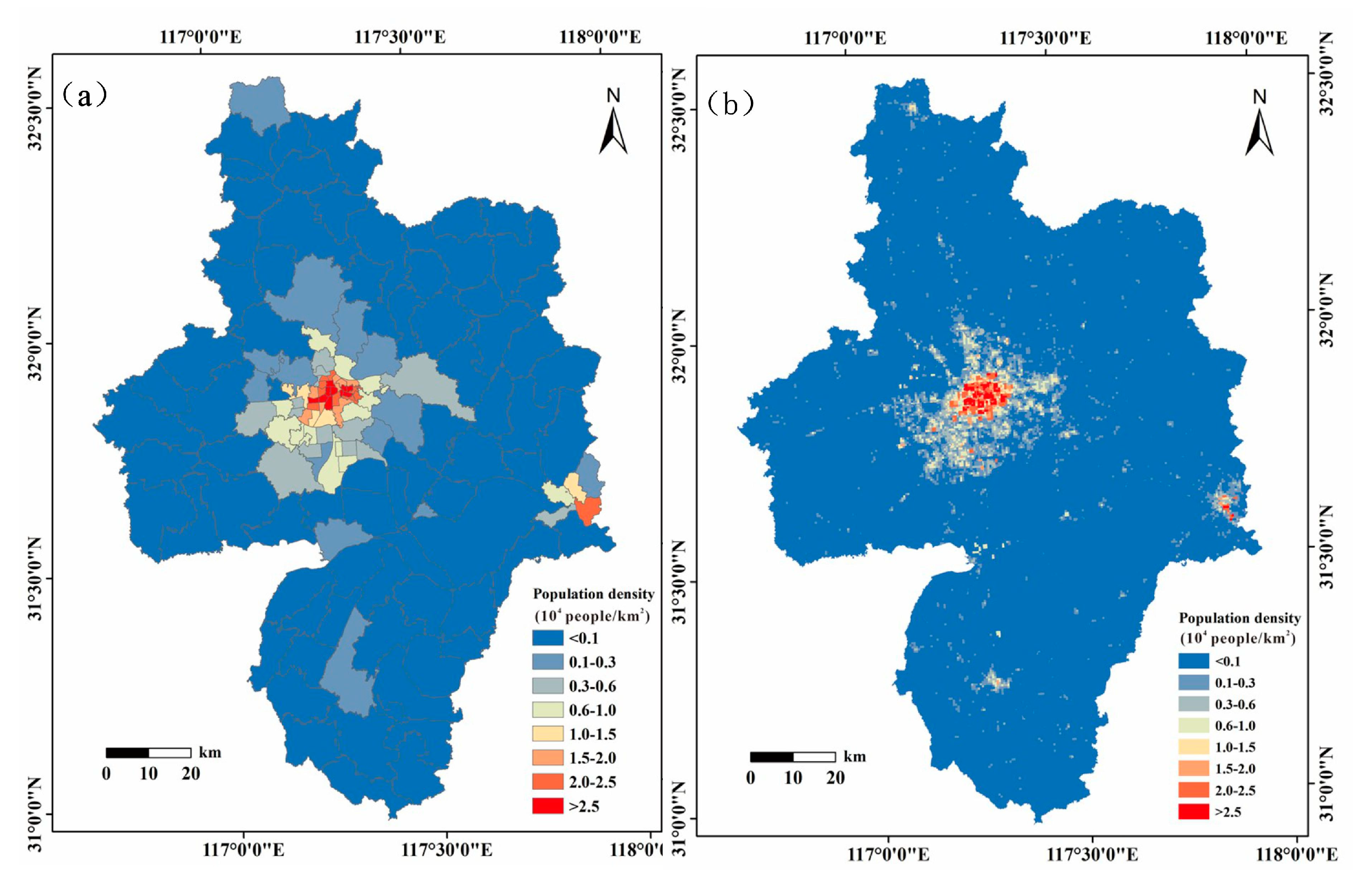
4.2. Stepwise Regression Models for Population Density Estimation
4.2.1. Correlation Analysis between Variables
4.2.2. Comparison and Validation of Models
5. Discussion
6. Conclusions
Author Contributions
Funding
Institutional Review Board Statement
Informed Consent Statement
Data Availability Statement
Acknowledgments
Conflicts of Interest
References
- Ciommi, M.; Egidi, G.; Salvia, R.; Cividino, S.; Rontos, K.; Salvati, L. Population dynamics and agglomeration factors: A non-linear threshold estimation of density effects. Sustainability 2020, 12, 2257. [Google Scholar] [CrossRef]
- Wu, S.S.; Qiu, X.; Wang, L. Population estimation methods in GIS and remote sensing: A review. GIScience Remote Sens. 2005, 42, 80–96. [Google Scholar] [CrossRef]
- Zhu, H.; Li, Y.; Liu, Z.; Fu, B. Estimating the population distribution in a county area in China based on impervious surfaces. Photogramm. Eng. Remote Sens. 2015, 81, 155–163. [Google Scholar]
- Li, L.; Lu, D. Mapping population density distribution at multiple scales in Zhejiang Province using Landsat Thematic Mapper and census data. Int. J. Remote Sens. 2016, 37, 4243–4260. [Google Scholar] [CrossRef]
- Lu, D.; Weng, Q.; Li, G. Residential population estimation using a remote sensing derived impervious surface approach. Int. J. Remote Sens. 2006, 27, 3553–3570. [Google Scholar] [CrossRef]
- Zhang, G.; Rui, X.; Poslad, S.; Song, X.; Fan, Y.; Wu, B. A method for the estimation of finely-grained temporal spatial human population density distributions based on cell phone call detail records. Remote Sens. 2020, 12, 1–28. [Google Scholar]
- Yang, X.; Ye, T.; Zhao, N.; Chen, Q.; Yue, W.; Qi, J.; Zeng, B.; Jia, P. Population mapping with multisensor remote sensing images and point-of-interest data. Remote Sens. 2019, 11, 574. [Google Scholar] [CrossRef]
- Mossoux, S.; Kervyn, M.; Soulé, H.; Canters, F. Mapping population distribution from high resolution remotely sensed imagery in a data poor setting. Remote Sens. 2018, 10, 1409. [Google Scholar] [CrossRef]
- Yu, S.; Zhang, Z.; Liu, F. Monitoring population evolution in China using time-series DMSP/OLS nightlight imagery. Remote Sens. 2018, 10, 194. [Google Scholar] [CrossRef]
- Jing, C.; Zhou, W.; Qian, Y.; Yan, J. Mapping the urban population in residential neighborhoods by integrating remote sensing and crowdsourcing data. Remote Sens. 2020, 12, 3235. [Google Scholar] [CrossRef]
- Xu, M.; Cao, C.; Jia, P. Mapping Fine-Scale Urban Spatial Population Distribution Based on High-Resolution Stereo Pair. Remote Sens. 2020, 12, 608. [Google Scholar] [CrossRef]
- Luo, P.; Zhang, X.; Cheng, J.; Sun, Q. Modeling population density using a new index derived from multi-sensor image data. Remote Sens. 2019, 11, 2620. [Google Scholar]
- Li, G.; Weng, Q.; Li, G.; Weng, Q. Fine-scale population estimation: How Landsat ETM + imagery can improve population distribution mapping. Can. J. Remote. Sens. 2014, 16, 8992. [Google Scholar] [CrossRef]
- Dong, P.; Ramesh, S.; Nepali, A. Evaluation of small-area population estimation using LiDAR, Landsat TM and parcel data. Int. J. Remote. Sens. 2010, 31, 1161. [Google Scholar] [CrossRef]
- Karunarathne, A.; Lee, G. Estimating Hilly Areas Population Using a Dasymetric Mapping Approach: A Case of Sri Lanka ’ s Highest Mountain Range. Int. J. Geo-Inf. 2019, 8, 166. [Google Scholar] [CrossRef]
- Hegedus, E. Population Estimation from Landsat Imagery. Remote Sens. Environ. 1982, 272, 259–272. [Google Scholar]
- Lo, C.P. Automated population and dwelling unit estimation from high-resolution satellite images: A GIS approach. Int. J. Remote. Sens. 2007, 1161, 16–34. [Google Scholar]
- Arnold, C.L.; Gibbons, C.J. Impervious Surface Coverage: The Emergence of a Key Environmental Indicator. J. Am. Plan. Assoc. 1996, 62, 243–258. [Google Scholar] [CrossRef]
- Zhou, Z.; Sha, J.; Ji, J. The Study of the Relationship between Urban Heat Island Effect and Impervious Surface and Spatio-temporal Change in Urban Areas of Fuzhou. J. Fujian Norm. Univ. 2019, 35, 24–32. [Google Scholar]
- Wang, X.; Xue, W.; Zhao, J. Sepctral Mixture Analysis and Mapping of Impervious Surface in Central Uran of Xi’an. Shaanxi. For. Sci. Technol. 2019, 47, 32–38. [Google Scholar]
- Cui, Q.; Pan, Y.; Yang, X. Beijing Plain Area of Remote Sensing Images Based on Landsat 8 Impervious Layer Coverage Estimates. J. Cap. Norm. Univ. 2015, 36, 89–92. [Google Scholar]
- Wu, C.; Murray, A.T. Population Estimation Using Landsat Enhanced Thematic Mapper Imagery. Geogr. Anal. 2007, 39, 26–43. [Google Scholar] [CrossRef]
- Joseph, M.; Wang, L.; Wang, F. Using Landsat Imagery and Census Data for Urban Population Density Modeling in Port-au-Prince, Haiti. GIScience Remote Sens. 2013, 49, 1603. [Google Scholar] [CrossRef]
- Xu, H.; Shi, T.; Wang, M.; Fang, C.; Lin, Z. Predicting effect of forthcoming population growth–induced impervious surface increase on regional thermal environment: Xiong’an New Area, North China. Build. Environ. 2018, 136, 98–106. [Google Scholar] [CrossRef]
- Azar, D.; Graesser, J.; Engstrom, R.; Comenetz, J.; Andrews, T. Spatial refinement of census population distribution using remotely sensed estimates of impervious surfaces in Haiti. Remote Sens. 2010, 31, 5635–5655. [Google Scholar] [CrossRef]
- Sugg, Z.P.; Finke, T.; Goodrich, D.; Moran, M.S.; Yool, S.R. Mapping Impervious Surfaces Using Object-oriented Classification in a Semiarid Urban Region. Photogramm Eng. Remote Sens. 2014, 80, 343–352. [Google Scholar] [CrossRef]
- Wu, C. Normalized spectral mixture analysis for monitoring urban composition using ETM + imagery. Remote. Sens. Environ. 2004, 93, 480–492. [Google Scholar] [CrossRef]
- Duan, P.; Li, J.; Lu, X.; Feng, C. Estimation of Impervious Surface Distribution by Linear Spectral Mixture Analysis: A Case Study in Nantong. In Proceedings of the 2nd EAI International Conference on Robotic Sensor Networks, Kunming, China, 25–26 August 2018; pp. 41–51. [Google Scholar]
- Li, L.; Lu, D.; Kuang, W. Examining urban impervious surface distribution and its dynamic change in Hangzhou metropolis. Remote Sens. 2016, 8, 265. [Google Scholar] [CrossRef]
- Liu, Q.; Sutton, P.C.; Elvidge, C.D. Relationships between Night Imagery and Population Density for Hong Kong. Proc. Asia-Pacific Adv. Netw. 2011, 31, 79. [Google Scholar]
- Zou, Y.; Yan, Q.; Huang, J.; Li, F. Modeling the Population Density of Su-Xi-Chang Region Based on Luojia-1A Night Light Image. Resour. Environ. Yangtze Basin 2020, 29, 1086–1094. [Google Scholar]
- Huang, X.; Yang, J.; Li, J.; Wen, D. Urban functional zone mapping by integrating high spatial resolution night light and daytime multi-view imagery. ISPRS J. Photogramm Remote Sens. 2021, 175, 403–415. [Google Scholar] [CrossRef]
- Zhao, M.; Zhou, Y.; Li, X.; Cheng, W.; Huang, K. Mapping urban dynamics (1992–2018) in Southeast Asia using consistent nighttime light data from DMSP and VIIRS. Remote Sens. Environ. 2020, 248, 111980. [Google Scholar] [CrossRef]
- Levin, N.; Kyba, C.; Zhang, Q.; Miguel, A.; Elvidge, C.D. Remote sensing of night lights: A review and an outlook for the future. Remote Sens. Environ. 2020, 237, 111443. [Google Scholar] [CrossRef]
- Gao, H.; Li, D.; Zhou, L.; Yu, T.; Huang, J. Population spatialization based on multiple night lighting data comparison. Intelligent City. 2020, 6, 26–27. [Google Scholar]
- Zhong, L.; Liu, X. Application potential analysis of LJ1-01 new nighttime light data. Bull. Surv. Mapp. 2019, 7, 132–137. [Google Scholar]
- Yin, J.; Fu, P.; Hamm, N.A.S.; Li, Z.; You, N.; He, Y.; Cheshmehzangi, A.; Dong, J. Decision-Level and Feature-Level Integration of Remote Sensing and Geospatial Big Data for Urban Land Use Mapping. Remote Sens. 2021, 13, 1579. [Google Scholar] [CrossRef]
- Chun, J.; Zhang, X.; Huang, J.; Zhang, P. A Gridding Method of Redistributing Population Based on POIs. Geogr. Geo-Inf. Sci. 2018, 34, 89–95. [Google Scholar]
- Chen, Y.; Ge, Y.; An, R.; Chen, Y. Super-Resolution Mapping of Impervious Surfaces from Remotely Sensed Imagery with Points-of-Interest. Remote Sens. 2018, 10, 242. [Google Scholar] [CrossRef]
- Zhao, Y.; Li, Q.; Zhang, Y.; Du, X. Improving the accuracy of fine-grained population mapping using population-sensitive POIs. Remote Sens. 2019, 11, 2502. [Google Scholar] [CrossRef]
- Feng, X.; Jin, Z. Belt and Road: An analysis based on Hefei. J. Suihua Univ. 2019, 39, 19–23. [Google Scholar]
- Xu, H. A Study on Information Extraction of Water Body with the Modified Normalized Difference Water Index (MNDWI). J. Remote. Sens. 2005, 9, 79–85. [Google Scholar]
- Small, C. The Landsat ETM+ spectral mixing space. Remote Sens. Environ. 2004, 93, 1–17. [Google Scholar] [CrossRef]
- Ridd, M.K. Exploring a V-I-S (Vegetation-impervious surface-soil) model for urban ecosystem analysis through remote sensing: Comparative anatomy for citiest. Int. J. Remote Sens. 1995, 16, 2165–2185. [Google Scholar] [CrossRef]
- Li, L.; Canters, F.; Solana, C.; Ma, W.; Chen, L.; Kervyn, M. Discriminating lava flows of different age within Nyamuragira’s volcanic field using spectral mixture analysis. Int. J. Appl. Earth Obs. Geoinf. 2015, 40, 1–10. [Google Scholar] [CrossRef]
- Cui, Y.; Li, L.; Chen, L.; Zhang, Y.; Cheng, L.; Zhou, X.; Yang, X. Land-use carbon emissions estimation for the Yangtze River Delta Urban Agglomeration using 1994-2016 Landsat image data. Remote Sens. 2018, 10, 1334. [Google Scholar] [CrossRef]
- Lin, Y.P.; Chu, H.J.; Wu, C.F.; Chang, T.K.; Chen, C.Y. Hotspot analysis of spatial environmental pollutants using kernel density estimation and geostatistical techniques. Int. J. Environ. Res. Public Health 2011, 8, 75–88. [Google Scholar] [CrossRef] [PubMed]
- Chainey, S. Examining the influence of cell size and bandwidth size on kernel density estimation crime hotspot maps for predicting spatial patterns of crime. Bull. Geogr. Soc. Liege 2013, 60, 7–19. [Google Scholar]
- Gatrell, A.C.; Bailey, T.C.; Diggle, P.J.; Rowlingson, B.S. Spatial point pattern analysis and its application in geographical epidemiology. Trans. Inst. Br. Geogr. 1996, 21, 256–274. [Google Scholar] [CrossRef]
- Nahler; Gerhard Pearson correlation coefficient. Springer Vienna 2009, 10, 132.
- Finn, J.D. A General Model for Multivariate Analysis; Holt Rinehart Winst: New York, NY, USA, 1974; pp. 173–174. [Google Scholar]
- Li, L.; Zhou, X.; Chen, L.; Chen, L.; Zhang, Y.; Liu, Y. Estimating urban vegetation biomass from sentinel-2A image data. Forests 2020, 11, 125. [Google Scholar] [CrossRef]
- Abdelhafidi, N.; Bachari, N.E.I.; Abdelhafidi, Z. Estimation of solar radiation using stepwise multiple linear regression with principal component analysis in Algeria. Meteorol. Atmos. Phys. 2020, 133, 1–12. [Google Scholar] [CrossRef]
- Nouman, S. Multiple and stepwise regression of reproduction efficiency on linear type traits in Sahiwal cows. Int. J. Livest. Prod. 2013, 4, 14–17. [Google Scholar] [CrossRef][Green Version]
- Zhou, Y.; Qureshi, R.; Sacan, A. Analysis of paired miRNA-mRNA microarray expression data using a stepwise multiple linear regression model. Lect. Notes Comput. Sci. 2017, 10330, 59–70. [Google Scholar]
- Li, L.; Bakelants, L.; Solana, C.; Canters, F.; Kervyn, M. Dating lava flows of tropical volcanoes by means of spatial modeling of vegetation recovery. Earth Surf. Process. Landforms. 2018, 43, 840–856. [Google Scholar] [CrossRef]
- Yuan, L.; Li, L.; Zhang, T.; Chen, L.; Liu, W.; Hu, S.; Yang, L. Modeling Soil Moisture from Multisource Data by Stepwise Multilinear Regression: An Application to the Chinese Loess Plateau. ISPRS Int. J. Geo-Inf. 2021, 10, 233. [Google Scholar] [CrossRef]
- Wu, C.; Murray, A.T. Estimating impervious surface distribution by spectral mixture analysis. Remote Sens. Environ. 2003, 84, 493–505. [Google Scholar] [CrossRef]
- Zou, Y. Research on Population Spatialization Based on Multi-Source Data. Master’s Thesis, China University of Mining and Technology (Jiangsu), Xuzhou, China, 2020. [Google Scholar]
- He, M.; Xu, Y.; Li, N. Population Spatialization in Beijing City Based on Machine Learning and Multisource Remote Sensing Data. Remote Sens. 2020, 12, 1910. [Google Scholar] [CrossRef]
- Li, H.; Li, L.; Chen, L.; Zhou, X.; Cui, Y.; Liu, Y.; Liu, W. Mapping and characterizing spatiotemporal dynamics of impervious surfaces using landsat images: A case study of Xuzhou, East China from 1995 to 2018. Sustainability 2019, 11, 1224. [Google Scholar] [CrossRef]
- Xu, Z.; Ouyang, A. The Factors Influencing China’s Population Distribution and Spatial Heterogeneity: A Prefectural-Level Analysis using Geographically Weighted Regression. Appl. Spat. Anal. Policy. 2018, 11, 465–480. [Google Scholar] [CrossRef]
- Mi, R.; Gao, X. Factors influencing population distribution in Shaanxi Province using spatial econometric analysis. Arid Land Geogr. 2020, 43, 491–498. [Google Scholar]


| Data Sources | Description |
|---|---|
| Landsat imagery | Path 121 and row 38 on 10 April 2018, cloudiness of 0.03 |
| POI data | 123,348 points related to population from Baidu Map of Hefei in 2018 |
| NTL data | Night light data from Luojia-1 satellite of Hefei in 2018 |
| Population data at township scale | 141 townships of Hefei based on the census in 2018 |
| Administrative data | Boundary vector at township scale |
| IS Data | POI Data | NTL Data | |
|---|---|---|---|
| IS data | 1 | 0.729 *** | 0.689 *** |
| POI data | 1 | 0.673 ** | |
| NTL data | 1 |
| IS Data | POI Data | NTL Data | |
|---|---|---|---|
| IS data | 0.495 *** | 0.391 *** | |
| POI data | 0.495 *** | 0.345 *** | |
| NTL data | 0.391 *** | 0.345 *** |
| Single Variable Model | Bivariate Model (a) | Bivariate Model (b) | Multi-Variable Model | |
|---|---|---|---|---|
| IS data | 7.922 *** | 6.700 *** | 5.582 *** | 4.567 *** |
| POI data | 2.515 *** | 1.497 *** | ||
| NTL data | 2.317 *** | 2.932 *** | ||
| Constant | 4.983 *** | 5.125 *** | 5.325 *** | 5.402 *** |
| Max VIF | 1.000 | 2.438 | 2.916 | 2.989 |
| Training Group | Validation Group | ||||
|---|---|---|---|---|---|
| Types of Models | Adj.R2 | RMSE | Adj.R2 | RMSE | MAE |
| Single variable model | 0.687 | 0.940 | 0.689 | 0.922 | 0.687 |
| Bivariate model (a) | 0.711 | 0.847 | 0.715 | 0.910 | 0.661 |
| Bivariate model (b) | 0.834 | 0.685 | 0.834 | 0.686 | 0.514 |
| Multi-variable model | 0.856 | 0.633 | 0.852 | 0.632 | 0.460 |
Publisher’s Note: MDPI stays neutral with regard to jurisdictional claims in published maps and institutional affiliations. |
© 2021 by the authors. Licensee MDPI, Basel, Switzerland. This article is an open access article distributed under the terms and conditions of the Creative Commons Attribution (CC BY) license (https://creativecommons.org/licenses/by/4.0/).
Share and Cite
Zang, J.; Zhang, T.; Chen, L.; Li, L.; Liu, W.; Yuan, L.; Zhang, Y.; Liu, R.; Wang, Z.; Yu, Z.; et al. Optimization of Modelling Population Density Estimation Based on Impervious Surfaces. Land 2021, 10, 791. https://doi.org/10.3390/land10080791
Zang J, Zhang T, Chen L, Li L, Liu W, Yuan L, Zhang Y, Liu R, Wang Z, Yu Z, et al. Optimization of Modelling Population Density Estimation Based on Impervious Surfaces. Land. 2021; 10(8):791. https://doi.org/10.3390/land10080791
Chicago/Turabian StyleZang, Jinyu, Ting Zhang, Longqian Chen, Long Li, Weiqiang Liu, Lina Yuan, Yu Zhang, Ruiyang Liu, Zhiqiang Wang, Ziqi Yu, and et al. 2021. "Optimization of Modelling Population Density Estimation Based on Impervious Surfaces" Land 10, no. 8: 791. https://doi.org/10.3390/land10080791
APA StyleZang, J., Zhang, T., Chen, L., Li, L., Liu, W., Yuan, L., Zhang, Y., Liu, R., Wang, Z., Yu, Z., & Wang, J. (2021). Optimization of Modelling Population Density Estimation Based on Impervious Surfaces. Land, 10(8), 791. https://doi.org/10.3390/land10080791