Pan-European Mapping of Underutilized Land for Bioenergy Production

Abstract

This study aims at identifying underutilized land potentially suitable for bioenergy production in Europe by means of remote sensing time series analysis. The background is the Revised Renewable Energy Directive (REDII) requesting that 32% of Europe’s energy production shall come from renewable energy sources until 2030. In order to avoid the food versus fuel debate, we only considered land that has not been used in the previous five years. Satellite remote sensing is the only technique that allows for the assessment of the usage of land for such a long time span at the pan-European scale with reasonable efforts. We used Landsat 8 (L8) data for the full five year time period 2015–2019 and included additional Sentinel-2 (S2) data for 2018 and 2019. The analysis was based on a stratified approach for biogeographical regions and countries using Google Earth Engine. To our knowledge, this is the first work that employs high resolution time series data for pan-European mapping of underutilized land. The average patch size of underutilized land was found to be between 23.2 ha and 49.6 ha, depending on the biogeographical region. The results show an overall accuracy of more than 85% with a confidence interval (CI) of 1.55% at the 95% confidence level (CL). The classification suggests that at total of 5.3 million ha of underutilized land in Europe is potentially available for agricultural bioenergy production.

1. Introduction

According to the REDII, 32% of the energy production in the EU should come from renewable energy sources until 2030 [1]. To reach this aim, one option is to use bioenergy as a renewable energy source [2]. This study is embedded in the Horizon 2020 project BIOPLAT-EU with the overall goal to promote the market uptake of sustainable bioenergy in Europe using marginal, underutilized, and contaminated lands for non-food biomass production through the provision of a web-based platform that serves as a decision support tool (www.bioplat.eu).

Following the REDII, various related studies [3,4] suggest positive impacts of bioenergy on, for example, economic opportunities for farmers, climate change mitigation, increased energy security, and additional employment option in rural areas. However, bioenergy production, and in particular large-scale investment in advanced bioenergy production, still fall through because of a lack of acceptance by the public, mainly due to two major issues: first, the environmental, social, and economic sustainability of bioenergy supply chains; and second, existing technical, financial, political, and legal market uptake barriers. In this part of the work we focus on the first issue. Environmental, social, and economic impacts of bioenergy production are manifold and have been assessed in various studies [5,6]. Especially the potential disruption of food security has become a major concern, often termed as a “food versus fuel issue”. Other concerns, such as water scarcity and impacts on the ecological balance and/or on biodiversity or potential displacement of small-scale farmers have been noted [6].

The BIOPLAT-EU project dealt with these controversial issues in two ways. First, the food versus fuel issue was avoided by focusing on land that (i) had not been used in the last 5 years (underutilized land, UU), or (ii) could not be used for food production due to contamination. This was the basis of the BIOPLAT-EU’s methodology to assess the land available to grow agricultural biomass for bioenergy. Second, potential negative impacts are assessed using a sustainability assessment tool (Sustainability Tool for Europe and Neighboring countries (STEN)), which is based on the methodologies developed by the Food and Agriculture Organization of the United Nations (FAO) in the context of the previous H2020 project “Fostering Sustainable Feedstock Production for Advanced Biofuels on underutilized land in Europe (FORBIO)”. The STEN tool assesses the sustainability of the potential bioenergy value chains measuring the impact of the envisaged bioenergy production against specific sustainability indicators. The roots of its methodologies are the recognized Global Bioenergy Partnership (GBEP) sustainability indicators (GSI) from which the FORBIO’s sustainability indicators have been adapted. The knowledge of datasets, reference default values, metrics, and units of a series of existing and available databases were essential to further develop STEN into an automated calculator for assessing bioenergy sustainability. The impact is calculated as the difference between the situation “as-is” and the projections considering the realization of a bioenergy project. The specific structure of the STEN’s information flow allows advanced users to modify default data from the databases to temporarily build and handle a user-tailored database that better fits the scope of a given analysis. Upon completion, the webGIS, including the underutilized land map and the STEN tool, will be available through the project website (www.bioplat.eu).

While in BIOPLAT-EU both underutilized and contaminated lands are considered, this paper focuses only on identifying available underutilized lands. For the identification of these lands, the official FAO time span of abandoned farmland was adopted. In FAO’s World Census of Agriculture, FAO 2020, Art. 8.2.24 states: “Land remaining fallow for too long may acquire characteristics requiring it to be reclassified, such as ‘permanent meadows and pastures’ (if used for grazing), ‘forest and other wooded land’ (if overgrown with trees), or ‘other land’ (if it becomes wasteland). A maximum idle period should be specified—five years is usually suitable. Land cultivated on a two- or three-year rotating basis is considered to be fallow if it was not cultivated during the reference year. Land temporarily fallow should be distinguished from land abandoned by shifting cultivation; the former is part of the holding, whereas the latter is not.” Since not only abandoned farmland is considered but rather all underutilized land, we extended the definition to “all land that does not show any signs of human use for the past five years”. In order to assess the existence of signs of human use, we employed time series of remotely sensed data from Copernicus and other Earth Observation programs.

Previous studies on the classification of underutilized or abandoned (farm-) land using Earth Observation data mainly concentrate on Eastern Europe, where large agricultural areas had been abandoned after the breakdown of communist agricultural structures. Studies used either high-temporal and low spatial resolution data such as MODIS [7,8,9], or existing data bases such as CORINE land cover (CLC), which can be considered as an indirect remote sensing approach [10]. MODIS data was also used for large-area assessments in Asia [11,12] proving to be well suited for identifying large and homogeneous underutilized areas on a continental scale. MODIS has a spatial resolution of 500 m pixel size on the ground, resulting in related minimum mapping units. In [12], for example, the minimum pixel size is 10 arc-seconds, which is approximately 4–7 hectares. This is absolutely sufficient for a trans-Asian assessment. However, considering the small structured agricultural lands in large parts of Europe, this sensor is simply too coarse to produce the high-resolution results needed, as many potentially interesting areas would not be detectable.

Existing European studies on the national or regional scale typically used low temporal and high spatial resolution data, such as in Slovakia [13,14]. To map post-socialism farmland abandonment at the regional level in Western Ukraine, the authors in [15] employed Landsat time series data from 1986 until 2008. Other investigations combined high spatial resolution satellite data with existing databases in Europe, e.g., in Italy [2].

The aim of this study is thus to bridge the gap between continental assessment and high-resolution mapping requirements by employing Landsat and Sentinel-2 time series data for EU and selected neighboring countries. Landsat 8 data with a spatial resolution of 30 m was selected as the main data source in order to fulfil the definition of underutilized land (past five years), when the assessment started in 2019. Sentinel-2 with a spatial resolution of 10 m could only be used as an additional data source, since the first Sentinel-2 images became available only in 2016. The mapping was realized using Google Earth Engine (GEE) [16].

The working hypothesis is that underutilized (UU) land has a different spectral reflectance behavior over time compared to utilized (U) land due to missing human interventions. Typical human interventions are mowing and ploughing, which result in clear changes in the spectral reflectance of the respective patch of land. It is assumed that UU land shows smaller magnitudes and lower standard deviations of changes over time than utilized land due to missing above-mentioned interventions.

2. Study Area and Data

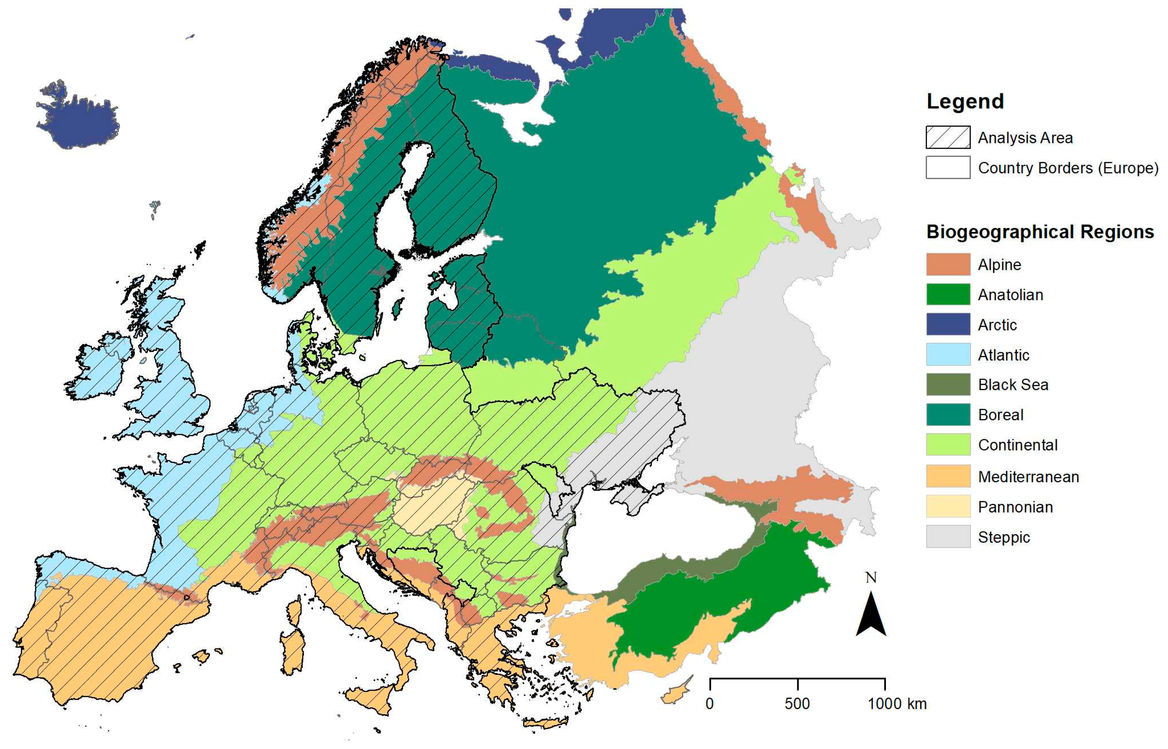
2.1. Study Area

The study area comprised the EU and selected neighboring countries (see Figure 1). Ukraine, for example, was included because of its known potential for underutilized areas, which could be used for the European bioenergy market. The classification was performed in a stratified manner dividing the study area by (1) biogeographical regions of Europe [17] provided by the European Environmental Agency (EEA) [18], and (2) countries. The first stratification was done due to the different climatic situations throughout Europe, which cause UU land to have very different properties in different regions. The mean annual precipitation plays a significant role here, but the minimum and maximum temperature and the elevation are also important factors. This leads to significant differences in spectral phenological profiles of the same land use class in different regions of Europe, which is also applicable to underutilized lands. Figure 2 shows an example of spectral profiles of underutilized lands for different biogeographical regions. By using biogeographical regions to stratify the classification, these differences are taken into account.

The second stratification (by country) was done for technical and practical reasons: first, without it, the size of some areas would be too large for processing (system running out of memory), and second, the handling of data on a country-by-country basis is an agreement within the BIOPLAT-EU project.

2.2. Data

2.2.1. Satellite Imagery

Generally, optical Earth Observation (EO) data, provided as multi-spectral images, captures comprehensive information about reflection characteristics of the Earth’s surface. This makes them very suitable for land cover and land use (LCLU) studies [19]. The Landsat 8 (L8) satellite was launched on 11 February 2013. It has a global revisit time of 16 days and delivers comprehensive images of the earth’s surface between 57° S and 84° N. On board, L8 carries the Operational Land Imager (OLI), which has nine spectral bands that cover the electromagnetic spectrum from the visible to the short-wave infrared domain (see Figure 3) and a spatial resolution of 30 m, except for the panchromatic band with 15 m resolution [20]. On its way from the sun to the earth’s surface, where it is reflected and further transmitted to the sensor, the electromagnetic radiation is additionally influenced by the atmosphere. However, land surface studies need image data whose pixel values provide reflectance information of the earth’s surface to ensure reliability. Therefore, Landsat 8 data is also available as a so-called Level 2 product, where these digital numbers are transformed to surface reflectance (SR) values for all bands, and another three bands are added that provide information about clouds, cloud and cirrus cloud confidence, cloud shadow, snow/ice and water pixel saturation, and the quality of aerosol retrieval [21].

Since 2008, the Landsat Program has been supporting an open data policy making the whole Landsat image archive accessible free of charge. Free access and duration of the whole mission make Landsat images one of the most used satellite data sources for mapping and monitoring of LCLU dynamics based on image time series [20,22]. To meet the BIOPLAT-EU definition of underutilized land, Landsat time series data from 2015 until 2019 was used as the main data source for the classification.

Within the frame of the Copernicus Program, the European Space Agency (ESA) launched the Sentinel-2 (S2) missions to provide high resolution dense optical time series data for the development of EO-based environmental monitoring systems [23]. S2 images have a spatial resolution of up to 10 m and are provided with a temporal resolution of 5 days [24]. The whole S2 system has been fully operational since mid-2017, delivering data from two satellites with 13 spectral bands (Figure 3). Recalling the need for a five year period to assess usage, it was not feasible to conduct our analysis solely based on S2 data. However, we integrated an S2 time series from 2018 and 2019 to generate a cropland mask to refine the classification result based on L8 data.

2.2.2. Reference Data for Training

Training data that represent “ground truth” are a crucial component in any remote sensing-based classification. Due to the pan-European set up of this study, the training data does not only have to represent all characteristics of underutilized lands but also all types of used land to set-up a classifier that is able to distinguish between underutilized and utilized. As mentioned in Section 2.1., in the case of European-wide underutilized land mapping, it needs to be considered that these lands can have a wide range of different characteristics. The training data sets were generated with the help of existing data sets such as “Land Use/Cover Area frame statistical Survey” (LUCAS) (point data); Copernicus High Resolution Layers (HRL) for forest, settlement, and water and wetness; and CORINE land cover data and were complemented with national data upon availability.

Since European-wide LCLU data sets are usually status products (e.g., they represent the LCLU of a certain point in time), they are only useable to point to potentially underutilized lands. The LUCAS database in particular has proven to be extremely valuable for the identification of training data. LUCAS is a harmonized in situ (terrestrial) LCLU data collection procedure. Details and the data sets can be obtained from the Eurostat Website (https://ec.europa.eu/eurostat/web/lucas/data/primary-data). LUCAS is done every three years, with the most recent survey in 2018.

For the purpose of classifying underutilized lands, LUCAS points which are assigned the LU classes U410 “Abandoned Areas” and U420 “Semi-Natural and Natural Areas not in Use” and do not belong to land cover classes water areas, wetland, woodland, or artificial land are of particular interest.

The direct use of LUCAS data for training purposes is, however, limited by 4 factors:

• The limited spatial extent per observation: “The “point” (or basic unit of observation) is in fact a circle with a radius of 1.5 m corresponding to an identifiable point on an orthophoto. As we have not only homogeneous classes that we would like to observe, for example forests (forest definition requires observing a certain area to define the crown coverage or canopy of the trees) or orchards (which may consist in more than one tree species, etc.), the LUCAS observation framework also specifies an observation area, the “extended window of observation” which is the area defined by a 20 m radius around the point, for specific classes.” [1].
• The point grid was not the same for all surveys, thus sometimes, there is only land use information for a specific year (e.g., 2015), but no information about the land use before or after.
• Sometimes a shift in the location between the same points can be observed in two different surveys.
• The last survey was conducted in 2018; the classification is done using image time series data from 2015 to 2019.

For these reasons, the selected relevant points with the above-mentioned land use classes were not directly used but were additionally analyzed visually using time series VHR image data available in Google Earth. In addition to the confirmation or rejection of the point itself, the interpreters also digitized the surrounding area with the same characteristics in case a point was confirmed to be underutilized. In total, 4000 LUCAS points were analyzed and 1971 polygons were generated.

For the compilation of a training data set that covers all types of used land, the following European-wide COPERNICUS Land Monitoring Service Products were used:

• High Resolution Layers (HRL) Forest, Imperviousness, and Water and Wetness
• CORINE Land Cover (CLC) 2018 agriculture classes “Arable land” (21), “Permanent crops” (22), and “Pastures” (23).

Due to their European-wide coverage, no further visual interpretation was needed to compile training data sets for the used land categories.

2.2.3. Data for Masking Specific Areas

Following the preconditions laid out in the introduction with regards to avoiding food versus fuel problems, we excluded certain areas from further assessment. These lands were identified with existing pan-European data sets, and the analysis was limited to all areas not covered by these data sets. The specific areas not to be considered included:

• Forest areas (HRL Forest): Forest areas are considered to be used land. Changing forests to other land use types is usually critical in terms of carbon balance [26] and was therefore avoided. Especially in Eastern Europe and former Soviet Union countries, young forests are growing on abandoned agricultural farmland [27,28]. The re-cultivation of these lands is a major issue of discussion [29,30]. However, since forest areas provide higher potential for carbon sequestration, we do not consider these areas as “underutilized land”.
• Settlement areas (HRL Imperviousness, Open Street Map (OSM), and CORINE land cover): Settlements belong to the category of used land.
• Water and Wetland areas (HRL Water and Wetness): In addition to excluding water bodies, wetland areas were removed for two reasons: first, due to limitations in drivability for mechanized growing of bioenergy crops, and second, due to the high natural value and biodiversity potential entailed in wetlands [31].
• Protected areas (Natura2000): Protected areas are removed totally, although the consortium is aware that crops used for energy might be allowed in some protected areas (e.g., outer zones of national parks). However, due to missing European-wide spatial separation between allowed and restricted zones, all areas are removed to avoid critical land competition.
• Steep slopes (>15° slope in Shuttle Radar Topography Mission digital elevation model (SRTM)): Steep slopes with inclinations larger than 15° are also removed because mechanized land cultivation is typically not feasible.
• Other not usable areas (CORINE land cover): Other not usable areas like beaches, bare rocks, or glaciers (CLC classes 331, 332 and 335) are also eliminated.
• Areas permanently used for agriculture (CORINE land cover): From the agriculturally used areas, most classes (CLC classes 221, 222, 223, 231, 241, 242, and 244) are removed. The annual crops in CORINE land cover (CLC classes 211, 212, and 213) are not removed in order to detect abandoned farmlands.

As the Copernicus high resolutions layers CLC and Natura2000 products do not cover Ukraine, suitable substitutes had to be found. For LCLU, a map produced within research activities for a doctoral thesis [32] could be used to substitute HRL and CLC. The following LCLU classes are differentiated in this map: forest, water, wetlands, cropland, grassland, scrubland, settlements, and other land. In order to eliminate protected areas within Ukraine, the official cadastral information (https://map.land.gov.ua/) was used. Areas assigned to “national or nature parks”, “nature reserves”, “RAMSAR sites”, and “nature conservation areas” were eliminated. All these areas were merged to an “elimination mask”, which was cut out of the study area, and the remaining areas were termed as “area of interest”.

Table 1. Calculation of the area of interest.

Biogeographical Region	Study Area (ha)	Elimination Mask (ha)	Area of Interest (ha)
Alpine	63,815,477	50,898,030	12,917,447
Atlantic	86,135,597	53,133,180	33,002,417
Boreal	89,317,815	60,034,485	29,283,330
Continental	173,990,564	93,346,118	80,644,446
Mediterranean	92,181,777	59,869,101	32,312,676
Pannonian	12,901,241	5,121,331	7,779,910
Steppic	28,226,727	6,233,216	21,993,511
Overall	546,569,198	328,635,461	217,933,737

provides information on the elimination mask and area of interest. Most of the study area lies within the continental region, while the Pannonian region has the smallest share. As to be expected, the area of interest of the Alpine region is the smallest in relation to the total area of this biogeographical region; almost 80% of the area was excluded from the analysis. Similarly, from the Boreal region more than two thirds of the total area was not considered, mainly due to the large extent of Boreal forests. Overall, about 40% of the whole study area was included in the classification process.

3. Methodology

The methodology chapter is subdivided into two sections. Section 3.1. explains the classification method. It should be noted that the classification was done for the area of interest (not the elimination mask). Section 3.2. details the methods for validation of the results including the tricky issue of generating a ground truth data set for a duration of five years and the problems entailed in using VHR data for validating HR results.

3.1. Method for the Classification of Underutilized Land

The entire mapping approach is schematically depicted in Figure 4. Classification on a continental scale with high resolution time series data is demanding both in terms of covering all different variations (see Figure 2) as well as in terms of data handling. To facilitate the data handling and processing, the satellite image classification was performed using Google Earth Engine (GEE). GEE is an online cloud-based processing engine for geospatial analyses, available free of charge for research projects. User access is provided through an internet-accessible application programming interface (API) and an associated interactive development environment. Through client libraries available for JavaScript and Python programming languages, it offers all necessary tools for geospatial analyses and visualization (maps and graphs). Since GEE has a wide user group sharing their work, a lot of pre-defined functions and processing workflows are available [16]. Another reason for GEE’s popularity is the extensive amount of available data easily accessible and ready-to use. Additionally, each user can upload his/her own data sets to a private storage space and integrate them into analyses [16].

As explained in Section 2.2, Landsat 8 Level 2 SR data was employed. Since L8 is an optical sensor, it has the disadvantage that it cannot “see” through clouds. Hence, an image might have cloudy pixels that do not represent the actual reflectance of the earth’s surface. This leads to outliers in the temporal trajectory when image time series analysis is performed and, subsequently, misclassifications might occur. To overcome this issue, the pixel quality band (qa) [33] was used to eliminate clouds in images.

Generally, when image classification is performed, it is beneficial to use those input features (spectral bands, indices, etc.) that best capture the spectral differences between the response variables (e.g., LCLU classes). Nowadays a lot of classifiers are able to handle high dimensional data sets (large numbers of input features) and can extract the most relevant features internally during classification procedures. However, if computational resources are limited and the size of the area is as large as in this study, it is still beneficial to ensure effective and efficient classification performance by reducing the amount of input data used beforehand. For this feature reduction, existing knowledge was considered, e.g., the band 2 (blue) was omitted due to the strong influence of aerosols on reflectance in this domain of the electromagnetic spectrum, and also band 7 (short wave infrared—swir2) was not considered due to similar spectral behavior of vital vegetation in both swir bands. Furthermore, the image time series was reduced to the growing season. From the remaining bands and possible vegetation indices, those already proven to support modelling of vegetation phenology in previous studies [34,35,36,37,38,39] were used:

• B3 (green)
• B4 (red)
• B5 (nir)
• B6 (swir1)
• NDVI (normalized difference vegetation index)
• NDII5 (normalized difference infrared index)
• MCARI (modified chlorophyll absorption in reflectance index) [40]
• MSAVI (modified soil-adjusted vegetation index) [41]

From each of these bands, monthly statistic images (minimum, maximum, standard deviation, percentiles; see details below) were calculated. This had to be done for two reasons: first, to reduce the amount of data for performance reasons, and second, to reduce the number of “no data” (ND) pixels. These are pixels that carry no valid spectral information due to the cloud masking algorithm applied. ND pixels pose a problem to the follow-up random forest classifier (see below) and should therefore be eliminated or at least minimized. In terms of statistical values used for the generation of the monthly images, we used either minimum or maximum, depending on the band/index, in order to capture certain spectral responses typical for mowing or ploughing events that indicate human-induced activities. Minimum pixel values were calculated for B3, B5, NDVI, NDII5, MSAVI, and MCARI. Maximum pixel values were used for B4 and B6. However, especially during bad weather periods in combination with the Landsat system’s repeat rate of only 16 days, sometimes no valid data are acquired for a whole month. Therefore, monthly statistics images still have ND pixels that cause problems for random forest classification. To overcome this issue, the following temporal statistics for the 5 year period were calculated for each of the selected bands and indices in order to test our hypothesis:

• minimum
• maximum
• standard deviation
• percentiles (10 and 90)

This resulted in a data set of 40 input features for the random forest (RF) classification. RF is a classification method that belongs, along with other boosting and bagging methods as well as classification trees in general, to the ensemble learning methods, which generate many classifiers and aggregate their results to calculate their response [42,43,44]. The random forest classifier integrates a set of independent decision trees to model the relationship between predictor (e.g., surface reflectance values, NDVI, temporal metrics, etc.) and response variable (e.g., utilized or underutilized) and can handle high dimensional continuous, categorical, and binary data sets [43,45,46,47]. The random forest algorithm offers good prediction performance and is computationally effective. Regarding the classifier’s sensitivity to the sample design and imbalanced training samples, different studies revealed contradictory results. The algorithm fails to cope with imbalanced training data, tending to favor the most representative class at the expense of the minority class [29]. Thus, at each sample selection at each node during the tree construction, fewer samples of the minority class are chosen [48]. On the contrary, other authors [45,49] found out that the random forest algorithm is less sensitive to outlier training samples or noisy data. The impact of several sampling designs on decision tree algorithms was tested [31], and recommendations include the area-proportional allocation to achieve the best classification results because classes occupying larger areas need more training samples.

In order to map human-induced activities such as mowing or ploughing, the NDVI standard deviation of the growing season was found to be particularly useful. Figure 5 shows that the standard deviation of the NDVI was clearly higher for annual crops and for managed grasslands than for underutilized grassland in the continental biogeographical region. The initially tested growing season was April to October, which turned out to give many false positives due to remaining snow cover or delay in spring vegetation in April, on the one hand, or early cold periods leading to discoloration of leaves in October, on the other. These effects generated similar high standard deviation values for pastures, underutilized lands, and annual crops. Therefore, the acquisition period was adapted from the beginning of May until the end of September. Still, with this approach, misclassifications occurred when no observations could be acquired for a whole month due to persistent cloud cover. After this period passed, the spectral response to the typical human usage such as mowing or tilling was lost and thus could not be properly detected.

In order to reduce this error, we included a final post-processing step using Copernicus Sentinel-2 SR data from the past two years of the targeted time span (right part in the workflow Figure 4). Of course, S2 data also contain ND values due to clouds. However, due to the much better temporal resolution of S2 compared to L8 the time delay until the next valid observation is much shorter, immensely improving the possibility of detecting human-induced activities in the time series. We used the GEE cloud masking algorithm for S2, making use of the additional “QA_60” band. Based on this pre-processing, the standard deviation of the NDVI over the past two years was calculated. All areas with a maximum standard deviation exceeding 0.17 were considered to have been ploughed at least once during this time and thus removed from the L8-based “underutilized land” class. The threshold was found through analysis of existing arable land patches.

The resulting classification was downloaded in raster format from GEE for further local post-processing. The main step was the application of a minimum mapping unit (MMU) of 10 ha, which was found to be good trade-off between spatial detail, sufficient size to be profitable, and European-wide assessment. Identified underutilized lands with areas smaller than 10 ha were discarded. Additionally, gaps inside underutilized lands smaller than 1 ha were closed, and the shapes of the polygons were simplified by applying the “eliminate polygon part”, “smooth polygon”, and “simplify polygon” GIS operations to avoid large amounts of complex polygons that would impede further data usage in the frame of the project.

3.2. Method for Validation of the Results

In order to generate a validation data set that allows accuracy assessments for the overall area of interest as well as for the area of interest within a single biogeographical region, a stratified random sampling approach as proposed by [50] was used. This approach takes into account the total mapped area as well as the mapped area per class, thus allowing us to also report—alongside the accuracy values—the confidence intervals (CIs) at 95% CL. For that reason, the classification result was divided into 14 sub-classes, e.g., utilized land in Alpine region, underutilized land in Alpine region, utilized land in Atlantic region, and so on.

In the first step, the overall available amount of validation points (in terms of resources) was subdivided into the 14 classes according to each class’s area share with a minimum number of samples per sub-class (50) [50]. This led to almost all UU sub-classes having the minimum amount of 50 points only and thus high CIs for the accuracy measures for UU sub-classes. Therefore, in a second step, the points were distributed per overall class (utilized versus underutilized land) according to the area shares of these classes in the generated map (see

Table 2. Area of interest, UU areas, as well as average size and average compactness index of UU land patches per biogeographical region.

Biogeographical Region	Area of Interest (Ha)	UU Area (Ha)	UU from AOI (%)	Average Size per UU Patch (Ha)	Average Compactness Index per UU Patch
Alpine	12,917,447	356,913	2.76	39.2	0.2102
Atlantic	33,002,417	634,985	1.92	33.7	0.2218
Boreal	29,283,330	61,408	0.21	28.5	0.2766
Continental	80,644,446	1,336,876	1.66	29.9	0.1875
Mediterranean	32,312,676	2,579,935	7.98	49.6	0.1940
Pannonian	7,779,910	139,010	1.79	26.4	0.2287
Steppic	21,993,511	200,392	0.91	23.2	0.2036
Overall	217,933,737	5,309,519	2.44	32.9	0.2175

for the area of interest and the UU area mapped per biogeographic region). For example, when the classified underutilized area in the Alpine region is about half the area of the underutilized land in the Atlantic region, the same relation should also be reflected in the number of validation points for these two sub-classes. The lower limit per sub-class, however, remains fixed with 50 points, as below this value, no reliable confidence intervals can be generated. The upper limit is given by the maximum available points for a class within one biogeographical region. The maximum available points are the number of overall points reduced by the number of non-reliable/not-interpretable points (see below). The number of validation points per sub-class are given in

Table 3. Number of validation points per sub-class.

Biogeographical Region	Utilized	Underutilized	Total
Alpine	111	50 *	161
Atlantic	286	74	360
Boreal	258	50 *	308
Continental	700	155	855
Mediterranean	262	300	562
Pannonian	67	50 *	117
Steppic	92	50 *	142
Overall	1876	729	2605

* Minimum number of points for validation applied.

. The validation points are assigned either the class utilized or underutilized by blind visual analysis using VHR time series data upon availability in Google Earth.

Comparing a classification result based on 30 m (10 m respectively) resolution, satellite data to VHR image data of sub-meter resolution is always challenging. The related MMU of 10 ha for underutilized land and 1 ha for utilized land was considered in the visual interpretation. In addition, three attributes were recorded in the blind interpretation:

(1)

Reliability: if VHR data of less than three of the five years was available in Google Earth or if the interpretation could not be done due to bad quality or winter imagery, this attribute was flagged as “not reliable”, which means the point is not interpretable with a high confidence.

(2)

Borders: if the point was located within 30 m of the border between classes, the attribute was flagged as “borders”.

(3)

Small stripes: if a point was located in an area of small structures, mainly agricultural areas or gardens, with a minimum width of less than 30 m, the attribute was flagged as “small stripes”.

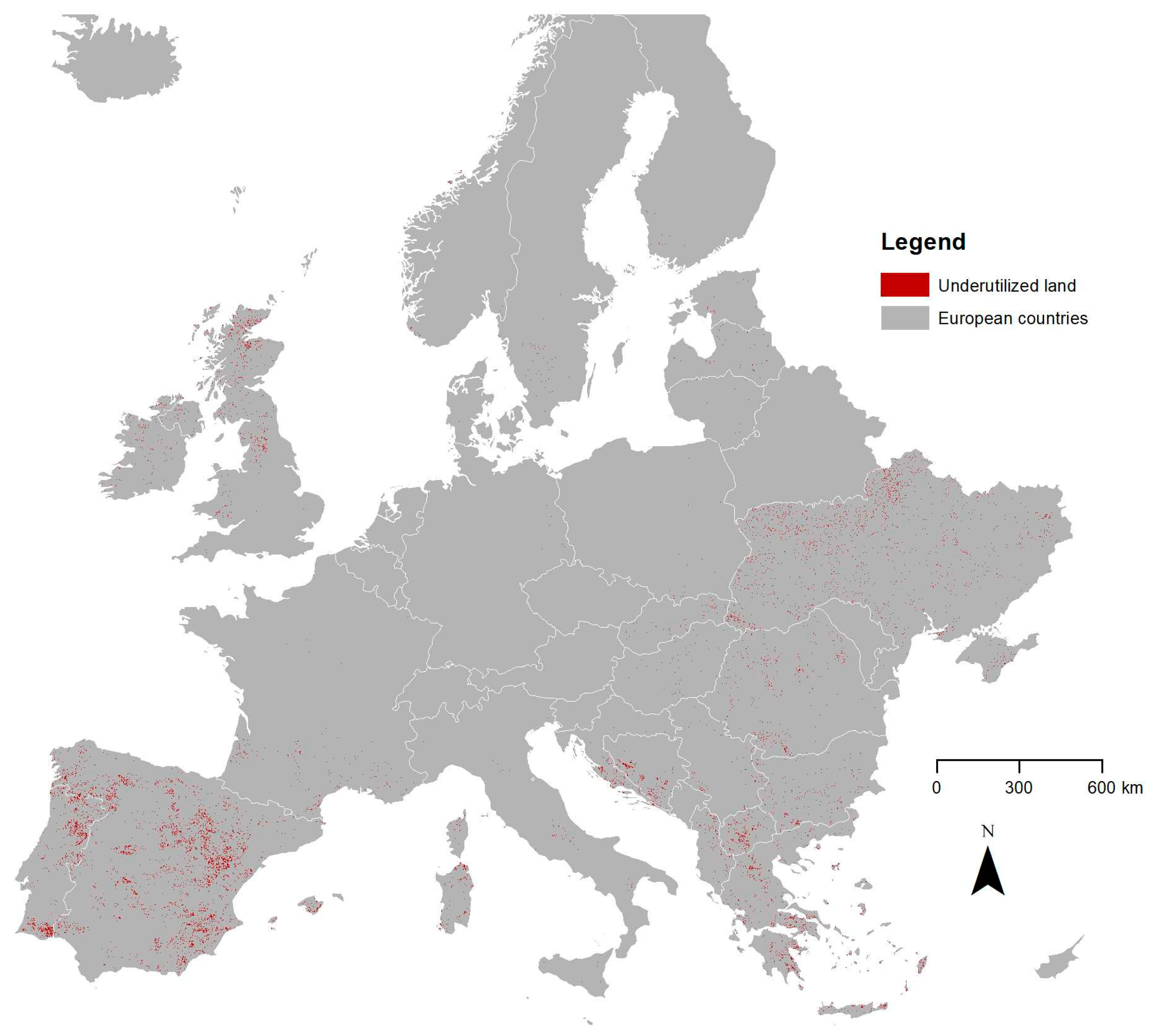
In the accuracy assessment, we discarded all points flagged as “not reliable”. The points flagged as “borders” and “small stripes” were considered correct in both cases. In the case of “borders”, the geometric accuracy was not high enough in Google Earth to be sure to assign a class. In the case of small stripes, the geometric resolution of the Landsat data would not allow a differentiation.

4. Results

The classification yielded a total of 5.3 million ha of UU land, which corresponds to 2.44% of the area of interest. The results per biogeographical region are given in

Table 4. Area-based accuracy measures of the classification per biogeographical region and overall.

Biogeographical Region	OA (%) (CI)	U: OE (%) (CI)	U: CE (%) (CI)	UU: OE (%) (CI)	UU: CE (%) (CI)
Alpine	62.16 (8.82)	1.17 (0.65)	37.84 (9.06)	95.55 (1.12)	38.00 (13.59)
Atlantic	91.43 (2.31)	0.37 (0.12)	8.42 (2.33)	92.24 (2.24)	32.43 (10.57)
Boreal	90.62 (3.61)	0.06 (0.03)	9.69 (3.62)	98.38 (0.63)	24.00 (11.96)
Continental	90.62 (2.10)	0.52 (0.13)	9.06 (2.14)	88.08 (2.65)	27.74 (7.07)
Mediterranean	70.08 (5.19)	1.74 (0.50)	31.30 (5.63)	80.75 (2.87)	14.00 (3.93)
Pannonian	98.17 (2.88)	0.40 (0.21)	1.49 (2.93)	51.61 (48.78)	22.00 (11.60)
Steppic	85.28 (4.96)	0.32 (0.14)	14.58 (5.01)	95.77 (1.53)	30.00 (12.83)
Overall	85.52 (1.55)	0.66 (1.55)	14.27 (1.50)	88.06 (1.32)	22.77 (3.05)

, and the resulting map is shown in Figure 6. The total area of UU land per biogeographical regions is by far highest in the Mediterranean region followed by the Continental region. This is not surprising, as these two regions are also the overall largest biogeographical regions in Europe. However, we want to reiterate that the area of interest comprised only areas outside the elimination mask of steep slopes, wetlands, settlements, etc. (see Section 3). This area of interest per biogeographic region is also given in Table 2 and it was much smaller for the Mediterranean than for the Continental region. Calculating the UU land in relation to this area, the Mediterranean region showed the highest share of UU land with almost 8% followed by the Alpine region with 2.76%. The Continental region, in contrast, shows only 1.66% UU land of the area of interest. The smallest share of UU land was found in the Boreal region. In terms of countries, the largest amounts were found in Spain, Ukraine, Greece, North-Macedonia, Portugal, Croatia, Bosnia–Herzegovina, and Bulgaria, but also in Italy and Great Britain. Very little underutilized land was found in the Scandinavian countries, in Germany, Austria, and the Benelux countries (Figure 6).

We further analyzed the identified UU land patches regarding average size and compactness. The largest average patches, with almost 50 ha per UU land patch, were found in the Mediterranean region, followed by 39.2 ha in the Alpine and 33.7 ha in the Atlantic region. The smallest patch sizes were found in the Steppic region, with 23.2 ha on average. In order to assess the compactness, we calculated index i as the relation of the polygon’s area to the area of a theoretical circle with the same perimeter as the polygon. The index was calculated as given in Equation (1) below:

$$i=\frac{A_p*4\pi }{P_{p}2}$$

(1)

where

i is the compactness index;

A_p is the area of the polygon; and

P_p is the perimeter of the polygon.

The higher the index, the more compact the patches are; an i = 1 would be a fully compact circle. Generally, the compactness values are quite low, but differences can still be observed. While UU land in the boreal region appeared relatively compact (0.28), the lowest compactness values were observed in the Mediterranean and in the Continental regions (both approx. 0.19).

For the validation of the map, a total of 2605 blindly interpreted points were finally used. The distribution to the classes and sub-classes is given in Table 3 according to the method described above. For the calculation of the accuracy figures, the weights per point were adapted according to the area of the respective sub-class [50].

The resulting accuracy values, overall accuracy (OA), omission error (OE), and commission error (CE) for each biogeographical region are given in Table 4. Due to the application of the resulting map as an input for stakeholder involvement, we considered the CE of UU land more critical than OE of UU land. CE relates to lands that are classified as underutilized but in reality are utilized. This would be a much more problematic error from the potential users’ perspective than omitting certain UU lands (OE). The quality of the results is therefore considered mainly based on the OA and CE of UU land. With respect to the biogeographical regions, the best results in OA were achieved for the Pannonian region followed by the Atlantic region. Based on the total areas of UU land, being largest in the Mediterranean and the Continental regions, they should be assessed in more detail. Although the OA for the Mediterranean region was lower than for the other regions (70%), both the CE of UU land (14%) and a CI of only 3.9% at 95% CL were good. The reason for the lower OA in the Mediterranean region was mostly due to the similarity of phenological profiles of permanent crops and underutilized lands. Although we eliminated permanent cropland using CLC, given the fact that the CLC had an MMU of 25 ha, all permanent croplands smaller than 25 ha but larger than 10 ha remained in the area of interest of our assessment, leading to OE and CE. For the Continental region, the OA was above 90% with a small CI (2.1%) but with higher CE (27.74 ± 7%). The most critical region was the Alpine region with the lowest OA of only 62%, a high CI (8.8%), and also the highest CE for UU land (38%). The reasons can be found in the very small-structured landscape and strong topography, on the one hand, and in the comparably higher cloud coverage hampering both the classification and the validation, on the other hand. Many validation points in this region had to be discarded due to missing or not interpretable data leading to higher weights being assigned to the remaining points. Generally, many reasons can be mentioned for the differences between regions: different properties of UU land, which we might not have covered despite our efforts to be representative; similarities of UU land with specific used land categories (low-intensity grazing in the Alpine or Mediterranean regions for example); or limited satellite data availability in specific regions (e.g., frequent cloud cover at western mountain sides), impeding the generation of meaningful time series statistics.

In comparison to existing studies, this is the first work to our knowledge that employs HR time series data for continental-wide mapping of underutilized land. Previously presented methods based on MODIS would not be able to detect the relatively small patches, often characterized by low compactness, which are typical in many parts of Europe. The average size of the UU land patches varies between 23.2 and 49.6 ha (see Table 2). Using MODIS data with a geometric resolution of 500 × 500 m (25 ha for one pixel!), it would not be possible to identify most of these patches. The low compactness values would further deteriorate the quality of a MODIS-based assessment due to large shares of mixed pixels in the UU land patches. In [12], a map of abandoned farmland for 2010 with a resolution of 300 × 300 m for former Soviet Union countries was generated using multiple existing global and regional data sources. This map of Ukraine shows more than 5 million ha abandoned agricultural farmland with a mean patch size of 35.8 ha [12]. We identified with 820,400 ha considerably fewer areas and also smaller patches (mean patch size 26.8 ha). Figure 7 shows a comparison of both data sets for a small part of Ukraine, highlighting the similarities and differences in patch structures. There are several reasons for both the difference in total area and in patch size. The first reason is the different date of assessment: 2010 [12] versus 2015–2019. It may well be that parts of the land have been used again after being idle for some years in the beginning of the century. The second and probably more significant reason is the already discussed consideration of young, regenerating forest on previously agricultural lands, which were considered in [12] but not considered in our study. The third reason can be found in the source data used, which are completely different. While our approach relied on Landsat and S2 data over 5 years, in [12], the authors took into account several different existing global and regional data sources. Finally, our processing excluded steep slopes and wetlands, which are typically the first areas to be abandoned because of higher efforts in agricultural treatments. Due to these temporal and methodical differences, the two maps could not be compared directly.

It could be shown that it is possible to generate a continental map of underutilized land from time series analysis of L8 and S2 data with reasonable accuracy. Existing Copernicus thematic maps have been used for both training and for elimination of unsuitable areas. The resulting data are in line with previous findings [47] showing larger areas of underutilized lands in the Mediterranean and especially in the eastern parts of the Continental region than in other regions.

However, there is also a strong difference between countries. While for Ukraine we identified almost 820,400 ha, there were not even 5000 ha of UU land identified for Germany, although both countries largely belong to the continental region. Clearly, the reason can be found in the different agricultural structures and traditions in these two countries, as supported by [47].

In conclusion, the current work delivers a valuable data base and overview of existing underutilized lands on a continental scale with some limitations with regards to small structured agricultural patches. In order to improve the quality to a sub-national scale, future research should investigate the use of a complete S2 time series for 2017–2020, making full use of the higher spatial and temporal resolution of S2 compared to L8. Additional improvements should include the use of the full time series model, as was done for other applications [48], rather than the limitations on certain temporal features, as was employed in this study. Within the BIOPLAT-EU project, several case study areas were identified and will be mapped in more detail, giving better insight in local situations and applicability.

5. Conclusions

This study demonstrated the use of high resolution Landsat 8 and Sentinel-2 time series data for the classification of underutilized land on a continental scale and a considerable level of detail. The cloud processing platform Google Earth Engine proved to be a valuable tool for efficient processing when large amounts of satellite data are to be included in an continental image classification The results of this study do not only provide valuable information on the European-wide availability of underutilized lands potentially usable for bioenergy feedstock production but also deliver insight into their geographical distribution. The overall accuracies achieved are generally very good (OA = 85.5%), leading to a potential of underutilized land for bioenergy of 5.3 million ha (between 4.1 and 10 million ha at 95% CL). Regarding the geographical distribution, it turned out that the highest potentials for bioenergy feedstock production can be found in the Mediterranean and in the eastern part of the Continental region, the latter largely due to the integration of the Ukraine territory into the analysis.

Though having information on the amount and location of underutilized lands potentially available for bioenergy feedstock production, it is difficult to estimate how much the feedstock production on these lands can contribute to achieving the aim of the REDII directive (32% energy production from renewable sources). There are always other social and (mainly) economic barriers that do not allow the production/investments to be profitable and therefore feasible on the identified lands. Lack of policies and infrastructures are also barriers to the feasibility. In addition, there are proponents of keeping such lands untouched, e.g., for nature conservation. Further assessments using advanced models (e.g., STEN) that connect the underutilized land patches with additional influencing factors are needed to be able to assess the final contribution.

References

1. European Commission. Directive (EU) 2018/2001 of the European Parliament and of the Council of 11 December 2018 on the Promotion of the Use of Energy from Renewable Sources. Official Journal of the European Union, L328/82. Available online: https://eur-lex.europa.eu/legal-content/EN/TXT/PDF/?uri=CELEX:32018L2001 (accessed on 21 January 2021).
2. Longato, D.; Gaglio, M.; Boschetti, M.; Gissi, E. Bioenergy and Ecosystem Services Trade-Offs and Synergies in Marginal Agricultural Lands: A Remote-Sensing-Based Assessment Method. J. Clean. Prod. 2019, 237, 117672. [Google Scholar] [CrossRef]
3. Smeets, E.; Faaij, A.; Lewandowski, I.; Turkenburg, W. A Bottom-up Assessment and Review of Global Bio-Energy Potentials to 2050. Prog. Energy Combust. Sci. 2007, 33, 56–106. [Google Scholar] [CrossRef] [Green Version]
4. Nijsen, M.; Smeets, E.; Stehfest, E.; Vuuren, D.P. An Evaluation of the Global Potential of Bioenergy Production on Degraded Lands. GCB Bioenergy 2012, 4, 130–147. [Google Scholar] [CrossRef]
5. Robledo-Abad, C.; Althaus, H.-J.; Berndes, G.; Bolwig, S.; Corbera, E.; Creutzig, F.; Garcia-Ulloa, J.; Geddes, A.; Gregg, J.S.; Haberl, H.; et al. Bioenergy Production and Sustainable Development: Science Base for Policymaking Remains Limited. GCB Bioenergy 2017, 9, 541–556. [Google Scholar] [CrossRef] [PubMed] [Green Version]
6. Humpenöder, F.; Popp, A.; Bodirsky, B.L.; Weindl, I.; Biewald, A.; Lotze-Campen, H.; Dietrich, J.P.; Klein, D.; Kreidenweis, U.; Müller, C.; et al. Large-Scale Bioenergy Production: How to Resolve Sustainability Trade-Offs? Environ. Res. Lett. 2018, 13, 024011. [Google Scholar] [CrossRef] [Green Version]
7. Alcantara, C.; Kuemmerle, T.; Baumann, M.; Bragina, E.V.; Griffiths, P.; Hostert, P.; Knorn, J.; Müller, D.; Prishchepov, A.V.; Schierhorn, F.; et al. Mapping the Extent of Abandoned Farmland in Central and Eastern Europe Using MODIS Time Series Satellite Data. Environ. Res. Lett. 2013, 8, 035035. [Google Scholar] [CrossRef]
8. Estel, S.; Kuemmerle, T.; Alcántara, C.; Levers, C.; Prishchepov, A.; Hostert, P. Mapping Farmland Abandonment and Recultivation across Europe Using MODIS NDVI Time Series. Remote Sens. Environ. 2015, 163, 312–325. [Google Scholar] [CrossRef]
9. Estel, S. Mapping Cropland-Use Intensity across Europe Using MODIS NDVI Time Series. Environ. Res. Lett. 2016, 11, 024015. [Google Scholar] [CrossRef] [Green Version]
10. Feranec, J.; Soukup, T.; Taff, G.; Stych, P.; Bičík, I. Overview of Changes in Land Use and Land Cover in Eastern Europe. In Land-Cover and Land-Use Changes in Eastern Europe after the Collapse of the Soviet Union in 1991; Springer: Cham, Switzerland, 2017; pp. 13–33. [Google Scholar]
11. Löw, F.; Prishchepov, A.; Waldner, F.; Dubovyk, O.; Akramkhanov, A.; Biradar, C.; Lamers, J. Mapping Cropland Abandonment in the Aral Sea Basin with MODIS Time Series. Remote Sens. 2018, 10, 159. [Google Scholar] [CrossRef] [Green Version]
12. Lesiv, M.; Schepaschenko, D.; Moltchanova, E.; Bun, R.; Dürauer, M.; Prishchepov, A.V.; Schierhorn, F.; Estel, S.; Kuemmerle, T.; Alcántara, C.; et al. Spatial Distribution of Arable and Abandoned Land across Former Soviet Union Countries. Sci. Data 2018, 5. [Google Scholar] [CrossRef]
13. Lieskovský, J.; Bezák, P.; Špulerová, J.; Lieskovský, T.; Koleda, P.; Dobrovodská, M.; Bürgi, M.; Gimmi, U. The Abandonment of Traditional Agricultural Landscape in Slovakia—Analysis of Extent and Driving Forces. J. Rural Stud. 2015, 37, 75–84. [Google Scholar] [CrossRef]
14. Szatmári, D.; Kopecka, M.; Feranec, J.; Goga, T. Abandoned Agricultural Land Mapping Using Sentinel-2a Data. In Proceedings of the 7th International Conference on Cartography and GIS, Sozopol, Bulgaria, 18–23 June 2018; Bandrova, T., Konečný, M., Eds.; 2018. Available online: https://www.researchgate.net/publication/325644850_ABANDONED_AGRICULTURAL_LAND_MAPPING_USING_SENTINEL-2A_DATA (accessed on 21 January 2021).
15. Baumann, M.; Kuemmerle, T.; Elbakidze, M.; Ozdogan, M.; Radeloff, V.C.; Keuler, N.S.; Prishchepov, A.V.; Kruhlov, I.; Hostert, P. Patterns and Drivers of Post-Socialist Farmland Abandonment in Western Ukraine. Land Use Policy 2011, 28, 552–562. [Google Scholar] [CrossRef]
16. Gorelick, N.; Hancher, M.; Dixon, M.; Ilyushchenko, S.; Thau, D.; Moore, R. Google Earth Engine: Planetary-Scale Geospatial Analysis for Everyone. Remote Sens. Environ. 2017, 202, 18–27. [Google Scholar] [CrossRef]
17. ETC/BD. The Indicative Map of European Biogeographical Regions: Methodology and Development. 2006. Available online: https://www.google.at/url?sa=t&rct=j&q=&esrc=s&source=web&cd=&ved=2ahUKEwiS5b7b_azuAhWL-KQKHd8CAv4QFjABegQIAhAC&url=https%3A%2F%2Fwww.eea.europa.eu%2Fdata-and-maps%2Fdata%2Fbiogeographical-regions-europe-2005%2Fmethodology-description-pdf-format%2Fmethodology-description-pdf-format%2Fdownload&usg=AOvVaw1sSWT_9h8yBy36ULNiBgjI (accessed on 21 January 2021).
18. European Environmental Agency (EEA). Biogeographical Regions. Available online: https://www.eea.europa.eu/data-and-maps/data/biogeographical-regions-europe-3#tab-metadata (accessed on 16 December 2020).
19. Joshi, N.; Baumann, M.; Ehammer, A.; Fensholt, R.; Grogan, K.; Hostert, P.; Jepsen, M.; Kuemmerle, T.; Meyfroidt, P.; Mitchard, E.; et al. A Review of the Application of Optical and Radar Remote Sensing Data Fusion to Land Use Mapping and Monitoring. Remote Sens. 2016, 8, 70. [Google Scholar] [CrossRef] [Green Version]
20. Roy, D.P.; Wulder, M.A.; Loveland, T.R.; Woodcock, C.; Allen, R.G.; Anderson, M.C.; Helder, D.; Irons, J.R.; Johnson, D.M.; Kennedy, R.; et al. Landsat-8: Science and Product Vision for Terrestrial Global Change Research. Remote Sens. Environ. 2014, 145, 154–172. [Google Scholar] [CrossRef] [Green Version]
21. U.S. Geological Survey. Landsat 8 Collection 1 (C1) Land Surface Reflectance Code (LaSRC) Product Guide 2020. Available online: https://www.usgs.gov/media/files/landsat-8-collection-1-land-surface-reflectance-code-product-guide (accessed on 21 January 2021).
22. Wulder, M.A.; Masek, J.G.; Cohen, W.B.; Loveland, T.R.; Woodcock, C.E. Opening the Archive: How Free Data Has Enabled the Science and Monitoring Promise of Landsat. Remote Sens. Environ. 2012, 122, 2–10. [Google Scholar] [CrossRef]
23. Aschbacher, J.; Milagro-Pérez, M.P. The European Earth Monitoring (GMES) Programme: Status and Perspectives. Remote Sens. Environ. 2012, 120, 3–8. [Google Scholar] [CrossRef]
24. Drusch, M.; Del Bello, U.; Carlier, S.; Colin, O.; Fernandez, V.; Gascon, F.; Hoersch, B.; Isola, C.; Laberinti, P.; Martimort, P.; et al. Sentinel-2: ESA’s Optical High-Resolution Mission for GMES Operational Services. Remote Sens. Environ. 2012, 120, 25–36. [Google Scholar] [CrossRef]
25. Friedl, P. Derivation of Glaciological Parameters from Time Series of Multi-Mission Remote Sensing Data—Applications to Glaciers in Antarctica and the Karakoram. Ph.D. Thesis, Friedrich-Alexander-University of Erlangen-Nürnberg, Erlangen, Germany, 2020. [Google Scholar]
26. Houghton, R.A.; Nassikas, A.A. Global and Regional Fluxes of Carbon from Land Use and Land Cover Change 1850–2015. Glob. Biogeochem. Cycles 2017, 31, 456–472. [Google Scholar] [CrossRef]
27. Kuemmerle, T.; Olofsson, P.; Chaskovskyy, O.; Baumann, M.; Ostapowicz, K.; Woodcock, C.E.; Houghton, R.A.; Hostert, P.; Keeton, W.S.; Radeloff, V.C. Post-Soviet Farmland Abandonment, Forest Recovery, and Carbon Sequestration in Western Ukraine: Carbon Sequestration on Abandoned Farmland. Glob. Chang. Biol. 2011, 17, 1335–1349. [Google Scholar] [CrossRef]
28. Lesiv, M.; Shvidenko, A.; Schepaschenko, D.; See, L.; Fritz, S. A Spatial Assessment of the Forest Carbon Budget for Ukraine. Mitig. Adapt. Strateg. Glob. Chang. 2019, 24, 985–1006. [Google Scholar] [CrossRef] [Green Version]
29. Smaliychuk, A.; Müller, D.; Prishchepov, A.V.; Levers, C.; Kruhlov, I.; Kuemmerle, T. Recultivation of Abandoned Agricultural Lands in Ukraine: Patterns and Drivers. Glob. Environ. Chang. 2016, 38, 70–81. [Google Scholar] [CrossRef]
30. Rhemtulla, J.M.; Mladenoff, D.J.; Clayton, M.K. Historical Forest Baselines Reveal Potential for Continued Carbon Sequestration. Proc. Natl. Acad. Sci. USA 2009, 106, 6082–6087. [Google Scholar] [CrossRef] [PubMed] [Green Version]
31. Russi, D.; ten Brink, P.; Farmer, A.; Badura, T.; Coates, D.; Förster, J.; Kumar, R.; Davidson, N. The Economics of Ecosystems and Biodiversity for Water and Wetlands. IEEP Lond. Bruss. 2013, 78. Available online: https://www.cbd.int/financial/values/g-ecowaterwetlands-teeb.pdf (accessed on 21 January 2021).
32. Myroniuk, V.; Kutia, M.; Sarkissian, A.J.; Bilous, A.; Liu, S. Regional-Scale Forest Mapping over Fragmented Landscapes Using Global Forest Products and Landsat Time Series Classification. Remote Sens. 2020, 12, 187. [Google Scholar] [CrossRef] [Green Version]
33. Foga, S.; Scaramuzza, P.L.; Guo, S.; Zhu, Z.; Dilley, R.D.; Beckmann, T.; Schmidt, G.L.; Dwyer, J.L.; Joseph Hughes, M.; Laue, B. Cloud Detection Algorithm Comparison and Validation for Operational Landsat Data Products. Remote Sens. Environ. 2017, 194, 379–390. [Google Scholar] [CrossRef] [Green Version]
34. Wu, C.; Niu, Z.; Tang, Q.; Huang, W. Estimating Chlorophyll Content from Hyperspectral Vegetation Indices: Modeling and Validation. Agric. For. Meteorol. 2008, 148, 1230–1241. [Google Scholar] [CrossRef]
35. Clevers, J.G.P.W.; Gitelson, A.A. Remote Estimation of Crop and Grass Chlorophyll and Nitrogen Content Using Red-Edge Bands on Sentinel-2 and -3. Int. J. Appl. Earth Obs. Geoinf. 2013, 23, 344–351. [Google Scholar] [CrossRef]
36. Sonobe, R.; Yamaya, Y.; Tani, H.; Wang, X.; Kobayashi, N.; Mochizuki, K. Crop Classification from Sentinel-2-Derived Vegetation Indices Using Ensemble Learning. J. Appl. Remote Sens. 2018, 12, 1. [Google Scholar] [CrossRef] [Green Version]
37. Sharifi, A. Remotely Sensed Vegetation Indices for Crop Nutrition Mapping. J. Sci. Food Agric. 2020, 100, 5191–5196. [Google Scholar] [CrossRef]
38. Mercier, A.; Betbeder, J.; Baudry, J.; Le Roux, V.; Spicher, F.; Lacoux, J.; Roger, D.; Hubert-Moy, L. Evaluation of Sentinel-1 & 2 Time Series for Predicting Wheat and Rapeseed Phenological Stages. ISPRS J. Photogramm. Remote Sens. 2020, 163, 231–256. [Google Scholar]
39. Daughtry, C.S.T.; Walthall, C.L.; Kim, M.S.; de Colstoun, E.B.; McMurtrey, J.E. Estimating Corn Leaf Chlorophyll Concentration from Leaf and Canopy Reflectance. Remote Sens. Environ. 2000, 74, 229–239. [Google Scholar] [CrossRef]
40. Kim, M.S. The Use of Narrow Spectral Bands for Improving Remote Sensing Estimation of Fractionally Absorbed Photosynthetically Active Radiation (FAPAR). Master’s Thesis, Department of Geography, University of Maryland, College Park, MD, USA, 1994. [Google Scholar]
41. Qi, J.; Chehbouni, A.; Huete, A.R.; Kerr, Y.H.; Sorooshian, S. A Modified Soil Adjusted Vegetation Index. Remote Sens. Environ. 1994, 48, 119–126. [Google Scholar] [CrossRef]
42. Liaw, A.; Wiener, M. Classification and Regression by RandomForest. R News 2002, 2, 18–22. [Google Scholar]
43. Horning, N. Random Forests: An Algorithm for Image Classification and Generation of Continuous Fields Data Sets. In Proceedings of the International Conference on Geoinformatics for Spatial Infrastructure Development in Earth and Allied Sciences, Osaka, Japan, 9–11 December 2010. [Google Scholar]
44. Li, T.; Ni, B.; Wu, X.; Gao, Q.; Li, Q.; Sun, D. On Random Hyper-Class Random Forest for Visual Classification. Neurocomputing 2016, 172, 281–289. [Google Scholar] [CrossRef]
45. Ali, J.; Khan, R.; Ahmad, N.; Maqsood, I. Random Forests and Decision Trees. Int. J. Comput. Sci. Issues IJCSI 2012, 9, 272. [Google Scholar]
46. Grinand, C.; Rakotomalala, F.; Gond, V.; Vaudry, R.; Bernoux, M.; Vieilledent, G. Estimating Deforestation in Tropical Humid and Dry Forests in Madagascar from 2000 to 2010 Using Multi-Date Landsat Satellite Images and the Random Forests Classifier. Remote Sens. Environ. 2013, 139, 68–80. [Google Scholar] [CrossRef]
47. Gómez, C.; White, J.C.; Wulder, M.A. Optical Remotely Sensed Time Series Data for Land Cover Classification: A Review. ISPRS J. Photogramm. Remote Sens. 2016, 116, 55–72. [Google Scholar] [CrossRef] [Green Version]
48. Dalponte, M.; Ørka, H.O.; Gobakken, T.; Gianelle, D.; Næsset, E. Tree Species Classification in Boreal Forests with Hyperspectral Data. IEEE Trans. Geosci. Remote Sens. 2012, 51, 2632–2645. [Google Scholar] [CrossRef]
49. Mellor, A.; Boukir, S.; Haywood, A.; Jones, S. Exploring Issues of Training Data Imbalance and Mislabelling on Random Forest Performance for Large Area Land Cover Classification Using the Ensemble Margin. ISPRS J. Photogramm. Remote Sens. 2015, 105, 155–168. [Google Scholar] [CrossRef]
50. Olofsson, P.; Foody, G.M.; Herold, M.; Stehman, S.V.; Woodcock, C.E.; Wulder, M.A. Good Practices for Estimating Area and Assessing Accuracy of Land Change. Remote Sens. Environ. 2014, 148, 42–57. [Google Scholar] [CrossRef]
Figure 1. Study area and stratification for processing.
Land 10 00102 g001
Figure 2. L8 NDVI phenological profiles of underutilized lands in different biogeographical regions.
Land 10 00102 g002
Figure 3. Spectral resolution of currently available optical satellite sensors grouped by different domains of the electromagnetic spectrum (VIS = visible, NIR = near infrared, VNIR = visible near infrared, SWIR = shortwave infrared, TIR = thermal infrared) [25].
Land 10 00102 g003
Figure 4. Workflow diagram of the applied mapping approach.
Land 10 00102 g004
Figure 5. L8 NDVI phenological profiles of cropland (orange), managed grassland (green), and underutilized land (blue) in the Continental biogeographical region. The growing season (beginning of May until end of September) is indicated in grey.
Land 10 00102 g005
Figure 6. Final map of underutilized land in Europe.
Land 10 00102 g006
Figure 7. Comparison of the map of abandoned agricultural farmland produced by [12] for 2010 and the results of this study.
Land 10 00102 g007