Spatial Variations of Vegetation Index from Remote Sensing Linked to Soil Colloidal Status


Abstract
1. Introduction
2. Methods
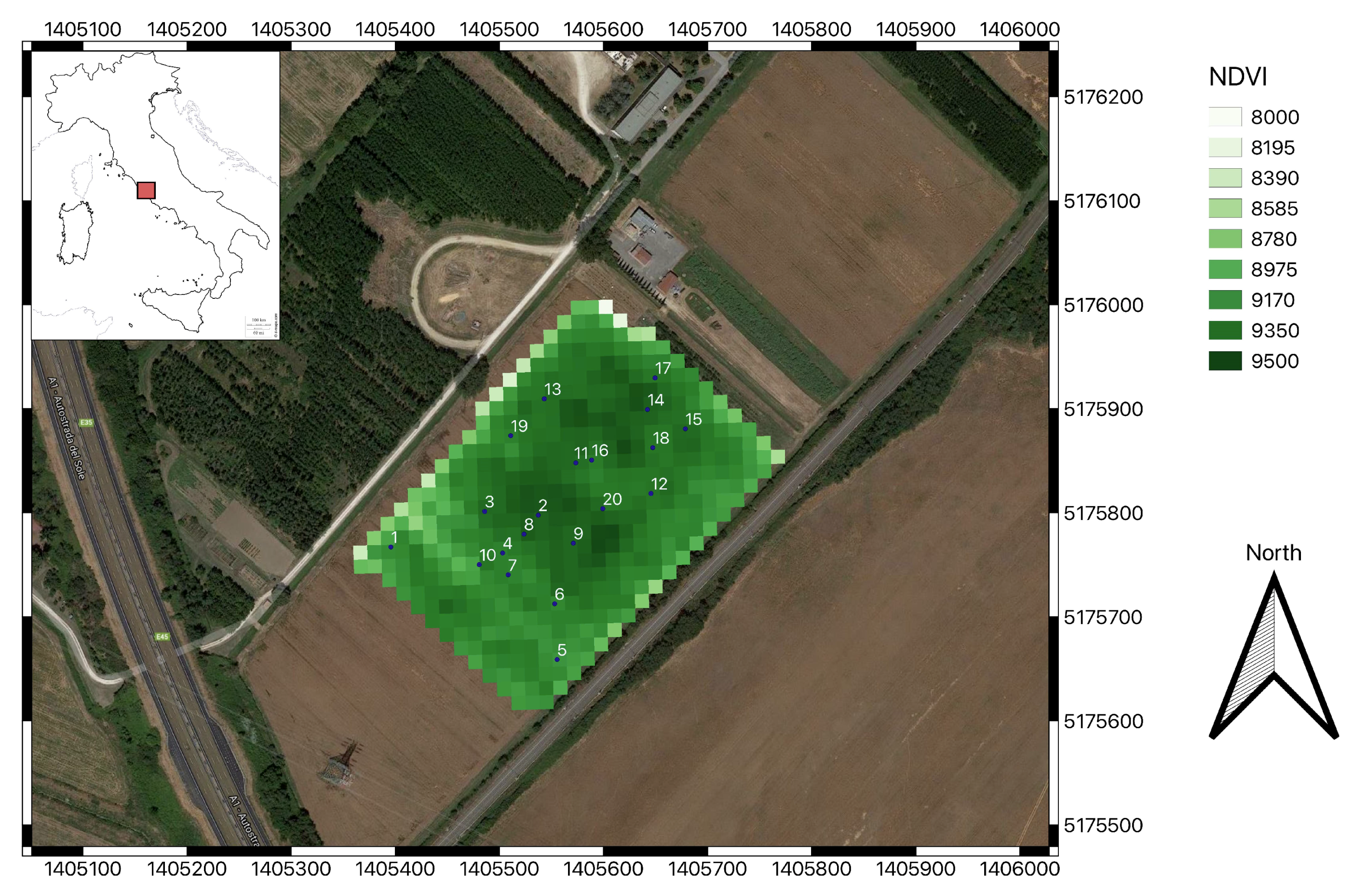
2.1. Study Site
2.2. Vegetation Model
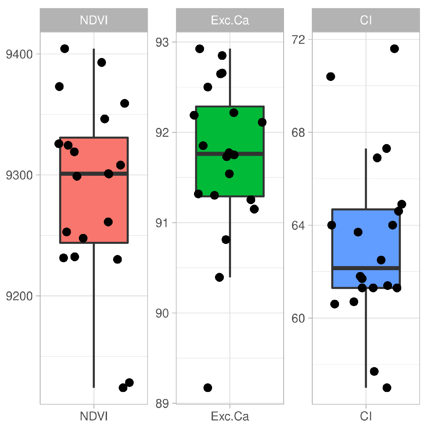
- an exponential function for CI (where denotes the variance function evaluated at CI and t is the variance function coefficient, t = −0.39);
- a power function for exchangeable Ca (t = −0.32).
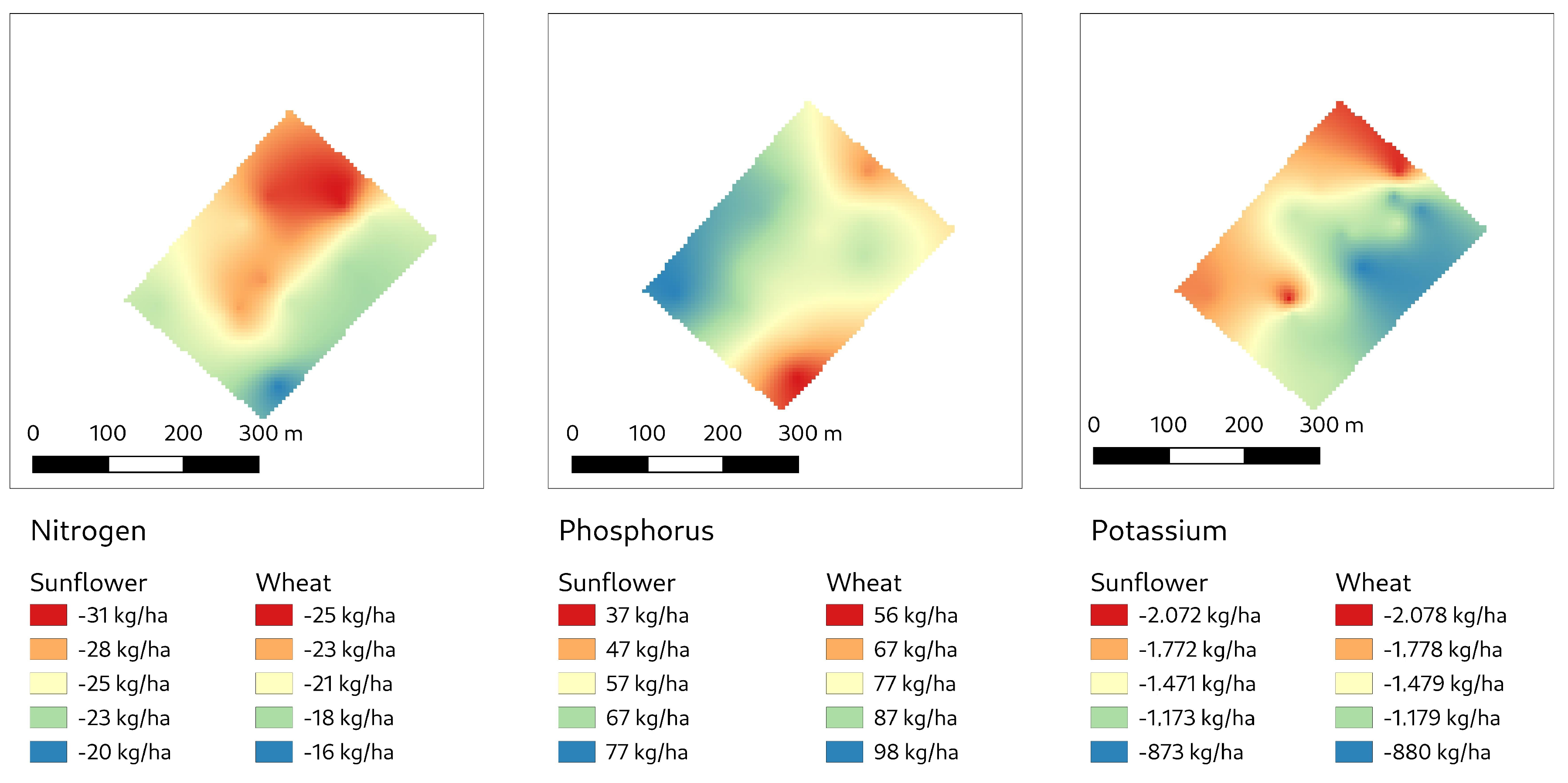
2.3. Fertilization Plans
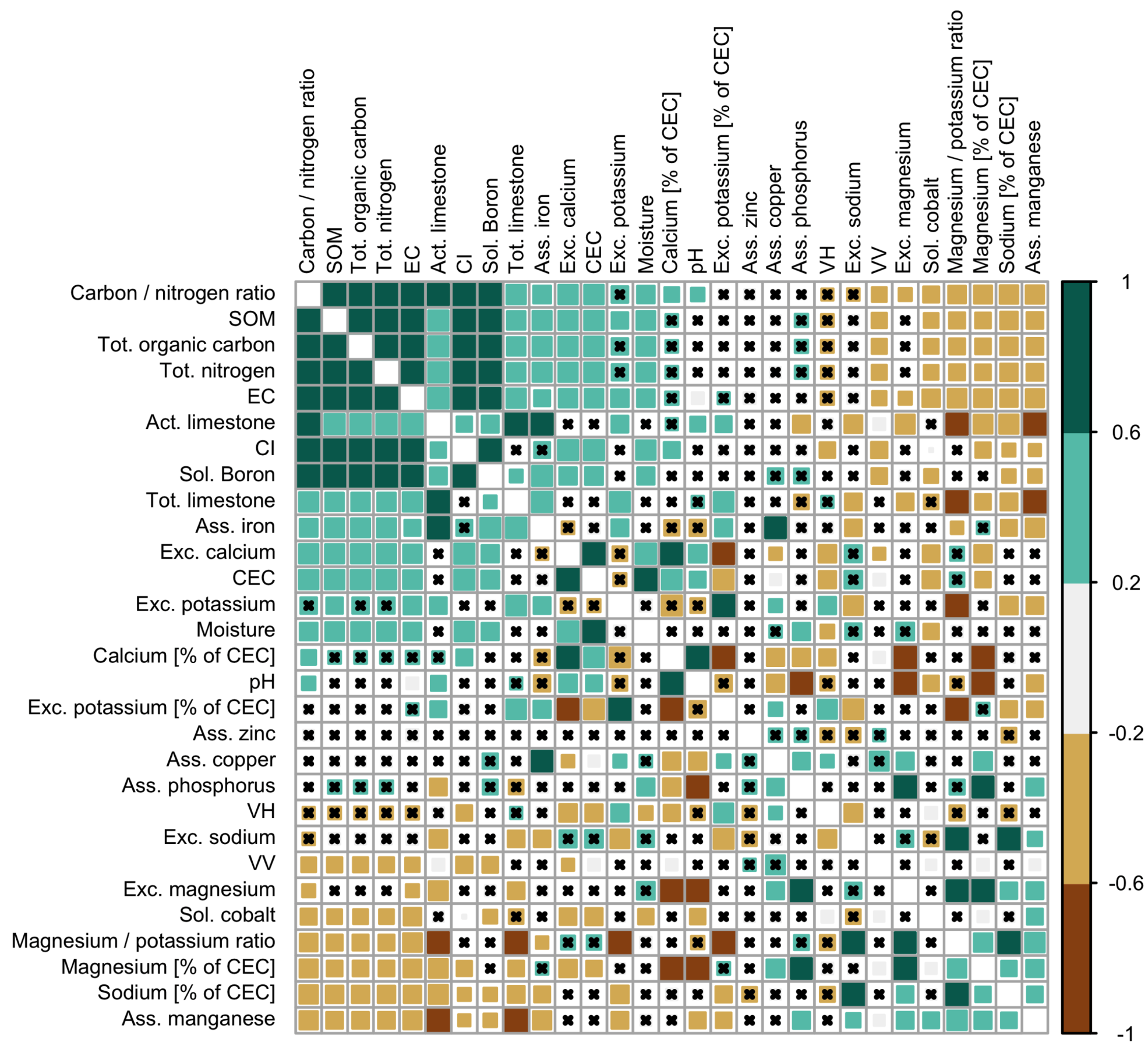
3. Results
4. Discussion
5. Conclusions
Author Contributions
Funding
Institutional Review Board Statement
Informed Consent Statement
Data Availability Statement
Conflicts of Interest
References
- Schlesinger, W. An overview of the C cycle. In Soils and Global Change; Lal, R., Kimble, J., Levin, J., Stewart, B.A., Eds.; CRC: Boca Raton, FL, USA, 1995; pp. 9–26. [Google Scholar]
- Paul, E.A. The nature and dynamics of soil organic matter: Plant inputs, microbial transformations, and organic matter stabilization. Soil Biol. Biochem. 2016, 98, 109–126. [Google Scholar] [CrossRef]
- Gomiero, T. Soil Degradation, Land Scarcity and Food Security: Reviewing a Complex Challenge. Sustainability 2016, 8, 281. [Google Scholar] [CrossRef]
- Branca, G.; Lipper, L.; McCarthy, N.; Jolejole, M.C. Food security, climate change, and sustainable land management. A review. Agron. Sustain. Dev. 2013, 33, 635–650. [Google Scholar] [CrossRef]
- Ritsema, C.J.; Lynden, G.W.J.V.; Jetten, V.G.; Jong, S.M.D. DEGRADATION. In Encyclopedia of Soils in the Environment; Hillel, D., Ed.; Elsevier: Oxford, UK, 2005; pp. 370–377. [Google Scholar] [CrossRef]
- Pereira, P.; Brevik, E.C.; Oliva, M.; Estebaranz, F.; Depellegrin, D.; Novara, A.; Cerdà, A.; Menshov, O. Chapter 3—Goal Oriented Soil Mapping: Applying Modern Methods Supported by Local Knowledge. In Soil Mapping and Process Modeling for Sustainable Land Use Management; Pereira, P., Brevik, E.C., Muñoz-Rojas, M., Miller, B.A., Eds.; Elsevier: Oxford, UK, 2017; pp. 61–83. [Google Scholar] [CrossRef]
- Purwanto, B.H.; Alam, S. Impact of intensive agricultural management on carbon and nitrogen dynamics in the humid tropics. Soil Sci. Plant Nutr. 2020, 66, 50–59. [Google Scholar] [CrossRef]
- Vizzari, M.; Santaga, F.; Benincasa, P. Sentinel 2-Based Nitrogen VRT Fertilization in Wheat: Comparison between Traditional and Simple Precision Practices. Agronomy 2019, 9, 278. [Google Scholar] [CrossRef]
- Song, Y.Q.; Zhao, X.; Su, H.Y.; Li, B.; Hu, Y.M.; Cui, X.S. Predicting Spatial Variations in Soil Nutrients with Hyperspectral Remote Sensing at Regional Scale. Sensors 2018, 18, 3086. [Google Scholar] [CrossRef]
- Khitrov, N.B.; Rukhovich, D.I.; Koroleva, P.V.; Kalinina, N.V.; Trubnikov, A.V.; Petukhov, D.A.; Kulyanitsa, A.L. A study of the responsiveness of crops to fertilizers by zones of stable intra-field heterogeneity based on big satellite data analysis. Arch. Agron. Soil Sci. 2020, 66, 1963–1975. [Google Scholar] [CrossRef]
- Tewes, A.; Hoffmann, H.; Nolte, M.; Krauss, G.; Schäfer, F.; Kerkhoff, C.; Gaiser, T. How Do Methods Assimilating Sentinel-2-Derived LAI Combined with Two Different Sources of Soil Input Data Affect the Crop Model-Based Estimation of Wheat Biomass at Sub-Field Level? Remote Sens. 2020, 12, 925. [Google Scholar] [CrossRef]
- Hongo, C.; Sigit, G.; Shikata, R.; Niwa, K.; Tamura, E. The Use of Remotely Sensed Data for Estimating of Rice Yield Considering Soil Characteristics. J. Agric. Sci. 2014, 6, 13. [Google Scholar]
- Bascietto, M.; Sperandio, G.; Bajocco, S. Efficient Estimation of Biomass from Residual Agroforestry. ISPRS Int. J. Geo-Inf. 2020, 9, 21. [Google Scholar] [CrossRef]
- Mulla, D.J. Twenty five years of remote sensing in precision agriculture: Key advances and remaining knowledge gaps. Biosyst. Eng. 2013, 114, 358–371. [Google Scholar] [CrossRef]
- Weiss, M.; Jacob, F.; Duveiller, G. Remote sensing for agricultural applications: A meta-review. Remote Sens. Environ. 2020, 236, 111402. [Google Scholar] [CrossRef]
- Auernhammer, H. Precision farming—The environmental challenge. Comput. Electron. Agric. 2001, 30, 31–43. [Google Scholar] [CrossRef]
- Basso, B.; Fiorentino, C.; Cammarano, D.; Schulthess, U. Variable rate nitrogen fertilizer response in wheat using remote sensing. Precis. Agric. 2016, 17, 168–182. [Google Scholar] [CrossRef]
- Pallottino, F.; Antonucci, F.; Costa, C.; Bisaglia, C.; Figorilli, S.; Menesatti, P. Optoelectronic proximal sensing vehicle-mounted technologies in precision agriculture: A review. Comput. Electron. Agric. 2019, 162, 859–873. [Google Scholar] [CrossRef]
- Zhang, N.; Wang, M.; Wang, N. Precision agriculture—A worldwide overview. Comput. Electron. Agric. 2002, 36, 113–132. [Google Scholar] [CrossRef]
- Ginaldi, F.; Bajocco, S.; Bregaglio, S.; Cappelli, G. Spatializing Crop Models for Sustainable Agriculture. In Innovations in Sustainable Agriculture; Farooq, M., Pisante, M., Eds.; Springer International Publishing: Cham, Switzerland, 2019; pp. 599–619. [Google Scholar] [CrossRef]
- Kasampalis, D.; Alexandridis, T.; Deva, C.; Challinor, A.; Moshou, D.; Zalidis, G. Contribution of Remote Sensing on Crop Models: A Review. J. Imaging 2018, 4, 52. [Google Scholar] [CrossRef]
- Valero, S.; Morin, D.; Inglada, J.; Sepulcre, G.; Arias, M.; Hagolle, O.; Dedieu, G.; Bontemps, S.; Defourny, P.; Koetz, B. Production of a Dynamic Cropland Mask by Processing Remote Sensing Image Series at High Temporal and Spatial Resolutions. Remote Sens. 2016, 8, 55. [Google Scholar] [CrossRef]
- Inglada, J.; Arias, M.; Tardy, B.; Hagolle, O.; Valero, S.; Morin, D.; Dedieu, G.; Sepulcre, G.; Bontemps, S.; Defourny, P.; et al. Assessment of an Operational System for Crop Type Map Production Using High Temporal and Spatial Resolution Satellite Optical Imagery. Remote Sens. 2015, 7, 12356–12379. [Google Scholar] [CrossRef]
- Boke-Olén, N.; Ardö, J.; Eklundh, L.; Holst, T.; Lehsten, V. Remotely sensed soil moisture to estimate savannah NDVI. PLoS ONE 2018, 13, e0200328. [Google Scholar] [CrossRef]
- Taktikou, E.; Bourazanis, G.; Papaioannou, G.; Kerkides, P. Prediction of Soil Moisture from Remote Sensing Data. Procedia Eng. 2016, 162, 309–316. [Google Scholar] [CrossRef][Green Version]
- Torbick, N.; Chowdhury, D.; Salas, W.; Qi, J. Monitoring Rice Agriculture across Myanmar Using Time Series Sentinel-1 Assisted by Landsat-8 and PALSAR-2. Remote Sens. 2017, 9, 119. [Google Scholar] [CrossRef]
- Campos-Taberner, M.; García-Haro, F.; Camps-Valls, G.; Grau-Muedra, G.; Nutini, F.; Busetto, L.; Katsantonis, D.; Stavrakoudis, D.; Minakou, C.; Gatti, L.; et al. Exploitation of SAR and Optical Sentinel Data to Detect Rice Crop and Estimate Seasonal Dynamics of Leaf Area Index. Remote Sens. 2017, 9, 248. [Google Scholar] [CrossRef]
- Clevers, J.; Kooistra, L.; van den Brande, M. Using Sentinel-2 Data for Retrieving LAI and Leaf and Canopy Chlorophyll Content of a Potato Crop. Remote Sens. 2017, 9, 405. [Google Scholar] [CrossRef]
- Hunt, M.L.; Blackburn, G.A.; Carrasco, L.; Redhead, J.W.; Rowland, C.S. High resolution wheat yield mapping using Sentinel-2. Remote Sens. Environ. 2019, 233, 111410. [Google Scholar] [CrossRef]
- Kayad, A.; Sozzi, M.; Gatto, S.; Marinello, F.; Pirotti, F. Monitoring Within-Field Variability of Corn Yield using Sentinel-2 and Machine Learning Techniques. Remote Sens. 2019, 11, 2873. [Google Scholar] [CrossRef]
- Jonard, M.; Fürst, A.; Verstraeten, A.; Thimonier, A.; Timmermann, V.; Potočić, N.; Waldner, P.; Benham, S.; Hansen, K.; Merilä, P.; et al. Tree mineral nutrition is deteriorating in Europe. Glob. Chang. Biol. 2015, 21, 418–430. [Google Scholar] [CrossRef]
- Fageria, N.K.; Baligar, V.C.; Jones, C.J. Growth and Mineral Nutrition of Field Crops, 3rd ed.; CRC Press: Boca Raton, FL, USA, 2010. [Google Scholar]
- Bazzoffi, P.; Francaviglia, R.; Neri, U.; Napoli, R.; Marchetti, A.; Falcucci, M.; Pennelli, B.; Simonetti, G.; Barchetti, A.; Migliore, M.; et al. Environmental effectiveness of GAEC cross-compliance Standard 1.1a (temporary ditches) and 1.2g (permanent grass cover of set-aside) in reducing soil erosion and economic evaluation of the competitiveness gap for farmers. Ital. J. Agron. 2016, 10. [Google Scholar] [CrossRef]
- Soil Survey Staff. Keys to Soil Taxonomy, 12th ed.; USDA-Natural Resources Conservation Service: Washington, DC, USA, 2014.
- Mecella, G.; Scandella, P.; Di Blasi, N.; Pierandrei, F.; Biondi, F.A. Land classification and climatic aspects of upper Tiber Valley territory [Latium]-Land classification ed aspetti climatici del territorio dell’Alta Valle del Tevere [Lazio]. Annali dell’Ist. Sper. Nutr. Piante 1985, 13, 1–172. [Google Scholar]
- Motzo, R.; Attene, G.; Deidda, M. Genotypic variation in durum wheat root systems at different stages of development in a Mediterranean environment. Euphytica 1992, 66, 197–206. [Google Scholar] [CrossRef]
- Fan, J.; McConkey, B.; Wang, H.; Janzen, H. Root distribution by depth for temperate agricultural crops. Field Crop. Res. 2016, 189, 68–74. [Google Scholar] [CrossRef]
- MiPAAF. Official Methods of Chemical Analysis of Soil. Italian Ministry of Food, Agriculture and Forestry Policies Decree 13 september 1999. Available online: https://www.gazzettaufficiale.it/eli/gu/1999/10/21/248/so/185/sg/pdf (accessed on 13 January 2021).
- Beni, C.; Servadio, P.; Marconi, S.; Neri, U.; Aromolo, R.; Diana, G. Anaerobic Digestate Administration: Effect on Soil Physical and Mechanical Behavior. Commun. Soil Sci. Plant Anal. 2012, 43, 821–834. [Google Scholar] [CrossRef]
- Myneni, R.B.; Hall, F.G.; Sellers, P.J.; Marshak, A.L. The Interpretation of Spectral Vegetation Indexes. Trans. Geosci. Remote Sens. 1995, 33, 481–486. [Google Scholar] [CrossRef]
- Sellers, P.J. Canopy reflectance, photosynthesis and transpiration. Int. J. Remote Sens. 1985, 6, 1335–1372. [Google Scholar] [CrossRef]
- Drusch, M.; Del Bello, U.; Carlier, S.; Colin, O.; Fernandez, V.; Gascon, F.; Hoersch, B.; Isola, C.; Laberinti, P.; Martimort, P.; et al. Sentinel-2: ESA’s Optical High-Resolution Mission for GMES Operational Services. Remote Sens. Environ. 2012, 120, 25–36. [Google Scholar] [CrossRef]
- Motzo, R.; Giunta, F. The effect of breeding on the phenology of Italian durum wheats: From landraces to modern cultivars. Eur. J. Agron. 2007, 26, 462–470. [Google Scholar] [CrossRef]
- Ceglar, A.; van der Wijngaart, R.; de Wit, A.; Lecerf, R.; Boogaard, H.; Seguini, L.; van den Berg, M.; Toreti, A.; Zampieri, M.; Fumagalli, D.; et al. Improving WOFOST model to simulate winter wheat phenology in Europe: Evaluation and effects on yield. Agric. Syst. 2019, 168, 168–180. [Google Scholar] [CrossRef]
- Di Paola, A.; Ventura, F.; Vignudelli, M.; Bombelli, A.; Severini, M. A generalized phenological model for durum wheat: Application to the Italian peninsula. J. Sci. Food Agric. 2020, 100, 4093–4100. [Google Scholar] [CrossRef]
- Magney, T.S.; Eitel, J.U.; Huggins, D.R.; Vierling, L.A. Proximal NDVI derived phenology improves in-season predictions of wheat quantity and quality. Agric. For. Meteorol. 2016, 217, 46–60. [Google Scholar] [CrossRef]
- Ali, M.A.; Hussain, M.; Khan, M.I.; Ali, Z.; Zulkiffal, M.; Anwar, J.; Sabir, W.; Zeeshan, M. Source-Sink Relationship between Photosynthetic Organs and Grain Yield Attributes during Grain Filling Stage in Spring Wheat (Triticum aestivum). Int. J. Agric. Biol. 2010, 12, 8. [Google Scholar]
- Borghi, B.; Corbellini, M.; Cattaneo, M.; Fornasari, M.E.; Zucchelli, L. Modification of the Sink/Source Relationships in Bread Wheat and its Influence on Grain Yield and Grain Protein Content*. J. Agron. Crop Sci. 1986, 157, 245–254. [Google Scholar] [CrossRef]
- Gorelick, N.; Hancher, M.; Dixon, M.; Ilyushchenko, S.; Thau, D.; Moore, R. Google Earth Engine: Planetary-scale geospatial analysis for everyone. Remote Sens. Environ. 2017, 202, 18–27. [Google Scholar] [CrossRef]
- R Core Team. R: A Language and Environment for Statistical Computing; R Foundation for Statistical Computing: Vienna, Austria, 2018. [Google Scholar]
- Venables, W.N.; Ripley, B.D. Modern Applied Statistics with S, 4th ed.; Springer: New York, NY, USA, 2002. [Google Scholar]
- Pinheiro, J.; Bates, D.; DebRoy, S.; Sarkar, D.; R Core Team. nlme: Linear and Nonlinear Mixed Effects Models. 2020. Available online: https://CRAN.R-project.org/package=nlme (accessed on 13 January 2021).
- Kuhn, M. Caret: Classification and Regression Training. 2020. Available online: https://CRAN.R-project.org/package=caret (accessed on 13 January 2021).
- Liaw, A.; Wiener, M. Classification and Regression by randomForest. R News 2002, 2, 18–22. [Google Scholar]
- Dowle, M.; Srinivasan, A. Data.Table: Extension of ‘Data.frame’. 2019. Available online: https://CRAN.R-project.org/package=data.table (accessed on 13 January 2021).
- Assessorato Agricoltura, Promozione della Filiera e della Cultura del Cibo, Ambiente e Risorse Naturali. Parte Agronomica, Norme Generali; Disciplinare di Produzione Integrata della Regione Lazio—SQNPI; Regione Lazio: Roma, Italy, 2020; Volume 1. [Google Scholar]
- Bascietto, M. Fertplan: Compute NPK Fertilization Plans. 2020. Available online: https://github.com/mbask/fertplan (accessed on 13 January 2021).
- Gräler, B.; Pebesma, E.; Heuvelink, G. Spatio-Temporal Interpolation using gstat. R J. 2016, 8, 204–218. [Google Scholar] [CrossRef]
- Bongiovanni, R.; Lowenberg-Deboer, J. Precision Agriculture and Sustainability. Precis. Agric. 2004, 5, 359–387. [Google Scholar] [CrossRef]
- Cao, Q.; Miao, Y.; Feng, G.; Gao, X.; Li, F.; Liu, B.; Yue, S.; Cheng, S.; Ustin, S.L.; Khosla, R. Active canopy sensing of winter wheat nitrogen status: An evaluation of two sensor systems. Precis. Agric. 2015, 112, 54–67. [Google Scholar] [CrossRef]
- Martino, D.L.; Shaykewich, C.F. Root penetration profiles of wheat and barley as affected by soil penetration resistance in field conditions. Can. J. Soil Sci. 1994, 74, 193–200. [Google Scholar] [CrossRef]
- Rengasamy, P.; Marchuk, A. Cation ratio of soil structural stability (CROSS). Soil Res. 2011, 49, 280–285. [Google Scholar] [CrossRef]
- Oades, J.M. Soil organic matter and structural stability: Mechanisms and implications for management. Plant Soil 1984, 76, 319–337. [Google Scholar]
- Dexter, A.R. Advances in characterization of soil structure. Soil Tillage Res. 1988, 11, 199–238. [Google Scholar] [CrossRef]
- Rowley, M.C.; Grand, S.; Verrecchia, E.P. Calcium-mediated stabilisation of soil organic carbon. Biogeochemistry 2018, 137, 27–49. [Google Scholar] [CrossRef]
- Wuddivira, M.N.; Camps-Roach, G. Effects of organic matter and calcium on soil structural stability. Eur. J. Soil Sci. 2007, 58, 722–727. [Google Scholar] [CrossRef]
- Robertson, M.; Isbister, B.; Maling, I.; Oliver, Y.; Wong, M.; Adams, M.; Bowden, B.; Tozer, P. Opportunities and constraints for managing within-field spatial variability in Western Australian grain production. Field Crop. Res. 2007, 104, 60–67. [Google Scholar] [CrossRef]
- Colaço, A.; Bramley, R. Do crop sensors promote improved nitrogen management in grain crops? Field Crop. Res. 2018, 218, 126–140. [Google Scholar] [CrossRef]


| Physical Properties | Chemical Properties | Derived Chemical Properties |
|---|---|---|
| Sand [%] | Tot. and Act. limestone [%] | Magnesium/potassium ratio |
| Silt [%] | Tot. organic carbon [%] | Carbon/nitrogen ratio |
| Clay [%] | Tot. nitrogen [%] | SOM [%] |
| Particles size distribution [%] | Av. phosphorus [mg kg] | CI [%] |
| pH | Ass. iron [mg kg] | Exc. potassium [% of CEC] |
| EC [mS cm] | Ass. manganese [mg kg] | Exc. magnesium [% of CEC] |
| Ass. copper [mg kg] | Exc. sodium [% of CEC] | |
| Ass. zinc [mg kg] | Exc. calcium [% of CEC] | |
| Sol. boron [mg kg] | ||
| Sol. cobalt [mg kg] | ||
| Exc. calcium [mg kg] | ||
| Exc. magnesium [mg kg] | ||
| Exc. potassium [mg kg] | ||
| Exc. sodium [mg kg] | ||
| CEC [meq 100 g] |
| Remote Sensing Properties | Soil Physical Properties | ||||||||
|---|---|---|---|---|---|---|---|---|---|
| NDVI | VH | VV | Moisture | Sand | Silt | Clay | pH | EC | |
| Backscatter | % | % | % | % | mS cm | ||||
| AVG | 9288 | −21.4 | −15.08 | 20.5 | 25 | 38 | 37 | 7.9 | 0.47 |
| MIN | 9124 | −22.9 | −16.72 | 18.2 | 16 | 21 | 34 | 7.4 | 0.32 |
| MAX | 9404 | −19.6 | −13.16 | 23.8 | 41 | 48 | 40 | 8.0 | 0.65 |
| STD | 76.27 | 0.98 | 0.89 | 1.29 | 7.0 | 7.6 | 2.2 | 0.10 | 0.06 |
| CV | 0.82% | −4.50% | −5.90% | 6.28% | 28% | 20% | 5.9% | 1.7% | 13% |
| AVG | MIN | MAX | STD | CV | ||
|---|---|---|---|---|---|---|
| Tot. lime | [%] | 9.69 | 0.6 | 17.4 | 4.01 | 41.40% |
| Act. lime | [%] | 4.30 | 0.0 | 6.5 | 1.55 | 36.00% |
| SOM | [%] | 2.63 | 1.97 | 3.56 | 0.352 | 13.40% |
| Org. C | [%] | 1.52 | 1.14 | 2.06 | 0.204 | 13.40% |
| Tot. N | [%] | 0.157 | 0.122 | 0.205 | 0.019 | 11.80% |
| Ass. P | [mg kg] | 14.1 | 11.0 | 21.0 | 2.57 | 18.20% |
| Ass. Fe | [mg kg] | 23.4 | 16.4 | 32.0 | 3.99 | 17.10% |
| Ass. Mn. | [mg kg] | 36.3 | 22.8 | 70.4 | 12 | 33.00% |
| Ass. Cu | [mg kg] | 4.91 | 4.0 | 6.40 | 0.676 | 13.80% |
| Ass. Zn | [mg kg] | 1.31 | 0.60 | 3.40 | 0.626 | 48.00% |
| Exc. Ca | [mg kg] | 5852 | 4940 | 6640 | 390 | 6.67% |
| Exc. Mg | [mg kg] | 149.5 | 124 | 218 | 20.2 | 13.50% |
| Exc. K | [mg kg] | 365.3 | 285 | 492 | 58.7 | 16.10% |
| Exc. Na | [mg kg] | 87.95 | 66 | 124 | 14.2 | 16.20% |
| Exc. Ca | [% of CEC] | 91.71 | 89.17 | 92.93 | 0.909 | 0.99% |
| Exc. Mg | [% of CEC] | 3.875 | 3.254 | 6.141 | 0.588 | 15.20% |
| Exc. K | [% of CEC] | 2.953 | 2.174 | 4.211 | 0.549 | 18.60% |
| Exc. Na | [% of CEC] | 1.201 | 0.894 | 1.637 | 0.173 | 14.40% |
| Sol. B | [mg kg] | 0.872 | 0.5 | 1.36 | 0.21 | 24.00% |
| Sol. Co | [mg kg] | 0.014 | 0.01 | 0.02 | 0.005 | 36.20% |
| CEC | [meq 100 g] | 31.8 | 27.3 | 35.8 | 1.95 | 6.11% |
| Mg/K | 1.37 | 0.9 | 2 | 0.27 | 19.70% | |
| C/N | 9.71 | 9.34 | 10 | 0.153 | 1.58% | |
| CI | [%] | 63.2 | 57 | 71.6 | 3.7 | 5.85% |
| Expl. Var. | Standardized Std. Err. | t-Value | p-Value | Correlation | Var. Std. Dev. | Std. Err. |
|---|---|---|---|---|---|---|
| CI | 15.91 | 0 | 3.7 | |||
| Exc. Ca | 5.4 | 0 | −0.08 | 0.91 |
Publisher’s Note: MDPI stays neutral with regard to jurisdictional claims in published maps and institutional affiliations. |
© 2021 by the authors. Licensee MDPI, Basel, Switzerland. This article is an open access article distributed under the terms and conditions of the Creative Commons Attribution (CC BY) license (http://creativecommons.org/licenses/by/4.0/).
Share and Cite
Bascietto, M.; Santangelo, E.; Beni, C. Spatial Variations of Vegetation Index from Remote Sensing Linked to Soil Colloidal Status. Land 2021, 10, 80. https://doi.org/10.3390/land10010080
Bascietto M, Santangelo E, Beni C. Spatial Variations of Vegetation Index from Remote Sensing Linked to Soil Colloidal Status. Land. 2021; 10(1):80. https://doi.org/10.3390/land10010080
Chicago/Turabian StyleBascietto, Marco, Enrico Santangelo, and Claudio Beni. 2021. "Spatial Variations of Vegetation Index from Remote Sensing Linked to Soil Colloidal Status" Land 10, no. 1: 80. https://doi.org/10.3390/land10010080
APA StyleBascietto, M., Santangelo, E., & Beni, C. (2021). Spatial Variations of Vegetation Index from Remote Sensing Linked to Soil Colloidal Status. Land, 10(1), 80. https://doi.org/10.3390/land10010080