Making the Third Dimension (3D) Explicit in Hedonic Price Modelling: A Case Study of Xi’an, China
by
 , , , ,
Yue Ying
1 ,
,
Mila Koeva
1 ,
,
Monika Kuffer
1,* ,
,
Kwabena Obeng Asiama
2 ,
,
Xia Li
3 and 
Jaap Zevenbergen
1 1
Faculty of Geo-Information Science and Earth Observation (ITC), University of Twente, 7514 AE Enschede, The Netherlands
2
Geodetic Institute, Gottfried Wilhelm Leibniz University of Hannover, Nienburger Strasse 1, 30167 Hannover, Germany
3
School of Earth Science and Resources, Chang’an University, No. 126, Yanta Road, Xi’an 710064, China
*
Author to whom correspondence should be addressed.
Land 2021, 10(1), 24; https://doi.org/10.3390/land10010024
Submission received: 24 November 2020
/
Revised: 20 December 2020
/
Accepted: 25 December 2020
/
Published: 30 December 2020
(This article belongs to the Special Issue 3D Cadastre)
Abstract
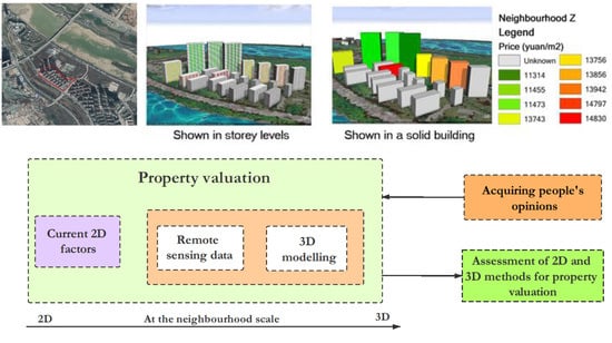
:Recent rapid population growth and increasing urbanisation have led to fast vertical developments in urban areas. Therefore, in the context of the dynamic property market, factors related to the third dimension (3D) need to be considered. Current hedonic price modelling (HPM) studies have little explicit consideration for the third dimension, which may have a significant influence on modelling property values in complex urban environments. Therefore, our research aims to narrow the cognitive gap of the missing third dimension by assessing both 2D and 3D HPM and identifying important 3D factors for spatial analysis and visualisation in the selected study area, Xi’an, China. The statistical methods we used for 2D HPM are ordinary least squares (OLS) and geographically weighted regression (GWR). In 2D HPM, they both have very low R2 (0.111 in OLS and 0.217 in GWR), showing a very limited generalisation potential. However, a significant improvement is observed when adding 3D factors, namely view quality, sky view factor (SVF), sunlight and property orientation. The obtained higher R2 (0.414) shows the importance of the third dimension or—3D factors for HPM. Our findings demonstrate the necessity to include such factors into HPM and to develop 3D models with a higher level of details (LoD) to serve more purposes such as fair property taxation.
1. Introduction
In the last decades, rapid population growth and increasing urbanisation rates have led to fast vertical developments in urban areas on top of the horizontal sprawl in China [1,2]. The construction of high-rise buildings in urban areas is driven by limited land availability and growing urban population [3,4]. The spatial configuration of urban areas rapidly changes with their increasing densities and high-rise developments. Consequently, information on the vertical dimension is getting more important, for example, analysing changes in terms of view orientation, vision scope and sunlight direction. In the context of a booming property market, these 3D property characteristics should be considered as components for property value as well. Though property value refers to the estimated amount at which a property will be exchanged, in this research, property value refers to the first-hand transaction price in the market [5,6]. Generally, the property value is determined by factors from different categories, e.g., physical, locational, and environmental. Such factors are employed to model property values, e.g., using the hedonic price model (HPM) [7,8]. At present, geographical information system (GIS) and remote sensing data are widely used because they provide abundant spatial information, which can be interpreted to estimate the influences of different factors on property values. However, their integration and involved factors are mainly 2D-based [9,10,11], while 3D factors have not received much attention. Reasons relate to difficulties of quantifying them, and the computational complexities, e.g., modelling view changes on different storeys, such as the sky view factor (SVF) [12,13,14]. Therefore, in this paper, we attempt to narrow the gap of the missing third dimension in HPM by assessing both 2D and 3D models and identifying important 3D factors for spatial analysis and visualisation.
Apparently, 2D methods are incapable of describing 3D characteristics in detail and do not provide precise differences between properties at different storeys when handling the complexity of vertical developments in urban areas. In contrast, 3D modelling can visualise the spatial relationships in the vertical dimension and support realistic simulations. Thus, it interacts with people better and provides a more in-depth understanding of the complex urban environment compared to 2D display [10,15,16]. Such 3D models have been implemented in multiple domains for solving problems such as building reconstruction and sunlight direction simulation [17,18]. For example, SVF, an important factor measuring sky visibility, is widely used to study the relationship between urban morphology and urban heat island (UHI) [19]. It is mainly determined by building height and regional building density, both factors related to 3D. It measures residents’ living comfort to some extent in densely-populated urban areas. In terms of sunlight, better sunlight condition means more daylight hours, less energy consumption and more comfortable living experience [20]. Although there have been many empirical studies related to 3D modelling, only a few studies have explored and visualised the importance of 3D factors concerning HPM for property values [21,22,23]. For example, the building height was proven to impact the property values in high-rise buildings in Hong Kong: properties on a higher storey level (above 20th) were more popular than those on a lower storey level (under 10th) [24]. There are studies investigating specific 3D factors in property values. Yamagata et al. [25] evaluated the values of city views categorised in dummy variables. They found a “very nice” open view and ocean view impact positively, whereas “poor” and “too much” green view might reduce the value. Sander and Polasky [26] defined a complex variable matrix, including dummy variable, percentage of a viewshed, and Euclidean distance, to calculate viewshed area, view quality, and view richness. However, they lack the spatial analysis of a real 3D environment. Therefore, the literature gap leaves us with questions about which 3D factors influence property values and if remote sensing data can be beneficial as input data for 3D spatial analyses. In general, 3D factors could have a high potential to increase our understanding of the importance of them in property values and stimulate new solutions to current-existing problems in a complex urban environment with generous amounts of high-rise buildings. The gap between the importance of the third dimension and its absence in the current HPM studies is identified.
In Xi’an, China, the first-hand property values have experienced a significant increase since 2018 [27]. As a result, the government has established fixed-price and purchase-restriction policies for market stabilisation. The general procedure is that the real estate developers declare the property value to the government first, and they are only allowed to start sales after the approval by the government. In other words, the first-hand values are determined by the government according to the local market conditions; thus, the first-hand property market is highly-restricted. In contrast, the second-hand property market is free and excessively prosperous because more profits can be made as compared to the first-hand value, which is generally lower than the market rates.
This research is conducted at the neighbourhood scale. We compared two HPM, one with 2D factors and one with 3D factors, to investigate which one shows a better performance to estimate property values (to increase the readability, they are abbreviated to 2D model and 3D model respectively in the following sections). The 3D simulation and 3D modelling workflow can provide valuable insights into future research for HPM of high-rise urban residential buildings.
The rest of this paper is organised as follows. Section 2 describes the overall methodology framework, followed by an overview of the study area and data sources. Then methods applied in different stages are presented in detail. Section 3 shows the results regarding 2D and 3D model results and the model performance assessment. Section 4 provides discussions relating key literature to the main findings in this research, mainly stressing the importance of involving 3D factors. Conclusions and future recommendations are outlined in Section 5.
2. Materials and Methods
We applied a mixed qualitative-quantitative methodology (Figure 1). Expert interviews, focus group discussions and questionnaires were conducted to understand policies related to the property market in Xi’an and determine the factors influencing property values which were categorised into 2D and 3D factors subsequently. Specifically, the answers from interviews and focus group discussions affected the questions in the quantitative questionnaires. For example, we took only the factors emphasised in interviews and focus group discussions in questionnaires, so that we have a limited number of factors but with high importance. The regressions of the 2D model included ordinary least squares (OLS) and geographically weighted regression (GWR). Only OLS was applied for the 3D model due to the relatively small sampling size (60 samples). Model validation was performed for checking the 3D model robustness. Finally, we assessed the statistical results of 2D and 3D models and analysed the added values of 3D factors.
The most commonly used of the three key valuation methods for valuing residential properties is the comparative method [28]. When using the comparative method, the valuers rely on their knowledge, experience and expertise to identify the comparable properties, whose characteristics are then compared to the subject property, with those of the subject property allocated values. Though these allocated values of the characteristics of the subject property are not stated, the final estimated value of the subject property is given. The comparative method though a form of hedonic pricing, does not show the ascription of the characteristics of the property. However, the regression models here attempt to mimic the valuer’s thought process explicitly. These factors are hence key to the valuation and HPM process. Here we define several terminologies used in this research. 2D factors are those influencing the values on planar bases such as accessibility to public facilities and the surrounding environment. 3D factors are those linked to building height and influencing the values on the vertical dimension (e.g., sunlight and SVF). The property values are the first-hand transaction price of the properties, and the unit is yuan/m2. In the regression, these factors are input as independent explanatory variables and the property value as the dependent variable. The neighbourhood in Chinese contexts refers to a residential district (usually enclosed by the walls and gates in urban areas), which consist of several residential buildings (the number can range from single digits to hundreds) and different living facilities (e.g., green belts, parking lot, playground) [29]. It should be noted that the area coverage of each neighbourhood varies significantly.
2.1. Study Area
Xi’an, the capital of Shaanxi Province, is located at Guanzhong Plain (Figure 2a). It is the educational, political and economic centre of northwest China. It is chosen as the study area because enormous property market changes have been recently observed [30]. The population reached 10.37 million in 2018 [27]. With an annual population growth of 6.6% between 2016–2018, there have been a large number of constructions of new high-rise neighbourhoods to shelter the influx of people, which results in a significant change in the city’s skyline, coupled with a flourishing property market and its accompanying skyrocketing property values [31].
In general, this research can be divided into two parts, 2D and 3D property value model. The 2D model takes neighbourhoods with first-hand property values established in 2018 in Xi’an urban areas (excluding country regions) as study objects. The 3D model is generated at the neighbourhood scale to make data collection feasible because investigating the influence of 3D factors is both computational costly and time-consuming. Two residential neighbourhoods, abbreviated as “Y” and “Z”, were selected (Figure 2b). The selection was motivated by the following facts: (1) both started constructions in 2018 and thus only contained properties in roughcast conditions, avoiding the influence of decoration levels on the values. Normally, properties with decorations have higher values compared to the roughcast ones when they are in similar conditions [32]. Regarding second-hand properties, it is hard to distinguish the sources of influences: whether it comes from different decoration levels or from the third dimension; (2) both contained sufficient samples of first-hand property values while other neighbourhoods lack sufficient data for the minimal conditions of running statistical regressions [33]; (3) both only had high-rise buildings in their neighbourhoods, so we could exclude the influence from low-rise buildings, terraces or houses. Furthermore, the selection was also advised by the respondents (e.g., real estate sales managers and university professor) we interviewed at Xi’an. The administrative district both are located in is a normal district in Xi’an, which is not too remote from the city centre and consists of new buildings. Regarding the neighbourhoods, they were designed as a standard residential area. The residents in these neighbourhoods are middle-income class.
2.2. Data Source
The different data was collected from several sources (Table 1). It included remote sensing data, vector data of Xi’an, and property value databases. A Sentinel-2 satellite image taken on the 26th of October, 2018 was used. After preliminary data quality controls, this image was taken in autumn, which has enough vegetation cover in Xi’an; while other images taken at similar times had issues such as higher cloud coverage and incomplete coverage of the study area. A Gaofen-2 satellite image was taken on the 12th of April, 2017 with a 4 m resolution, enough for land cover classification within the scope of this research. A Google Earth image taken on the 24th of April, 2017 was used for the following reasons: (1) it had no cloud coverage; (2) the image resolution was optimal for visual validation, i.e., selecting reference points for accuracy assessment of the land cover classification; (3) it was one of the newest images suitable for comparison when the research was conducted. The floor numbers of the buildings in Xi’an were obtained through applying open-source crawlers to online navigation platform, such as AutoNavi, established by AutoNavi Software Co., Ltd. (https://mobile.amap.com/). The crawler tools are only for education and research purposes. The property market was under fixed-price and purchase-restriction policy, which meant the values were controlled by the government, rather than real estate developers. Therefore, we decided to use first-hand property values rather than second-hand property values as in other HPM studies for the following reasons: (1) The first-hand property values were registered and published by the Price Bureau of Xi’an. They were grouped by the neighbourhood, released at the level per property in a well-organised form. Thus, they had less noise (as compared to the second-hand records), high data reliability and accessibility. (2) Based on our observations, as well as suggested by various property professionals we interviewed, the second-hand property market was over-heated at that time. It happened because the first-hand property values were controlled by the government, which caused an inflation of the second-hand property values. This phenomenon led to a large increase in second-hand property values within a few months. Hence, it was hard to identify and separate the real influences of 3D factors. (3) Different decoration levels influence the second-hand property values considerably, which is very typical in the Chinese context and partially different from Western countries. For example, properties with similar locational and environmental attributes can be sold with entirely different values if one is equipped with luxury furniture and another is poorly decorated. Different decoration styles mean different Fengshui (geomancy), which is highly appreciated and emphasised in Chinese traditional culture [30,31]. Nevertheless, it is difficult to observe whether a specific property is accompanied by appreciated or depreciated Fengshui only from property values. This fact was confirmed by the real estate sales managers we interviewed. (4) The second-hand records had noises (e.g., only a few samples inside one neighbourhood or missing physical attributes) and the validity was another critical issue to be concerned. In summary, we decided not to use noisy second-hand data because we want to see the impact of 3D factors, and therefore the less noisy first-hand data is more appropriate. There were 298 samples in the database of the first-hand property value of Xi’an in 2018 (average per neighbourhood) used for building 2D model. The samples covered the period from the 1st January, 2018 to the 18th September, 2018. Each neighbourhood was represented by the point at its centre. The coverage included seven urban administrative districts, excluding the county regions not under the purchase-restriction and fixed-price policy.
2.3. Expert Interview, Focus Group Discussion and Questionnaire
We organised expert interviews, focus group discussions and questionnaires to investigate the policy background of the property market in Xi’an and the preferences of local residents for high-rise residential buildings. Consent forms were signed by the respondents, and they were well-informed about the research contents orally before participation. Semi-structured expert interviews allowed us to gain contextual knowledge of the study area [34]. In total, eight interviews were held and twelve interviewees were involved, with diverse expertise including sales managers and architecture design directors from real estate developers, engineers from survey and mapping institutions, a university professor specialising in land administration, and managers from the urban planning sector. We asked them to describe the property characteristics valued by buyers and the reasons behind, to explain the current policies related to the first-hand property market, to introduce the general pricing policy of real estate developers, and to describe if and how the third dimension was being considered in Xi’an. The interview transcripts were used to select 2D and 3D factors included in the questionnaire for local residents. We conducted two focus group discussions, with a total of 10 ordinary buyers. The overall aim was to obtain property-related information from buyers, rather than from expert perspectives.
Questionnaires were used to investigate local residents’ preferences for high-rise residential buildings. We issued both online and paper-based questionnaires to cover different groups of inhabitants (e.g., age ranges). The online version was issued via Wenjuanxing, a Chinese online survey software. The paper-based ones were distributed in several public spaces without picking up specific target groups. We received a total number of 142 filled-in questionnaires. The contextual questions contained multiple-choice and scoring questions to survey their preferences for identified 2D and 3D factors. The attitudes were measured under a five-point Likert scale, i.e., using the categories, which has been widely applied in survey research to quantify subjective feelings [35,36]. We ranked the importance of factors by total marks in descending order. The results were taken as a reference for factor selection in 2D and 3D models.
The audio recordings of interviews and focus group discussions were transcribed using ATLAS.ti 8 (from ATLAS.ti Scientific Software Development GmbH, Berlin, Germany), a computer-assisted software suitable for interpreting transcripts and executing qualitative analysis. The questionnaires were statistically analysed using the built-in functions in Wenjuanxing software.
2.4. Factors for 2D and 3D Models
Based on their importance rankings from questionnaires, the 2D and 3D factors to be used were identified. There were eleven factors in the 2D model (Table 2). Factories were defined to all manufacturers with mass productions. The density radius was set to 1 km after optimisation. We used Euclidean distance for all the locational attributes due to its straightforwardness, which is also a popular measurement in similar housing studies [37,38,39]. Drum Tower, a famous historic site located in the city centre, was set up as the only CBD. Xi’an has been developing sub-CBDs for diverse purposes, yet Drum Tower remains the most important one. NDVI was used to extract the amount of green area coverage inside the neighbourhood as a factor measuring one aspect of the living environment. It has been widely used in studies related to environmental conditions, e.g., urban heat island and thermal comfort [40,41]. As mentioned before, the neighbourhood size in China varies much, to not exceed the neighbourhood boundary, the radius was set to 50 m after optimisation. The mean NDVI value within a 50 m radius was used as the input in the 2D model.
In the 3D model, in total, four factors were selected (Table 3). View quality was defined as the proportion of the areas of positive view types, which are pleasing to the eye, to the total. The preferred orientation to be used for sunlight and property orientation was determined based on the questionnaire responses. The 3D modelling process can be found in Section 2.6.2.
2.5. Statistical Models for 2D: OLS and GWR
Based on the theories proposed by Rosen [7] and Lancaster [8], the hedonic price model (HPM) has been widely recognised as a consistent and general theoretical basis in current literature to estimate property values by deconstructing the property characteristics into different attributes [37,43]. The fundamental concept is that the property is regarded as a heterogeneous product, whose value consists of a complex variety of attributes (e.g., environmental, physical and locational attributes) [44,45]. The environmental attributes include the characteristics of the surroundings of the property (e.g., noise and air quality). The physical attributes consist of various property characteristics itself, such as the floor area, the size, the shape, and the number of rooms. The locational attributes include different geographical locations of public goods, the accessibilities and distances to a specified facility (e.g., bank, park, and hospital). Each attribute contributes to the total value. In HPM, the property value serves as the dependent variable, and different attributes of the property serve as independent explanatory variables. Two statistical models were applied in this research, namely OLS and GWR. OLS is a classic linear technique applied to build HPM, which requires explicit definitions of non-linearities and interactions [46]. Equation (1) shows as follows:
where represents the property value, represents the intercept value, represents the coefficient of the corresponding variable to be estimated, represents the corresponding variable, and is the error term.
However, OLS has been criticised for its multicollinearity issues, omitting variables, and possibly containing biased results [47,48], so in the current literature body it always serves as a basic model to be compared with other more advanced models (see papers as follows [46,49,50,51]. In contrast, GWR, a locally weighted regression model, is found to be advantageous over OLS in existing studies [38,52,53,54,55], highly appreciated for revealing the spatial heterogeneity in property values and the factors. It also has a better model performance and accuracy compared to OLS [56]. Currently, there are abundant housing studies adopting GWR as the main method. For example, Qu et al. [57] used GWR to explore the temporal variation of different factors on residential land prices and found that environment-related factors had positive influences on land prices. Li et al. [58] employed GWR to investigate the relationships between the number of microblogs and housing prices so that the local effects could be observed. Conceptually, GWR is a linear model assuming that the coefficient is a combined function of both the variable and its spatial coordinates. Different relationships between variables are allowed to exist across spaces. The calibration concept is based on the fact that the variables closer to the sample location have a greater influence on the local parameter estimates for that location. In this research, the fixed Gaussian function was selected as the spatial kernel type, and Akaike information criterion (AICc) was used to define the final bandwidth. The equations of GWR (Equation (2)) and Gaussian function (Equation (3)) are as follows:
where represents the property value at location , represents the intercept value, represents the coefficient of the th variable at location , represents the , coordinates of property at location , represents the value of the th variable at location , and is the error term at location .
where represents the weight for the kth variable at location i, represents the distance between the observations i and k, and h; represents the bandwidth.
2.6. Modelling 3D Factors
2.6.1. Workflow for 3D Modelling
The workflow mainly consists of five steps aiming to show and analyse influences of the third dimension to the property values (Figure 3). CityEngine was used for its capability of 3D spatial analysis and visualisation [10,59]. As neighbourhoods Y and Z were still under construction when the research was conducted, the buildings were invisible in the image. Resultantly, the footprints were drawn manually based on the remote sensing image (taken at the 28th of April, 2018) in Google Earth because it was the newest image which could be assessed.
Within Step 1, the size and orientation of the building footprints were adjusted in ArcMap; then, detailed attributes were assigned to them to build direct links when modelling in CityEngine in the later stage. Within Step 2, five land cover classes, namely paved, water, green, soil and building, were extracted from Gaofen-2 image using support vector machine (SVM). SVM is a robust machine learning algorithm and shows better accuracies than standard parametric image classifiers [60]. It only needs a relatively small amount of training samples and has a solid theoretical basis [61]. Visual interpretation based on Google Earth image was employed for validation. Two hundred random points were created and manually labelled. Generally, the target is to reach an 85% overall land cover classification accuracy [62]. Within Step 3, 3D scenes were built. The building footprints of the study neighbourhoods and data of the floor numbers of buildings in Xi’an were extracted by assigning rule files written in computer generated architecture (CGA), a programming language of CityEngine dedicated to generating architectural 3D content [10,63]. The storey height of all buildings was assumed to be 3 m, a common storey height of the residential buildings in China. Information about the floor numbers of buildings in Xi’an was extracted to reach LoD 1 in CityEngine. LoD 1, based on the literature, means simple blocks [64]. The building footprints for the study neighbourhoods were built in LoD 2, allowing the generalisation of the thematic roof features, windows, doors and façades. LoD 2 was appropriate for visualisation at the neighbourhood scale. Within Step 4, viewshed and sunlight analysis, two built-in functions in CityEngine, were applied to visualise and quantify the influences and changes of 3D factors and the values were exported and modelled in OLS via SPSS subsequently. The 3D models were exported to ArcGIS Online for users’ demonstration. Within Step 5, the 3D model validation. It has not been done in previous studies [14]. Leave-one-out cross-validation (LOOCV), a special case of leave-k-out cross-validation was applied. It leaves one sample for the test set at a time, and the other samples are used for the training set. If there are k samples, the train and test sets are both executed k times. It is cumbersome but has high sample-efficiency, suitable for small sampling size [65]. We accomplished the validation based on local knowledge since there was no similar model or technique available for comparison. The error is defined as the proportion of the standard deviation between the estimated value and the real value to the average property value. It was used to represent the estimation accuracy of the 3D model.
2.6.2. 3D Analyses in CityEngine
3D scenes under four view distances (50, 100, 200 and 500 m) were set up to analyse 3D factors comprehensively. The selection criteria of view distances were as follows. According to Chinese urban planning regulations, the distance between two residential buildings should be no less than 1.2 times the lower building [66]. The building heights in neighbourhoods Y and Z were 18 m, 54 m, 90 m, and 99 m. Therefore, the minimum view distance was approximately 50 m. 100 m was for the buildings with 90 m and 99 m high. Based on the literature, 500 m was set up to be the maximum for the following two reasons: (1) it is generally the farthest distance that people can see through [67] and (2) we found no significant differences of view areas and view types after 500 m, which means a set-up after 500 m may be meaningless. 200 m was set up as a medium distance.
As we explored 15 buildings with known property values in neighbourhoods Y and Z and built four scenes under different view distances, there were 60 samples in total for regression modelling. After optimisation, the 3D scene radius for each neighbourhood was set up to 1 km, an appropriate distance to capture the surrounding environment characteristics for visualisation [46], also meeting the requirements for 3D analyses and limited computation capacity. As property orientation was set as the dummy variable, which was not analysed in CityEngine, the parameter settings at below were for view quality, SVF and sunlight.
- View quality and SVF
The viewshed analysis visualised and quantified two factors, i.e., view quality and SVF, under the same parameter settings (Table 4). The observer was assumed to stand in the middle of the building for the fact that the average property value per building served as the dependent variable to represent the average value of view quality. The final values of view quality and SVF were the average value at four different view distances.
- 2.
- Sunlight
It was calculated using the built-in function in CityEngine, Scene Light and Panorama. To ease calculation, three representative timings were defined based on local knowledge: 8 A.M. when people go to work, 12 A.M. with the most intense sunlight, and 4 P.M. when the sun is about to set. We took the average value of the three timings to represent sunlight.
3. Results
3.1. 2D Models in OLS and GWR
3.1.1. The Comparison of OLS and GWR
In OLS, R2 and adjusted R2 are 0.111 and 0.077, respectively, which means it explains only approximately 10% of the property value variation. The low explanatory power of the model is caused by the strict government control of the first-hand property values; thus, the actual market demand and the influences from the surrounding geographical environment were not sufficiently represented. This provides an optimal base to analyse whether 3D factors can explain the property value variations existing in the first-hand property values. Five factors are significant at the 0.05 significance level: distance to CBD, distance to subway, distance to food, the density of factories and NDVI. The Durbin-Watson value is 1.890, close enough to the optimal value 2, which assumes the residuals are uncorrelated. Tolerances are all greater than 0.2, and variance inflation factors (VIF) range from 1 to 3, below the value of 10, indicating that no serious collinearity issue exists among these variables, which is suitable for executing GWR. In general, the model goodness-of-fit of OLS and GWR is not ideal, yet GWR still outperforms OLS, as adjusted R2 improves from 0.077 to 0.128, and R2 improves from 0.111 to 0.217. The residual sum of square (SSR) in GWR also significantly reduces from 3,392,667,848 in OLS to 2,655,158,522. Therefore, GWR is finally chosen to analyse the influences of 2D factors on property values.
3.1.2. GWR
Table 5 shows the descriptive statistics of GWR. Based on previous HPM studies [39,68], we used the 0.05 significance level as the critical value to determine whether this factor is statistically significant. β is the coefficient of each variable. Distance to CBD is the most significant among 11 factors, with a standardised coefficient of −4.880. It has a negative correlation with property values, meaning the smaller the distance to the CBD, the higher the property value. The density of bus stops only has a slightly positive standardised coefficient of 0.231. This may be because of the well-developed bus network in Xi’an. Distance to food has the most significant positive standardised coefficient of 2.695, which means the property value lifts as the distance increases. The environmental pollution caused by restaurants may partially explain it. Since the urban development in Xi’an is spatially unbalanced, the influences of 2D factors on property values vary significantly.
- Local R2
Local R2 ranges from 0.093 to 0.207, and the mean value is 0.124. As shown in Figure 4a, it increases from north to south gradually, indicating the model simulation in the south is better than that in the north. Some samples in the north area are found to have an abnormally low value. In reality, the urban development pattern of Xi’an shows great asymmetry. In the past decades, the south part has been more developed compared to the north. The north and east parts of Xi’an are less developed, where mainly infrastructure functions are located, such as transport, harbour affairs and industry. In the south-eastern region, there is a high concentration of educational facilities, shopping malls, world-famous historical sites such as Big Goose Pagoda, which positively influences property values. The south-western region, with the highest local R2, is the National High-tech Development District, having a cluster of high-tech industries and high-quality school districts, major hospitals and premium residential neighbourhoods.
- 2.
- Factories
Only one property in the north part has a positive coefficient of 22.264, which can be taken as an outlier. The remaining 297 locations all have negative values, ranging between −1585.278 and −22.264, with a mean value of −870.293. As the density of factories increases, property values decrease. 198 out of 298 samples, i.e., 66.44% are located in areas where there is less than the average of one factory within 1 km2. Twenty-seven samples, i.e., 9.06% are in areas with more than two factories within 1 km2—the absolute value of the coefficient increases from northeast to southwest. Property values in the southwest area are more likely to be influenced by the density of factories than those in the northeast. There are three greatly-agglomerated regions shown in blue (Figure 4b). However, these highly-dense industrial zones do not affect property values negatively based on the regression results.
- 3.
- Food
All coefficients are positive, from 1.488 to 9.706 and with a mean value of 5.455. It means that the farther from the food, the higher the property value. In total, 252 out of 298 locations, i.e., 84.56% have a distance less than 200 m, meaning easy food accessibility in most areas (Figure 4c). The general trend increases from south to north, indicating that properties in the north are more influenced than those in the south. The positive value may be because an area with many restaurants has a negative influence on the living environment concerning noise and public sanitation.
- 4.
- Subway
The coefficients range from −1.433 to −0.274, and the mean value is −0.701. The negative value indicates that the farther from the subway station, the lower the property value. In total, 63.09% and 26.51% of the property samples are located in the range of 0–1 km and 1–2 km. The majority are with reasonable distances of the subway (Figure 4d). From south to north, the coefficients gradually increase, indicating that the property values in the south are more influenced. It may be that the north area is relatively remote from downtown, and the public transport is not well-developed.
- 5.
- CBD
The coefficients range from −0.381 to −0.175, indicating the negative impact of distance to CBD on property values: the closer, the higher the values (Figure 4e). The mean value is −0.230. It is the most important among the five significant factors. A total of 224 out of 298, i.e., 75.16% are in the range from −0.25 to −0.15, which is highly centralised. Thus, residents in Xi’an prefer living near CBD, because of the living convenience and the symbolisation of high social status. Only the imperial family could live near the Drum Tower in ancient China. The coefficients increase from southwest to northeast, showing that property values in the southwest are more influenced by the distance to CBD than those in the northeast.
- 6.
- NDVI
Figure 4f shows that there is not much vegetation within the urban areas, while at the fringe of the city, the vegetation coverage increases gradually. The brown area is the Chan River. Only one sample shows a negative coefficient of −137.098, while the remaining are all positive with a range from 1967.216 to 6617.045. Thus, the higher the vegetation covers, the higher the property values. The coefficients increase from north to south. People’s housing preferences and the varying quality of the neighbourhoods may lead to this difference. It is worth mentioning that the majority of the neighbourhoods in this research are still under construction. Generally, the real estate developers in China start sales before the high-rise building construction starts. Thus, NDVI shows the vegetation’s current situation and its influence on property values, which may be subject to change in the future.
3.2. 3D Model and Visualisation
3.2.1. 3D Analysis
The land cover classification shows an overall classification accuracy of 87.5%, meeting the commonly employed threshold of 85%. Therefore, it is taken as input for building 3D scenes of the two neighbourhoods Y and Z, which are abbreviated to only Y and Z in the following sections for readability. Both scenes are published in ArcGIS Online (Y: http://bit.ly/2IEA3Wy; Z: http://bit.ly/2Iyl4NJ.). Figure 5 takes Z as an example, showing the building distribution and the fact that property values increase as building heights decrease.
- View quality
The land cover classes “green” and “water” are defined as positive view types as they receive the most votes from the questionnaires. As shown in Figure 6, view quality between different buildings fluctuates significantly. Generally, as view distance increases, view quality improves. The possible reason can be more view areas and view types are included when having an extended view distance. For example, when the view distance is 50 m, only adjacent buildings and the panorama are typically visible, so many buildings have zero value. However, including more view areas does not mean always improving the view quality. It is notable that unlike other buildings, Z_01 and Y_10 have a decreasing trend after 50 m and 100 m, respectively. Although the positive view areas of green and water improve, view areas of road, building and soil increase more; for others, view quality improves along with the increase of view distance. The average values of Y and Z are 0.049 and 0.095, respectively; thus, Z has a better view quality than Y.
- 2.
- SVF
It is evident that as view distance improves, SVF decreases because adjacent buildings block most of the sky (Figure 7). Y has relatively high SVF because all buildings are more than 30 storeys. The higher the building, the harder it can be blocked by surrounding environments. The same situation is also observed in Z. Z_1, Z_5, Z_6 and Z_7 with the building height of 54 m, have an average SVF of 0.463; while Z_2, Z_3 and Z_4, with the building height of 99 m, have an average SVF of 0.632. The least value (0.250) belongs to Z_09 and Z_12, both with a height of 27 m. The average SVF values of Y and Z are 0.486 and 0.472, respectively. In general, Y has better SVF than Z. It can be concluded that SVF increases with the building height.
As shown in Figure 8, SVF changes both with building locations and view distances. SVF of Y_06 is relatively good, all above 0.5 with an open space in the south. SVF of Y_08 is below 0.2 because Y_06 blocks Y_08 in the south. As view distance increases, SVF gets smaller due to the increase of other view types in the viewshed.
- 3.
- Sunlight
Derived from the questionnaires, 137 out of 141 responses select south as the best orientation for the main rooms of a property. Therefore, we choose the south orientation to calculate sunlight. In both neighbourhoods, no high buildings exist in the surrounding environment within 1 km, so sunlight is only blocked by buildings in the same neighbourhood (Table 6). Most of the buildings cannot receive direct sunlight at 8 A.M. in both June and December. Only Z_01 and Z_12 have properties which can get direct sunlight. All buildings receive direct sunlight in June (12 A.M.); however, the results at December (12 A.M.) vary much due to the block from other buildings. The low values in December (4 P.M.) of three buildings, Y_08, Y_09 and Y_11, are also because of the block. Notably, Z_09 and Z_12 have the smallest total values. The possible reason may be that they only have nine storeys, 27 m high, and the shadow from other buildings can easily block the sunlight. The average values of Y and Z are 0.543 and 0.525, respectively. Y has slightly better sunlight conditions than Z.
West–east orientation is disliked due to west sun exposure according to the responses from focus group discussions and questionnaires. A specific simulation is shown in Figure 9. Y_08, Y_10 and Y_11, three buildings with green colour, are fully exposed while some properties in Y_07 and Y_09 with red colour are under the shadow of other buildings. It shows that properties with less west sun exposure have higher values. It is also remarkable that Y_06, having west sun exposure, still has high property values. Other factors, such as view quality, may influence this because the south of Y_06 is an open space without any blocks from buildings.
- 4.
- Property orientation
As mentioned before, nearly all buyers (137/141) in the questionnaire prefer south orientation, so we put south orientation as the preferred orientation. There are two orientations involved in Y and Z, south and east–south. Therefore, south orientation equals one while east-south orientation equals zero.
3.2.2. Statistical Analysis of the 3D Model
As shown in Table 7, R2 (0.451) and adjusted R2 (0.411) are much higher than those of 2D models. The residual is 125,452,566.4. The Durbin–Watson value is 0.432, indicating positive autocorrelation in the samples. It is likely to be because the samples are repeatedly calculated under four different view distances. Tolerances are all greater than 0.2, and VIF ranges from 1 to 3, far less than 10; thus, no serious collinearity issue exists among factors.
SVF and sunlight are both statistically significant at the 0.05 significance level. Property orientation is the most significant one among the four factors and significant at the 0.01 significance level. Surprisingly, property orientation has a negative standardised coefficient of −0.792, indicating the values decrease when facing south. It may be because the buildings with nine storeys facing southeast in Z have relatively higher values. Sunlight has the second most significant standardised coefficient of 0.327. When there is more sunlight, the value is higher. The standardised coefficient of SVF is −0.271, implying that as SVF improves, the value decreases, which is reflected by the simulation results that buildings with more storeys have a broader vision scope than those with fewer storeys. The only insignificant factor is view quality, with a significance of 0.300 and the standardised coefficient of −0.123. The possible reasons are elaborated in Discussions.
3.2.3. Model Validation
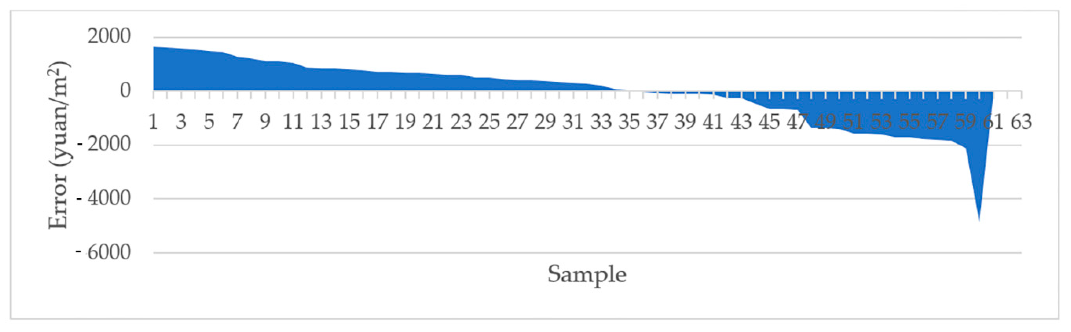
Twenty-five samples have an estimated value lower than the real value, while 35 have a higher one (Figure 10). 36 out of 60 samples have the absolute value of error of less than 1000 yuan/m2. Notably, one sample has a maximum error of −4864 yuan/m2. It is Z_09, the building with nine storeys, and 27 m high when the view distance is 50 m. It may be explained by poor SVF and view quality.
Buildings with higher heights are estimated to have higher values, such as Y_08, Y_10, Y_11, and Z_04. The top ten with the most positive error are the buildings with 33 storeys, and 99 m high for having better performances at view quality, SVF, and sunlight. Z_05, Z_06, Z_07, with 18 storeys, and 54 m high, have a relatively higher negative error. The average deviation is 1219.294 yuan/m2, and the average error of estimation accuracy is 9.76%.
3.3. Model Performance Assessment
As shown in Table 8, R2 of the 3D model is the highest (0.451), indicating the 3D model explains the property value variation better than 2D models at the neighbourhood scale. SSR also shows a significant decrease to 125,452,566.
4. Discussions
4.1. Current Restricted Property Market and HPM with 2D Factors
Previous studies have indicated that HPM with 2D factors well explain the property value variation [26,69], while our paper proves that 2D models do not explain the first-hand property value variation in Xi’an. Currently, the property values are generated under the fixed-price and purchase-restriction policies established by the government aiming for market stabilisation. Therefore, impacts from the surrounding environments on property values are likely to be implicit. The low explanatory power of R2 in both models may serve as a reference for policy-makers: before implementing a housing policy, the possible subsequent implications may be significant: in this case, the influences from the surrounding geographical environment are almost eliminated, and the actual market demand cannot be reflected. Such kinds of consequences should be taken into consideration and well-addressed before establishment. GWR outperforms OLS with a higher R2, which is consistent with previous findings [53,70]. However, the significance of 2D factors differs from previous literature. For example, in Wen et al. [54], educational facilities had a positive influence, while this was not the case in this research. The accessibility of parks did not show a significant influence on property values in this research, which differs from the findings of Jim and Chen, where it showed significantly positive impact that the less the distance, the higher the property values [71]. This research clearly shows the variations among factors influencing property values across different areas.
We would like to highlight that there are different proxies for the 2D factors, i.e., the calculation methods of these factors. Taking distance as an example, we applied Euclidean distance to different locational attributes as the calculation method for the following two reasons: (1) this calculation is theoretically simple and straightforward; (2) according to the local contexts, due to the fast city expansion, the current road networks of Xi’an have not finalised and are subjective to changes in the future. The distance can also be calculated in network distance (using the primary/secondary roads) [72], or travel time [73,74]. Therefore, we advise that in future studies, the proxies for 2D factors such as the distance should be selected carefully according to the research purpose and scale. For example, more behaviourally-relevant studies may adopt travel time for distance calculation.
4.2. Hedonic Price Model (HPM) with 3D Factors
View quality, with positive view types of green and water, does not have a significant influence on property values, which conflicts with Wen et al. [14], and Panduro and Veie [75] who found that both river and urban green spaces impacted positively. Jim and Chen [71] defined a dummy variable for different view types. In contrast, the view area is directly used in this research, which may impact the results. The insignificance can be explained by two main aspects: data and the local contexts of Xi’an. Regarding data, first, the sampling size (60) is relatively small due to data availability (see Section 2.1 for our selection criteria), so the variation of view quality is not very large, ranging from 0 to 0.32. Second, it may be influenced by other 3D factors. For example, view quality varies when different property orientations (e.g., orienting north other than south) are set up. Regarding the local context of Xi’an, first, unlike western cities with lower development speed and higher environmental quality maintenance (such as Aalborg, Denmark [75]), Xi’an is a fast-developing city with over 10 million population. It is also different from Hangzhou [14] or Hong Kong, China [71]. Hangzhou is a very famous city with an established reputation of its water landscape, also in a more advanced city development stage than Xi’an. Hong Kong has been an international, well-developed and densely built-up city for decades, where the green spaces (e.g., public parks) are generally fixed, and the water quality is well-regulated. In contrast, we have a different situation in Xi’an. The city is growing rapidly. There are green spaces, but they may be very easily and quickly developed. Due to the fast developments, a person may not value the existence of a green view to an open space which means vacant land. Vacant land means it will be developed, but we do not know how it will be developed- whether it will become a building, a factory or a park. In other words, if a person has a green view on vacant land, which will be soon developed, it will have an adverse influence on property values. However, investigating the sub-types of green spaces are out of the scope of our research. Similarly, water (e.g., river, lake) can be very positive if it is nicely maintained for the surrounding environment, but it can also have some issues with pollution. Previous studies in Guangzhou, China have proven that water with polluted quality reduced property values [39,76]. The fast-developing speed of Xi’an undoubtedly raises the uncertainty of quality maintenance and environmental protection. In conclusion, the overall influence may lead to an insignificant influence of view quality on property values. Furthermore, our study is on a small scale with a few buildings in two high-rise neighbourhoods.
The south orientation has a negative effect on property values, which is inconsistent with Jim and Chen [12], in which a south-oriented window added 1% premium of the value. It may result from the fact that only two orientations (south and southeast) exist in Y and Z, while six were reported in Jim and Chen [12]. SVF is found to impact negatively, which contradicts the common sense that buildings with higher SVF shall have higher values. In light of the general pricing policy of real estate developers, values of relatively low-rise buildings are higher than the high-rise ones, partly for better living privacy because usually fewer properties and larger property size are characterised in low-rise buildings. For example, the 9-storey-high building (Z_9, Z_12) has 18 properties, while the 33-storey-high one (Z_2, Z_3, and Z_4) has 232 properties in total. The property values of Z_9 and Z_12 are significantly higher than those of Z_2, Z_3 and Z_4.
Only 17% of respondents from the questionnaires prefer properties at a low storey level due to less sunlight exposure, in line with the finding that sunlight impacts positively on property values. Fleming et al. [77] also found that there was a positive relationship between sunlight exposure and property value. It is worth pointing out that sunlight is partially influenced by the property orientation in this research.
The error of estimation accuracy in the 3D model is 9.76%. In other words, the 3D model can estimate the property value within a fluctuation of approximately 10%. It is not a very large error, though, no existing studies have ever validated a 3D modelling method for HPM; thus, we have no comparison to set a specific threshold value yet. The authors agree that validation remains an issue to be solved [78]. Therefore, other validation methods should be researched in the future. Additionally, we would like to highlight that the visualisation of property values (Figure 5) is generalised to per building, as we use the average property values per building and the research is at the neighbourhood scale. When the scale can be further refined in the future, the representation is optimal to be in per property/floor.
The findings disclose that added 3D factors explain the property value variation at the neighbourhood scale better than 2D models, shown by a higher R2 (0.414) and fewer residuals. The 3D visualisation in CityEngine also performs well in terms of quantifying and spatially analysing 3D factors. We believe that making the 3D factor explicit can enrich the standard literature of HPM at the city scale, and even possible to activate academia’s attention to how 3D should be perceived in complex urban areas. Because of computational complexity, we used a smaller study area in this research, where first-hand property values are available and more appropriate to avoid too many noises brought by the second-hand property values. Nevertheless, we ultimately aim to apply this method to a city scale.
5. Conclusions and Future Recommendations
This research aimed to identify the role of the third dimension in property value calculation in a complex urban environment, taking the city Xi’an, China, as the study area. It was conducted at a neighbourhood scale and took spatial data from various data sources. The mixed-qualitative–quantitative methodology ensured comprehensiveness by collecting both subjective opinions and objective modelling. Based on low R2 of 2D models, we can summarise that when the first-hand property market is restricted by the government, property values do not reflect the influences from the surrounding environments well. Based on 3D modelling results, we observed that significant spatial heterogeneity exists in the vertical dimension, which influences property values considerably. Hence our findings show the necessity to include 3D factors into HPM and to develop 3D models with a higher level of details (LoD) to serve more research purposes such as fair property taxation.
A healthy property market is essential for a sustainable economy and a stable society. In China, rapid urbanisation leads to property market flourishment and increasing property values, which poses a long-term impact on people’s daily lives [79]. The high-rise residential building has been the predominant housing type in most urban regions. Therefore, it is essential to develop a comprehensive, fair and cost-effective method to estimate property values, which can be a reference to other Asian regions/countries sharing similar dense urban morphology and housing issues. Current HPM methods mainly adopt 2D-based data and workflow without considering the spatial heterogeneity in the vertical dimension and the influences on property values. Thus, our research contributes to the limited body of studies that investigate 3D in HPM. We observe that the integration of GIS, remote sensing data and 3D modelling for HPM are feasible and practical. Having the 3D model representing the buildings and environment realistically provides rich opportunities for precise analysis of the impact from the third dimension on property values.
Further research aiming to validate the 3D model and expanding the research may consider the following facts. First, four 3D factors are involved in total. If more factors (e.g., shadow, thermal comfort, air quality, noise, ventilation) or a city-scale research are considered, it would be beneficial to apply automatic rather than manual validation. Second, 60 samples are suitable for LOOCV, but the expansion needs large sample sizes. The validation method may change, as well. Third, the digital elevation model is not taken into consideration in the current 3D analysis. Fourth, 3D workflow optimisation by machine learning is encouraged to facilitate estimation accuracy and modelling efficiency. It is also worth to mention that big difference exists in values between buildings with different heights, property sizes and the total number of properties in one building. Therefore, it may need a tuning parameter to set a value basis for the buildings with different physical structures to compensate for their influences in the future. We should also acknowledge the fact that this research is constructed at the neighbourhood scale, which ignores on which storey property is located due to data availability. It, to some extent, reduces the added value of true 3D models as it attaches great importance to issues regarding sunlight and view.
Author Contributions
Conceptualisation, Y.Y., M.K. (Mila Koeva) and M.K. (Monika Kuffer); methodology, Y.Y., M.K. (Mila Koeva) and M.K. (Monika Kuffer); software, Y.Y.; validation, Y.Y.; formal analysis, Y.Y.; funding acquisition, Y.Y.; visualization, Y.Y.; writing—original draft, Y.Y., M.K. (Mila Koeva), M.K. (Monika Kuffer) and K.O.A.; review and editing, Y.Y., M.K. (Mila Koeva), M.K. (Monika Kuffer), K.O.A. and J.Z.; supervision, J.Z.; fieldwork support, X.L. All authors have read and agreed to the published version of the manuscript.
Funding
Y.Y. is funded by China Scholarship Council (CSC) under the grant number [201906560015].
Informed Consent Statement
Informed consent was obtained from all respondents involved in the study.
Data Availability Statement
The data presented in this study are available on request from the corresponding author. The data are not publicly available due to the confidentiality agreement with the data provider.
Acknowledgments
We would like to thank Jiong Wang for data support. We also thank all the respondents from expert interviews, focus group discussions for their valuable ideas and suggestions.
Conflicts of Interest
The authors declare no conflict of interest.
References
- Feng, Q.; Wu, G.L. Bubble or riddle? An asset-pricing approach evaluation on China’s housing market. Econ. Model. 2015, 46, 376–383. [Google Scholar] [CrossRef]
- Smith, K.; Liu, S.; Liu, Y.; Liu, Y.; Wu, Y. Reducing energy use for water supply to China’s high-rises. Energy Build. 2017, 135, 119–127. [Google Scholar] [CrossRef]
- Tavernor, R. Visual and cultural sustainability: The impact of tall buildings on London. Landsc. Urban Plan. 2007, 83, 2–12. [Google Scholar] [CrossRef]
- Liu, Z.; Zhao, X.; Jin, Y.; Jin, H.; Xu, X. Prediction of outdoor human thermal sensation at the pedestrian level in high-rise residential areas in severe cold regions of China. Energy Procedia 2019, 157, 51–58. [Google Scholar] [CrossRef]
- Ying, Y. Assessment of 2D and 3D Methods for Property Valuation Using Remote Sensing Data At the Neighbourhood Scale in Xi’an, China. Master’s Thesis, Faculty ITC, University of Twente, Enschede, The Netherlands, 2019. [Google Scholar]
- International Valuation Standards 2020; Page Bros: Norwich, UK, 2020.
- Rosen, S. Hedonic prices and implicit markets: Product differentiation in pure competition. J. Political Econ. 1974, 82, 34–55. [Google Scholar] [CrossRef]
- Lancaster, K.J. A new approach to consumer theory. J. Political Econ. 1966, 74, 132–157. [Google Scholar] [CrossRef]
- Wyatt, P.J. The development of a GIS-based property information system for real estate valuation. Int. J. Geogr. Inf. Sci. 1997, 11, 435–450. [Google Scholar] [CrossRef]
- Zhang, H.; Li, Y.; Liu, B.; Liu, C. The application of GIS 3D modeling and analysis technology in real estate mass appraisal—Taking landscape and sunlight factors as the example. In Proceedings of the The International Archives of the Photogrammetry, Remote Sensing and Spatial Information Sciences, Suzhou, China, 14–16 May 2014; Volume XL, pp. 363–367. [Google Scholar]
- Zhu, Q.; Hu, M.; Zhang, Y.; Du, Z. Research and practice in three-dimensional city modeling. Geo Spat. Inf. Sci. 2009, 12, 18–24. [Google Scholar] [CrossRef]
- Jim, C.Y.; Chen, W.Y. Impacts of urban environmental elements on residential housing prices in Guangzhou (China). Landsc. Urban Plan. 2006, 78, 422–434. [Google Scholar] [CrossRef]
- Yu, S.-M.; Han, S.-S.; Chai, C.-H. Modeling the value of view in high-rise apartments: A 3D GIS approach. Environ. Plan. B Plan. Des. 2007, 34, 139–153. [Google Scholar] [CrossRef]
- Wen, H.; Xiao, Y.; Zhang, L. Spatial effect of river landscape on housing price: An empirical study on the Grand Canal in Hangzhou, China. Habitat Int. 2017, 63, 34–44. [Google Scholar] [CrossRef]
- Van Lammeren, R.; Houtkamp, J.; Colijn, S.; Hilferink, M.; Bouwman, A. Affective appraisal of 3D land use visualization. Comput. Environ. Urban Syst. 2010, 34, 465–475. [Google Scholar] [CrossRef]
- Onyimbi, J.R.; Koeva, M.; Flacke, J. Public participation using 3D city models. GIM Int. 2017, 31, 29–31. [Google Scholar]
- Biljecki, F.; Ledoux, H.; Stoter, J. An improved LOD specification for 3D building models. Comput. Environ. Urban Syst. 2016, 59, 25–37. [Google Scholar] [CrossRef] [Green Version]
- Gimenez, L.; Robert, S.; Suard, F.; Zreik, K. Automatic reconstruction of 3D building models from scanned 2D floor plans. Autom. Constr. 2016, 63, 48–56. [Google Scholar] [CrossRef]
- Ha, J.; Lee, S.; Park, C. Temporal effects of environmental characteristics on urban air temperature: The influence of the Sky View Factor. Sustainability 2016, 8, 895. [Google Scholar] [CrossRef] [Green Version]
- Yu, X.; Su, Y. Daylight availability assessment and its potential energy saving estimation-A literature review. Renew. Sustain. Energy Rev. 2015, 52, 494–503. [Google Scholar] [CrossRef]
- Isikdag, U.; Horhammer, M.; Zlatanova, S.; Kathmann, R.; van Oosterom, P. Utilizing 3D building and 3D cadastre geometries for better valuation of existing real estate. In Proceedings of the FIG Working Week 2015 ‘From the wisdom of the ages to the challenges of modern world’, Sofia, Bulgaria, 17 May 2015; pp. 17–21. [Google Scholar]
- Tomić, H.; Roić, M.; Ivić, S.M. Use of 3D cadastral data for real estate mass valuation in the urban areas. In Proceedings of the 3rd International Workshop on 3D Cadastres: Developments and Practices; van Oosterom, P., Ed.; International Federation of Surveyors, FIG: Copenhagen, Denmark, 2012; pp. 73–86. [Google Scholar]
- Kara, A.; van Oosterom, P.; Çağdaş, V.; Işıkdağ, Ü.; Lemmen, C. 3 Dimensional data research for property valuation in the context of the LADM Valuation Information Model. Land Use Policy 2020, 104179. [Google Scholar] [CrossRef]
- Hui, E.C.M.; Zhong, J.W.; Yu, K.H. The impact of landscape views and storey levels on property prices. Landsc. Urban Plan. 2012, 105, 86–93. [Google Scholar] [CrossRef]
- Yamagata, Y.; Murakami, D.; Yoshida, T.; Seya, H.; Kuroda, S. Value of urban views in a bay city: Hedonic analysis with the spatial multilevel additive regression (SMAR) model. Landsc. Urban Plan. 2016, 151, 89–102. [Google Scholar] [CrossRef]
- Sander, H.A.; Polasky, S. The value of views and open space: Estimates from a hedonic pricing model for Ramsey County, Minnesota, USA. Land Use Policy 2009, 26, 837–845. [Google Scholar] [CrossRef]
- Xi’an Municipal Bereau of Statistics. Xi’an Statistics Yearbook 2018; China Statistics Press: Xi’an, China, 2019.
- Lisi, G. Property valuation: The hedonic pricing model—location and housing submarkets. J. Prop. Invest. Financ. 2019, 37, 589–596. [Google Scholar] [CrossRef]
- Liang, X.; Liu, Y.; Qiu, T.; Jing, Y.; Fang, F. The effects of locational factors on the housing prices of residential communities: The case of Ningbo, China. Habitat Int. 2018, 81, 1–11. [Google Scholar] [CrossRef]
- Lei, J. The Operation Situation of Xi’an Property Market in 2018. Chinese Business View. 2018. Available online: http://news.hsw.cn/system/2018/1122/1042031.shtml (accessed on 10 November 2020).
- Hurun Global House Price Index was Released and Xi’an Enters Top Ten; Hurun Research Institute: Shanghai, China, 2018. Available online: http://www.hurun.net/CN/Article/Details?num=61C2A98F9932 (accessed on 10 November 2020).
- Hu, L.; He, S.; Han, Z.; Xiao, H.; Su, S.; Weng, M.; Cai, Z. Monitoring housing rental prices based on social media:An integrated approach of machine-learning algorithms and hedonic modeling to inform equitable housing policies. Land Use Policy 2019, 82, 657–673. [Google Scholar] [CrossRef]
- Field, A. Discovering Statistics Using SPSS, 3rd ed.; SAGE Publications Ltd.: London, UK, 2009; Volume 58, ISBN 9781847879073. [Google Scholar]
- Sander, E.; Libby, J.; Caza, A.; Jordan, P.J. Psychological perceptions matter: Developing the reactions to the physical work environment scale. Build. Environ. 2019, 148, 338–347. [Google Scholar] [CrossRef]
- Liu, F.; Kang, J. Relationship between street scale and subjective assessment of audio-visual environment comfort based on 3D virtual reality and dual-channel acoustic tests. Build. Environ. 2018, 129, 35–45. [Google Scholar] [CrossRef]
- Clifford, N.; Cope, M.; French, S.; Valentine, G. Key Methods in Geography; Sage: London, UK, 2010; ISBN 9781446298589. [Google Scholar]
- Zhang, L.; Zhou, J.; Hui, E.C. Man Which types of shopping malls affect housing prices? From the perspective of spatial accessibility. Habitat Int. 2020, 96, 102118. [Google Scholar] [CrossRef]
- Li, H.; Wei, Y.D.; Wu, Y.; Tian, G. Analyzing housing prices in Shanghai with open data: Amenity, accessibility and urban structure. Cities 2019, 91, 165–179. [Google Scholar] [CrossRef]
- Chen, W.Y.; Li, X. Cumulative impacts of polluted urban streams on property values: A 3-D spatial hedonic model at the micro-neighborhood level. Landsc. Urban Plan. 2017, 162, 1–12. [Google Scholar] [CrossRef]
- Bernard, J.; Musy, M.; Calmet, I.; Bocher, E.; Keravec, P. Urban heat island temporal and spatial variations: Empirical modeling from geographical and meteorological data. Build. Environ. 2017, 125, 423–438. [Google Scholar] [CrossRef] [Green Version]
- Mackey, C.W.; Lee, X.; Smith, R.B. Remotely sensing the cooling effects of city scale efforts to reduce urban heat island. Build. Environ. 2012, 49, 348–358. [Google Scholar] [CrossRef]
- Liang, J.; Gong, J.; Sun, J.; Liu, J. A customizable framework for computing sky view factor from large-scale 3D city models. Energy Build. 2017, 149, 38–44. [Google Scholar] [CrossRef]
- Czembrowski, P.; Kronenberg, J. Hedonic pricing and different urban green space types and sizes: Insights into the discussion on valuing ecosystem services. Landsc. Urban Plan. 2016, 146, 11–19. [Google Scholar] [CrossRef]
- Liu, G.; Wang, X.; Gu, J.; Liu, Y.; Zhou, T. Temporal and spatial effects of a ‘Shan Shui’ landscape on housing price: A case study of Chongqing, China. Habitat Int. 2019, 94, 102068. [Google Scholar] [CrossRef]
- Higgins, C.D. A 4D spatio-temporal approach to modelling land value uplift from rapid transit in high density and topographically-rich cities. Landsc. Urban Plan. 2019, 185, 68–82. [Google Scholar] [CrossRef]
- Yoo, S.; Im, J.; Wagner, J.E. Variable selection for hedonic model using machine learning approaches: A case study in Onondaga County, NY. Landsc. Urban Plan. 2012, 107, 293–306. [Google Scholar] [CrossRef]
- Schläpfer, F.; Waltert, F.; Segura, L.; Kienast, F. Valuation of landscape amenities: A hedonic pricing analysis of housing rents in urban, suburban and periurban Switzerland. Landsc. Urban Plan. 2015, 141, 24–40. [Google Scholar] [CrossRef]
- Wen, H.; Goodman, A.C. Relationship between urban land price and housing price: Evidence from 21 provincial capitals in China. Habitat Int. 2013, 40, 9–17. [Google Scholar] [CrossRef]
- Yuan, F.; Wei, Y.D.; Wu, J. Amenity effects of urban facilities on housing prices in China: Accessibility, scarcity, and urban spaces. Cities 2020, 96, 102433. [Google Scholar] [CrossRef]
- Mei, Y.; Gao, L.; Zhang, J.; Wang, J. Valuing urban air quality: A hedonic price analysis in Beijing, China. Environ. Sci. Pollut. Res. 2020, 27, 1373–1385. [Google Scholar] [CrossRef]
- Tian, G.; Wei, Y.D.; Li, H. Effects of accessibility and environmental health risk on housing prices: A case of Salt Lake County, Utah. Appl. Geogr. 2017, 89, 12–21. [Google Scholar] [CrossRef]
- Bitter, C.; Mulligan, G.F.; Dall’erba, S. Incorporating spatial variation in housing attribute prices: A comparison of geographically weighted regression and the spatial expansion method. J. Geogr. Syst. 2007, 9, 7–27. [Google Scholar] [CrossRef] [Green Version]
- Dziauddin, M.F.; Idris, Z. Use of geographically weighted regression (GWR) method to estimate the effects of location attributes on the residential property values. Indones. J. Geogr. 2017, 49, 97–110. [Google Scholar] [CrossRef] [Green Version]
- Wen, H.; Xiao, Y.; Hui, E.C.M.; Zhang, L. Education quality, accessibility, and housing price: Does spatial heterogeneity exist in education capitalization? Habitat Int. 2018, 78, 68–82. [Google Scholar] [CrossRef]
- Lu, B.; Charlton, M.; Fotheringham, A.S. Geographically weighted regression using a non-Euclidean distance metric with a study on London house price data. Procedia Environ. Sci. 2011, 7, 92–97. [Google Scholar] [CrossRef] [Green Version]
- Mccluskey, W.J.; Mccord, M.; Davis, P.T.; Haran, M.; Mcilhatton, D. Prediction accuracy in mass appraisal: A comparison of modern approaches. J. Prop. Res. 2013, 30, 239–265. [Google Scholar] [CrossRef]
- Qu, S.; Hu, S.; Li, W.; Zhang, C.; Li, Q.; Wang, H. Temporal variation in the effects of impact factors on residential land prices. Appl. Geogr. 2020, 114, 102124. [Google Scholar] [CrossRef]
- Li, S.; Ye, X.; Lee, J.; Gong, J.; Qin, C. Spatiotemporal Analysis of Housing Prices in China: A Big Data Perspective. Appl. Spat. Anal. Policy 2017, 10, 421–433. [Google Scholar] [CrossRef]
- Singh, S.P.; Jain, K.; Mandla, V.R. Image based Virtual 3D Campus modeling by using CityEngine. Am. J. Eng. Sci. Technol. Res. 2014, 2, 1–10. [Google Scholar]
- Furey, T.S.; Cristianini, N.; Duffy, N.; Bednarski, D.W.; Schummer, M.; Haussler, D. Support vector machine classification and validation of cancer tissue samples using microarray expression data. Bioinformatics 2000, 16, 906–914. [Google Scholar] [CrossRef]
- Jin, S.; Li, D.; Wang, J. A comparison of support vector machine with maximum likelihood classification algorithms on texture features. In Proceedings of the International Geoscience and Remote Sensing Symposium (IGARSS), Seoul, Korea, 29 July 2020; IEEE: Piscataway Township, NJ, USA, 2005; Volume 5, pp. 3717–3720. [Google Scholar]
- Foody, G. Harshness in image classification accuracy assessment. Int. J. Remote Sens. 2008, 29, 3137–3158. [Google Scholar] [CrossRef] [Green Version]
- Xu, Z.; Coors, V. Combining system dynamics model, GIS and 3D visualization in sustainability assessment of urban residential development. Build. Environ. 2012, 47, 272–287. [Google Scholar] [CrossRef]
- Biljecki, F.; Stoter, J.; Ledoux, H.; Zlatanova, S.; Çöltekin, A. Applications of 3D City Models: State of the art review. ISPRS Int. J. Geo Inf. 2015, 4, 2842–2889. [Google Scholar] [CrossRef] [Green Version]
- Wong, T.T. Performance evaluation of classification algorithms by k-fold and leave-one-out cross validation. Pattern Recognit. 2015, 48, 2839–2846. [Google Scholar] [CrossRef]
- Standard for Urban Residential Area Planning and Design; Ministry of Housing and Urban-Rural Development of the People’s Republic of China: Bejing, China, 2018.
- Kunming Medical University. A Suitable Viewing Distance Based on Spatial Cognition, Kunming Medical University. 2007. Available online: http://www.kmmu.edu.cn/Pages_560_2443.aspx (accessed on 10 November 2020).
- Breunig, R.; Hasan, S.; Whiteoak, K. Value of playgrounds relative to green spaces: Matching evidence from property prices in Australia. Landsc. Urban Plan. 2019, 190. [Google Scholar] [CrossRef]
- Jiao, L.; Liu, Y. Geographic Field Model based hedonic valuation of urban open spaces in Wuhan, China. Landsc. Urban Plan. 2010, 98, 47–55. [Google Scholar] [CrossRef]
- Dziauddin, M.F.; Powe, N.; Alvanides, S. Estimating the effects of Light Rail Transit (LRT) system on residential property values using geographically weighted regression (GWR). Appl. Spat. Anal. Policy 2015, 8, 1–25. [Google Scholar] [CrossRef] [Green Version]
- Jim, C.Y.; Chen, W.Y. External effects of neighbourhood parks and landscape elements on high-rise residential value. Land Use Policy 2010, 27, 662–670. [Google Scholar] [CrossRef]
- Yang, L.; Chen, Y.; Xu, N.; Zhao, R.; Chau, K.W.; Hong, S. Place-varying impacts of urban rail transit on property prices in Shenzhen, China: Insights for value capture. Sustain. Cities Soc. 2020, 58, 102140. [Google Scholar] [CrossRef]
- Tan, R.; He, Q.; Zhou, K.; Xie, P. The effect of new metro stations on local land use and housing prices: The case of Wuhan, China. J. Transp. Geogr. 2019, 79, 102488. [Google Scholar] [CrossRef]
- Renigier-Bilozor, M.; Janowski, A.; Walacik, M. Geoscience Methods in Real Estate Market Analyses Subjectivity Decrease. Geosciences 2019, 9, 130. [Google Scholar] [CrossRef] [Green Version]
- Panduro, T.E.; Veie, K.L. Classification and valuation of urban green spaces-A hedonic house price valuation. Landsc. Urban Plan. 2013, 120, 119–128. [Google Scholar] [CrossRef]
- Chen, W.Y.; Li, X. Impacts of urban stream pollution: A comparative spatial hedonic study of high-rise residential buildings in Guangzhou, south China. Geogr. J. 2018, 184, 283–297. [Google Scholar] [CrossRef]
- Fleming, D.; Grimes, A.; Lebreton, L.; Maré, D.; Nunns, P. Valuing sunshine. Reg. Sci. Urban Econ. 2018, 68, 268–276. [Google Scholar] [CrossRef]
- El-Mekawy, M.; Östman, A.; Hijazi, I. A unified building model for 3D Urban GIS. ISPRS Int. J. Geo Inf. 2012, 1, 120–145. [Google Scholar] [CrossRef] [Green Version]
- Xu, Z.; Li, Q. Integrating the empirical models of benchmark land price and GIS technology for sustainability analysis of urban residential development. Habitat Int. 2014, 44, 79–92. [Google Scholar] [CrossRef]
Figure 1.
Methodology framework.
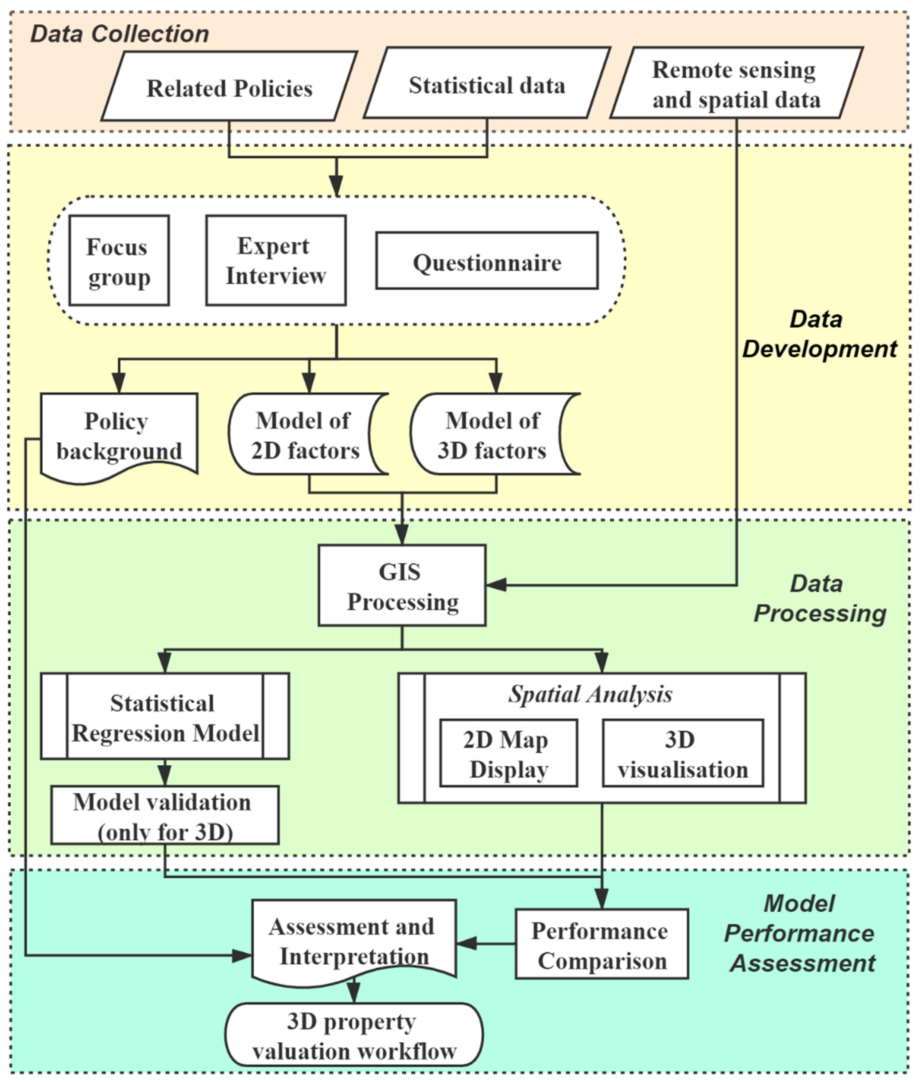
Figure 2.
The study area map. (a) The location of Xi’an; and (b) locations of neighbourhoods Y and Z.
Figure 2.
The study area map. (a) The location of Xi’an; and (b) locations of neighbourhoods Y and Z.
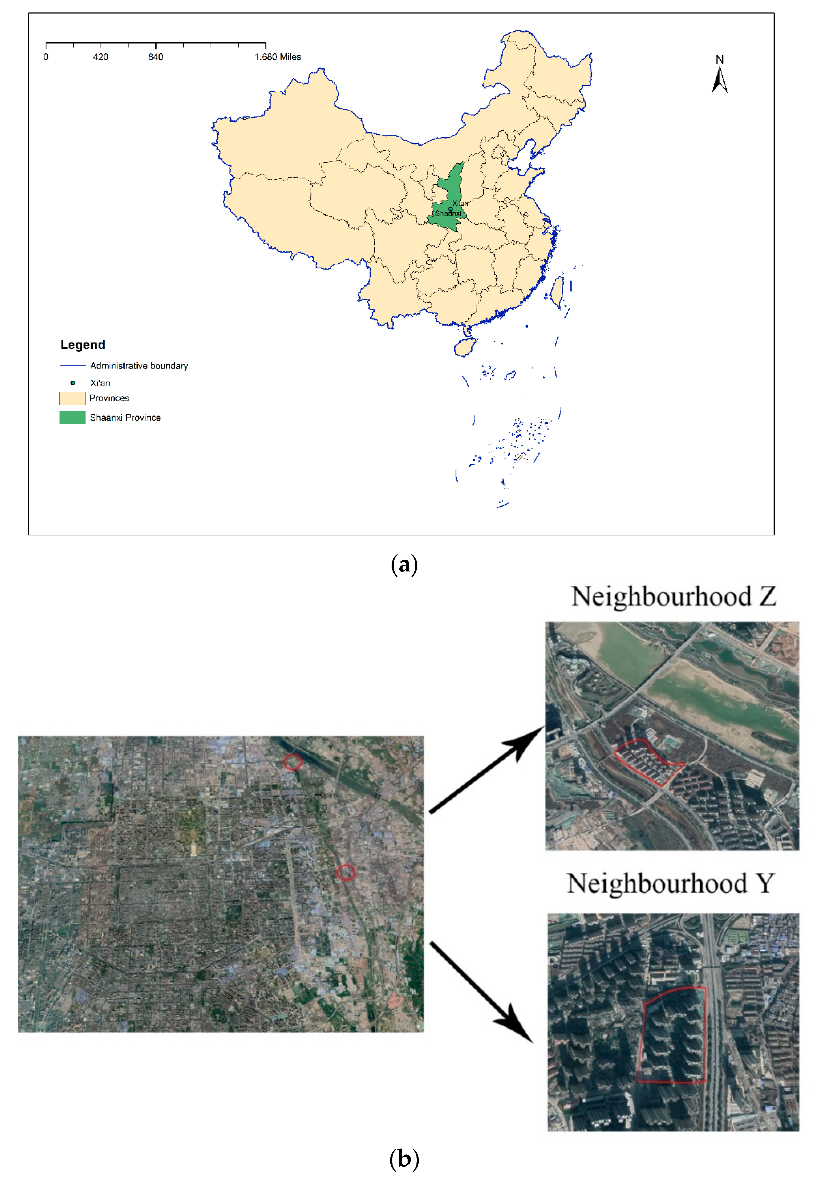
Figure 3.
Workflow for 3D modelling.
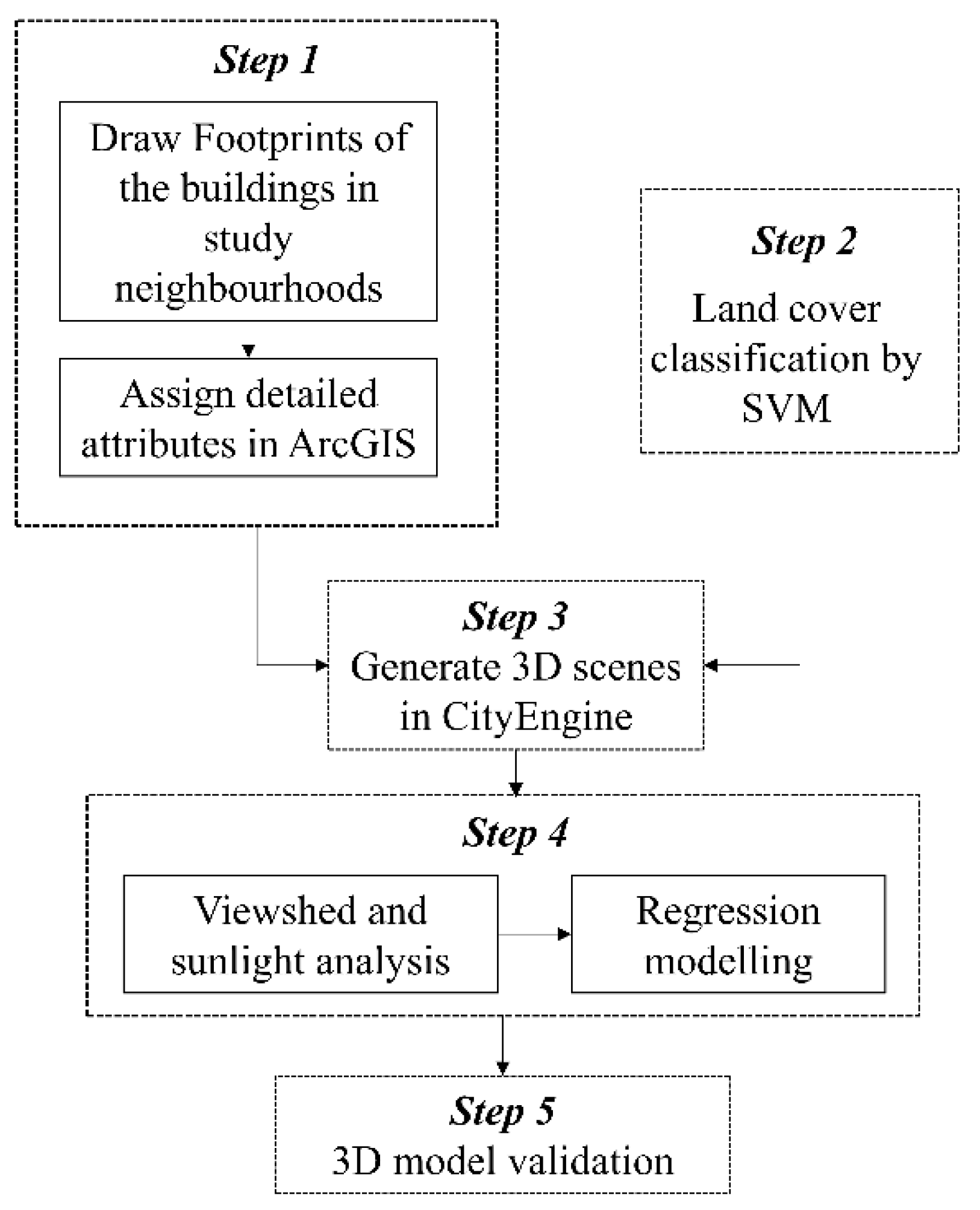
Figure 4.
The maps of local R2 and five significant factors. (a) local R2; (b) density of factory; (c) distance to food; (d) distance to subway; (e) distance to CBD; and (f) NDVI.
Figure 4.
The maps of local R2 and five significant factors. (a) local R2; (b) density of factory; (c) distance to food; (d) distance to subway; (e) distance to CBD; and (f) NDVI.
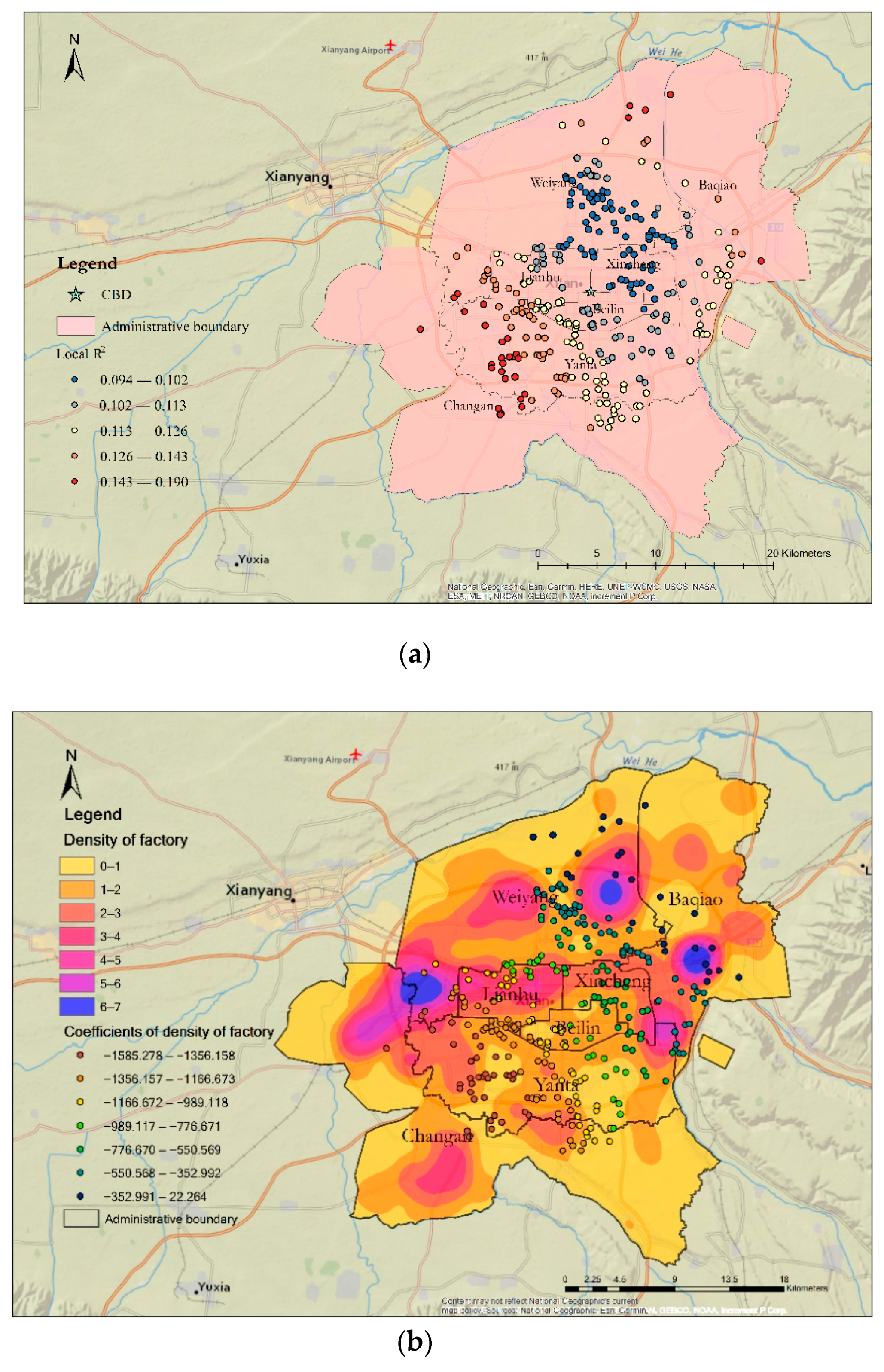
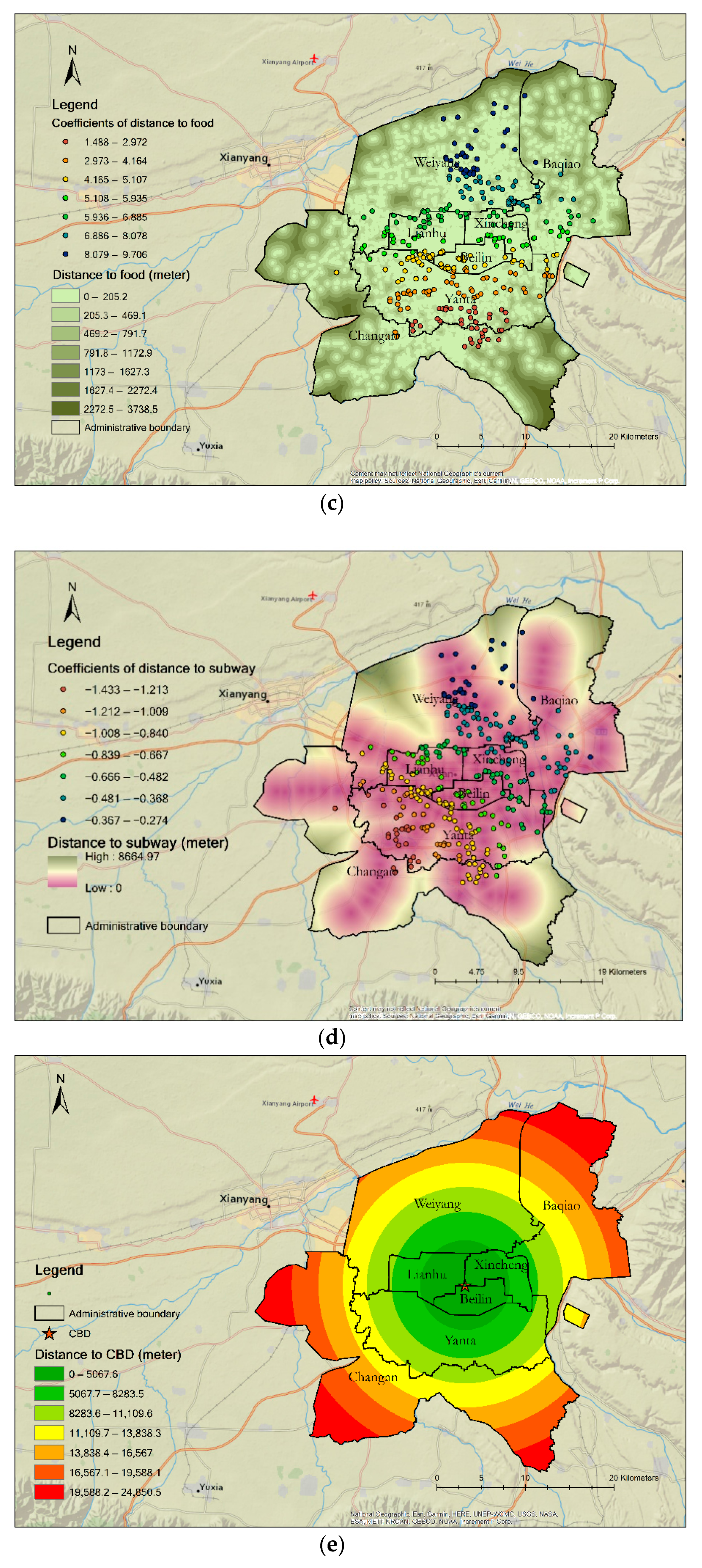
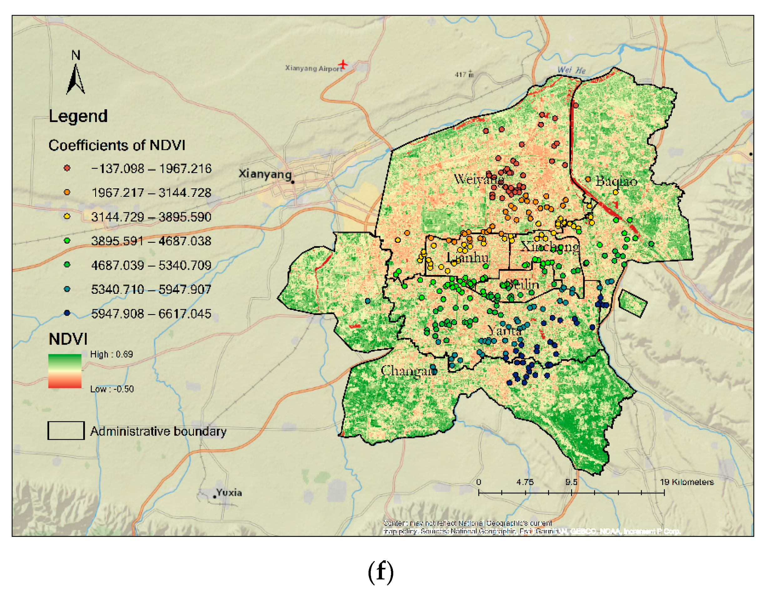
Figure 5.
The 3D analysis of Z as theexample. (a) Helicopter view of Z with building number; (b) detailed screenshots in storey levels; and (c) value variation in different presentations. Since the average value per building is used, one colour is set up per building.
Figure 5.
The 3D analysis of Z as theexample. (a) Helicopter view of Z with building number; (b) detailed screenshots in storey levels; and (c) value variation in different presentations. Since the average value per building is used, one colour is set up per building.
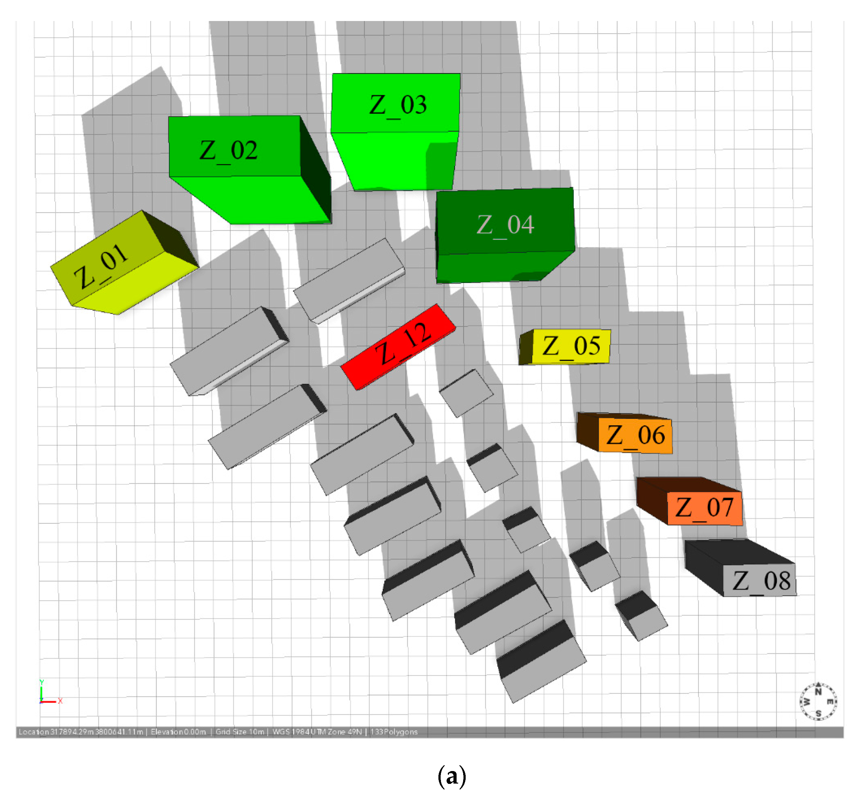
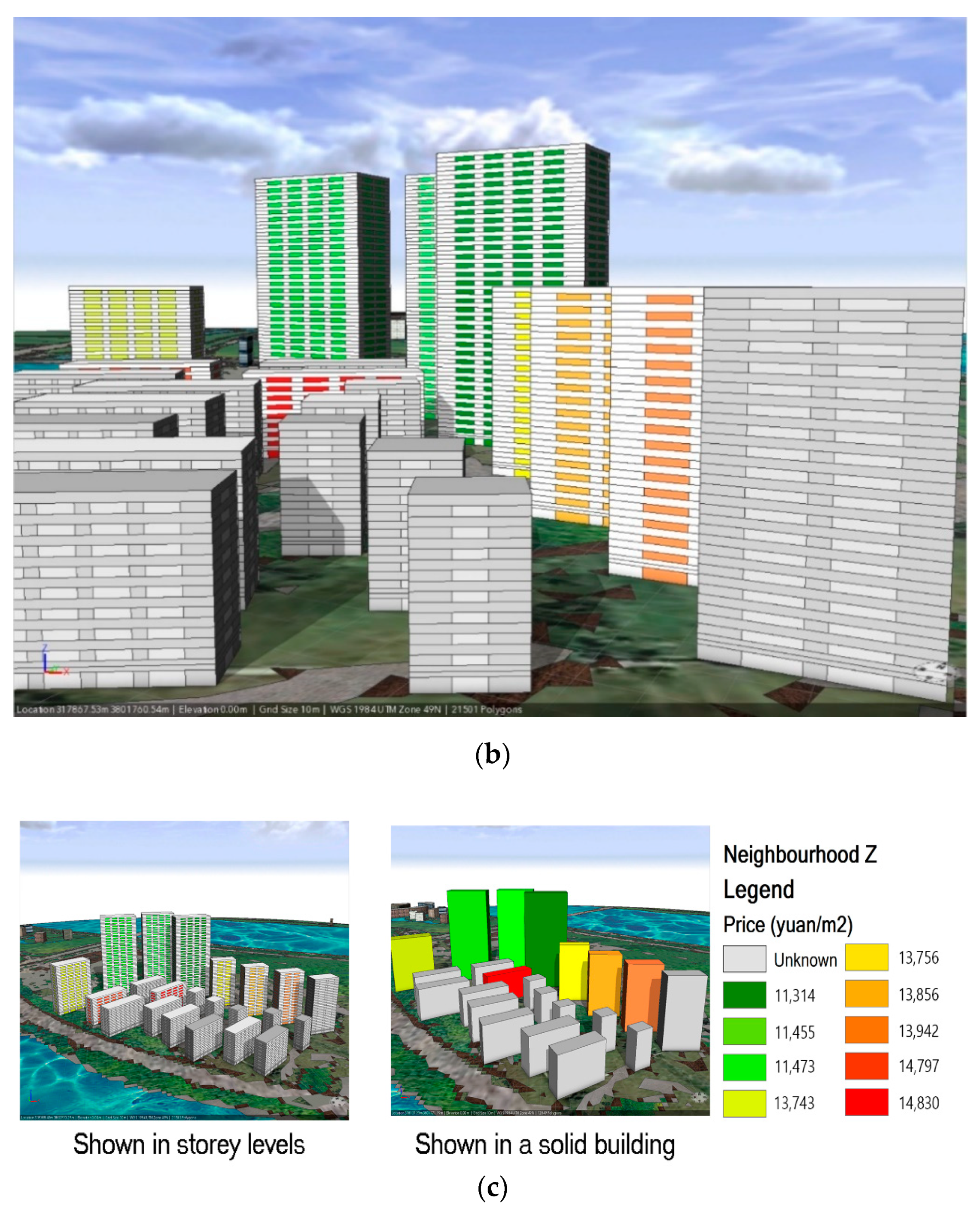
Figure 6.
Diagram of view quality.
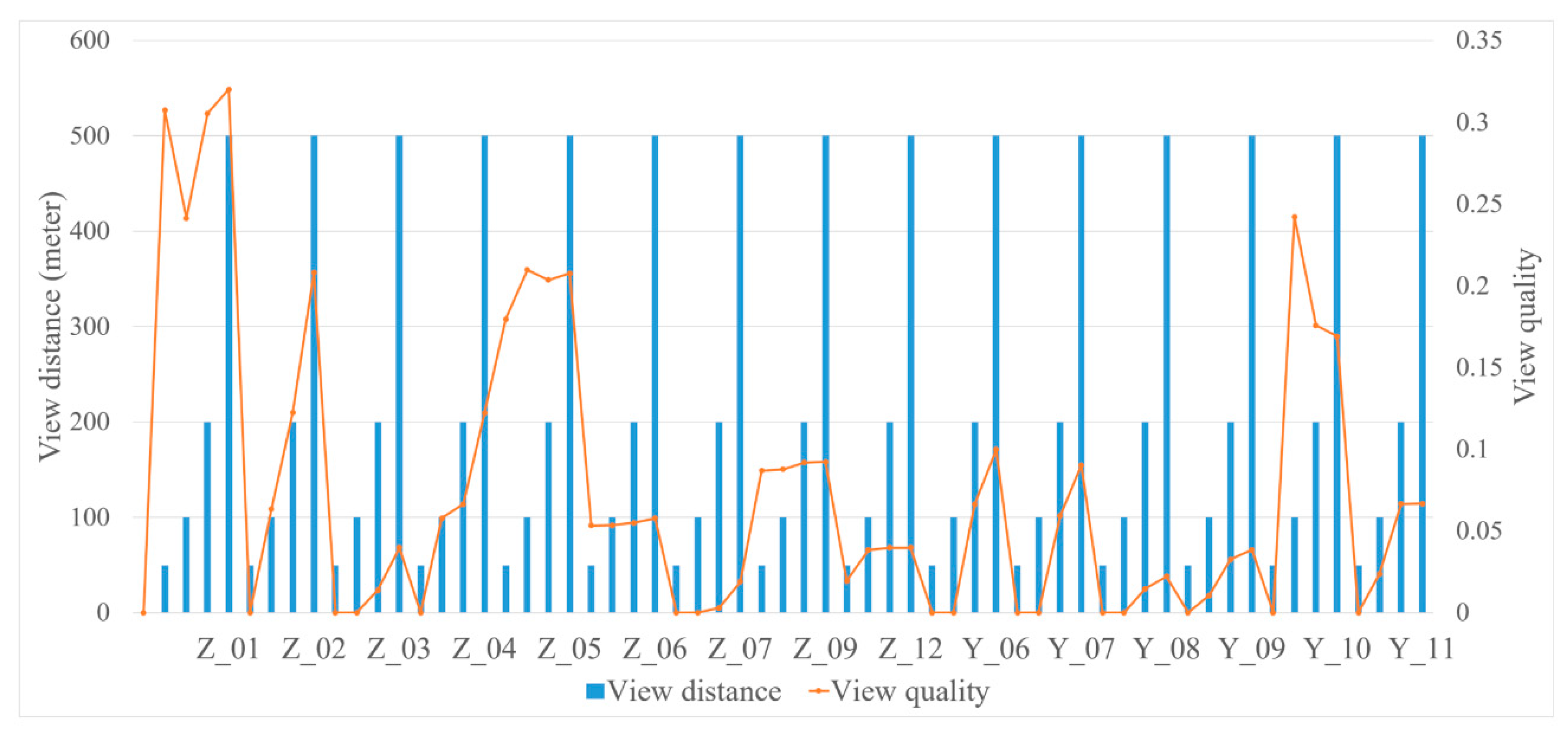
Figure 7.
Diagram of sky view factor (SVF).
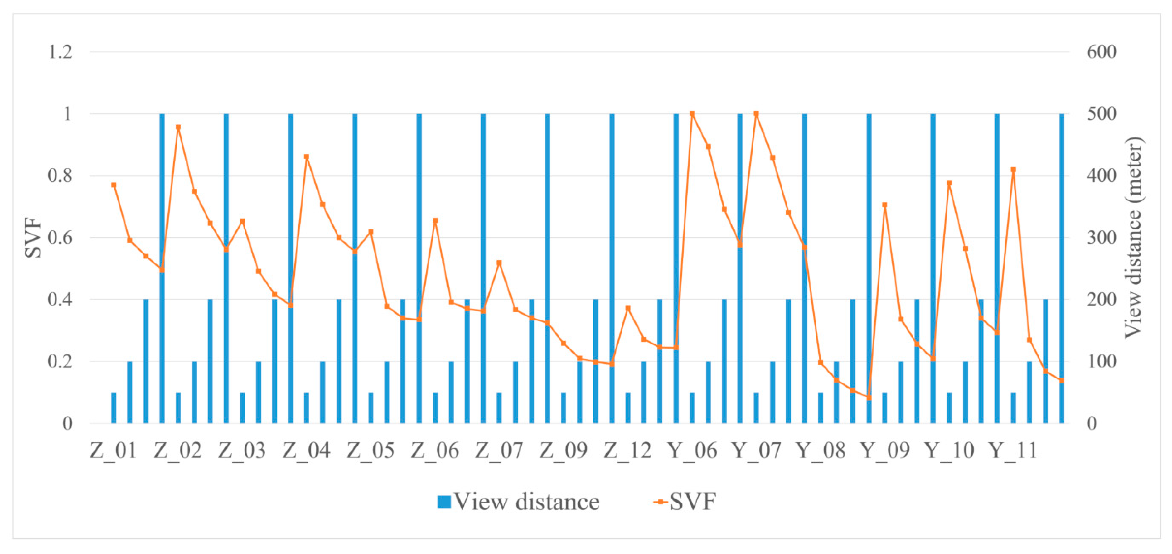
Figure 8.
SVF change of Y_06 and Y_08 under different view distances.
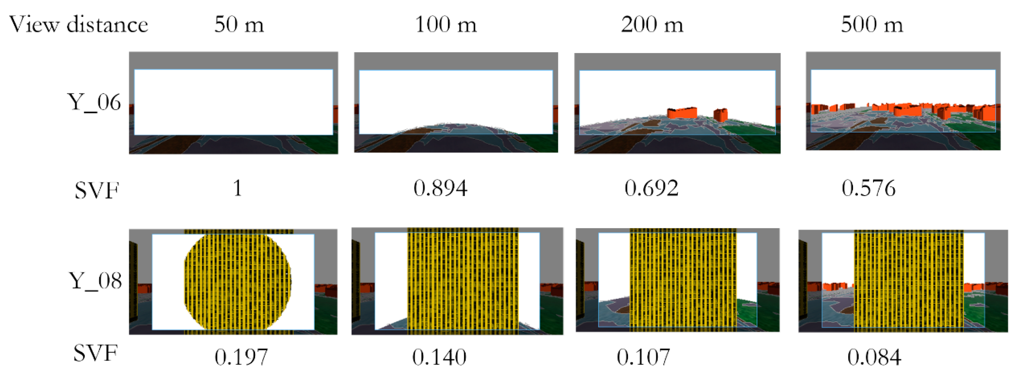
Figure 9.
The comparison of sunlight at different times in a day (Y as an example). The colour indicates the property value (green—low and red—high). Land cover is set to invisible for better visualisation.
Figure 9.
The comparison of sunlight at different times in a day (Y as an example). The colour indicates the property value (green—low and red—high). Land cover is set to invisible for better visualisation.
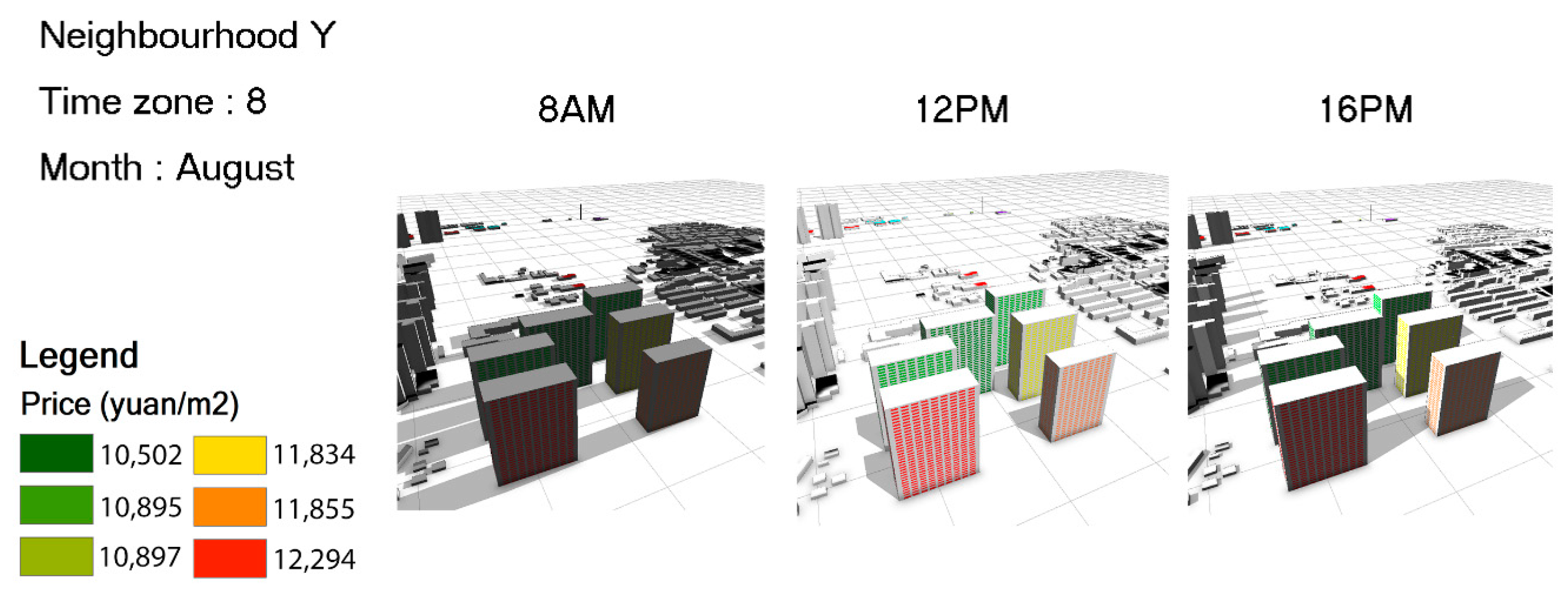
Figure 10.
Leave-one-out cross-validation (LOOCV) results of the 3D model.

Table 1.
Data overview.
| Data | Unit | Source and Description | Purpose |
|---|---|---|---|
| Sentinel-2 satellite image | Tiff | Copernicus Open Access Hub, 10-m resolution, date 26-10-2018, cloud coverage 1.5% | Calculating the normalised difference vegetation index (NDVI). |
| Gaofen-2 satellite image | Tiff | Gaofen-2 Satellite, 4-m resolution, date 12-04-2017, cloud coverage 0.04% | Land cover classification for the 3D model. |
| Google Earth Image | Tiff | Pixel resolution 4800 × 2782, date 24-04-2017 | Land cover classification validation. |
| Floor numbers of the buildings in Xi’an | Vector | Baidu Map and Amap (AutoNavi) | Construct buildings for 3D analyses. |
| Point of interest (POI) of Xi’an | Point | Baidu Map | Creating 2D factors. |
| Footprints of the buildings in neighbourhoods Y and Z | Vector | Google Earth | 3D visualisation and spatial analysis. |
| Database of the average first-hand property values of Xi’an in 2018 | Yuan/m2 | China Index Academy | The dependent variable (regressions) of the 2D model. |
| First-hand property values of the neighbourhoods Y and Z in 2018 | Yuan/m2 | The Price Bureau of Xi’an (http://wjj.xa.gov.cn/) | The dependent variable (regression) of the 3D model. |
Table 2.
Overview of 2D factors.
| Factor | Definition | Unit |
|---|---|---|
| Property value | The first-handed property value of high-rise neighbourhoods. | Yuan/m2 |
| Density of park | The density of the parks within 1 km. | Number |
| NDVI | The mean vegetation inside the neighbourhood within 50 m. | Number |
| Density of factory | The density of the factories within 1 km. | Number |
| Distance to food | Euclidean distance to restaurants, fast-food chains, and eateries. | Meter |
| Distance to college | Euclidean distance to colleges and universities. | Meter |
| Density of hospital | The density of major hospitals within 3 km. | Number |
| Density of supermarket | The density of supermarkets within 1 km. | Number |
| Distance to CBD | Euclidean distance to the central business district (CBD). | Meter |
| Distance to subway | Euclidean distance to subway stations. | Meter |
| Density of bus stop | The density of bus stops within 200 m. | Number |
| Distance to road | Euclidean distance to primary and secondary roads. | Meter |
Table 3.
Overview of 3D factors.
| Factor | Definition | Unit |
|---|---|---|
| View quality | The proportion of the areas of positive view types to the total. | Percentage |
| SVF | The proportion of the visible sky from the observer point [42] | Percentage |
| Sunlight | The proportion of properties with direct sunlight to the total amount of properties at south orientation (per building) | Percentage |
| Property orientation | The preferred orientation of main rooms equals 1; otherwise, it equals 0. | Dummy variable |
Table 4.
Parameter setting for viewshed analysis.
| Parameter | Value | Reference | Description |
|---|---|---|---|
| The horizontal angle of view | 120° | The normal vision range of eyesight. | The horizontal angle of view in a 360° panorama from the observer. |
| The vertical angle of view | 90° | The normal vision range of eyesight. | The vertical angle of view in a 360° panorama from the observer. |
| Observer point of X | / | It changes with the building location. | X coordinate of the observer. |
| Observer point of Y | The middle of the building | It aims to represent the average value. | Y coordinate of the observer. |
| Observer point of Z | / | It changes with the building location. | Z coordinate of the observer. |
| Tilt angle | 0° | The observer looks straight ahead. | Vertical camera view angle. |
| Heading angle | 135° (southeast) or 180° (south) | The orientation from the main rooms. | Horizontal camera view angle. |
| View distance | 50 m, 100 m, 200 m, 500 m | Different view distances contain different view types and areas. | The distance from the observer to the point of interest. |
Table 5.
Descriptive statistics of geographically weighted regression (GWR) estimation coefficients.
Table 5.
Descriptive statistics of geographically weighted regression (GWR) estimation coefficients.
| Variable Name | β Mean | β Min | β Max | β Standardised | β Standard Deviation |
|---|---|---|---|---|---|
| NDVI | 4136.834 | −137.098 | 6617.045 | 2.630 * | 1572.973 |
| Density of bus stop | 2.037 | −26.437 | 21.607 | 0.231 | 8.829 |
| Density of supermarket | −11.377 | −29.688 | 4.423 | −1.441 | 7.896 |
| Density of factory | −870.293 | −1585.278 | 22.264 | −2.171 * | 400.941 |
| Density of hospital | −2880.989 | −5843.088 | 988.861 | −2.221 | 1297.092 |
| Distance to food | 5.455 | 1.488 | 9.706 | 2.695 * | 2.024 |
| Distance to college | 0.104 | −0.435 | 0.984 | 0.341 | 0.305 |
| Distance to road | −1.001 | −2.072 | 0.225 | −1.653 | 0.605 |
| Density of park | −173.801 | −810.403 | 434.060 | −0.680 | 255.686 |
| Distance to subway | −0.701 | −1.433 | −0.274 | −2.304 * | 0.304 |
| Distance to CBD | −0.230 | −0.381 | −0.175 | −4.880 * | 0.047 |
| Local R2 | 0.124 | 0.093 | 0.207 | / | 0.022 |
| Intercept | 11,531.725 | 8847.235 | 14,826.088 | 7.338 | 1571.418 |
| AICc | 5670.436 | ||||
| Adjusted R2 | 0.128 | ||||
* Represents significant at 0.05 level. Bandwidth = 11,834.747.
Table 6.
The results of sunlight analysis.
| Name | Sunlight | Total | Mean | |||||
|---|---|---|---|---|---|---|---|---|
| 8 June (A.M.) | 12 June (A.M.) | 16 June (P.M.) | 8 Dec (A.M.) | 12 Dec (A.M.) | 16 Dec (P.M.) | |||
| Y_06 | 0.000 | 1.000 | 1.000 | 0.000 | 1.000 | 1.000 | 4.000 | 0.667 |
| Y_07 | 0.000 | 1.000 | 1.000 | 0.000 | 1.000 | 1.000 | 4.000 | 0.667 |
| Y_08 | 0.000 | 1.000 | 1.000 | 0.000 | 0.261 | 0.506 | 2.767 | 0.461 |
| Y_09 | 0.000 | 1.000 | 0.977 | 0.000 | 0.443 | 0.773 | 3.193 | 0.532 |
| Y_10 | 0.000 | 1.000 | 1.000 | 0.000 | 0.902 | 0.122 | 3.024 | 0.504 |
| Y_11 | 0.000 | 1.000 | 1.000 | 0.000 | 0.347 | 0.209 | 2.556 | 0.426 |
| Z_01 | 0.833 | 1.000 | 0.000 | 0.431 | 1.000 | 0.000 | 3.264 | 0.544 |
| Z_02 | 0.000 | 1.000 | 1.000 | 0.000 | 0.970 | 1.000 | 3.970 | 0.662 |
| Z_03 | 0.000 | 1.000 | 0.000 | 0.000 | 0.773 | 0.962 | 2.735 | 0.456 |
| Z_04 | 0.000 | 1.000 | 1.000 | 0.000 | 0.909 | 0.848 | 3.758 | 0.626 |
| Z_05 | 0.000 | 1.000 | 1.000 | 0.000 | 0.656 | 0.944 | 3.601 | 0.600 |
| Z_06 | 0.000 | 1.000 | 1.000 | 0.000 | 1.000 | 0.778 | 3.778 | 0.630 |
| Z_07 | 0.000 | 1.000 | 1.000 | 0.000 | 0.563 | 0.806 | 3.368 | 0.561 |
| Z_09 | 0.000 | 1.000 | 0.000 | 0.000 | 0.556 | 0.000 | 1.556 | 0.259 |
| Z_12 | 0.625 | 1.000 | 0.000 | 0.000 | 0.688 | 0.000 | 2.313 | 0.385 |
Table 7.
Descriptive statistics of the 3D model.
| Variable Name | Standardised Coefficient | t-Ratio | p-Value | Tolerance | VIF |
|---|---|---|---|---|---|
| View quality | −0.123 | −1.046 | 0.300 | 0.725 | 1.379 |
| SVF | −0.271 | −2.005 | 0.050 * | 0.547 | 1.828 |
| Property orientation | −0.792 | −5.747 | 0.000 ** | 0.526 | 1.901 |
| Sunlight | 0.327 | 2.000 | 0.050 * | 0.812 | 2.682 |
| Constant | 13,637.143 | 19.028 | / | / | / |
R2 = 0.451, adjusted R2 = 0.411, Durbin–Watson = 0.432, *: significant at the 0.05 significance level; **: significant at the 0.01 significance level.
Table 8.
Comparison of 2D and 3D models.
| Name | R2 | Adjusted R2 | SSR |
|---|---|---|---|
| OLS | 0.111 | 0.077 | 3,392,667,848 |
| GWR | 0.217 | 0.128 | 2,655,158,522 |
| 3D | 0.451 | 0.411 | 125,452,566 |
Publisher’s Note: MDPI stays neutral with regard to jurisdictional claims in published maps and institutional affiliations. |
© 2020 by the authors. Licensee MDPI, Basel, Switzerland. This article is an open access article distributed under the terms and conditions of the Creative Commons Attribution (CC BY) license (http://creativecommons.org/licenses/by/4.0/).
Share and Cite
MDPI and ACS Style
Ying, Y.; Koeva, M.; Kuffer, M.; Asiama, K.O.; Li, X.; Zevenbergen, J. Making the Third Dimension (3D) Explicit in Hedonic Price Modelling: A Case Study of Xi’an, China. Land 2021, 10, 24. https://doi.org/10.3390/land10010024
AMA Style
Ying Y, Koeva M, Kuffer M, Asiama KO, Li X, Zevenbergen J. Making the Third Dimension (3D) Explicit in Hedonic Price Modelling: A Case Study of Xi’an, China. Land. 2021; 10(1):24. https://doi.org/10.3390/land10010024
Chicago/Turabian StyleYing, Yue, Mila Koeva, Monika Kuffer, Kwabena Obeng Asiama, Xia Li, and Jaap Zevenbergen. 2021. "Making the Third Dimension (3D) Explicit in Hedonic Price Modelling: A Case Study of Xi’an, China" Land 10, no. 1: 24. https://doi.org/10.3390/land10010024
Note that from the first issue of 2016, this journal uses article numbers instead of page numbers. See further details here.