1. Introduction
The number of extreme rainfall events has increased drastically during the last two decades [
1]. In addition, the extreme daily rainfall averaged over both dry and wet regimes shows robust increases in both observations and climate models over the six decades [
2]. The global flood cost due to extreme rainfall events has reached a total of USD 470 billion since 1980 [
3]. In addition, 8835 disasters, 1.94 million deaths and USD 2.4 trillion of economic losses were reported globally as a results of droughts, floods, windstorms, etc. from 1970 to 2012 [
4]. Moreover, climate change would likely exacerbate this trend in the near future. The rainfall observations showed a general increase in the heavy or torrential rainfall at a global scale. The results predicted using a General Circulation Model (GCM) indicated an increase in the extreme rainfall associated with global warming [
5]. Saidi et al. [
6] discussed the intensification of heavy-rainfall events due to climate change in Italy.
In particular, climate anomalies have caused more torrential rainfalls and typhoons in South Korea. South Korea has been experiencing unprecedented torrential rainfalls since 1998, e.g., 500 mm/day in the Imjin River basin, 870 mm/day in the Gangwon Province, etc. As the mean annual rainfall that occurred in South Korea was approximately 1300 mm, the rainfall record of 870 mm/day amounts to approximately 65% of the mean annual rainfall. Recently, torrential rainfalls have become one of the most frequent, widespread, severe meteorological hazards affecting South Korea. Moreover, natural hazards associated with torrential rainfalls, such as flash flood, stream flooding, and landslides, occur repeatedly [
7].
The term torrential rainfall refers to rain that is pouring quite heavily. Although there is no formal or scientific definition for torrential rainfall, the Meteorological Administration of South Korea defines the rainfall to be torrential if the amount of rainfall is higher than 80 mm/day or 30 mm/h because these rainfall intensities usually occur abrupt landslides. Hence, in this study, torrential rainfall was defined as the amount of rainfall that is higher than 80 mm/day because only daily rainfall data were collected. The magnitude of extreme rainfall at a specific return period by the rainfall frequency analysis is very important because it is used as a reasonable design value for various hydraulic structures such as levees, dams, etc. Meanwhile, the statistical characteristics of the number of torrential rainfall occurrences are very important because it should be used for structural or nonstructural measure to prevent flood in a given region of interest. Hence, the objective of this study is to develop a methodology considering the statistical characteristics of the frequency distribution to fit the number of torrential rainfall occurrences.
Many researchers modeled rainfall to understand flood, drought, and environmental processes effectively. A stochastic model of precipitation that relates to the number of storms in a given time interval was reported by Todorovic and Yevjevich [
8]. They used the Poisson distribution to represent the random properties of the rainfall process. Markov chain models were developed to represent the sequence of rainfall series [
9,
10,
11,
12]. Instead of Markov chains, some studies used various probability distributions. The gamma distribution containing two parameters was often used in fitting the rainfall amount [
13,
14,
15]. Other probability distributions such as exponential, mixed exponential, and Weibull distributions were employed in the analysis of rainfall characteristics [
16,
17]. Nourani et al. [
18] used a multivariate ANN-wavelet technique to develop a rainfall–runoff model. Recently, Rauf and Zeephongsekul [
19] suggested nonparametric copulas to analyze the rainfall severity and duration in Australia.
One of the difficulties of employing probability distributions to model rainfall events is that the data pertaining to rainfall events are continuous consisting of exact zeros. Hence, it is difficult for most statistical models to analyze events consisting of both discrete and continuous distributions [
20]. As this study focuses on the number of torrential rainfall occurrences, the data, namely, count data, can be modeled using the discrete probability distributions. For applications of count data, the Poisson distribution has been widely used to represent their statistical properties. However, it was reported that the Poisson distribution often underestimated or overestimated the observed dispersion because of additional or fewer zeros. Cohen [
21] and Lambert [
22] showed that this phenomenon might have occurred because a parameter in the Poisson distribution (POI) was often insufficient to describe the same population. They suggested that the general Poisson distribution (GPD) could not fit the count data having additional zeros. Therefore, they proposed the Zero-Inflated Poisson (ZIP) model to solve the problem caused by additional or fewer zeros. After the development of the ZIP model, Gupta et al. [
23] proposed the Zero-Inflated Generalized Poisson (ZIGP) model. They estimated three parameters in the ZIGP model using the Maximum Likelihood Estimation (MLE) method and provided the asymptotic variance–covariance of the estimators. In particular, Angers and Biswas [
24] proposed the Bayesian framework for the ZIGP model and showed the appropriate priors and posteriors using the Monte Carlo integration via importance sampling.
The applications of the ZIP and ZIGP models for the count data were reported in scientific areas such as sociology, engineering, and agriculture. However, in the field of water-related studies, the application of the zero-inflated concept is quite limited. Silva et al. [
25] used the ZIP model to perform flood frequency analysis via the peaks-over-threshold method.
In this study, the five different models, POI, GPD, ZIP, ZIGP, and Bayesian ZIGP were developed and applied to the torrential rainfall data obtained from the two rain gauges in South Korea. In particular, in the procedure of the Bayesian framework, the informative prior distributions were evaluated to provide more accurate results.
2. Models for Zero-Inflated Count Data
2.1. Zero-Inflated Poisson (ZIP) Model
Poisson distribution has been frequently used to model the count data [
26,
27]. However, one often encounters count data where the number of zeros is such that the Poisson distribution cannot fit the data. Bohning et al. [
28] showed clearly this phenomenon using DMFT (Decayed, Missing and Filled Teeth) data. Johnson et al. [
29] suggested that zero-inflated concept could be used to resolve this problem. Consider a discrete random variable,
with mass concentrated on the integers. If
is observed with frequency higher or lower than that predicted theoretically by the assumed model, then the adjusted random variable
can be described as following equation.
where
is a weighting parameter. Thus, in the case
, this adjusted model can incorporate extra zeros and, in the case
, this model can deal with fewer zeros than given by the original model (
). This adjusted model is called as “ZIP model” when the Poisson distribution,
is used in Equation (1). Thus, ZIP model can be described as Equation (2). In addition, the two parameters in ZIP model,
and
, can be estimated simply by the method of moments as Equation (3).
where
and
are the variance and mean of the sample data, respectively.
2.2. Zero-Inflated Generalized Poisson (ZIGP) Model
Consul and Jain [
30] suggested the form of GPD with two parameters. This GPD provides a very close fit to supposedly binomial, Poisson, and negative binomial data. Consul and Jain [
30] showed this phenomenon accurately through the analysis using various data such as industrial accidents, spatial distribution of insects, etc. Equation (4) is the probability mass function of the GPD and Equation (5) is the estimates to the two parameters by the method of moments. Especially, the conditions for
and
should be satisfied as
and
.
The GPD developed by Consul and Jain [
30] can also be applied to zero-inflated model to resolve the problem from extra zeros or fewer zeros. The zero-inflated model with GPD is called as ZIGP model and this model can be represented by Equation (6).
where the parameter
having range
controls the form of ZIGP model. When
is zero, then ZIGP model reduces to ZIP model. In ZIGP model, we have inflated zeros in the case of
and also if
. The three parameters in ZIGP model can be estimated by MLE method.
Angers and Biswas [
24] described the estimates by MLE to develop Bayesian ZIGP model. Let
be the number of times
takes the value
and suppose we have
sample observations in total. By mathematical manipulation with
and
, the likelihood function of ZIGP model can be described as Equation (7). In this procedure, the objective is to maximize likelihood function to the given data. This is performed by taking the three partial derivatives of likelihood function and equating them to zero. The resulting set of equations is then solved simultaneously to obtain the estimates to the three parameters,
.
2.3. Bayesian Zero-Inflated Generalized Poisson (Bayesian ZIGP) Model
2.3.1. Framework of the Bayesian ZIGP Model
The estimation of the number of torrential rainfall events using the Bayesian framework is very useful because this approach incorporates various information, such as statistical data or expert judgment, and it can be used appropriately when the size of the collected data is small. However, the computing power required to solve a posterior distribution was insufficient, thereby limiting the application of the framework during the 1970s and 1980s. After the 1980s, the growing computing capacity and algorithms enabled the application of the Bayesian framework. Malakoff [
31] mentioned that a 236-year-old approach to statistics was making a comeback as it has the ability to factor in hunches as well as hard data applications from pharmaceuticals to fisheries. Hence, recently, the Bayesian approach has been widely used in the fields of science and engineering. In the planning and management of water resources, such as flood or low-flow frequency analysis, regional analysis, and calibration of rainfall–runoff models, several studies that incorporated the Bayesian approach were conducted [
32,
33,
34,
35,
36,
37,
38].
Despite numerous applications of the Bayesian approach, relatively fewer studies regarding the development of the Bayesian framework using the ZIP or ZIGP model were conducted. Angers and Biswas [
24] employed a noninformative prior distribution and developed a posterior distribution for the ZIGP model. In addition, they applied the importance sampling, which is a technique used in the Monte Carlo integration, and argued that the classical statistical inference procedures, such as the method of moment and MLE, were not always suitable to make inferences of the parameters in the ZIP or ZIGP model. Ghosh et al. [
39] performed the Bayesian analysis for the ZIP regression model. They employed the Bayesian estimation method using conjugate priors and performed the Gibbs sampling technique to obtain a large number of random variates from a posterior distribution. In particular, they suggested that the Bayesian framework outperformed the classical estimation method, such as MLE, in terms of both bias and precision.
The Bayesian approach is based on specifying a probability model for the observed data
and a vector
of unknown parameters. Given the observed data
, the Bayes’ theorem can be used to determine the posterior distribution of
via the following equation.
where
is a posterior distribution,
is a likelihood function,
is a prior distribution, and the denominator of the RHS (Right Hand Side) is a normalizing constant. In addition,
is
in Equation (7).
2.3.2. Elicitation of Prior Distribution
The most important and controversial step in developing the Bayesian framework is the selection of a prior distribution, which represents the information of an uncertain parameter. Generally, two types of prior distributions can be used to perform the Bayesian Markov Chain Monte Carlo (MCMC) scheme using the Metropolis–Hastings algorithm. One is the noninformative prior distribution, such as the conjugated distribution, and the other is the informative prior distribution using the empirical Bayes method. If large amounts of data are available, noninformative prior distribution can be useful. Many studies used the noninformative prior distribution [
40,
41,
42]. As an informative prior distribution uses the analyst’s beliefs regarding unknown parameters, it is contrary to the mathematical definition of the noninformative prior distribution. However, if the sample size is small or the available data only provide indirect information, the development of an informative prior distribution becomes more useful [
34,
38]. As previously mentioned, the two-stage Bayes method [
43], the empirical Bayes method [
34,
38,
44,
45], and the maximum entropy method [
46] were used to elicit an informative prior distribution. Among the methods, the empirical Bayes method was used in this study because it was the commonly used procedure, which enabled the use of the auxiliary empirical data from some observations of the related parameters. In the empirical Bayes method, the unknown parameters in the prior distribution should be estimated using the MLE method by collecting the available data.
As the likelihood function for the ZIGP model was already described (Equation (7)), the prior distribution for the three parameters in the ZIGP model can be elicited. Angers and Biswas [
24] used two uniform distributions and the Jeffreys’ prior distribution for the Poisson distribution. However, the informative distributions using the empirical Bayes method were elicited in this study for more realistic results. The detailed procedure for the elicitation of the informative prior distribution by empirical Bayes method is described in
Section 4.
2.3.3. Metropolis–Hastings Algorithms and Choice of Proposal Distribution
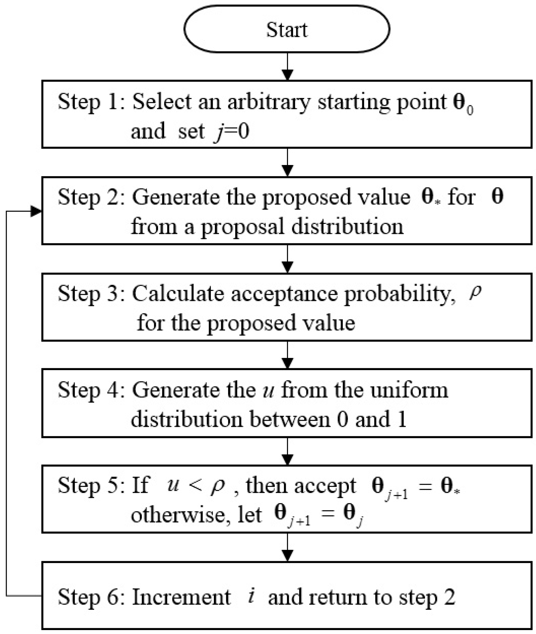
Equation (8) cannot be solved directly, as the prior and the posterior are not conjugate family. In this case, numerical methods, such as the Gibbs sampling or Metropolis–Hastings algorithm based on the Bayesian MCMC scheme, should be used to sample the data from the posterior distribution.
The Metropolis–Hastings algorithm [
47] is the one of most popular algorithm for obtaining a sequence of random samples from a probability distribution for which direct sampling is difficult [
48,
49,
50]. This algorithm simulates the Markov chains in the Monte Carlo integration to generate a set of samples whose distribution converges to a posterior distribution. The Metropolis–Hastings algorithm works by generating a sequence of values in such a way that the distribution of the values more closely approximates the desired distribution. These sample values are produced iteratively with the distribution of the next sample being dependent only on the current sample value. After the iterative sampling process, this algorithm selects a candidate for the next sample value based on the current sample value. Finally, the candidate is either accepted or rejected using the acceptance probability. Hence, the reasonable acceptance probability is most important to draw the desirable random samples. The acceptance probability can be expressed using Equation (9).
where
is the acceptance probability, which is less than 1. Moreover,
is a target distribution, and
is a proposal distribution.
Figure 1 shows the procedure of the Metropolis–Hastings algorithm for the sampling from a posterior distribution.
In these steps, the selection of the proposal distribution is crucial for obtaining the reasonable acceptance rate (or acceptance probability). Roberts et al. [
51] proposed that the acceptance rate should be approximately 45%. Gamerman [
52] indicated that the acceptance rate should be in the range 20%–50%. In particular, the statistical properties of the Markov chain strongly depend on the selected proposal distribution and its parameters. Chib and Greenberg [
49] concluded that the adequate proposal distributions can be selected from the five types of distributions that require the specification of such tuning parameters, such as the shape and the scale. If some selected proposal distribution shows poor mixing in the results, other distributions should be searched to improve the simulated results.
In addition, the tuning of parameters in the selected proposal distribution is important to generate well mixed results. There are two types of approaches: manual tuning through trial-and-error and automatic tuning through some optimization techniques. The automatic tuning approach is called as adaptive MCMC. In the case of the high dimensions, the adaptive MCMC, which asks the computer automatically, can be used. This adaptive MCMC scheme has been applied in a variety of studies [
53,
54,
55]. However, if the dimensions of parameters are low, the tuning of parameters in the selected proposal distribution can be performed by manual tuning.
In this study, a normal distribution
suggested by Metropolis et al. [
47] was selected as the proposal distribution. In addition, a manual tuning method was used because the number of parameters was only one per the three parameters,
, and the adaptive MCMC methods was too difficult.
The selected proposal distribution was very useful in the manipulation of the acceptance probability because of the symmetry of the distribution. Note that when the selected proposal distribution such as is symmetric, and become the same. Therefore, the calculation of the acceptance probability, becomes simple.
The most important step to perform Metropolis–Hastings algorithm is to check the convergence of the developed algorithm. Especially, the important issue is choosing
in the proposal distribution. If
is very small, the almost proposed estimates will be accepted, but they will represent very small movements, and finally, the chain will not mix well. In addition, if
is too large, the almost proposed estimates will be rejected and the chain will not move at all. Although the Metropolis–Hastings algorithm has incorporated an enormous expansion of the classical statistical models, problems exist pertaining to the convergence of simulation results [
56]. When there is no convergence in the results, the draws may be unrepresentative of the whole support the specific distribution and finally leads to poor inference. Lee et al. [
38] used the trace plot and three quantitative diagnostics by Gelman and Rubin [
57], Raftery and Lewis [
58], and Geweke [
59] to check the convergence of the developed Metropolis–Hasting algorithm. Lee et al. [
38] developed the codes for these diagnostics by Matlab software (MathWorks, Natick, MA, USA). Therefore, these codes were used to check the convergence of the algorithm in this study.
2.3.4. Gelman and Rubin’s Diagnostic
Based on normal theory approximation to exact Bayesian posterior inference, the Gelman and Rubin’s diagnostic [
57] is performed with the following steps:
Run chains of length from over-dispersed starting values.
Discard the first draws in each chain.
Calculate the within-chain variance (W) and between-chain variance (B).
Calculate the estimated variance of the parameter as a weighted sum of the within-chain and between-chain variance.
Convergence is monitored by estimating the factor by which the scale parameter might shrink if sampling were continued indefinitely as Equation (10):
where
B is the variance between the means from the
m parallel chains,
W is the average of the
m within-chain variances, and
df is the degrees of freedom of the approximating
t density. In this method, convergence can be evaluated by examining the proximity of shrink factor,
to 1. In addition, it is noted that a higher level of precision may be required in this diagnostic.
2.3.5. Raftery and Lewis’s Diagnostic
Raftery and Lewis’s diagnostic [
58] to detect convergence to the stationary distribution and to provide a way of bounding the variance of estimates of quantile of functions of parameters was used. Suppose the user wants to measure some posterior quantile of interest
q. If the user defines some acceptable tolerance
r for
q and a probability
s of being within that tolerance, the Raftery–Lewis diagnostic can calculate the number of iterations
N and the number of burn-in
M necessary to satisfy the stationary conditions. The Raftery–Lewis diagnostic is performed with following steps:
Select a posterior quantile of interest q.
Select an acceptable tolerance r for this quantile.
Select a probability s, which is the desired probability of being within (q − r, q + r).
Run a pilot sampler to generate a Markov chain with minimum length using the inverse of the normal cumulative distribution function.
Calculate the dependence factor, I. This factor can be interpreted as the proportional increase in the number of iterations attributable to serial dependence. Especially, high dependence factor (>5) means the mixing of chain is poor.
2.3.6. Geweke’s Diagnostic
Geweke [
59] developed the diagnostic that compares the location of the sampled parameter on two different time intervals. If the mean values of the parameter in the two time intervals are somewhat close to each other, it is assumed that the two different parts of the chain have similar locations in the state space. Thus, it is assumed that the two samples come from the same distribution. Let us consider the sample parameters on two different time intervals such as
and
(
and
). In this case, the means for the two different time periods,
and
can be calculated by Equation (11).
If the chain has converged at time
n0, then the two means
and
should be equal and Geweke’s statistic has an asymptotically standard normal distribution as Equation (12).
where
and
are spectral density in two different time periods. Therefore, the null hypothesis of equal location is rejected if
is larger than critical value under the specific confidence level and this finally indicates that the chain has not yet converged by time,
n0. Practically, first step is to calculate the test statistic,
Z to the whole chain. If the test statistic is outside the 95% confidence interval, then calculate the test statistic again after discarding 10%, 20%, 30%, and 40%. If the test statistic is still outside 95% confidence interval for the last test, then the chain is considered as failed to converge.
3. Study Area and Data Characteristics
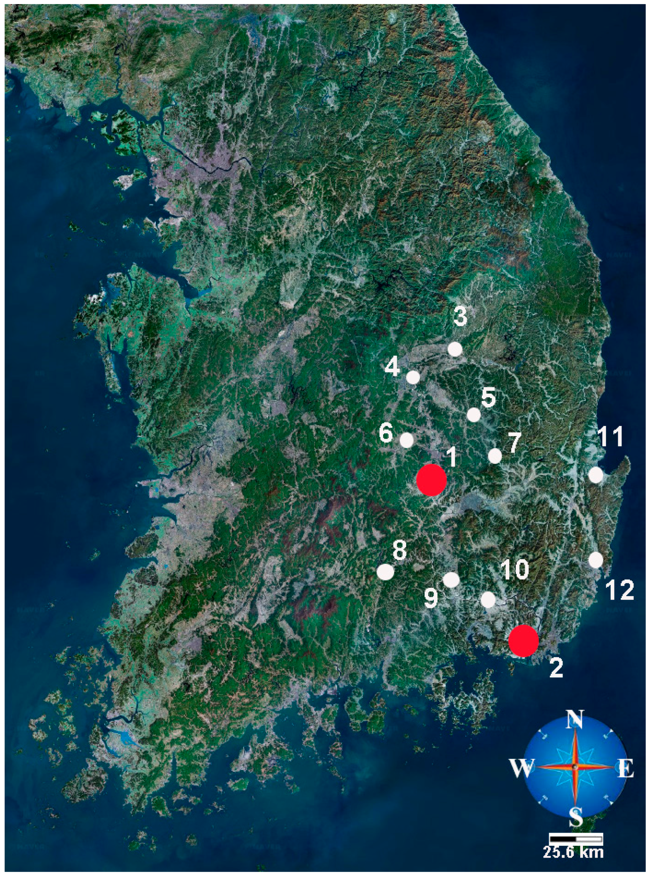
In this study, the statistical properties of the number of torrential rainfall occurrences at the Daegu and the Busan rain gauges in South Korea were analyzed to apply and compare the developed models such as POI, GPD, ZIP, ZIGP, and Bayesian ZIGP. The collected data lengths at two gauges were 32 years (1983–2014). Although the recent 30 years (e.g., 1981–2010) should be used to perform the statistical analysis, 32 years (1983–2014) were used because the starting year of Daegu rainfall gauge was 1983. Daegu is the third largest city after Seoul and Busan in South Korea. Busan is the second largest city located in the southeastern region of the Korean peninsula. Hence, it is important to analyze the statistical property of the occurrences of torrential rainfall to prevent disasters, such as urban flood, in the two cities. Especially, the additional rainfall data were selected from 10 rain gauges (Yeongju, Mungyeong, Uiseong, Gumi, Yeongcheon, Geochang, Hapcheon, Miryang, Pohang, and Ulsan) to elicit an informative prior distribution using the empirical Bayes method.
Figure 2 shows the location of the two target rain gauges (red colored) and the 10 additional rain gauges (white colored).
Table 1 lists the detailed information of the 12 rain gauges and the descriptive statistics of the rainfall data during the 32 years (1983–2014). In addition,
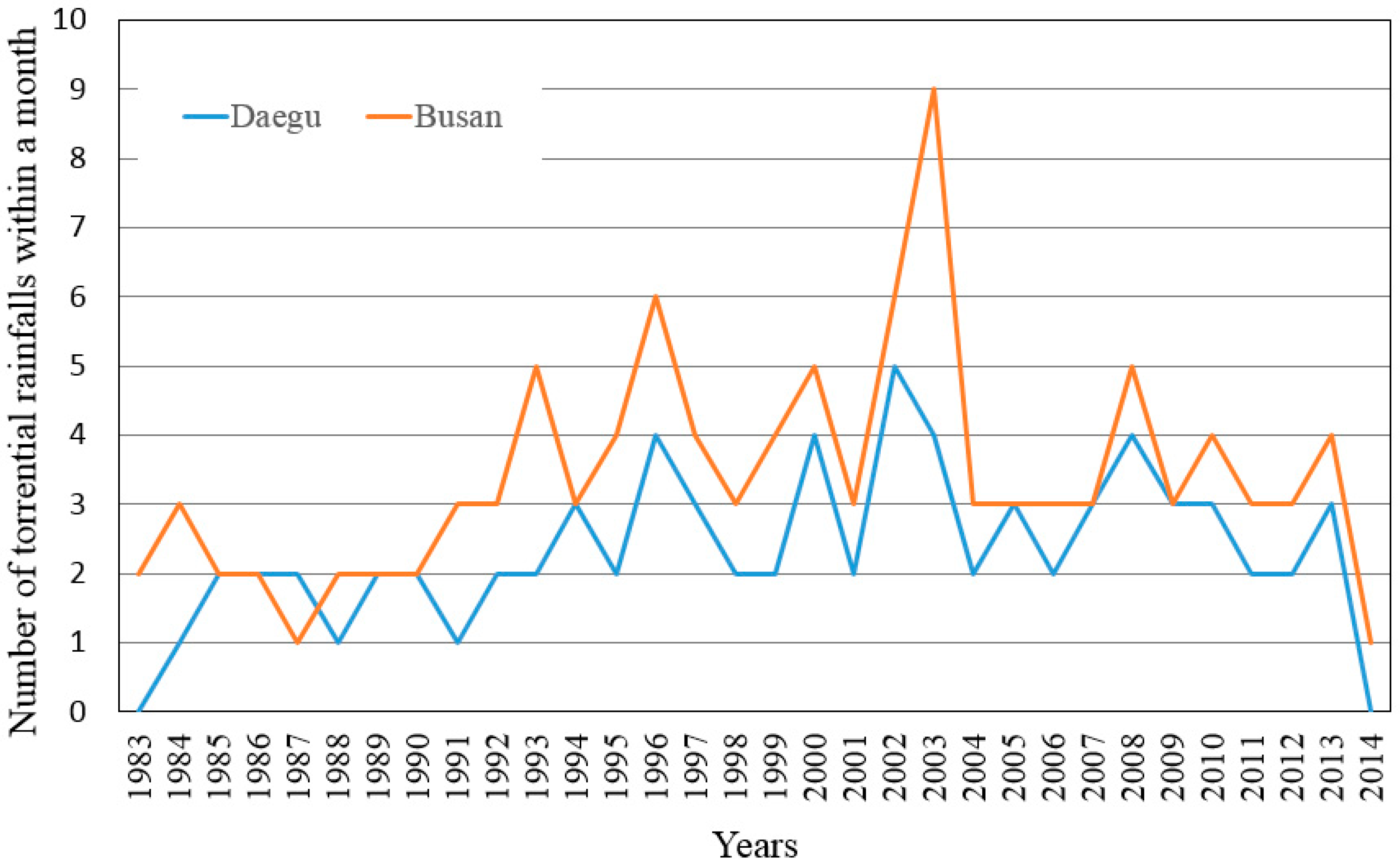
Figure 3 shows the trend of the number of torrential rainfall events within a month at the Daegu and the Busan rain gauges. In
Figure 3, it is suggested that the number of torrential rainfall events within a month were increased after 1994 and 1993 at the Daegu and the Busan rain gauges, respectively.
Table 1, column 6 represents the number of months when the torrential rainfall occurred more than once during a month. In addition,
Table 2 gives the frequency distributions for the torrential rainfall occurrences for the 12 rain gauges. The numbers of torrential rainfall events within a month were 0–6 because the maximum number of torrential rainfall occurrence within a month was 6 in the collected rainfall data. In
Table 1, the highest number (129) of torrential rainfalls for the 384 months occurred at the Geochang rain gauge and the lowest number (56) of torrential rainfalls occurred at the Yeongcheon rain gauge. Moreover, in
Table 2, the highest number of zeros (328) occurred at the Yeongcheon rain gauge and the lowest number of zeros (255) occurred at the Geochang rain gauge. In particular, at the Busan, Yeongju, Mungyeong, Gumi, Geochang, Miryang, and Pohang rain gauges, more than six torrential rainfalls occurred during a given month in the 384 months.
4. Discussion
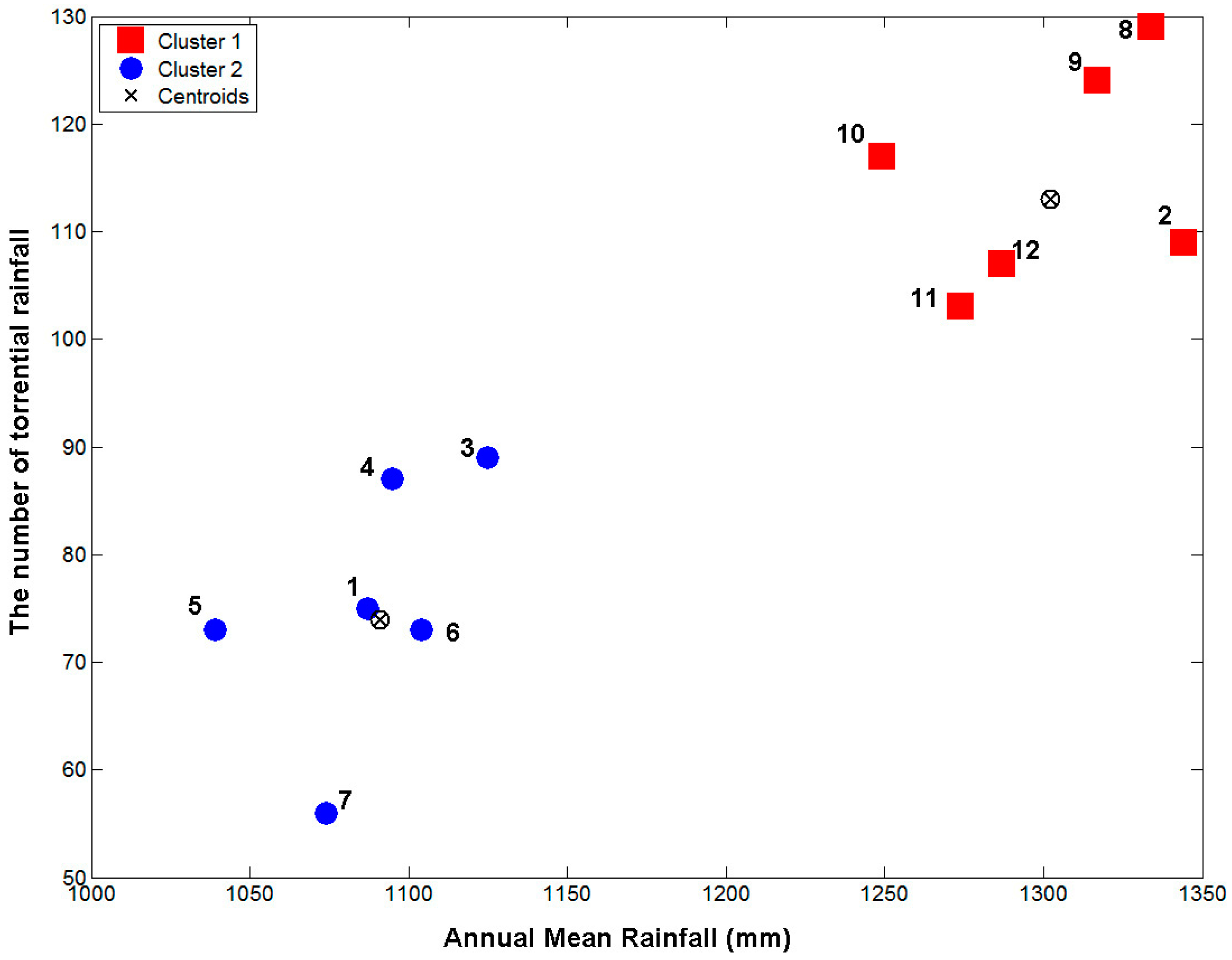
Before the elicitation of an informative prior distribution by empirical Bayes method, the homogeneity of the selected rain gauges should be checked. The cluster analysis can be used to identify the homogenous group. Goyal and Gupta [
60] identified homogenous rainfall regimes in the Northeast region of India using the fuzzy cluster analysis. When the data sets of the rainfall from a specific gauge are homogeneous to the rainfall datasets from other gauges, the data from the other gauges can be used to elicit the prior distribution under ergodic assumption. The ergodic assumption means that time average of a time series is the same as its spatial average. In this study, the cluster analysis using Matlab (Matrix laboratory, R2010a, MathWorks) was performed. Matlab cluster toolbox provides the two types of cluster analysis methods, K-means and hierarchical clustering. Among these, only K-means clustering was performed to group the homogeneous gauges. The objective of the cluster analysis is to find the linear combinations of a set of variables such that a few components that describe most of the variability of the original set are obtained. In this study, the annual mean rainfall and the number of torrential rainfalls at 12 rain gauges, given in
Table 1, were used as variables for the cluster analysis. Although the location or elevation information can be used as another variables for cluster analysis, these variables were excluded in the cluster analysis because the homogeneity on the annual mean rainfall and the number of torrential rainfalls was important to elicit the informative prior distribution.
Figure 4 shows the results of the clustering analysis using the k-means algorithm. Among the 12 rain gauges, Daegu, Yeongju, Mungyeong, Uiseong, Gumi, and Yeongcheon rain gauges were considered one group and Busan, Geochang, Hapcheon, Miryang, Pohang, and Ulsan rain gauges were considered the other.
After the grouping process using the cluster analysis, the empirical Bayes method was applied. The empirical Bayes method uses the classical techniques to fit the prior distribution to the available data from the two groups. Although this procedure is not a pure Bayesian method from a philosophical viewpoint of Bayesian analysis, it can be a pragmatic approach for the elicitation of an informative prior distribution. First, the three parameters,
, of the ZIGP model should be estimated using the classical estimation method MLE for the number of torrential rainfall data, given in
Table 2.
Table 3 gives the estimated results to the three parameters for the 12 rain gauges.
The most suitable probability distribution should be selected for the elicitation of an informative prior distribution after performing the parameter estimation on each data set. To select a suitable probability distribution, four statistical tests,
test, Kolmogorov–Smirnov (K-S) test, Cramer Von Mises test (CVM test), and Probability Plot Correlation Coefficient test (PPCC test), were used in this study. For more detailed theory to these tests, refer to [
61]. When the test values in
test, K-S test, and CVM test are smaller than the table values, the probability distribution can be used. In addition, in PPCC test, when the calculated values are larger than the table value, the probability distribution can be used. The used significance levels in all tests in this study were 5%. These tests were coded by Matlab software (MathWorks).
Table 4 and
Table 5 give the results of the four statistical tests for the three probability distributions: two-parameter Log Normal distribution (LN2), Generalized Extreme Value distribution (GEV), and two-parameter Weibull distribution (WBU2). In this selection, the PPCC test provided the critical clue. Finally,
Table 6 gives the summary of the informative prior distributions and the hyper-parameter values, which were estimated using MLE. In
Table 6, the hyper-parameters 1 and 2 were the estimated parameter of the LN2 (mean and standard deviation) or WBU2 (scale and shape), and the superscript on each parameter represents groups 1 and 2. Finally, the informative prior distribution for the Bayesian ZIGP model was represented under the assumption of the three parameters in ZIGP model, which were independent of each other. Hence, Equations (13) and (14) were developed as the final informative prior distributions in the Bayesian ZIGP model for the groups 1 and 2.
As the likelihood function and prior distributions of groups 1 and 2 were completely developed, the three estimated parameters could be sampled from the posterior distribution in the Bayesian ZIGP model. To do this sampling, Metropolis–Hastings algorithm was employed because the posterior distribution in Equation (8) was quite complex.
5. Performance of the Metropolis–Hastings Algorithm and Convergence
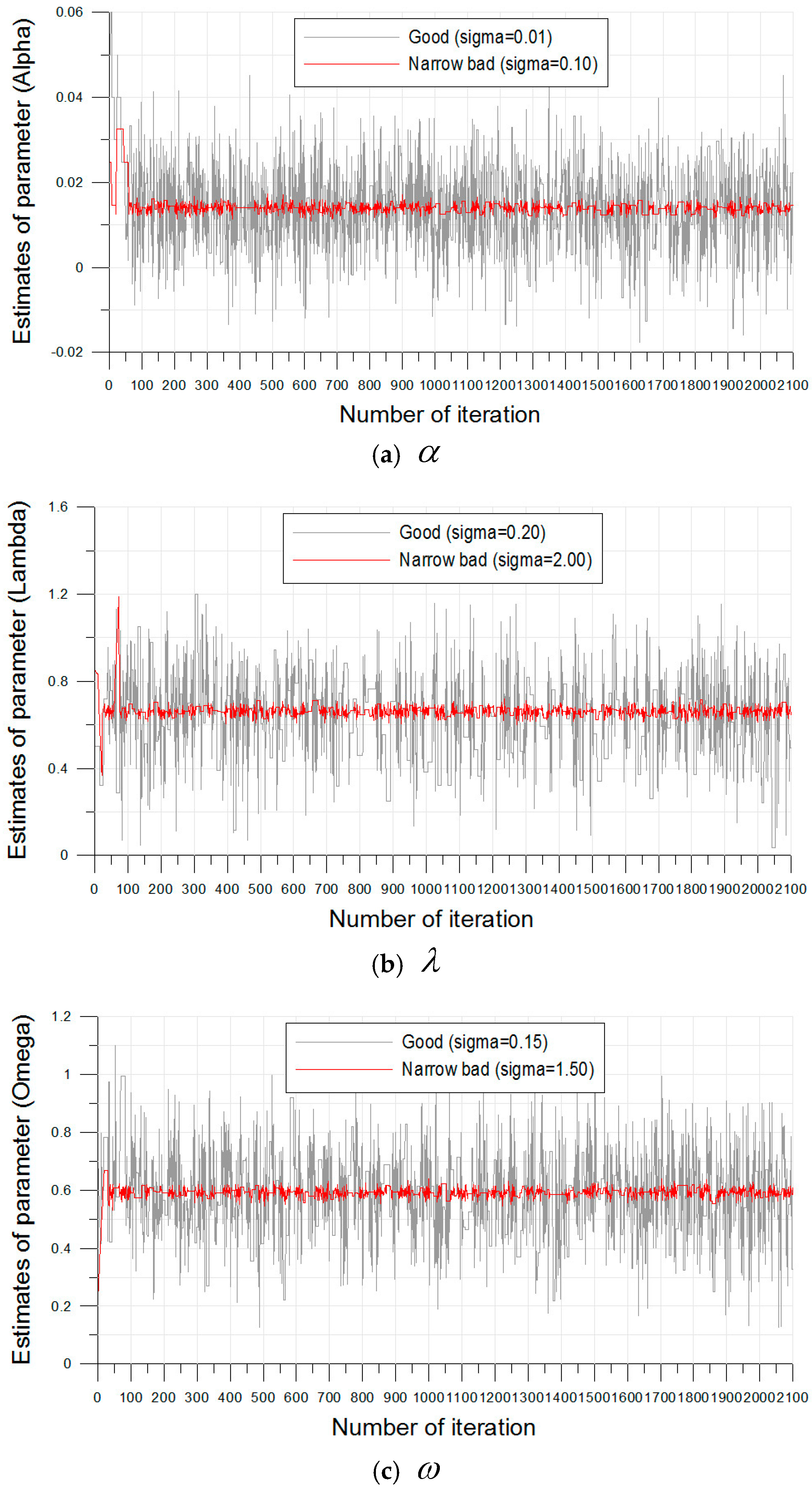
The Metropolis–Hastings algorithm coded on Matlab (Matrix laboratory, R2010a, MathWorks) generated 2100 estimates from the posterior distribution using the Bayesian ZIGP model (Equation (8)). In this posterior distribution, the likelihood function (Equation (7)) and the two prior distributions for groups 1 and 2 (Equations (13) and (14)) were used. Moreover, “burn-in”, which describes the number of estimates to be excluded in the total estimates, was 100. The mathematical background for range to perform “burn-in” is another issue. The range of excluded estimates was decided subjectively by trace plot in this study. Hence, only 2000 estimates were used to analyze the statistical characteristics of the occurrences of the torrential rainfalls in the Daegu and the Busan rain gauges. Moreover, , , in the normal type proposal distribution for the three ZIGP parameter were fixed first by two values ( = 0.01 and 0.10; = 0.20 and 2.00, = 0.15 and 1.50).
Figure 5 shows the trace plots for the results of the estimates of the three parameters in the Bayesian ZIGP model. In the estimation procedure, if
is too large, then the most proposed estimates will be rejected and the chain will not move at all. In addition, if
is too small, then the most proposed estimated will be accepted, but they will represent very small movements and finally the chain will not mix well [
38]. These two cases are called “poor mixing”.
In the case of = 0.10, = 2.00, and = 1.50, the acceptance rate was approximately 5.5%, and this result showed that the almost proposed estimates were rejected and the chain did not move (poor mixing). However, in the case of = 0.01, = 0.20, and = 0.15, the acceptance rate was 38.5%, and this value showed good mixing. The results of the three parameters for the Busan rainfall gauge were almost the same as that of the Daegu rainfall gauge. Hence, it was suggested that the selected parameters, , , by trial-and-error were reasonable for the simulation of the estimates.
In this study, three additional diagnostics (Gelman and Rubin diagnostic, Rafter and Lewis diagnostic, and Geweke diagnostic) were used to check the convergence of the generated estimates via the Metropolis–Hastings algorithm. In the Gelman and Rubin diagnostic, the convergence of the algorithm can be satisfied when the value is close to one. In the case of Rafter and Lewis, the diagnostic was greater than five, and the chain obtained using the Metropolis–Hastings algorithm can be considered poorly mixed. Moreover, in the Geweke diagnostic, if the test statistic is outside the 95% confidence interval, the algorithm can be considered to fail the convergence. The 95% confidence interval is usually used in engineering and scientific analysis.
Table 7 gives the results of the three diagnostics obtained using Gelman and Rubin, Rafter and Lewis, and Geweke. In this table, it was also suggested that the parameters
,
,
selected via trial-and-error were reasonable.
6. Result and Comparison between the Five Models
The five statistical models POI, GPD, ZIP, ZIGP, and Bayesian ZIGP were applied to the torrential rainfall data observed from the Daegu and the Busan rain gauges.
Table 8 gives the final estimated parameters of the five models. In
Table 8, the weighting parameters
for the ZIP, ZIGP, and Bayesian ZIGP models were 0.6163, 0.6144, and 0.5981 at the Daegu rain gauge and 0.5800, 0.5727 and 0.5301 at the Busan rain gauge, respectively. These results show that the estimated weighting parameter
obtained using the Bayesian ZIGP model was the smallest in two gauges. Moreover, the value obtained using the ZIP model was the largest in the two gauges.
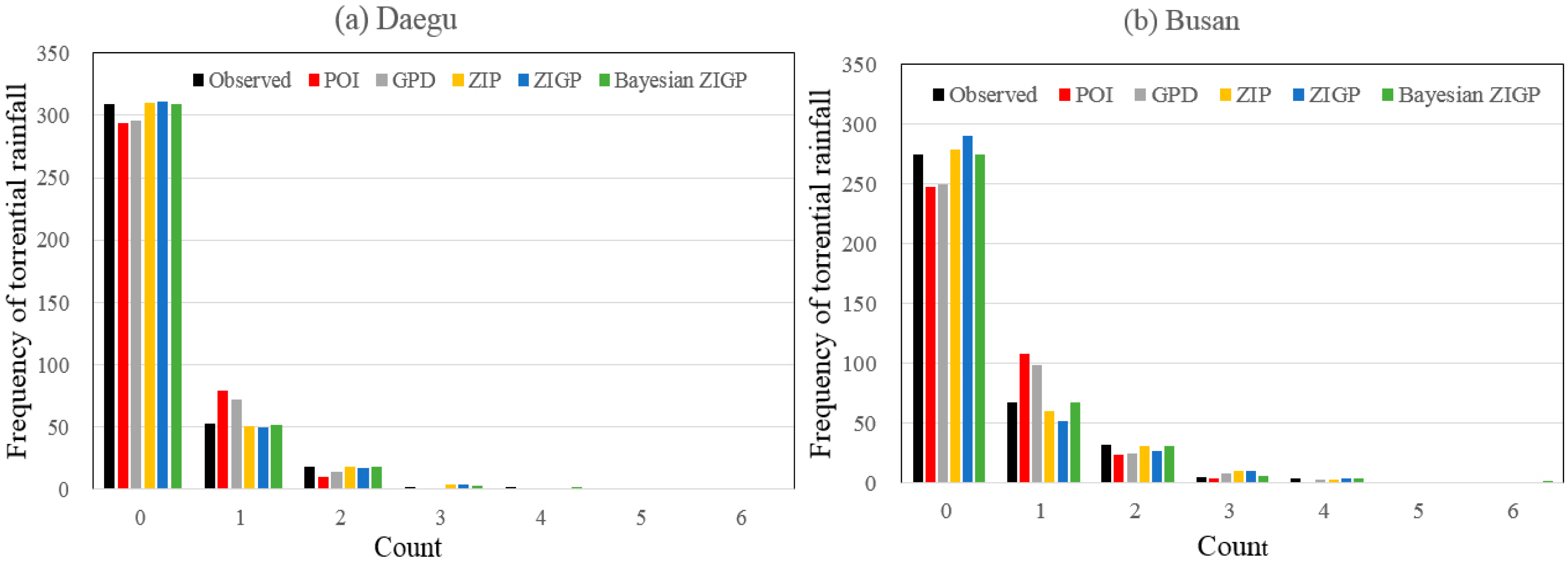
Table 9 and
Figure 6 give the observed and the fitted frequency distributions obtained from the five different models. In the Daegu rain gauge, the POI and GPD models could not provide adequate fitted results to the observed data. In particular, the two models underestimated the number of torrential rainfalls at Count 0 and overestimated at Count 1. Hence, it was concluded that the results obtained from these cases had the same conclusions as that of the earlier studies [
28]. From these results, it was known that the frequency of the number of zeros could not be fitted using the POI and GPD methods when the frequency
was significantly high. Finally, it was suggested that the application of the POI and GPD models to predict the occurrence of extreme torrential rainfall data should be avoided despite their simplicity. Although, the POI and GPD models failed to simulate the observed data, ZIP, ZIGP, and Bayesian ZIGP models could provide reasonable results for the observed data.
In the Busan rain gauge, the results obtained using the POI and GPD models were the same as those of the Daegu rain gauge. However, the results obtained using the ZIGP model were different from those in the Daegu rain gauge. In
Table 9 and
Figure 6, it was shown that the ZIGP model overestimated the number of torrential rainfalls at Count 0 and underestimated at Count 1. These conflicting results of the Daegu rain gauge were due to the estimation method used in the ZIGP model. Angers and Biswas [
24] argued that the classical statistical inference procedures, such as the MLE and large sample approximation of a confidence interval, were not always suitable to make inferences of the parameters in the ZIGP model. In addition, the advantages of Bayesian approach were reported by many manuscripts in the field of statistical hydrology [
34,
35,
38,
62,
63]. Hence, it was concluded that the ZIGP model used for the estimation of the number of torrential rainfall data might not always provide accurate results. However, the Bayesian ZIGP model fitted the observed data on all counts except Counts 1 and 3 at Daegu rain gauge and Counts 2 and 3 at Busan rain gauge. In particular, only the Bayesian ZIGP model simulated the number of torrential rainfall occurrence at Count 6 accurately. Hence, in the Daegu and the Busan rain gauges, the results of the Bayesian ZIGP model with the informative prior distribution were the best. Moreover, the results obtained using the ZIP model were similar to those obtained using the Bayesian ZIGP model. Hence, it was concluded that the Bayesian ZIGP model could be a reasonable choice to analyze the number of torrential rainfall data. In addition, the ZIP model could be recommended as an alternative choice from the viewpoint of practicality because the procedure of the Bayesian ZIGP model using an informative prior distribution was complex.
7. Conclusions
As already mentioned in the Introduction, the occurrences of torrential rainfall events due to climate change have increased drastically during the last two decades. The identification of a statistical property to evaluate the occurrences of torrential rainfalls is very important for water resource management because the natural disasters due to torrential rainfall threaten the economic stability and cost human lives. Hence, the objective of this study is to identify the statistical characteristics of the number of torrential rainfall occurrences.
In general, POI has been applied to model the occurrences of rainfall. However, one of the difficulties of applying the probability distribution, such as the Poisson model, is that the data pertaining to rainfall events are random variables with exact zeros. Hence, POI often underestimates or overestimates the observed rainfall occurrences because of the additional or fewer zeros. To overcome this problem, the concept of the ZIP and ZIGP models was developed. Moreover, the Bayesian framework using the zero-inflated concept was developed to fit the data more accurately. However, only few studies have used the zero-inflated concept for rainfall analysis despite its scientific advantages.
Hence, in this study, five different models, POI, GPD, ZIP, ZIGP, and Bayesian ZIGP, were developed and compared to determine the efficiency of the zero-inflated concept in modeling the occurrences of torrential rainfall events. Moreover, in the procedure of the Bayesian ZIGP model, the informative prior distributions were elicited to provide more accurate and realistic results. The empirical Bayes method was applied to elicit the informative prior distributions, and the cluster analysis with k-means algorithm was applied to group the homogeneous rainfall gauges.
The daily rainfall data during the 32 years (1983–2014) were collected at two rain gauges (Daegu and Busan) and additional ten daily rainfall data during the same years were collected to apply the empirical Bayes method to elicit the informative prior distributions. From the collected data, the number of months for which the torrential rainfall occurred more than once during a month was calculated at each rainfall gauge. After the calculation of the frequency distribution, the five developed models were applied to each rainfall data. In the Bayesian ZIGP model with an informative prior distribution, the estimates from the posterior distribution were sampled using the Bayesian MCMC scheme via Metropolis–Hastings algorithm.
The results showed that the POI and GPD models, which have been frequently used to fit the data pertaining to rainfall occurrences, could not provide adequate results for the observed data. Hence, it was founded that the application of the POI and GPD models for the rainfall-occurrence modeling should be avoided despite their simplicity. In addition, it was concluded that the ZIGP model along with the MLE might not always provide accurate results. Finally, it was suggested that the Bayesian ZIGP with an informative prior distribution could be used as a reasonable choice to analyze the occurrences of torrential rainfall at the two rain gauges in South Korea. In addition, the ZIP model can be recommended as an alternative because the Bayesian modeling used in this study was considerably difficult.
The focus of this study was to find the most accurate statistical model on the past torrential rainfall data in South Korea. In addition, it is necessary that the trend of future torrential rainfall due to climate change should be identified because this change can occur the severe natural disaster. Therefore, in future, the torrential rainfall occurrences in climate change scenarios such as RCPs (Representative Concentration Pathways) can be analyzed by the suggested statistical models, Bayesian ZIGP and ZIP, in this study.


