Building a High-Precision 2D Hydrodynamic Flood Model Using UAV Photogrammetry and Sensor Network Monitoring

Abstract

This paper explores the potential of the joint application of unmanned aerial vehicle (UAV)-based photogrammetry and an automated sensor network for building a hydrodynamic flood model of a montane stream. UAV-based imagery was used for three-dimensional (3D) photogrammetric reconstruction of the stream channel, achieving a resolution of 1.5 cm/pixel. Automated ultrasonic water level gauges, operating with a 10 min interval, were used as a source of hydrological data for the model calibration, and the MIKE 21 hydrodynamic model was used for building the flood model. Three different horizontal schematizations of the channel—an orthogonal grid, curvilinear grid, and flexible mesh—were used to evaluate the effect of spatial discretization on the results. The research was performed on Javori Brook, a montane stream in the Sumava (Bohemian Forest) Mountains, Czech Republic, Central Europe, featuring a fast runoff response to precipitation events and that is located in a core zone of frequent flooding. The studied catchments have been, since 2007, equipped with automated water level gauges and, since 2013, under repeated UAV monitoring. The study revealed the high potential of these data sources for applications in hydrodynamic modeling. In addition to the ultra-high levels of spatial and temporal resolution, the major contribution is in the method’s high operability, enabling the building of highly detailed flood models even in remote areas lacking conventional monitoring. The testing of the data sources and model setup indicated the limitations of the UAV reconstruction of the stream bathymetry, which was completed by the geodetic-grade global navigation satellite system (GNSS) measurements. The testing of the different model domain schematizations did not indicate the substantial differences that are typical for conventional low-resolution data, proving the high reliability of the tested modeling workflow.

1. Introduction

The rapidly evolving techniques for the precise surveying and monitoring of dynamic processes are providing new types of data for hydrological research with the potential for obtaining a better explanation of the dynamics of hydrological and fluvial processes [1]. In hydrological research, these are applied mainly to the acquisition of accurate and up-to-date spatial information on the riverscape and to the automated monitoring of hydroclimatic processes with high precision and a high sampling frequency [2].

The emerging technologies for field surveying and monitoring in the geosciences, such as unmanned aerial vehicles (UAVs; e.g., drones) and automated sensor networks, bring the opportunity to cover remote new types of data sources with high spatial accuracy. In addition to the high levels of the spatial and temporal resolutions and accuracy of the data acquisition, these technologies bring a substantial improvement to the flexibility of the data acquisition and the design of the monitoring campaigns.

The coupling of the advanced spatial and monitoring data with hydrologic and hydraulic modeling make it possible to schematize the processes in a very detailed way. The appropriate spatial and temporal discretization and model conceptualization could significantly reduce the uncertainties in the description and in modeling runoff and fluvial processes [3].

The high spatial and temporal resolutions of the data together with the high operability in their acquisition are augmenting possibilities for the application of complex hydrological models in areas that are not covered by conventional data sources. Typically, this applies to small catchments, where high detail in the spatial and temporal resolutions is necessary for the reliable simulation of processes, and to remote areas that suffer from a lack of monitoring, for example, in montane areas [4].

The major leap in the acquisition of spatial information of ultra-high spatial resolution is related to the development of the unmanned aerial systems (UASs; e.g., drones) for image acquisition and digital photogrammetric processing. UAS technologies enable the rapid and flexible acquisition of high-quality data for different applications in the geosciences, ranging from landscape ecology, vegetation studies, and geomorphology to hydrology [5,6,7]. Using UASs for operational surveying results in a significantly higher spatial accuracy and operability of acquisition compared to traditional aerial photogrammetry [7,8]. For applications in hydrology, the key benefit is the ability to build seamless ultra-high-resolution three-dimensional (3D) terrain models of complex segments of stream channels with a level of detail sufficient for even detailed analyses of the runoff and fluvial processes, which can be further combined with terrestrial Light Detection And Ranging (LiDAR) scanning [9].

The development of efficient algorithms for photogrammetric processing, such as the structure from motion (SfM) [10,11] and semi-global matching (SGM) [12] algorithms, have enabled the use of non-metric cameras for 3D reconstruction of the landscape and have facilitated in the development of photogrammetric tools. The basic photogrammetric operations, including the generation of orthoimages and digital surface models, have become available as desktop software suites as well as cloud-based computing services [13,14].

For research in fluvial geomorphology, UASs represent a flexible tool for the rapid mapping and acquisition of high-resolution data for the 3D reconstruction of floodplains and river channels [6,9]. Despite their benefits, several limitations persist. Two of these are of particular importance for applications in undisturbed natural environments: (i) the effect of vegetation cover, and (ii) the reconstruction of submerged zones. Progress in point cloud classification techniques enables separating the vegetation from the terrain reliably [15], but there are still substantial limitations to the efficient 3D reconstruction of areas with dense vegetation. For the mapping of riverscapes, this is an important issue, particularly in forested areas, where the river banks are often completely covered by vegetation. The second limitation is the inability to properly reconstruct the submerged zone of channels.

Although there have been techniques developed enabling the 3D reconstruction of the river bottom from UAV imagery [8], these are limited to specific conditions, in particular, non-turbulent flow, low turbidity and shallow channels [16]. Hence, even in small streams, the building of complex 3D models of channels still often requires auxiliary data for the submerged zone, typically based on geodetic profiling. For hydrodynamic models, the detailed topographical reconstruction of the stream bathymetry predetermines the accuracy of the hydrodynamic modeling [17]. Inaccurate description may result in imprecise calculations of the hydrodynamic properties and further propagation of the errors in calculations of the morphological changes or consequent transport of sediment.

In hydrological research, technologies for the automated monitoring of the dynamics of runoff by automated sensor networks have an increasingly important role in experimental research [1]. The automated monitoring of surface and groundwater runoff processes enables the acquisition of data with high frequency and accuracy [4,18]. A high frequency of sampling with a high level of accuracy provides a new qualitative level of hydrological data, enabling a detailed analysis of the dynamics of runoff processes [19,20]. This type of monitoring introduces the possibility to investigate highly dynamic processes with an unprecedented level of detail. The coupling of monitoring devices with communication modules using mobile communication network (GSM) or satellite telemetry enables online access to the observed data in the near-real-time regime, even in remote areas with limitations of access.

The combined use of high-resolution 3D models with the high-frequency monitoring of hydrological processes enables the building and calibration of highly accurate hydrodynamic models for the simulation of dynamic processes in headwater or remote areas, where conventional monitoring is lacking or has an unsatisfactory quality of coverage. Despite the small scales of such experimental areas, the high density of the data results in a need for high-performance tools that are able to simulate dynamic processes with a high spatial resolution and a small time-step. Such an application is enabled by the recent progress in model development as well as by the progress of computational performance, including graphic processing unit (GPU) acceleration or grid-based computing [21]. The theoretical concepts and practical tools for numerical modeling have been developed and used in operative and prognostic hydrology since the 1960s. For physically based models, the numerical modeling is based on the solution of partial differential equations or ordinary differential equations for empirical models [22] in various dimensions. A differential relationship expressing physical laws requires a solution with a given level of discretization of the space–time continuum. With the increasing availability of high-computational-performance workstations, benefiting from multi-core CPUs and GPU acceleration, the applications tend to create complex descriptions of the natural environment using a fine computational network or mesh.

The complex model inputs and calibration place high demands on the quality and resolution of the field data [23]. The modeling of the fluvial dynamics problem suffers from both the data needed and its availability. Recent developments in sensor technologies and close-range remote sensing may help to bridge this gap by delivering accurate and reliable data for the building and calibration of the simulation models.

The aim of this research was to explore the potential of coupling the advanced methods for the acquisition of accurate spatial data by UAS photogrammetry and the high-frequency monitoring of runoff processes to build a highly precise hydrodynamic model able to reliably simulate the dynamics of runoff processes. Particular focus was given to the identification of the limiting aspects of the individual techniques and of the workflow to discuss the broader applicability of this approach in experimental research and water management.

The particular goals of this study were (1) to define a workflow for coupling UAV photogrammetry with automated sensor networks for building high-precision hydrodynamic models; (2) to verify the applicability of the approach to an observed major flood event; and (3) to test the sensitivity of the model, on the basis of ultra-high-spatial resolution data, to different types of horizontal-plan schematizations.

2. Materials and Methods

2.1. Study Area

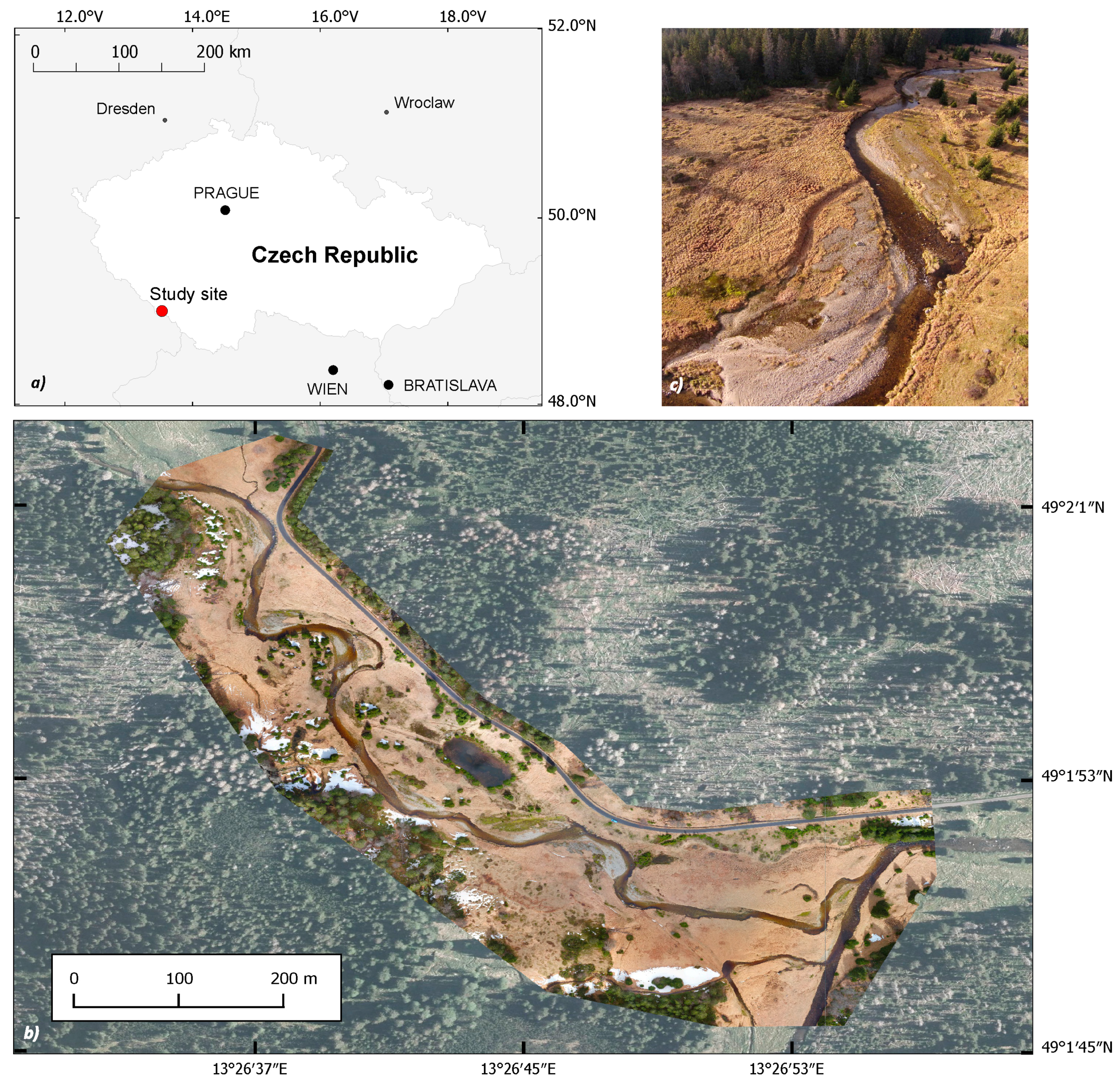
The case study is located at Javoří Brook (Šumava Mountains, Czech Republic), a small montane stream with the catchment draining an area of 11 km² at an altitude of 1172 ± 139 m a.s.l. (Figure 1). The location in the headwaters and strict conservation due to its location in the core zone of the Šumava National Park stimulate the dynamic evolution of the channel. The study is focused on a 430 m long stretch of the river channel and riparian zone, including active bank erosion structures and point bars, covered by gravel of various grain sizes [24].

The hydrological regime of the hydrological system is dominated by significant spring snowmelt, occurring from April to May [25], with frequent occurrences of low-magnitude floods resulting mostly from summer storms, regional rains and rain-on-snow events in the fall or spring period [26]. As a headwater catchment, it is the source area of large floods in the Vltava and Elbe river basin, including, for example, the extreme flood in August 2002. However, as a result of its position at the basin divide and a relatively flat topography, the flood magnitudes here are usually lower compared to those of the lowland segments of streams.

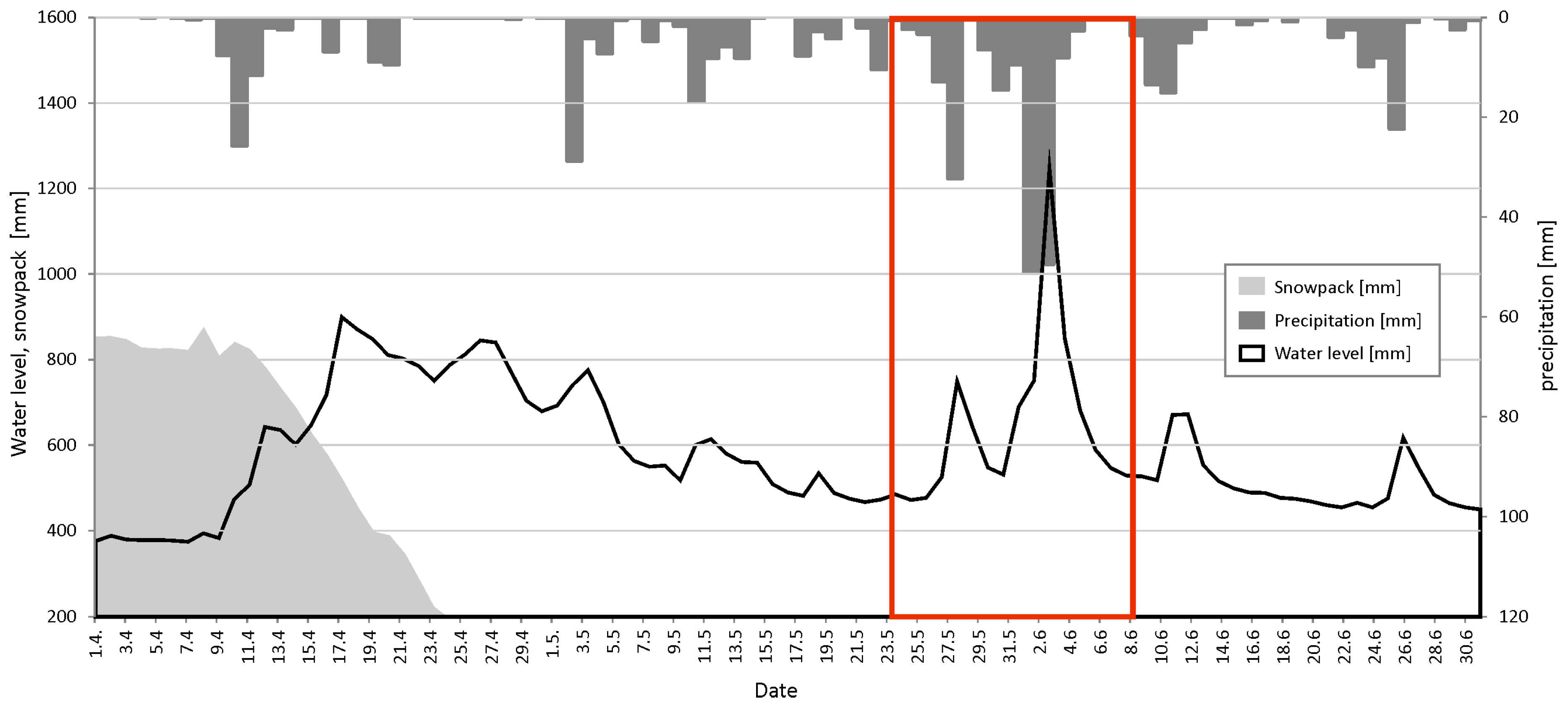
The latest significant flood hit the area in spring 2013 and was selected as a reference event for this study. The flood resulted from heavy rains reaching the basin, which was saturated by the preceding fast spring snowmelt (Figure 2). The peak flow of the Vydra at Modrava station reached on 2 June 2013 a discharge of 54.6 m³·s⁻¹ [26], corresponding to a 5–10 year flood, while in consecutive lowland segments of the Otava River, it reached the magnitude of a 20–50 year flood [27].

2.2. Applied Data Sources

Building a detailed hydrodynamic model in an experimental montane area requires the building of the key data sources from own survey and monitoring campaigns, combining different instrumental techniques, that is, UAV imaging, GNSS positioning, and automated sensor network monitoring.

The UAV imagery has been applied as a basic source of spatial information for the 3D reconstruction of the floodplain and the river channel. By means of photogrammetric processing (see Section 2.3), two basic data products were derived from it, the digital elevation model (DEM) and the orthoimage. The accurate georeferencing of the imagery was performed by the GNSS positioning of the ground control points (GCPs), used for the referencing of the imagery during the photogrammetric processing.

The 3D channel model was built by merging the DEM of the terrain above the water level, acquired by UAVs with the elevation model of the submerged zone and built using bathymetric measurements using GNSS positioning (Section 2.4). For use in the hydrodynamic model, three different geometry schematizations of the 3D channel were built and tested—an orthogonal grid, a curvilinear grid and a flexible mesh (Section 2.5)—as, despite the same data origin, these have a different effect on hydrodynamic modeling.

The automatic sensor network providing water level measurements with a sampling interval of 10 min was used as a source of information on hydrological processes and was applied as the boundary conditions of the model (Section 2.6). The water level data was converted to discharges on the basis of rating curves, built by repeated direct measurements at monitoring stations [28].

2.3. UAS Imaging and Photogrammetric Reconstruction of Floodplain

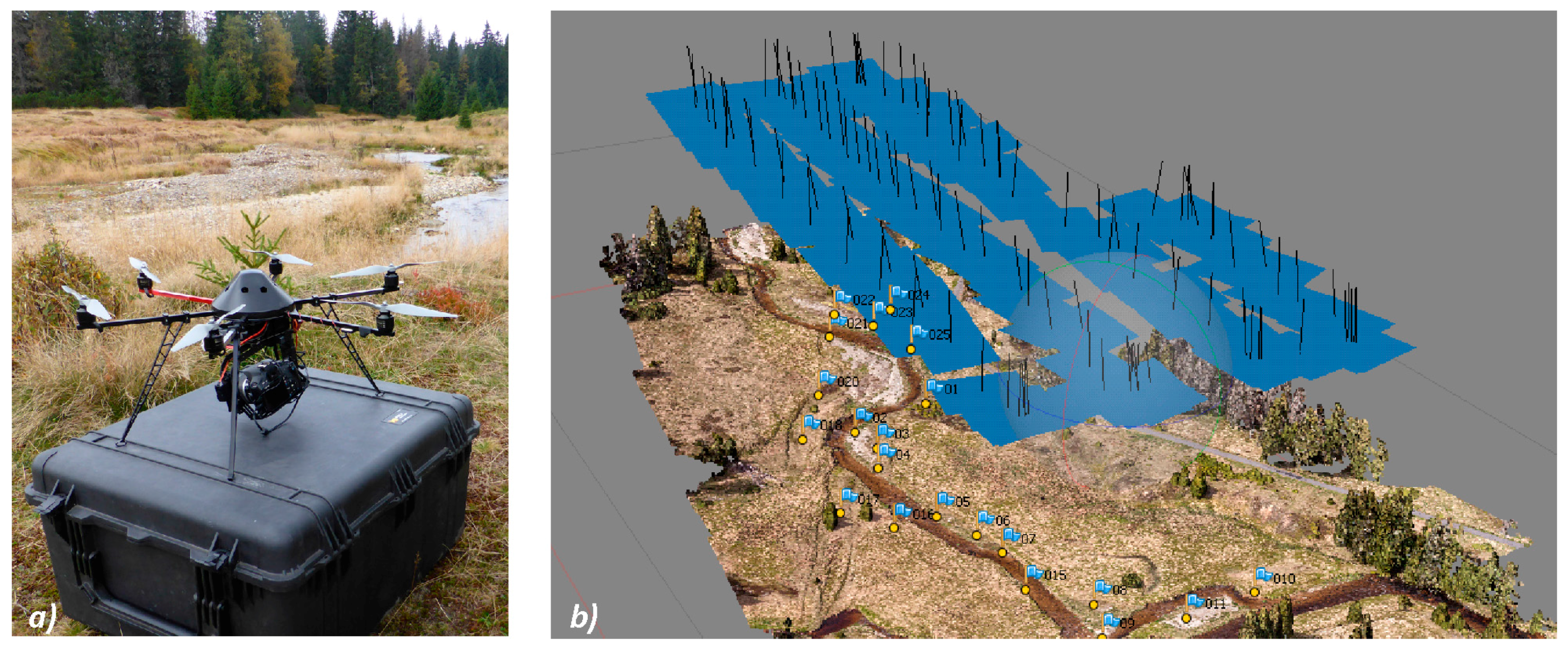
The unmanned aerial platform MikroKopter Hexa XL was used for the imaging of the study area (Figure 3a). The imagery was acquired by the non-metric Canon EOS 550D camera with a calibrated Voigtländer 20 mm prime lens. The imaging campaign was realized in May 2013, one month before the flood, and is analyzed further in the study. The flight was performed at an altitude of 88 m in the form of a grid (Figure 3b) and resulted in the acquisition of 96 images with a 70% front and side lap.

GNSS positioning was used to capture the locations of 12 GCPs distributed unevenly over the study area (Figure 3b). The positioning of the GCPs was done using a Topcon HiperSR device with Real Time Kinematic (RTK) corrections, achieving a horizontal accuracy of 1.8 cm and a vertical accuracy of 2.5 cm (

Table 1. Parameters of the imagery and photogrammetric processing.

Parameter	Value
Number of images	41
Flying altitude (m)	88
Ground sampling distance (cm)	1.5
Number of ground control points	12
Number of tie points	215,803
Error of the image coordinates (pix)	0.67
Point density (points/m2)	201
The average error in Z (m)	0.001
Root-mean-square error (RMSE)Z (m)	0.021

).

The photogrammetric processing was done using Agisoft Photoscan Pro software, employing the structure from motion (SfM) algorithm [10] for the reconstruction of the 3D space from the overlapping images. The SfM method stems from the basic principle of stereoscopic photogrammetry, resolving a 3D structure from the set of overlapping images. The SfM method uses images acquired from multiple viewpoints to restitute the 3D geometry of an object or surface and diverges significantly from traditional photogrammetry. Unlike the conventional approaches relying on strips of overlapping images acquired in parallel flight lines, SfM allows for reconstructing the 3D space from unstructured imagery [11]. The multi-view matching method performs very well for oblique images as well as for classic aerial images with forward and side overlap. On the basis of known exterior orientation parameters, the terrain reconstruction is performed. The semi-global matching (SGM) method [12] was used, as it produces very precise dense point clouds of the surface. This recently emerging method has a strong theoretical background from the field of computer vision. The per-pixel autocorrelation matching is the basis for point cloud generation. This approach combines the concepts of global and local stereo methods for accurate, pixel-wise matching [13]. As the SfM and SGM methods perform efficiently for nadir aerial imagery as well as for oblique images, these have become a standard solution available in recent photogrammetric software suites such as, for example, Agisoft Photoscan, Pix4D, and MicMac [14,15,16].

Using the standard processing chain of the Agisoft Photoscan software, alignment of the unstructured imagery, georeferencing using GCPs and the building of a dense point cloud were performed. On the basis of the dense point cloud, the DEM and orthoimage were built.

2.4. 3D Reconstruction of the Stream Channel

The bathymetric reconstruction of the stream channel and the riparian zone was performed on the basis of three data sources: (i) conventional DEM, based on aerial LiDAR scanning; (ii) UAV-based DEM; and (iii) the bathymetric measurements. As none of these datasets themselves can reflect the complexity of the stream channel morphology at the required level of detail, the 3D reconstruction of the stream channel was based on their fusion.

The conventional DEM, based on aerial LiDAR imaging [29], is available as a reference dataset, covering the whole area of the basin, including the floodplain. The DEM, representing the most detailed complex terrain model covering the Czech Republic, results from aerial LiDAR mapping acquired in 2009–2013 and is supplied in two products with different resolutions. The DMR4G model, with 5 × 5 m resolution, was launched in 2014, and the DMR5G, with 2 × 2 m resolution, was launched in 2016. The mean vertical error for the DMR4G is 0.3 m for open areas and 1 m in forested areas, and for the DMR5G, it is 0.18 m in open areas and 0.3 m in forested areas [29]. All of the available official geospatial data products are based on the Czech national coordinate system S-JTSK (EPSG 5514, Krovak East North), representing a national standard for geodetic surveying, mapping and geospatial data products; hence this coordinate system was used as a base for this study.

The UAV-based terrain model, built using the photogrammetric reconstruction from the imagery, taken in visible spectrum in red, green and blue (RGB) spectral bands, also covers the flooded zone of the channel. The derived DEM features the variability of the elevations for the riparian zone and stream channel, and also for the submerged zone (Figure 4). However, because of the water turbidity and the highly turbulent flow in a step-pool system, the 3D reconstruction of the submerged zone of the channel cannot be considered as reliable [9].

To obtain the missing information on the bathymetry, 250 points were collected using RTK-GNSS positioning, and the resulting data points were used to build the model of the submerged zone of the stream channel. The channel model was thus built as a fusion of the available elevation data sources, designed to use the most accurate and detailed data sources available for the given riverscape segments. As the fusion of different elevation models brings step changes in data density at the transition zones, a detection of the potential outlier points was performed to eliminate them prior to further processing in order not to affect the resulting channel model. The 3D reconstruction of the stream channel and the riparian zone was, in our study, performed on the basis of the following prioritization of the UAV-based DEM, GNSS positioning, and aerial LiDAR scanning data, as follows:

(1)

The basic elevation model for the riparian zone and the stream channel, covering the zone above the water level, was the DEM, derived from UAS photogrammetry with vertical and horizontal resolutions of 1.5 cm. The UAS model has covered the active zone of the fluvial processes simulated by the model.

(2)

The data for the submerged part of the channel was completed by measurements using the GNSS positioning device, achieving comparable accuracy to the UAS DEM. The points were collected with respect to the dominant break lines in the bed topography. The density of the collected points varied in accordance with the terrain inflection points. The samples were primarily located along cross-sections placed along the channel in a step of 3–10 m. The obtained cloud of Z points was processed in a Triangulated irregular network (TIN) including hard lines defined according to the channel properties (step-pool geometry) derived from the UAV imagery. Rather than the cross-sections, all dominant structures of the channel were sampled.

(3)

The surrounding parts of the floodplain were filled with the conventional DEM available for the area, the DMR4G (ČÚZK).

2.5. Horizontal-Plan Schematization

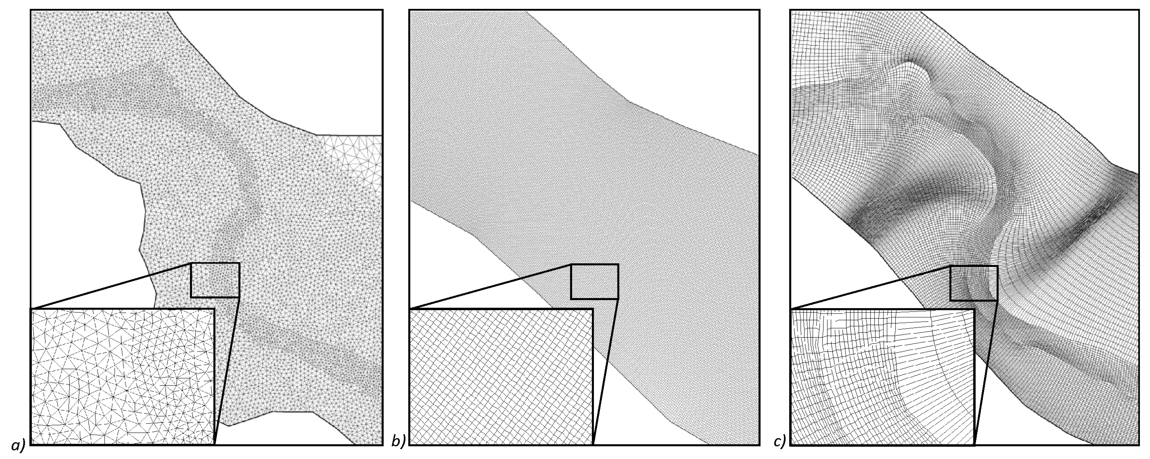
As the digital channel model is based on data from different sources with varying point densities, an appropriate horizontal-plan schematization is of significant importance for hydrodynamic modeling. In our study, three types of horizontal-plan schematizations were tested: (i) a flexible mesh, (ii) an orthogonal grid, and (iii) a curvilinear grid (Figure 5). Each type of horizontal-plan schematization has specific features that are beneficial under given conditions and for specific needs.

(i)

A flexible mesh is constructed of triangular or quadrangular elements of variable size (Figure 5a). Such a discretization of the model domain represents precisely the shape of the terrain and reduces the total number of computational points by increasing the element area at the zones without terrain variations or that are of less interest for the problem under focus [17]. Each element contains all domain parameters averaged over the area and enters the computational scheme as a point in the center. The results are calculated and stored for the central point.

(ii)

Discretization using an orthogonal grid is the basic and most common representation of the terrain. The domain is based on equidistant steps of square or rectangular cells that contain averaged parameters of the terrain entering the shallow water equations (Figure 5b). To describe the highly varying terrain well, the grid has to be very dense, even in the areas of less interest. The reduction of the cell count affecting the performance of the simulation is enabled by prolonging the rectangles in the direction of the main flow. Nevertheless, in a meandering reach, prolongation is not appropriate, because of the periodic variation of the flow direction.

(iii)

A curvilinear grid is applied in cases requiring a reliable representation of naturally curved channel properties. It is represented by an orthogonal grid coupled with the geometry grid of the varying shape of the network (Figure 5c). Each cell has, in reality, a trapezoidal shape but nevertheless enters the model in the numerical scheme with a rectangular representation [17]. Such an approach was constructed to keep the general shape of the meandering rivers.

2.6. Hydrological Input Data

The input dataset for the hydrodynamic model setup, calibration, and reconstruction of the 2013 flood event was provided by an automated water-level monitoring network, which has operated in the basin since 2006 by Charles University [4]. For the Javoří Brook, data from three monitoring stations were used. The upper boundary is represented by the confluence of the Javoří and Tmavý Brooks, located 1.2 km upstream to the simulated segment with the active meandering system, and the station at the lower bound is located 3.2 km downstream from the analyzed segment. All gauging stations are equipped with a Fiedler M4016 automatic station with US 1200 ultrasonic gauges and sample the water levels at 10 min intervals with a millimeter accuracy and with the GSM transmission of the data to cloud-based storage with online access [30]. The 10 min interval was selected as an optimum value, balancing the requirements of sufficient temporal resolution for covering the dynamic events with the volume of the observed and stored data as well as the energy consumption of the monitoring station. Capturing the water levels at 10 min intervals enables sufficient cover even for the course of short summer storms typically lasting from hours to days; at the same time, such frequency allows for uninterrupted autonomous monitoring over the winter season when the devices in remote montane areas are mostly inaccessible. The rating curves for the stations were derived by repeated direct measurements of the discharge using the SonTek FlowTracker velocimeter over 3 years.

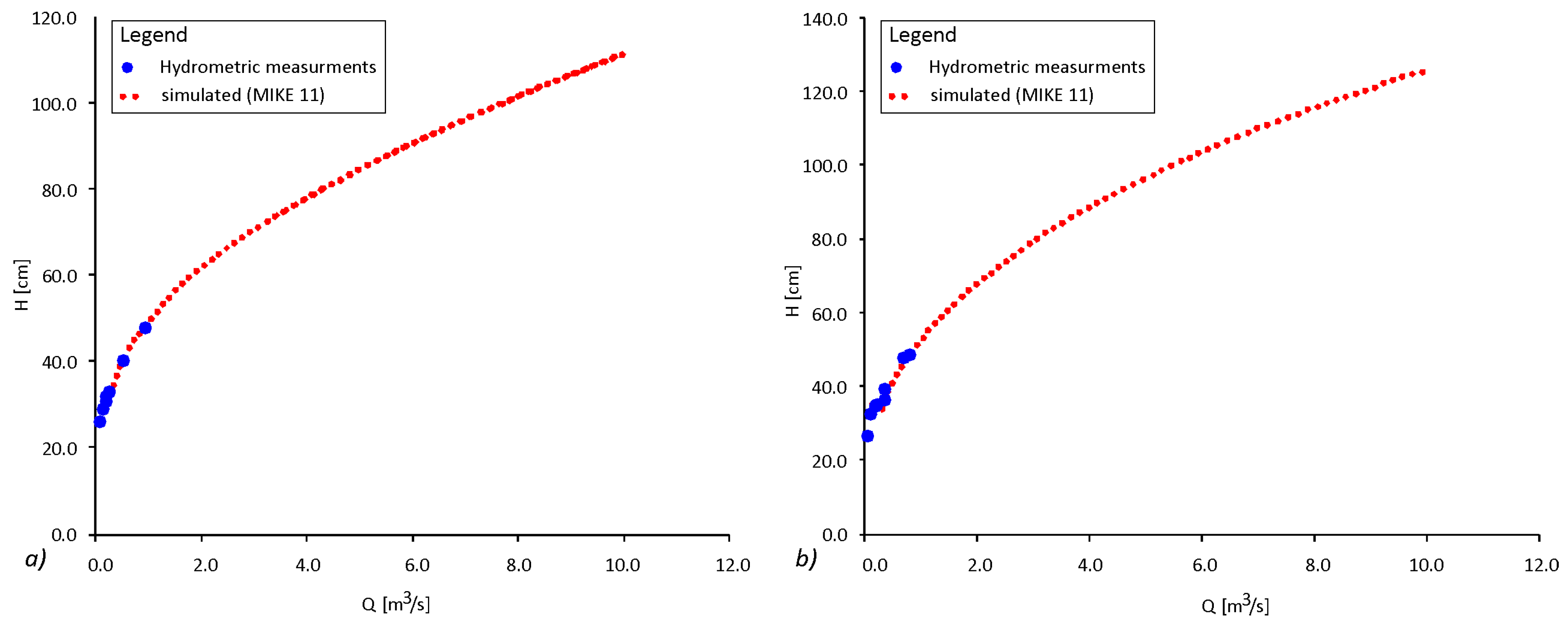
As the upper station is at the confluence of two streams (Javoři and Tmavý Brooks) without any further significant affluent, the upstream hydrograph was constructed as a compound of these two stations. The rating curve was further completed by numerical modeling to obtain the data, reaching beyond the observations and enabling the coverage of the extreme values (Figure 7). The channel properties were obtained by a field geodetic survey, and the channel roughness was optimized according to the measured data as Manning’s n = 0.05. The standard methods of extrapolation by logarithmic, exponential and power curve equations using the R² objective criteria were tested with the large deviations and magnitudes in the higher water-level area. The best fit with the measured data and the most realistic extrapolation were processed by a fully dynamic numerical simulation of the one-dimensional (1D) hydrodynamic model of the confluence with structures implemented (Figure 6).

2.7. Hydrodynamic-Model Setup and Calibration

The modeled process of a storm-driven flood wave propagation through a river reach with the rapid response of a small montane stream includes high gradients in the model domain and time variations of the boundary conditions. Therefore, the simulations were based on the fully dynamic unsteady solution of the depth-averaged shallow-water equations, requiring small time steps and a high-order solution technique for time integration and space discretization. The limitation of shallow-water equations is that the longitudinal scale of the modeled phenomenon has to be significantly larger than its vertical scale [31]. In this study, this condition was fulfilled, as the model domain covered a 430 m long stretch of the shallow stream, with its depth ranging from 0.3 to 2.4 m, meandering in a flat floodplain, where the flood waves in the June 2013 flood event lasted for more than two days (Figure 2).

As a modeling tool, the 2D flow model MIKE 21 HD was chosen as a comprehensive modeling system, enabling fully 2D flow modeling in various environments ranging from stream channels, overland flooding, and reservoirs to estuarine waters [31]. MIKE 21 is used in a broad range of applications, solving the river flood propagation at different spatial scales and variable environmental conditions [32,33,34]. MIKE 2D hydrodynamic models can use different types of the domain schematization, including a flexible mesh (MIKE 21 FM), orthogonal grid (MIKE 21), and curvilinear grid (MIKE 21 C), by applying different numerical methods for the solution; these were used for the model domain construction to evaluate the possible effect of the domain schematization on the results (

Table 2. Different characteristics of the model domain setup.

2D Model	Domain Schematization	Numerical Method	Time-Step (s) Min/Avg/Max	No. of Elements Cell Size (s) Min/Avg/Max (m2)
MIKE 21 FM HD	Flexible triangulation	Finite volume method	0.01/0.03/1	32,687
				0.1/0.5/1
MIKE 21	Orthogonal grid	Finite differences method	0.2	86,271
				0.5/0.5/0.5
MIKE 21 C	Curvilinear grid with high level of curvature	Finite differences method	0.05	31,280
				0.1/0.5/2.5

).

A cell size of 0.5 × 0.5 m was used for all approaches. The channel roughness was distinguished by three classes and was optimized during the model calibration: (1) river channel bed: 0.038; (2) unvegetated accumulations not flooded during steady-state (Qa) conditions: 0.036; (3) floodplain vegetated by grass: 0.043. The boundary conditions were based on the data obtained by the sensor network and were transferred to the time series of discharge for the upstream boundary and water levels for the downstream boundary. The hydrologic boundary conditions of the model included both dynamic (flood-wave) and Qa simulations.

The MIKE 21 and MIKE 21 C numerical scheme is based on the finite difference method for solving depth-averaged shallow-water equations in two dimensions. The time-step is set as constant for the whole simulation and the selection is based on the gradients of the terrain and flow variables. The MIKE 21 FM numerical scheme is based on the finite volume method. The time step is varied automatically according to the gradients of the terrain and flow variables. To reduce the numerical instabilities during the dynamic process, such as the fast runoff response, the time-steps have to be reduced significantly and the computation time increased dramatically, for example, in comparison with the orthogonal grid. The model calibration was carried out in a two-step process. First, the calibration of the channel bathymetry roughness was performed under Qa conditions. It was based on the comparison of depth-averaged velocities simulated with field measurements conducted by the Sontek Flow Tracker acoustic Doppler velocimeter (SonTek/YSI, San Diego, CA, USA). Second, the calibration of the flooded extent was carried out, on the basis of a comparison between the model reconstruction of the highest recorded flood event in June 2013 and field observations.

Figure 7 shows a reconstruction of a flood wave hydrograph produced by the model used for the Javoří and Tmavý Brook rating curve extrapolation. The reconstruction proves the reliability of the rating curve for predicting the whole spectrum of discharges. The difference between the discharges derived from the rating curve and the values simulated by the model of the gauges was marginal and did not exceed 6 cm. The difference is given by the generalization of the rating curve, particularly regarding the mutual influence of the streams at the confluence that could not be fully considered.

Furthermore, a sensitivity analysis was conducted using the varying roughness coefficient n within the range given in [35] for gravel bed mountain streams, using the value range of 0.05–0.03 for a non-vegetated channel, 0.047–0.029 for the accumulation bodies covered by finer material than that in the channel, and 0.071–0.030 for the floodplain vegetated by high-density grass. The interval of maximum relative possible error was observed to range from 23 ± 8% in the case of the resulting depth-averaged velocity to 30%, considering the remobilization causal discharge assessment (Figure 8). Similarly, as observed, for example, in [36], the relative error was lesser for the higher flow conditions than for the low flows at the beginning of the simulation.

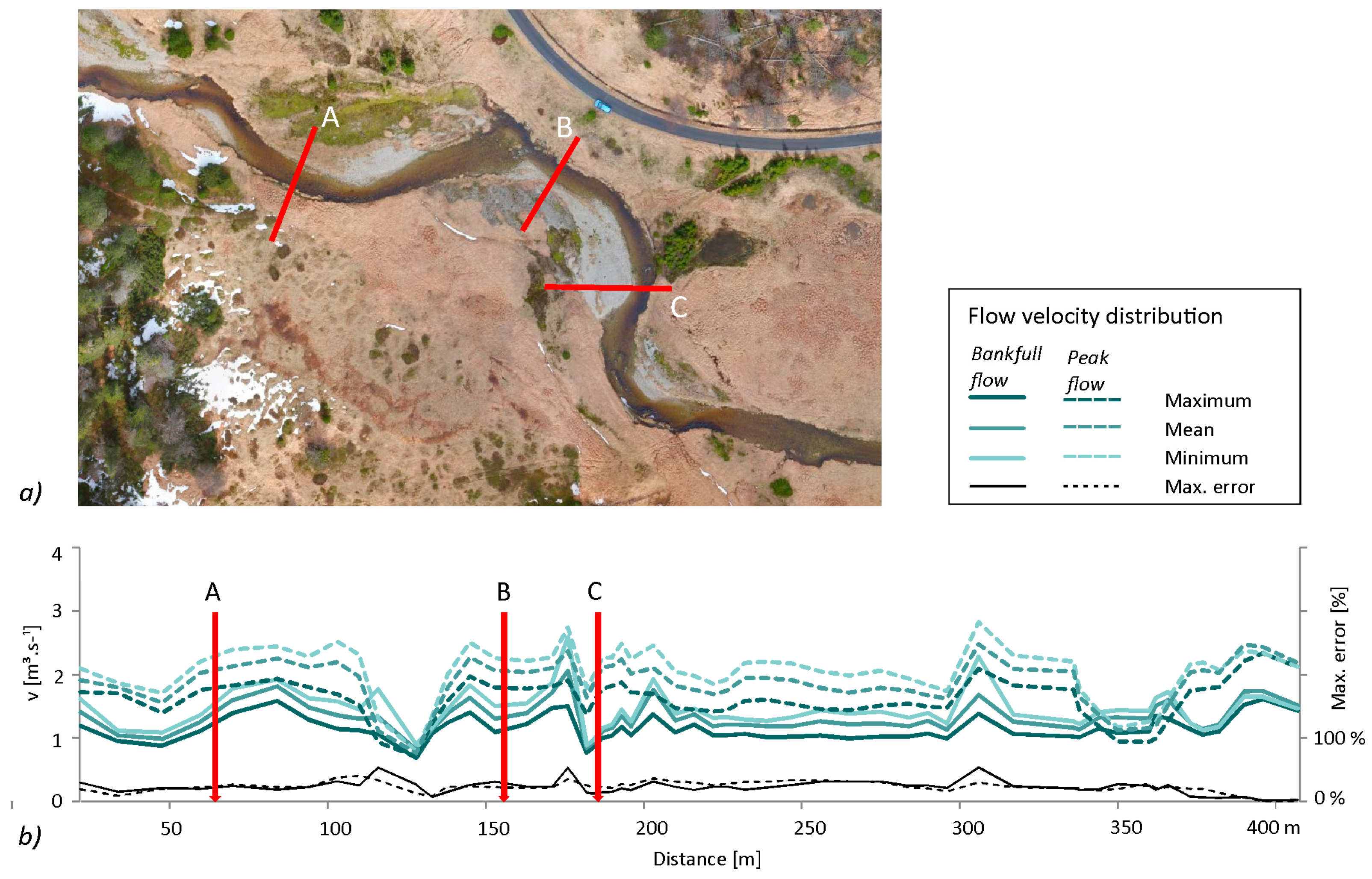
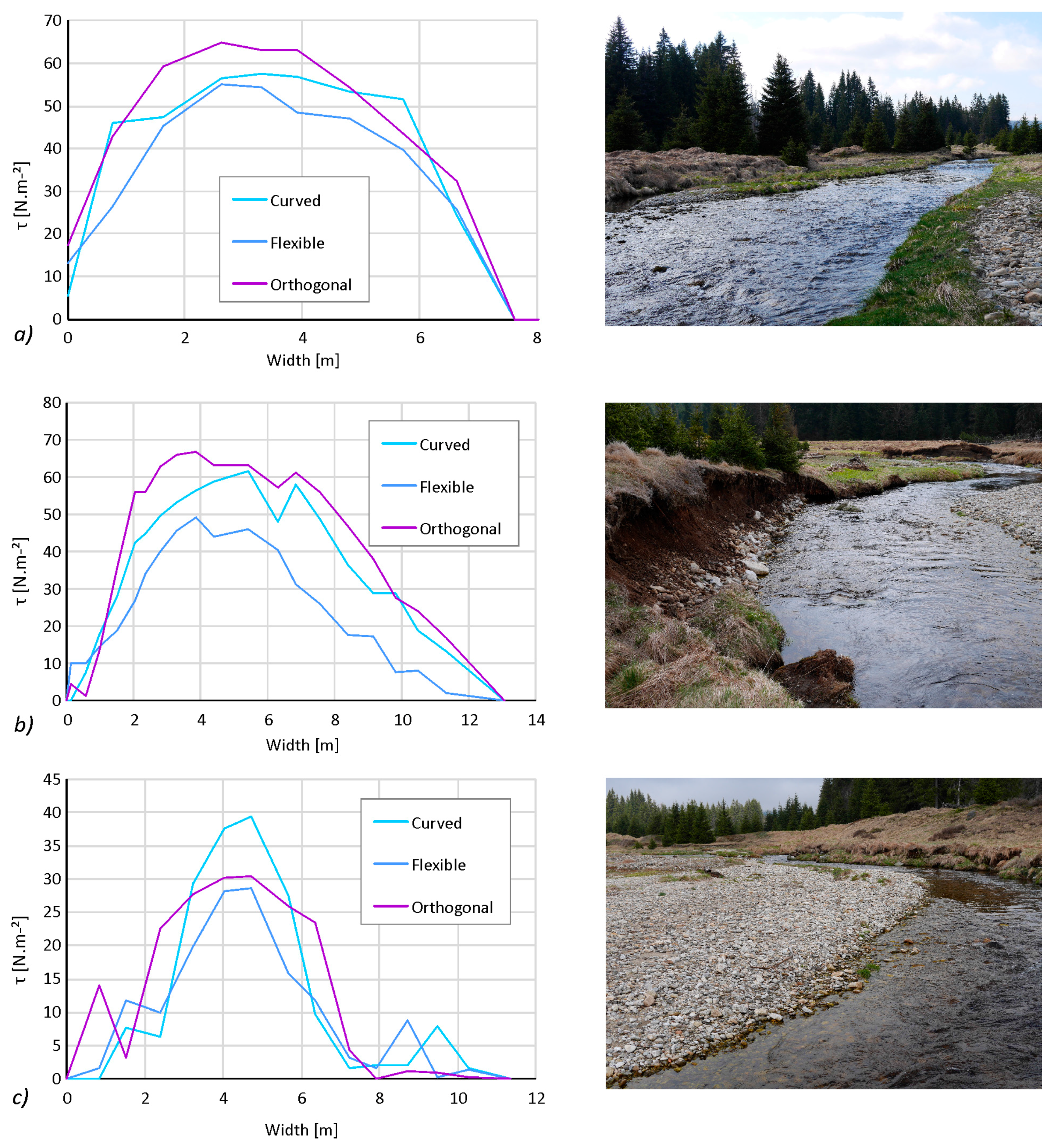
For a further comparison of the results obtained by the various types of domain schematizations, three characteristic cross-sections were selected. Cross-section A was located within the straight reach upstream of where the most significant fluvial morphology forms. Cross-section B describes the site at which the largest active left-bank failure is located. Cross-section C cuts through the subsequent reach where active sandy gravel accumulation is observed (Figure 8).

3. Results

3.1. 3D Reconstruction of the Stream Channel

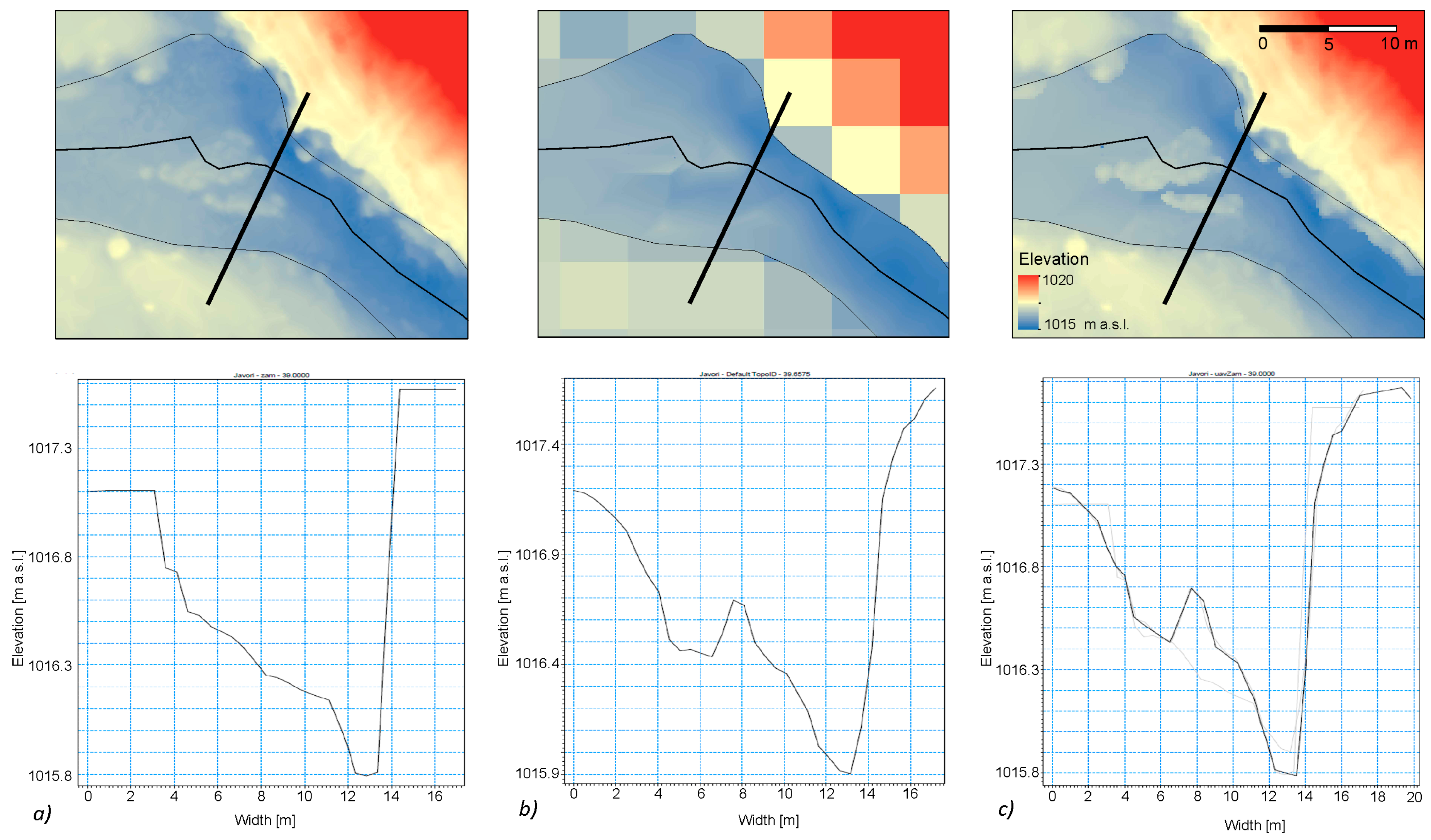
The model domain, on the basis of three different geometry definitions, was built for the analyzed stream stretch. The topographic information is represented by one characteristic value for each cell of the mesh; however, for each schematization, the topographic information was calculated differently. In the case of the flexible mesh, the cell characteristic elevation was obtained by calculating the center of gravity of each cell using the edge nodes of the specified elevation. In the case of the orthogonal and curvilinear grids, the cell elevation was specified according to the central points of the cells.

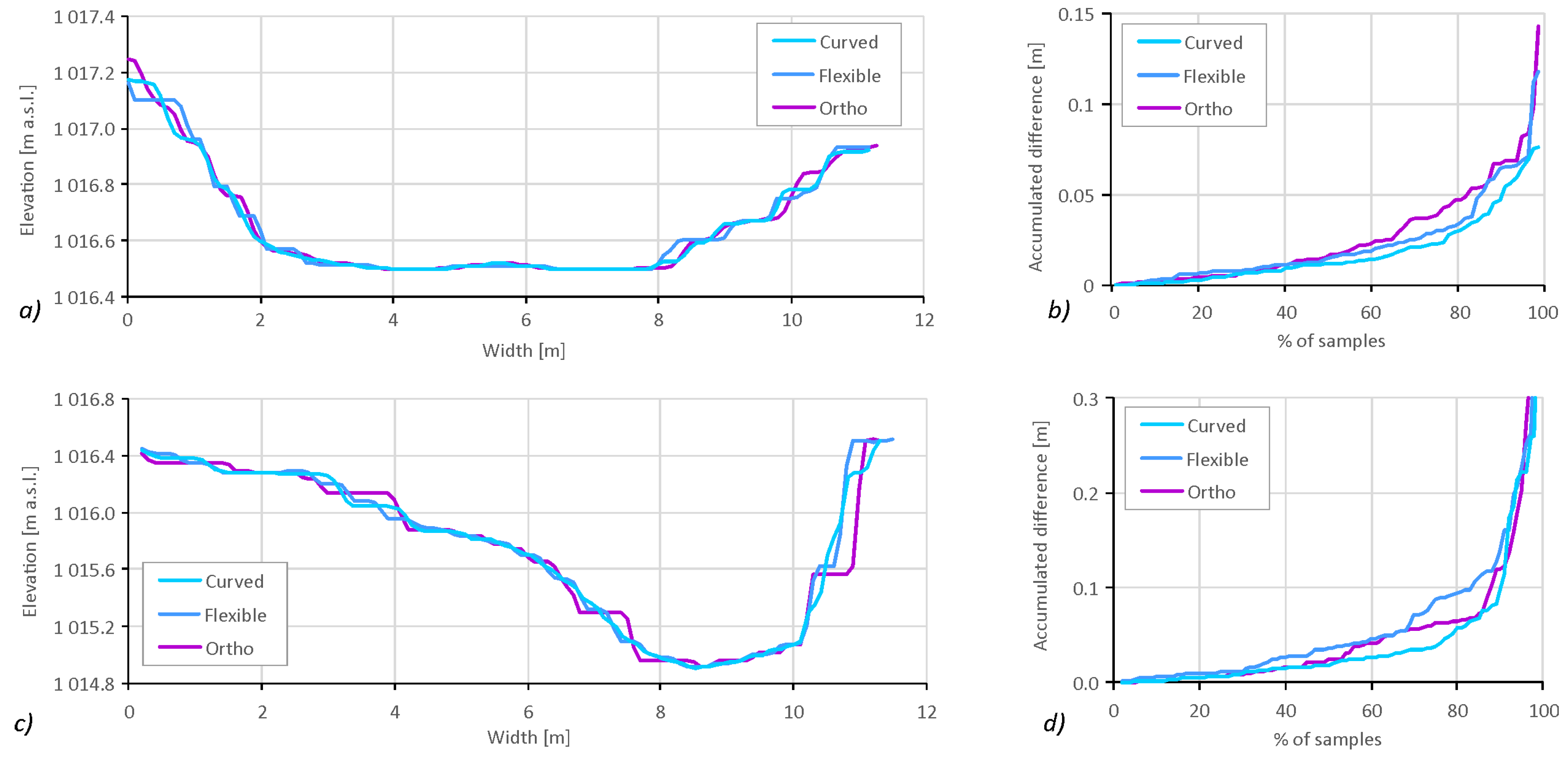
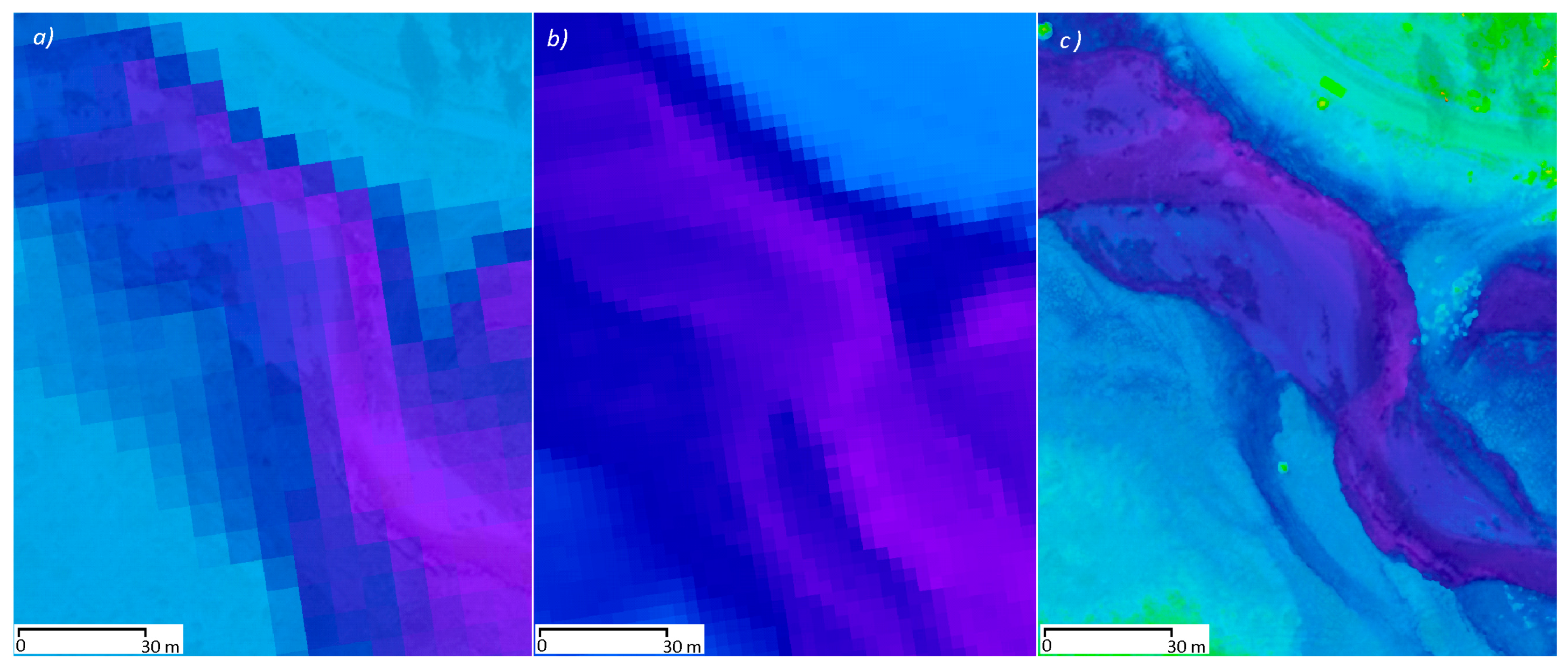
The comparison of the three types of schematizations proves the differences in the resulting channel model and, in particular, the selective effect on the different parts of the stream channel (Figure 9). The most notable differences in the channel 3D model affected the steeper parts of the stream banks, while the stream bottom, as well as the values in the upper parts of the channel, remained almost unaffected by the different schematizations. The effect of the different schematizations is illustrated by two cross-sections, representing the profiles with the lowest and largest differences, identified along the analyzed segment. In the cross-profile featuring the lowest discrepancies (Figure 9a,b), the average difference was 1.5 cm, and at only 3% of the banks were there detected differences greater than 10 cm. However, in the cross-profile with the largest differences in the analyzed segment (Figure 9c,d), the average difference reached 5 cm, while in 12% of the banks, the absolute differences in altitude exceeded 10 cm.

3.2. Hydrodynamic Reconstruction of the Flood in June 2013

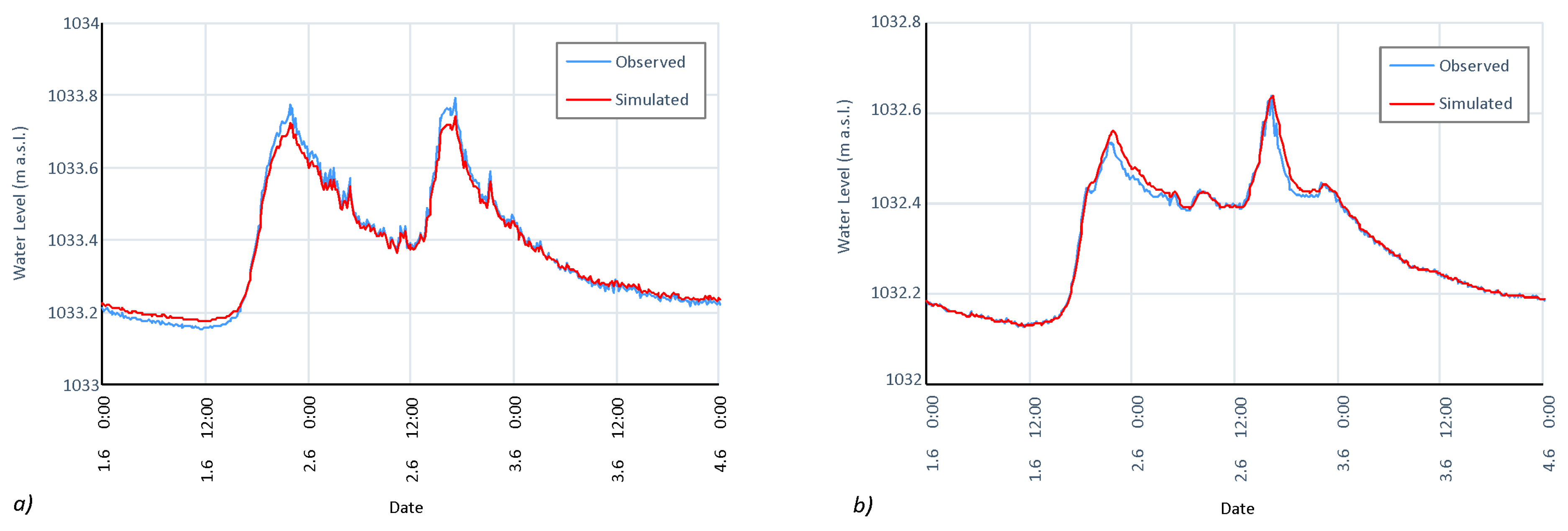
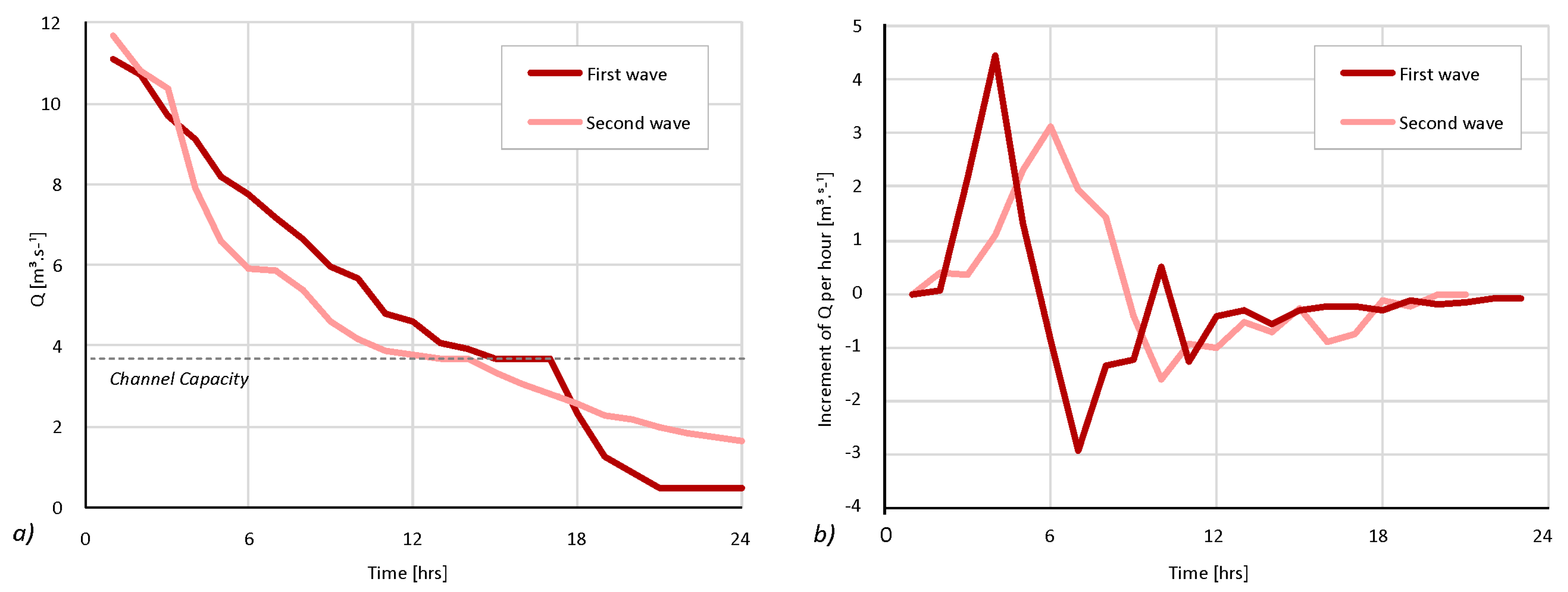
The flood event in June 2013 was the largest event recorded in the period of observation by the sensor network, with a peak discharge value of 11.7 m³·s⁻¹. The flood event consisted of two waves, both with a steep increase of the rising limb of the hydrograph with maximal rates of incrementation per hour of 3.1 and 4.4 m³·s⁻¹ for the first and second waves, respectively (Figure 10).

The peak flows in the assessed segment lasted less than 1 h. However, despite the fast progress of the peak flood wave, the channel capacity, able to transfer a discharge of 3.7 m³·s⁻¹, was exceeded in the total duration of 26 h. The threshold conditions for the full channel capacity represent the maximum flow velocity of 1.7 m·s⁻¹ and a shear stress at the most exposed site of 25 N·m⁻². Such a flow is capable of mobilizing a gravel particle of 3.5 cm in diameter or noncohesive materials of a smaller grain size. The exceedance of the channel capacity and the threshold conditions for 26 h thus had significant effects on the fluvial dynamics.

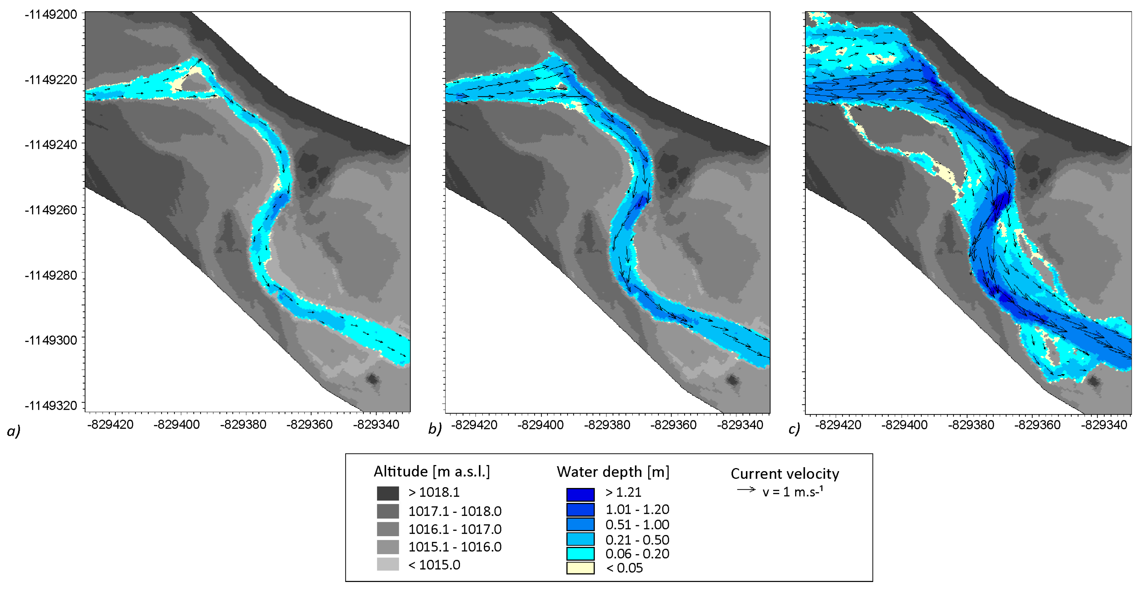
The flood wave rapidly propagated through the reach, achieving a maximal depth of 1.8 m at the concave bank, where significant erosion occurred (Figure 11). The depth-averaged velocities reached 2.1 m·s⁻¹ at the most exposed sites of the concave banks. The shear stress at the exposed sites during the flood culmination reached 67 N·m⁻², evoking significant rates of bedload and bank erosion.

3.3. Effect of Different Horizontal-Plan Schematizations

The results were evaluated for two margin situations—low flows with a discharge of 0.3 m³·s⁻¹, representing the lowest values recorded in the studied period, and high flows (11.7 m³·s⁻¹), representing the peak flow recorded for the June 2013 flood.

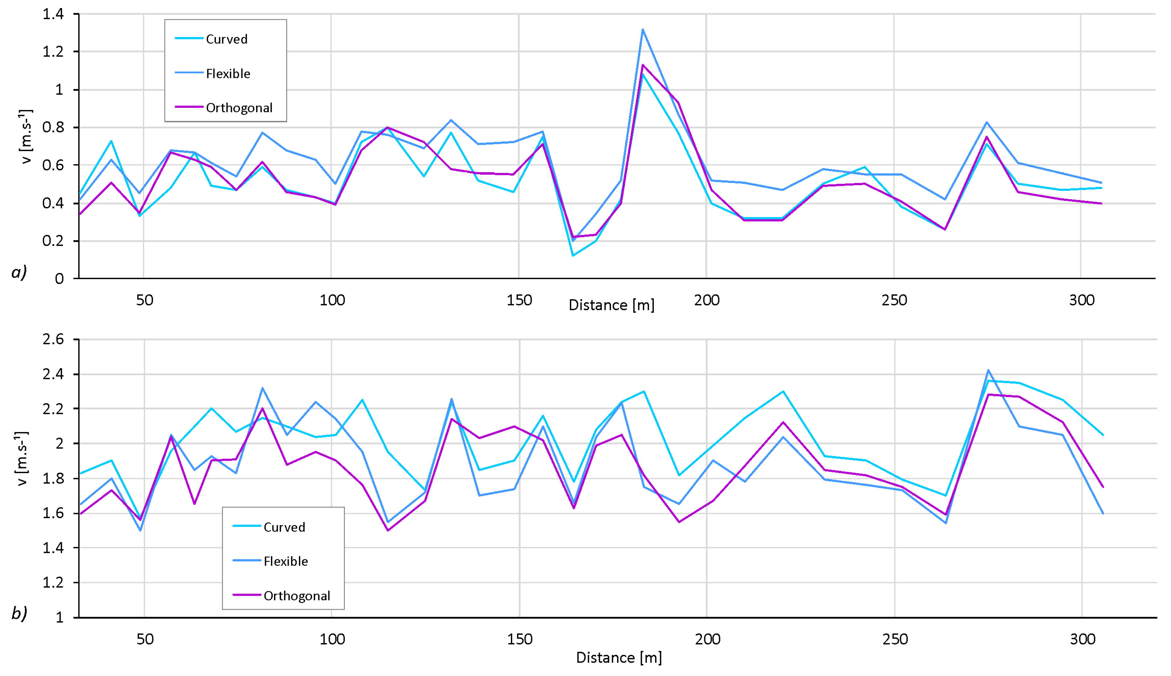
The 2D hydrodynamic model is capable of providing results in a horizontally distributed form so that the longitudinal profiles at the main flow path or cross-section at the meanders can be evaluated. The longitudinal profile of the velocity distribution was plotted for the results of the three schematization methods, namely, the orthogonal grid, curved grid and fully flexible mesh (Figure 12). The results of the point extraction are randomly selected points on a streamline; thus the effect of local extremes is reduced.

In the case of low flows, the velocity distribution computed on the flexible mesh domain (0.62 m·s⁻¹ on average, 0.20 m·s⁻¹ at a minimum and 1.32 m·s⁻¹ at a maximum) was almost constantly above the values obtained by the grid-based methods (0.52 m·s⁻¹ for both methods on average, 0.12 m·s⁻¹ and 0.22 m·s⁻¹ for curved and orthogonal at a minimum, respectively, and 1.08 m·s⁻¹ and 1.13 m·s⁻¹ for curved and orthogonal at a maximum, respectively). The variation of the velocities in low flows was 29% on average and increased with the flow depth. At high flows, the differences between the results of the three schematization methods were less significant. The variation of the velocities in high flows was 13% on average and did not show any relation to the flow depth. The average velocities were 1.89, 2.03 and 1.87 m·s⁻¹ for the flexible mesh and curved and orthogonal grids, respectively; the minimums were 1.50, 1.57, and 1.50 m·s⁻¹; and the maxima were 2.42, 2.36 and 2.28 m·s⁻¹.

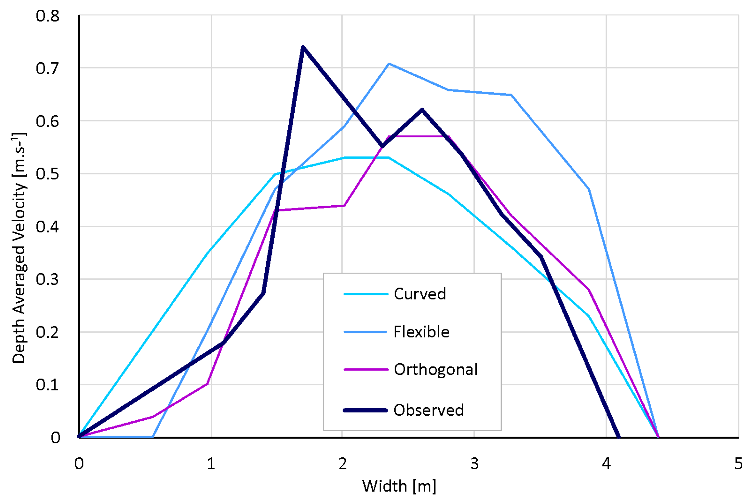
For the three types of schematizations, the cross-sectional depth-averaged velocities during the average flow (0.3 m³·s⁻¹) were compared (Figure 13) and evaluated on the basis of the observed values. The absolute values in the streamline (cross-section X = 2.5) ranged from 0.5 m·s⁻¹ in the case of the curved grid to 0.7 m·s⁻¹ in the case of a flexible mesh, representing the model domain. The stream velocity during the base flows was compared with the velocities measured under similar hydrologic conditions, producing a satisfactory fit. The differences were caused mainly by the different positions of individual domain elements varying among the schematization types.

Furthermore, the depth-averaged shear stress τ (N·m⁻²) was evaluated during the culmination at the characteristic cross-sections A (straight reach), B (left-bank failure), and C (accumulation at the right bank; Figure 14). The maximal value of the shear stress was reached at the left-bank failure—cross-section B (49, 67 and 57 N·m⁻² for the flexible mesh and orthogonal and curvilinear grids, respectively). Compared to this, lower values were obtained at the fresh accumulation reach (cross-section C), particularly at the right part, where the gravel sedimentation occurs. The straight reach (cross-section A) shows a uniform distribution of the shear stress with high values at the streamline (55, 65 and 58 N·m⁻² for the flexible mesh and orthogonal and curvilinear grids, respectively).

The comparison of different schematizations at the cross-sectional profiles indicate that the values calculated by the flexible mesh schematization were, at the most exposed sites, 20–35% lower than the results achieved using an orthogonal grid and were 15–30% lower than the values based on the curved grid. The greater the absolute value, the greater the difference. The maximal values resulted mostly from the orthogonal grid schematization with one exception, at cross-section C. Here, the shear stress calculated from the results of the curved grid schematization were 25% higher than the results of the other models. The distribution of the simulated depth was similar for all model types; thus the difference in the shear stress distribution strongly depends on the velocity distribution. The velocity at the streamline of cross-section C reached 1.8 m·s⁻¹ in the case of the curved grid and 1.65 and 1.62 m·s⁻¹ in the cases of the orthogonal grid and flexible mesh, respectively. Such a difference could indicate an accidentally steeper gradient of the channel bottom captured by the curvilinear grid model only.

4. Discussion

The spatial data derived from the UAS imagery by the photogrammetric reconstruction represent a substantial qualitative leap in the resolution and accuracy of topographic information with a high potential for the detailed simulation of dynamic processes in the riverscape [6]. The level of detail, reaching typically 1–5 cm, enables the capturing of even the finest details of the stream channel or artificial structures that are the subject of research in hydrology and fluvial geomorphology [9]. Such an ultra-high resolution of the topography can be achieved at the complex stream and floodplain segments, which allows for the development of channel models covering the processes for functional units of the riverscape.

Despite the high accuracy of the data derived from aerial LiDAR scanning [37,38] and their satisfactory resolution for general morphometric analyses, the qualitative leap in the data density in the DEM derived from the UAS is substantial (Figure 15). For the purpose of hydrodynamic modeling, the correct representation of the stream channel itself is critical. The DEM, sampled at a 2 cm resolution, enables the describing of even subtle variations of the stream channel and bank structures. Such a level of detail has no equivalent in the conventional data sources.

In addition to the ultra-fine resolution of the floodplain model, another benefit of the UAS-derived digital elevation model is the up-to-date status of the data, which can be acquired on demand to capture the true status of the landscape [39]. This aspect is of particular importance in areas undergoing changes resulting from natural processes, for example, floods or artificial modifications. While the conventional DEMs are updated with a typical period of a decade, the rapid acquisition of the terrain data by means of UASs allows for the fitting of the model to the true status of the riverscape.

However, the application of such a high-resolution elevation grid should be always considered according to the research task and application [40,41]. The use of such extremely fine resolutions is of great benefit, particularly when modeling complicated channel structures, either natural or artificial, at a high level of detail. However, the use of such detailed elevation models can be extremely demanding for the modeling in terms of the processing power and calculation time. The selection of an appropriate resolution should thus be balanced to consider the potential benefits and limitations according to the purpose of a given research task [40]. For applications in environments for which the stream and floodplain structures are not significantly complex, the initial point cloud can be rescaled to a DEM of lower resolution to decrease the computing time while retaining the accuracy to a degree that is still superior to that of conventional data sources.

Our study has also proven the limitation of UAS photogrammetry in the description of the submerged zone of the channel. Although the simulated stream is a narrow and mostly shallow montane creek, the water column depth varies significantly. The stream is unregulated, and in the meandering belt, there is a well-developed riffle-and-pool system with alternating shallow parts and deep pools with a highly turbulent flow. In a stream with an average width of 4–6 m, the water depth varies from approximately 10 cm in the shallow parts up to 1.5 m in the pools. As a result of such variability of the depth with a turbulent flow, the known experimental techniques for the estimation of the river bottom profile [8] cannot be applied. Despite the fact that the model reflects a small stream, the building of a complex 3D channel model requires auxiliary data for the reliable reconstruction of the submerged zone.

The discharge based on the automated sensor network proved to be a data source adequate to the precision of the high-resolution 3D channel model. The level of detail in terms of the sampling frequency and accuracy of the assessment enables the simulating of the elevated dynamics of runoff processes in highly dynamic montane streams. The key aspect limiting the reliable use of the data from an automatic sensor network is the proper calibration of the rating curves, which remains an element largely dependent on the design and quality of the field measurements [42]. Most of the devices applied for the automated monitoring of the runoff are based on the monitoring of the water levels and thus require the development of rating curves based on direct discharge measurements [43]. Building a reliable database is, however, a time-consuming process, particularly when covering extreme values—both on the sides of low flows and peak flows. It thus should be noted that although the technical setup of a sensor network itself is relatively rapid, the calibration of the rating curves requires time for repeated field measurements by a propeller or velocimeter.

The simulations based on different horizontal-plan schematizations exhibited different degrees of suitability with respect to the given types of the data source and channel properties. It can be seen that the general pattern of the velocity distribution in the longitudinal profile was similar for all of the schematization types, and the variation could be accounted for by the different sizes and exact positions of the domain elements or the numerical methods used (finite volume in the case of flexible mesh vs finite differences in the grid-based schematizations). Although the overall patterns of the velocity distribution during the low and high flows were comparable, the local differences of the results achieved by the different types of schematizations reached up to 30% of the depth-averaged velocity. It was observed that the lower the absolute velocity value, the greater the difference between the results obtained by the three domain representations.

During low flows, the stream velocities calculated by the flexible mesh domain remained consistently higher than those for the other schematizations. However, for peak flows, such a pattern was not observed.

The differences in the current speed calculated by the various methods can be assigned (1) to the varying geometric properties of the domains, or (2) to the different approaches of the individual numerical simulations. The first case is presented in Figure 10, showing the differences in the cross-sectional area caused by the different schematization types. The differences of the flow profile were found to range from 1.5 to 5 cm and were considered of lower importance. Furthermore, there was no correlation observed between the domain geometry and current speed differences. It implicitly follows that the differences in the current speed are rather attributed to the different numerical schemes of the three model types used. The highest differences were observed at low flows, for which the depths of the flow profile were the lowest. The flexible mesh representation derived higher current speeds at low flows. The most realistic results in comparison with the detailed measured data in low flows were obtained by the orthogonal grid representation. Nevertheless, by exploring high flows, the current speed values and patterns were similar for all the schematization types.

The distributions of the shear stress resulting from the different schematization types showed 15–35% differences at the most exposed sites between the flexible mesh schematization and the other grid-based domains. The shear stress at the stream line at the culmination reached 67 N·m⁻². Such flow conditions are capable of the mobilization of gravel particles that are 9 cm in diameter. The value of the depth-averaged shear stress is the crucial parameter for further simulation of the morphological changes. Thus, there are expected to be higher erosion rates when using the orthogonal grid-based models for transport processes.

Our study pointed to the significant effect of spatial data resolution on the reliability of hydrodynamic modeling, apparent in studies using different types of models and applications, ranging from inland rivers [33,34] to estuarine systems [44,45]. Compared to the models built from the conventional 3D data sources [17,46], the application of the ultra-high resolution data for the channel reconstruction seems to minimize the differences among the schematizations in terms of the resulting values. However, there are substantial differences in computational complexity among the schematizations, while the flexible mesh model, in particular, is substantially more demanding in terms of computational resources and time compared to the simpler schematizations of the orthogonal or curvilinear grids. For practical applications, it is suggested that the building of hydrodynamic models based on ultra-high resolution data may benefit from simpler model domain schematizations while still retaining an adequate level of reliability of the results.

5. Conclusions

Newly emerging technologies for field surveying and monitoring in the geosciences, such as UAVs (e.g., drones) and automated sensor networks, bring new types of data sources that have a high spatial accuracy, high frequency of sampling, and flexibility in designing and operating field survey campaigns, making them suitable for the detailed monitoring, analysis and modeling of risk processes, including floods.

This study demonstrated the efficiency of these data sources for the setup of a 2D hydrodynamic model with high levels of spatial and temporal detail. In addition to the unprecedented levels of detail and accuracy, the emerging monitoring techniques have a high operability that enables the reconstructing of a flood event in a remote montane creek, in an environment with a dynamic runoff response and a lack of conventional data coverage. A network of ultrasonic water level gauges with a 10 min interval was used as a source of hydrological data for the analyzed stream stretch. The MIKE 21 hydrodynamic model was used for building the flood model of the stream. The UAV platform Mikrokopter HexaXL was used for the acquisition of the aerial imagery and the further derivation of the 3D model of the terrain.

The study proved the persisting limitation of the UAV-based photogrammetric reconstruction of the stream, which, under conditions of highly turbulent flow and an irregular stream bottom, does not allow covering of the submerged zone of the channel. The 3D reconstruction of the stream was thus based on the fusion of different data sources. The UAV-based model was used for the riparian zone and stream channel, and the channel bathymetry was completed by RTK-GNSS positioning.

The application of the three types of horizontal-plan schematization applied for 2D hydrodynamic modeling—the orthogonal and curvilinear grids and the flexible mesh—indicated only marginal differences in the distribution of the flow parameters in the longitudinal profile as well as in the cross-profiles. The greatest differences between the simulated values and the observations were found under the conditions of low flows. This reflects the effect of the highly variable meandering montane stream, featuring a developed step-pool morphology and coarse bed material. The higher the water level, the lower the effect of the uncertainties related to the irregular stream channel and the closer the simulated values were to the observations. The model proved that although the peak flows of the flood were of short duration, the long-lasting high water levels exceeding the bankfull discharge for more than 26 h together with the elevated shear stress values were the decisive factors for the subsequent intense erosion at the outer banks of the meanders and for the large-scale accumulations over the point bars.

The results prove the high potential of the mutual application of UAV-based surveying and automated monitoring networks as data sources suitable for building precise and reliable hydrodynamic models. The high operability and cost efficiency of the data acquisition enables the rapid building of the model and simulations or reconstructions of risk processes in highly dynamic environments and in remote areas with a lack of conventional data coverage.